WaterProof—A Web-Based System to Provide Rapid ROI Calculation and Early Indication of a Preferred Portfolio of Nature-Based Solutions in Watersheds

Abstract

Watersheds are being degraded around the world, with dire impacts on water security. Nature-based solutions (NbS) can preserve or restore degraded watersheds, thereby addressing critical water security issues; however, there is a lack of NbS uptake and investment. This is in part due to the complexity and time required to demonstrate an NbS portfolio’s positive return on investment (ROI) for desired water security outcomes. WaterProof is a web-based decision support tool to provide a rapid ROI calculation and early indication of a preferred portfolio of NbS for any watershed in the world using Natural Capital ecosystem service models (InVEST and RiOS). WaterProof is intended to engage stakeholders interested in exploring green infrastructure solutions for local water challenges and for prioritization of locations of possible NbS water security programs. WaterProof version 1.0 is freely available and open-sourced, with clear methodology and metadata, with a user-friendly interface suitable for a wide range of potential audiences.

1. Introduction

Accelerated degradation of the world’s watersheds has reached levels where the water crisis may limit food production, ecosystem functions and urban water supply [1,2,3,4]. Nature-based solutions (NbS) have the potential to conserve and restore watersheds [5,6,7,8]. However, a fundamental step of NbS investments is to assess the return on investment (ROI) of NbS and to ensure a clear and transparent process in this assessment to better inform decision making [9]. These analyses can be greatly facilitated by the use of tools to analyze and economically value the water security benefits of NbS to ensure a positive return on proposed investments.

From the perspective of a watershed investment program [10], in the pre-feasibility phase, it is very important to be able to assess the potential for NbS to address water security challenges, but the effort required to analyze the ROI in this phase is often time- and cost-prohibitive [11]. Considering this need, we have developed WaterProof as a free web-based tool for high-level ROI assessment, designed to provide stakeholders interested in NbS with a pre-feasibility assessment regarding NbS potential.

Currently, there are different web tools that allow the identification of NbS portfolios, as well as the estimation of their social, hydrological, ecological and environmental co-benefits. For example, Ref. [12] proposed a general framework and a web tool for pre-selection of NbS projects that interrelate governance, financing and business models. The authors in [13] developed the Landslide Risk Mitigation Toolbox (LaRiMiT), a web-based tool to identify and select mitigation measures for mass movements from an extensive database of structural solutions and NbS. The authors in [14] designed a National Spatial Data Infrastructure web system to identify NbS benefits in the United States. The authors in [15] generated an interactive web-based application that enables green infrastructure planning in different urban contexts and [16] built a generalizable web application to engage stakeholders in the spatial planning of ecosystem restoration and NbS using spatial prioritization of green roof retrofitting in Oslo, Norway.

While all the above tools represent a great contribution to the understanding of NbS, none of them focuses on ROI analysis for the operation and maintenance of drinking water supply system infrastructure (including drinking water treatment plants—DWTP). WaterProof version 1.0 aims to contribute to bridge this gap. This version uses global databases for modeling and analysis. In this first version, we used the Resource Investment Optimization System (RiOS) [17] for analysis and generation of NbS portfolios and Integrated Valuation of Ecosystem Services and Tradeoffs (InVEST) [18] for ecosystem services modeling. We also incorporated algorithms in WaterProof for financial analysis and economic valuation of benefits for ROI calculation [11,19,20].

The technological solution implemented uses cloud computing for the execution of mathematical models and analysis tools, using Amazon Web Services (AWS). WaterProof is a technological innovation with the objective of carrying out ROI analysis, at pre-feasibility level, in a few minutes, as compared with several months with a more traditional approach.

2. System Design

The process followed for the development of WaterProof is divided into two main stages: (1) Design and (2) Implementation. The objective of the design stage was to clearly define the functionalities of the system. We used an enterprise architecture approach to develop the design of the tool and, in parallel, we conceptualized its calculation structure and analysis flow, defined modeling and analysis tools and identified global databases and data structure. The design was user-oriented, so we initially carried out a work process with stakeholders to define a general concept of the tool and capture the needs and expectations of the potential users. With this foundation, we were able to carry out the technical development of the design for the definition of the functional requirements of the platform.

In the implementation stage, we defined the software architecture and developed the code of the web application having as a guide the functional requirements identified during the design, but under an agile software development methodology [21] that allowed us to be flexible to incorporate specific needs during the development.

The following is a summary of the most relevant elements used in the design of the system.

2.1. Enterprise Architecture Approach

According to [22], Enterprise Architecture can be defined as “a coherent set of principles, methods, and models that are used in the design and implementation of organizational structure, business processes, information systems, and information infrastructure of a company”. Having a vision in the development of Information Technology (IT) that is adequately articulated for the solution of business problems is fundamental in the design of tools that respond to the needs of users and adequately support the business [23].

The process of creating a useful technological solution that involves the analysis of water systems and watersheds is especially challenging given the complexity involved in understanding hydrological processes and the complex relationships that stakeholders in a watershed need to know for decision making [24]. Additionally, if elements associated with the conservation of aquatic ecosystems, NbS and financial elements for investment analysis are incorporated, the challenge is even greater, so that a technological solution of this type requires for its design a technical framework in which the principles, methods and models are integrated.

In this regard, we used an Enterprise Architecture approach to facilitate the conceptualization and design of the software solution. As part of the design process, we focused our analysis on 5 main components: user definition and characterization, identification of principles, themes and fundamentals, data sources and objective software architecture.

Through workshops developed with different stakeholders, we defined a first draft of the desired capabilities of the system as well as some conceptual elements of results reporting that were consolidated into a prototype of the application. This first exercise was fundamental to understand that the system should support three different types of users: administrator, general public and analyst. Consistent with a process in which users are considered at the center of software solution development, we define these three types of users for WaterProof as follows:

• Administrator: User in charge of managing the website, granting permissions to users, managing information, guaranteeing platform security and performing system updates.
• General public: Users interested in knowing about nature-based solutions in watersheds, consulting analysis cases and seeing results of cases previously executed and created by other users. This user does not create or develop case studies and does not use the capabilities of the system in cloud computing.
• Analyst: An advanced user of the system interested in configuring their own case studies, with access to cloud computing capabilities to run, analyze, share and compare case studies.

We established 17 main functionalities of the system for the three types of WaterProof users. Figure 1 summarizes this information.

In order to have fluid communication with the software development team, we developed a document of themes and fundamentals in which we included the concepts that support the development of the IT solution. This was a document that facilitated communication between the hydrology and finance technicians and the software development engineers. The document included basic definitions of watershed and hydrology, ecosystem services, nature-based solutions, mathematical modeling, infrastructure for water supply systems and return on investment analysis.

To identify the data sources for the system, we conducted an extensive review of the global databases available for each of the variables required for the analyses and modeling, so that we could identify the most appropriate databases for the system. Details of the databases included within the system are provided later.

Finally, we defined the software architecture of the IT solution. This process included defining 38 fully documented functional requirements for the software developers in conjunction with an extensive use case document.

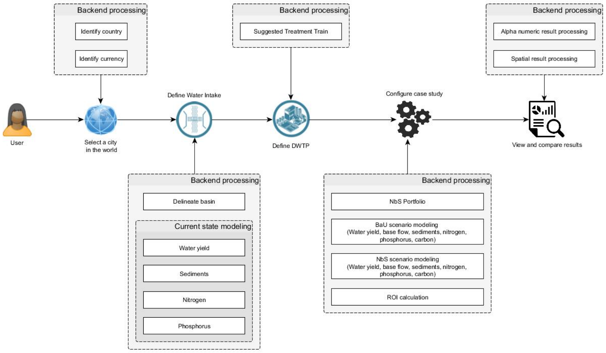
2.2. Conceptualization of the System and Analysis Flow

We performed a conceptualization of the system focused on defining a clear analysis flow to identify user interactions with the system as well as the processing and modeling needs from the backend. The conceptualization of the analysis flow is presented in Figure 2.

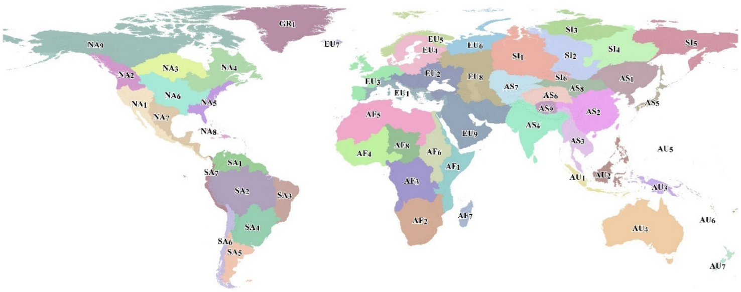
In this design, an analyst user in WaterProof starts by selecting a city in the world for which their analysis will be associated. We use the city as a way to organize information within the system and also to identify the currency of the country to which the city belongs. As part of the design, it was defined that although the currency of the country is a guide for the system, users are free to define the costs in any currency they wish, and WaterProof will be able to perform currency transformations based on exchange rates.

Once the user has identified the city, the next step is to define and characterize the water intake. For this process, we established four main steps:

• Define location of water intake: The user must indicate the name of the water intake, a brief description, the name of the water source and indicate on a map the point of the water intake either by clicking on the map or by entering the coordinates. Using the water intake point as closure point, WaterProof processes the digital elevation model (DEM) to delineate the catchment. This is performed using conventional DEM processing for watershed identification [25].
• Define water intake infrastructure: With a drag-and-drop scheme, the user can indicate the infrastructure elements that are part of the water intake and connect them. For each element, the user can edit the percentage of water transported, percentage of sediment retained, percentage of nitrogen retained and percentage of phosphorus retained. Additionally, each infrastructure element can have associated cost functions. Cost functions are mathematical expressions that allow the establishment of operation and maintenance costs for each infrastructure element based on variables calculated by the system. WaterProof interprets this information as a topologically connected system on which it is possible to perform water, sediment, nitrogen and phosphorus balance calculations using transport and retention rates.
• For WaterProof version 1.0, a user can use 10 infrastructure elements to represent water intake: (1) Reservoir, (2) Pumping, (3) Raw water reservoir, (4) Bottom intake, (5) Side intake, (6) Floating intake, (7) Desander, (8) Brake pressure chamber, (9) External input and (10) Drinking water treatment plant. Note that WaterProof can consider inter-basin transfers with the external input element; using this element, users can directly enter flow rate series and sediment, nitrogen and phosphorus series.
• Define water demand: The user must indicate the water demand (water withdrawal from the source). This is defined as a time series. WaterProof offers two main ways to generate the input data: Using interpolation methods where the user indicates the demand in the initial and final years and selects the preferred interpolation method among 4 available methods: (i) linear interpolation, (ii) potential interpolation, (iii) exponential interpolation or (iv) logistic interpolation. The second way to enter demand information is directly by entering the time series year by year in a data table.
• Define NbS implementation area: The user can define the area within the watershed in which NbS will be developed. By default, the system will consider that NbS can be developed in the entire watershed area, however, a user can define specific areas where NbS implementation is restricted. WaterProof allows defining these areas by drawing them directly on the map or by uploading an SHP file with the polygons that delimit the areas where NbS implementation is possible.

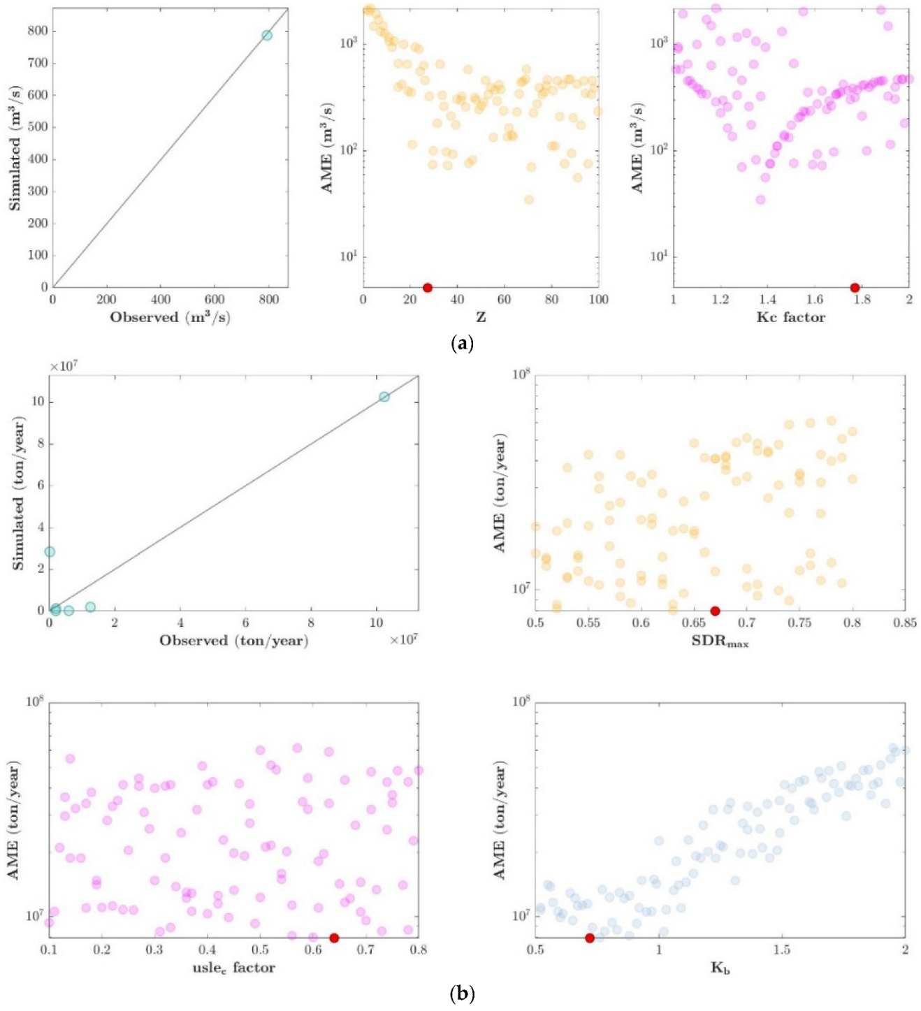
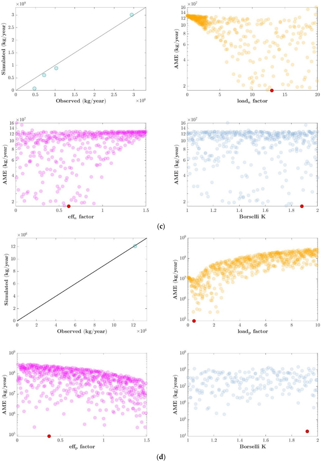
At the end of the water intake configuration, WaterProof performs a first analysis with the objective of estimating the current water quality conditions at the water intake point. For this, a first simulation is performed using four models from the InVEST package [18]: Annual Water Yield, Sediment Delivery Ratio, Nutrient Delivery Ratio (Nitrogen) and Nutrient Delivery Ratio (Phosphorus). WaterProof uses the current land use/land cover condition for this simulation. With this information, WaterProof estimates the concentrations of sediment, nitrogen and phosphorus in the water body at the water intake point.

The next step is for the user to define the processes that are part of the drinking water treatment plant under analysis. In this section, WaterProof uses the information on sediment, nitrogen and phosphorus concentrations obtained earlier as an estimate of the water quality characteristics at the water source, and additionally uses information from a database that indicates by country the regulatory requirement for drinking water treatment to suggest a pre-selected treatment train to the user. The authors in [26] carried out an extensive literature review to define a database that classify the levels of requirement for drinking water treatment for each country using the criteria shown in

Table 1. Criteria for classification of regulatory requirements for the treatment of drinking water by country (Csed: Concentration of total suspended solids, CN: Concentration of nitrogen).

Category	1	2	3	4
Criteria 1	Csed ≤ 2.65 mg/L	2.65 mg/L < Csed ≤ 5.6 mg/L	5.6 mg/L < Csed ≤ 17 mg/L	Csed > 17 mg/L
Criteria 2	CN ≤ 5 mg/L	5 mg/L < CN ≤ 11 mg/L	11 mg/L < CN ≤ 20 mg/L	CN > 20 mg/L

. As part of the Supplementary Material, the database with the classification adopted in WaterProof for each country can be consulted.

Criteria were also defined to categorize water quality at the source according to the analyses presented by [26]. Using the results of the first modeling in the current condition, WaterProof classifies the water quality at the source using the criteria in

Table 2. Criteria for classification of water quality in the source (Csed: Concentration of total suspended solids, CN: Concentration of nitrogen, CP: Concentration of phosphorus).

Category	A	B	C	D
Criteria 1	Csed ≤ 4.4 mg/L	4.4 mg/L < Csed ≤ 56 mg/L	56 mg/L < Csed ≤ 203 mg/L	Csed > 203 mg/L
Criteria 2	CN ≤ 10 mg/L	10 mg/L < CN ≤ 20 mg/L	20 mg/L < CN ≤ 30 mg/L	CN > 30 mg/L
Criteria 3	CP ≤ 0.2 mg/L	0.2 mg/L < CP ≤ 1 mg/L	1 mg/L < CP ≤ 4 mg/L	CP > 4 mg/L

.

WaterProof suggests to the user an expected treatment train for the drinking water treatment plant (DWTP) based on seven typified DWTPs according to the water quality category required by regulations in the country and the water quality category at the source [26].

Table 3. Active treatment train processes for each type of DWTP.

DWTP Type	A	B	C	D	E	F	G
Dosage	X	X	X	X	X
Quick mixing	X	X	X	X	X
Slow mixing	X	X	X	X	X
Sedimentation	X	X	X	X	X
Filtration	X	X	X	X	X	X	X
membrane filtration (Retained particle size 0.1 µm)	X	X			X
membrane filtration (Retained particle size 0.0001 µm)	X
Ion Exchange		X	X
Disinfection	X	X	X	X	X	X
Sludge treatment	X	X	X	X	X	X

shows the active processes in the treatment train for each of the typified DWTPs and

Table 4. Scheme used by WaterProof for the definition of the typical DWTP suggested by the system considering the analysis presented by [26].

	Category of Regulatory Requirements for the Treatment of Drinking Water
Category of Water Quality in the Source	1	2	3	4
A	DWTP E	DWTP F	DWTP G	DWTP G
B	DWTP E	DWTP D	DWTP F	DWTP F
C	DWTP B	DWTP C	DWTP D	DWTP D
D	DWTP A	DWTP A	DWTP C	DWTP D

shows the scheme used by WaterProof for the definition of the typical DWTP.

The system shows the expected active processes of the DWTP according to the typification performed; however, the user can modify the processes considered by enabling or disabling the corresponding processes for the analysis. Additionally, the user can select or create technologies associated with each of the treatment processes. We included some technologies as part of the system that are typically used in the different processes of the treatment train that the user can select according to the specific conditions of the DWTP, which are summarized in

Table 5. Technologies available by default for selection in WaterProof in each process of the treatment train.

Process	Technology
Dosage	Liquid aluminum sulfate
	Granulated aluminum sulfate
	Ferric chloride
	Polymer
Quick mixing	Hydraulic mixing
	Mechanical mixing
Slow mixing	Hydraulic flocculation
	Mechanical flocculation
Sedimentation	Conventional settler
	High-rate settler
	Sludge blanket decanter
Filtration	Rapid mixed-bed filtration
	Rapid single-bed filtration
	Single-bed slow filtration
Membrane filtration (retained particle size 0.1 µm)	Microfiltration
Membrane filtration (retained particle size 0.01 µm)	Ultrafiltration
Membrane filtration (retained particle size 0.001 µm)	Nanofiltration
Membrane filtration (retained particle size 0.0001 µm)	Inverse osmosis
Ion Exchange	Ion Exchange
Disinfection	Chlorine gas
	Chlorine in situ
Sludge treatment	Sludge pumping
	Sludge thickener
	Drying beds
	Filter press

, without this meaning that the system is limited to this list, considering that a user can flexibly define the technologies for the analysis.

Users can select the technologies that best represent the conditions of their analysis infrastructure but can also add new technologies with specific cost functions to be considered as part of the analysis under a fully customized scheme.

With the definition of the water intake and the DWTP, the user can set up the case study. A case study is the way WaterProof analyzes the operation and maintenance costs of the infrastructure, including the possible benefits of NbS. For the configuration of a case study, the system assists users through seven steps:

• Define infrastructure for analysis: In this step, users must indicate the name of the case study for its identification and the water intakes and DWTPs they want to include as part of the ROI analysis. WaterProof allows multiple water intakes and DWTPs to be included in a single case study.
• Carbon market benefit: WaterProof can consider the economic benefit associated with the carbon market. For this, the user must activate the option and indicate the benefit in money per ton of CO2eq. WaterProof suggests to the user a carbon market benefit value taken from [27], but the user can edit this value according to their local condition.
• Define portfolio objectives: The user must indicate the objectives for which the NbS portfolios will be constructed. WaterProof version 1.0 uses RiOS (Resource Investment Optimization System) [17] as the software for the construction of the NbS portfolios. In this regard, the user can select the objectives for the portfolio from seven options available in RiOS: (1) Erosion control for drinking water quality, (2) Erosion control for reservoir maintenance, (3) Nutrient retention (phosphorus), (4) Nutrient retention (nitrogen), (5) Flood mitigation, (6) Groundwater recharge enhancement and (7) Baseflow.
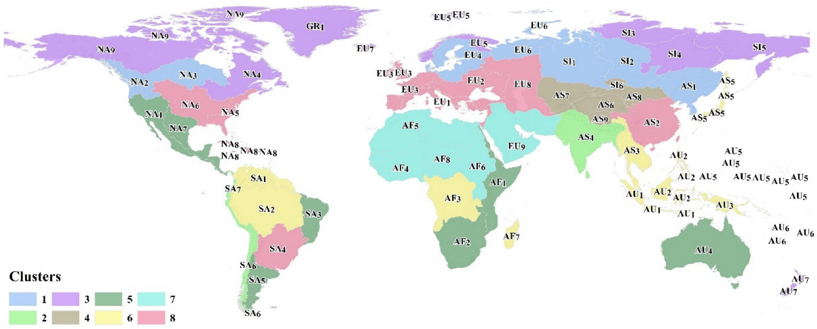
• Define InVEST modeling parameters: WaterProof performs mathematical modeling using the InVEST models [18]: (1) Annual Water Yield (AWY), (2) Seasonal Water Yield (SWY), (3) Sediment Delivery Ratio (SDR), (4) Nutrient Delivery Ratio—Phosphorus (NDR—P), (5) Nutrient Delivery Ratio—Nitrogen (NDR—N) and (6) Carbon Storage and Sequestration (CSS). The system loads by default the pre-defined biophysical parameters for these models according to the location in the world where the analysis is performed. However, users can edit the modeling biophysical parameters if they have specialized information. WaterProof allows editing the values of 40 biophysical parameters associated with the six mathematical models. Detailed information on these parameters can be found in the InVEST documentation [18]. This option was proposed for advanced users.
• Define financial parameters: In this step, users can define financial parameters for the analysis and include the operating costs of the program in charge of the NbS implementation. Within the annual costs of the program, users can indicate personnel salary and benefits, office costs, travel expenses, equipment, vehicles and overhead and transaction costs. WaterProof suggests the value of these costs according to the experience in different countries of The Nature Conservancy (TNC) knowledge conservation programs; however, all values can be edited by the users. Finally, the discount rate for the ROI analysis must be indicated. In this case, the system allows the user to enter a discount rate for the analysis and a minimum and maximum discount rate in order to perform a simple sensitivity analysis. The system suggests the discount rate values, taking as reference [28]; however, users can modify the values according to their more detailed information.
• Define NbS for analysis: Users must select the NbS they wish to consider for the case study analysis. By default, five NbS are configured in the system available to all users for selection: (1) Forest conservation, (2) Active restoration—Enrichment, (3) Passive restoration, (4) Agroforestry and (5) Silvopastoral systems. These NbS were created in the system as examples only, however, WaterProof allows a user to create their own NbS. During this NbS creation process, the user must parameterize the NbS by indicating its name, time required to obtain maximum benefits, benefit percentage at time t = 0, maintenance periodicity, implementation cost, maintenance cost, opportunity cost and land use/land cover transition.
• It is important to note that the definition of the NbS is limited to the conceptualization of RiOS as an analysis software, so in version 1.0 of WaterProof, it is only possible to represent an NbS that fits the seven categories of land use transitions available in RiOS [17]: (1) Keep native vegetation, (2) Revegetation (unassisted), (3) Revegetation (assisted), (4) Agricultural vegetation management, (5) Ditching, (6) Fertilizer management and (7) Pasture management.
• Define analysis parameters: As a final step, users must define the analysis parameters corresponding to: analysis time period, implementation NbS period and yearly budget and climate for analysis. WaterProof can perform the analyses considering historical climate or under six climate change scenarios associated with the following global circulation models: (1) RCP4.5 BCC-CSM2-MR, (2) RCP4.5 CNRM-ESM2-1, (3) RCP 4.5 MIROC6, (4) RCP8.5 BCC-CSM2-MR, (5) RCP8.5 CNRM-ESM2-1 and (6) RCP 8.5 MIROC6.

Once the case study configuration is completed, WaterProof will start the calculation sequence, which has four main steps:

• Calculation Step 1—NbS Portfolio: Considering the NbS selected for analysis, the objectives defined for the portfolio and the investment budget, WaterProof runs RiOS [17] to define the NbS investment portfolio. As a result of this calculation step, the year-by-year investment portfolio is obtained in raster format together with the total NbS implementation areas and the implementation and maintenance costs. Additionally, WaterProof has an algorithm that allows generating a raster of land uses considering the effect of change in coverage expected by the implementation of the NbS. The expected future land use/land cover raster incorporating the effect of NbS is defined in the system as the layer in the NbS scenario.
• Calculation Step 2—Business as Usual (BaU) scenario modeling: WaterProof performs the simulation of ecosystem services for a BaU land use/land cover scenario using the InVEST models: (1) Annual Water Yield (AWY), (2) Seassonal Water Yield (SWY), (3) Sediment Delivery Ratio (SDR), (4) Nutrient Delivery Ratio—Phosporus (NDR-P), (5) Nutrient Delivery Ratio—Nitrogen (NDR—N) and (6) Carbon Storage and Sequestration (CSS). WaterProof has layers in raster format incorporated in its database that represent the expected changes in land use/land cover in BaU scenarios year by year until the year 2100, using as a basis the results obtained by [29]. In this sense, when the user performs an analysis with a specific time horizon, WaterProof identifies the land use/land cover layer directly associated with the time period of analysis according to the prospective land use change and uses this layer to perform the simulation of ecosystem services.
• Calculation Step 3—Nature based Solutions (NbS) scenario modeling: WaterProof performs the simulation of ecosystem services for a NbS land use/land cover scenario using the InVEST models: (1) Annual Water Yield (AWY), (2) Seassonal Water Yield (SWY), (3) Sediment Delivery Ratio (SDR), (4) Nutrient Delivery Ratio—Phosporus (NDR-P), (5) Nutrient Delivery Ratio—Nitrogen (NDR—N) and (6) Carbon Storage and Sequestration (CSS). For this simulation, WaterProof uses the expected land use layer associated with the implementation of the NbS. For this, it uses the result obtained in the Step 1 calculation.
• Calculation Step 4—ROI calculation: Finally, with the simulation results of ecosystem services for the BaU and NbS scenarios, financial calculations are made to estimate the return on investment. As a first procedure, it is necessary to approximate the changes in ecosystem services over time. Since the InVEST models implemented in WaterProof are long-term response models without a modeling time step, WaterProof assumes that the change in ecosystem services follows the distribution of a logistic function:

  $$w=\frac{w_{max}}{1+\left(\left(w_{max}/w_0\right)-1\right)\exp \left(-rt\right)}$$

  (1)

  where:
  $w$ = The expected change in the ecosystem service at time t;
  $w_{max}$ = Maximum change in the ecosystem service estimated by InVEST simulation;
  $w_0$ = Ecosystem service estimated at time $t$ = 0;
  $r$ = Logistic function parameter calculated for $w$ = $w_{max}$ at $t$ = $t_{max}$;
  $t$ = Time.
• Using the expected response of change in ecosystem services distributed over time with the logistic function, WaterProof calculates the operation and maintenance costs for each of the infrastructure elements in the water intake and the DWTP to which cost functions are associated. The calculation is performed for the BaU and NbS scenarios. The difference between the costs of the two scenarios is defined as the benefit. Note that the analysis is performed under the principle of comparison of two possible futures: BaU future and NbS future. WaterProof also calculates investment costs over the entire analysis period considering implementation, maintenance and opportunity costs associated with the NbS, as well as costs associated with the conservation program (personnel salary and benefits, office costs, travel expenses, equipment, vehicles and overhead and transaction costs). WaterProof calculates total and discounted costs and benefits using the discount rates defined for the case study. The ROI is calculated as the monetary benefit divided by the costs. An ROI exceeding 1 indicates a positive return on investment, while an ROI less than 1 indicates a negative return on investment [11].

Finally, we incorporated several tools in the system for processing the results obtained and facilitating their visualization. The results include a general summary in which the value of ROI obtained and net present values are presented in the main categories of implementation, maintenance, opportunity, transaction, platform (conservation program), benefit and total. A synthesis of risks in the basin is performed using information from Aqueduct [30] in the categories of water quantity risk, water quality risk, regulatory and reputational risk and overall water risk score. The NbS investment is summarized with the implementation areas for each NbS and its associated total cost. The estimate of the maximum change in each of the ecosystem services is associated with annual water yield, base flow, sediment delivery ratio, nutrient delivery ratio—phosphorus/nitrogen delivery ratio—and carbon storage and sequestration. This change in ecosystem services is calculated as a relative difference between the BaU and NbS scenarios with the equation:

$$C_{ES}=\frac{E{S}_{NbS}-E{S}_{BaU} }{E{S}_{BaU}}$$

(2)

where:

$C_{ES}$ = Change in ecosystem service;

$E{S}_{NbS}$ = Ecosystem service valued in the NbS scenario;

$E{S}_{BaU}$ = Ecosystem service valued in the BaU scenario.

Additionally, WaterProof allows exploring detailed results associated with financial indicators, physical indicators, decision indicators and geographic visualizations. The information contained in each of these detailed results sections is briefly presented below:

• Financial indicators: Users can review the detailed results for each of the benefit and cost components of the case study analysis; they can review the net present values and the result of the sensitivity analysis on total discounted benefits and total discounted costs using the discount rate’s minimum, nominal and maximum indicated for the analysis.
• Physical indicators: Users can consult the results of expected changes in ecosystem services over time in the analysis period; they can consult all indicators available in Aqueduct [30] for the basin of analysis, including the current status and projected future situations in 10 and 20 years. Users also have access to the detail of the amount of area of implementation of each NbS and the expected change in ecosystem services distributed over time (year to year) with the logistic function.
• Decision indicators: Users can view detailed costs and benefits for each of the infrastructure elements of analysis, as well as review the efficiency of the NbS portfolio in relation to each ecosystem service and a synthesis of the opportunity for investment in nature-based solutions based on return-on-investment results.
• Geographic visualization: WaterProof provides users with spatial visualizations for the comparison of current and expected land use coverages in the BaU and NbS scenarios. It also allows visualization of InVEST modeling results in raster format and spatial visualization of the NbS portfolio.

Finally, WaterProof allows users to download a PDF that synthesizes the results obtained, and additionally, it is possible to download a compressed ZIP file containing all modeling and analysis results in raster, SHP and Excel formats, so that a user can review in detail the entire calculation process in a clear and transparent manner.

2.3. Modeling and Analysis Tools

WaterProof uses Resource Investment Optimization System (RiOS) [17] for the construction of NbS portfolios and Integrated Valuation of Ecosystem Services and Tradeoffs (InVEST) [18] for ecosystem services modeling of Annual Water Yield (AWY), Seassonal Water Yield (SWY), Sediment Delivery Ratio (SDR), Nutrient Delivery Ratio—Phosporus (NDR-P), Nutrient Delivery Ratio—Nitrogen (NDR—N) and Carbon Storage and Sequestration (CSS). Both software were developed by Natural Capital Project in the Python programming language. In consideration of this, the financial analysis tools and additional processing tools were also developed in Python.

Table 6. Main modeling and analysis tools used in WaterProof.

Tool	Purpose in WaterProof
RiOS	Defines the NbS portfolio
Reclassify.py	Translates the activities defined in the portfolio to LULC expected in the NbS scenario.
InVEST	Models AWY, SWY, SDR, NDR-N, NDR-P and CSS ecosystem services in the current, BaU and NbS scenarios.
Select_PTAP.py	Defines, according to the water quality conditions in the water intake and the country’s regulations, the expected active processes in the DWTP treatment train.
WI_Balance.py	Calculate water, sediment, nitrogen and phosphorus balances in the water intake and DWTP infrastructure according to retention rates.
Disaggregation.py	Calculates ecosystem services disaggregated over time under the assumption of a logistic function distribution.
ROI.py	Performs all necessary calculations of monetized costs and benefits to estimate the ROI in the case study.
Indicators.py	Calculation of the indicators of change in ecosystem services, which are available for consultation in the results section.

summarizes the main modeling and analysis tools.

As part of the modeling process with InVEST, for the Annual Water Yield (AWY), Seasonal Water Yield (SWY), Sediment Delivery Ratio (SDR) and Nutrient Delivery Ratio—Nitrogen (NDR) models, a parametric consistency analysis was performed using Monte Carlo simulations. It is important to note that this process is limited by the global scale implicit in WaterProof and is therefore considered only as a guide for users on the performance of the models. The following is a description of the parametrization of the models and the parametric consistency analysis performed.

2.3.1. Parameters of the AWY Model

The parameters of the Annual Water Yield (AWY) model are presented in

Table 7. Annual Water Yield model parameters.

Parameter	Symbol	Unit	Range
Evapotranspiration coefficient	Kc	Dimensionless	[0; 1.2]
Parameter Z	Z	Dimensionless	[1; 100]

. For consistency analysis purposes, the Z parameter was varied in a range from 1 to 100. The Kc parameter was initially estimated through the mathematical expression recommended in the InVEST user’s guide, which involves the leaf area index (LAI). The LAI that was considered corresponded to MODIS products [31]. Since, for the model, a Kc must be defined for each LULC, a multiplying factor between 1 and 2 was applied to this parameter to vary proportionally the values of each LULC. As an evaluation rule, if the factor generated a Kc greater than 1.2, it was set at that value.

2.3.2. Parameters of the SWY Model

The parameters of the Seasonal Water Yield model are presented in

Table 8. Seasonal Water Yield model parameters.

Parameter	Symbol	Unit	Range
Curve Number	CN	Dimensionless	Fixed
Evapotranspiration coefficient	Kc	Dimensionless	[0; 1.2]
Parameter 1	Alpha_m	Dimensionless	[0; 1]
Parameter 2	Beta_i	Dimensionless	Fixed
Parameter 3	gamma	Dimensionless	[0; 1]

. In this model, the parameters that were analyzed for the parametric consistency analysis were Alpha_m and gamma, since; the curve numbers (CN) were obtained from the study developed by [31]. Monthly Kc was estimated using LAI according to the established method in the user’s guide of the AWY model. It is important to mention that the multiplier factor for each LUCL obtained for the AWY model was also applied to the monthly Kc. Finally, the beta_i parameter was set to a fixed value of 1, according to the recommendation of the user’s guide of the model [18].

2.3.3. Parameters of the SDR Model

The parameters of the Sediment Delivery Ratio model are presented in

Table 9. Sediment Delivery Ratio model parameters.

Parameter	Symbol	Unit	Range
Cover-management factor	usle_c	Dimensionless	[0; 1]
Support-practice factor	usle_p	Dimensionless	Fixed
Parameter 1	Kb	Dimensionless	[0.5; 2]
Parameter 2	ICo	Dimensionless	Fixed
Borselli SDRmax Parameter	SDRmax	Dimensionless	[0.5; 0.8]

. For the coherence analysis, the parameters usle_c, Kb and SDR_max were evaluated. The usle_c parameter was evaluated through a proportional multiplied factor for each LULC. The usle_p parameter was set to 1 for all land cover and land use, according to the recommendation given by [32]. Finally, the ICo parameter was set to a value of 0.5 according to the recommendation of the user’s guide [18].

2.3.4. Parameters of the NDR Model

The Nutrient Delivery Ratio model parameters are presented in

Table 10. Nutrient Delivery Ratio model parameters.

Parameter	Symbol	Unit	Range
Maximum retention efficiency—Phosphorus	eff_p	Dimensionless	[0; 1]
Maximum retention efficiency—Nitrogen	eff_n	Dimensionless	[0; 1]
Retention length—Phosphorus	crit_len_p	m	Fixed
Retention length—Nitrogen	crit_len_n	m	Fixed
Dissolved nutrient ratio	ratio_suface_n	Dimensionless	Fixed
Borselli parameter k	k	Dimensionless	[1; 2]
Subsurface critical length—Phosphorus	LCS_p	m	Fixed
Subsurface critical length—Nitrogen	LCS_n	m	Fixed
Maximum subsurface retention efficiency—Phosphorus	EMR_p	Dimensionless	Fixed
Maximum subsurface retention efficiency—Nitrogen	EMR_n	Dimensionless	Fixed
Load exported factor—Phosphorus	F_load_p	Dimensionless	[1; 20]
Load exported factor—Nitrogen	F_load_n	Dimensionless	[1; 20]

. For this model, the LCS_p and LCS_n parameters were set to a value of 200 m, while the EMR_p and EMR_n parameters were set to a value of 0, all in accordance with the recommendations of the user’s guide of the model [18]. The retention distances for both phosphorus and nitrogen (crit_len_p, crit_len_n) were set to a value of 200 m, a value which is less than the pixel resolution and is consistent with the recommendation in the user guide [18]. Finally, the ratio_surface_n parameter was set to a value of 0, in order not to consider subsurface aspects in the modeling.

The efficiencies for both phosphorus and nitrogen (eff_p, ff_n) were affected by a multiplying factor ranging from 0 to 1.5, maintaining proportionality between land cover and land use. The base values for these parameters were established according to [18]. The parameter k was varied between 1 and 2. Finally, a multiplying factor ranging from 1 to 20 was also applied to the loads exported for each LULC considering that according to the literature, loads exported have a wide variation.

2.3.5. Parameters of the CSS Model

The parameters of the Carbon Storage and Sequestration model are presented in

Table 11. Carbon Storage and Sequestration model parameters.

Parameter	Symbol	Unit	Range
Carbon density of aboveground biomass	c_above	t/ha	Fixed
Carbon density of belowground biomass	c_below	t/ha	Fixed
Carbon density of soil	c_soil	t/ha	Fixed
Carbon density of dead matter	c_dead	t/ha	Fixed

. All parameters were obtained from the literature [33,34].

2.3.6. Parametric Consistency Analysis

For the parameters identified with possible ranges of variation, a simple analysis was performed to select the parameters that were most consistent with available observations. For this analysis, we used the flow, sediment, phosphorus and nitrogen data consolidated in the GEMS-GLORI database [35]. The data to validate the SWY model were the mean actual evapotranspiration; these rasters were collected as part of the inputs for the models and are explained in more detail in the section on WaterProof’s global databases.

A total of 923 monitoring points around the world were found in the GEMS-GLORI database [35]. However, not all of them had all the information for model verification. In total, 244 points were filtered for flow, 205 points for suspended sediment concentration, 111 for nitrogen concentration and 26 for phosphorus concentrations.

For a practical working purpose for the analysis, Hydrosheds level 2 [36] was used in WaterProof for the identification of global macro-areas, as presented in Figure 3.

In total, 56 macro-areas of Hydrosheds level 2 were identified on the planet.

Table 12. Number of macro-areas with data available for the parametric consistency analysis.

Model	Number of Macro-Areas with Available Data
AWY	44
SWY	56
SDR	41
NDR-N	39
NDR-P	12

shows the number of macro-areas with data available for the parametric consistency analysis exercise. Since actual evapotranspiration information is used for the SWY model, information is available for all macro-areas.

For parameter sampling in the parametric consistency analysis of AWY, SDR and NDR models, we used the Latin Hypercube Sampling method proposed by [37]. This method is identified as the most widely used random sampling method for analysis based on Monte Carlo simulations [38]. In this sense, within the range of variation of each parameter for each model, between 100 and 500 Monte Carlo simulations were performed with the objective of analyzing parametric consistency. The number of simulations was defined according to the execution time of the models, which in turn is a function of the size of the basins, preventing that the execution of all the simulations did not exceed a maximum time of two days.

We selected the mean absolute error ($MAE$) as a performance metric for the selection of the parameters generating the highest consistency with respect to the GEMS-GLORI database [35]. The mathematical expression of this metric is presented below:

$$MAE=\frac{1}{n}{\displaystyle \sum }_{i=1}^n\left|x_0^t-x_m^t\right|$$

(3)

where:

$x_0^t$: Observed value;

$x_m^t$: Simulated value;

$n$: Number of data.

Using this methodology, the analysis was performed for all macro-areas with available information. The analysis includes the comparison of observation versus simulatation, with the best set of parameters and dotty plots for each parameter. The complete results are available as part of the Supplementary Material. Figure 4 presents some examples of results for different macro-areas.

In the case of the SWY model, since the information for parametric consistency analysis considers the actual evapotranspiration as the only data for comparison, the exercise was performed with a simple search for the combination of parameters that minimizes the difference between observation and simulation.

Considering that the GEMS-GLORI database [35] does not have data for all variables in all 56 macro-areas, in order to establish the parameterization in those areas without data, a cluster exercise was performed using the K-means method. This analysis was performed for the macro-areas to identify those with greater similarity, and thus consider the parameters in these areas with no data available from the database used. For the cluster analysis, 17 biophysical variables were included; details can be found in the Supplementary Material. The result of the analysis is presented in Figure 5, which shows the macro-areas with the highest similarity with the same color.

Using the total set of results, parameters were defined for each model in the 56 macro-areas. The complete parameterization can be found in the Supplementary Material. As mentioned above, although we have pre-loaded these parameters in WaterProof, the system allows users to perform their complete editing according to the specific knowledge of the area of analysis.

2.4. Spatial Global Databases

We have incorporated in WaterProof all the global databases necessary for the analysis and execution of the mathematical models. We performed an analysis of different globally available databases for each of the required variables considering the spatial resolution of the available information and the balance of computation times for the simulations. Considering this,

Table 13. Spatial global databases used by WaterProof.

Variable	Project	Pixel Size	References
Digital Elevation Model	HydroSHEDS	1 Km	[36]
Precipitation	WorldClim	1 Km	[39]
Rainy days	GPCC	1 Km	[40]
Solar Radiation	WorldClim	1 Km	[39]
Wind Speed	WorldClim	1 Km	[39]
Water Vapor Pressure (kPa)	WorldClim	1 Km	[39]
Reference Evapotranspiration	TerraClimate	4 Km	[41]
Land use/land cover—Historic	ESA-CCI	300 m	[42]
Soil Group	HYSOGs250m	250 m	[43]
Curve Number	GCN250	250 m	[44]
Root Restricting Layer Depth	SoilGrids250m	250 m	[45]
Catchments/Basin	HydroSHEDS	-	[36]
River Network	HydroSHEDS	-	[36]
Rainfall Erosivity	ESDAC	1 Km	[46]
Sand Content	SoilGrids250m	250 m	[45]
Silt Content	SoilGrids250m	250 m	[45]
Clay Content	SoilGrids250m	250 m	[45]
Soil Organic Carbon Content	SoilGrids250m	250 m	[45]
Aqueduct Global Databases	Aqueduct	-	[47]
Precipitation BCC-CSM2-MR	WorldClim	1 Km	[48]
Precipitation CNRM-ESM2-1	WorldClim	1 Km	[48]
Precipitation MIROC6	WorldClim	1 Km	[48]
Maximum Temperature BCC-CSM2-MR	WorldClim	1 Km	[48]
Minimum Temperature BCC-CSM2-MR	WorldClim	1 Km	[48]
Maximum Temperature CNRM-ESM2-1	WorldClim	1 Km	[48]
Minimum Temperature CNRM-ESM2-1	WorldClim	1 Km	[48]
Maximum Temperature MIROC6	WorldClim	1 Km	[48]
Minimum Temperature MIROC6	WorldClim	1 Km	[48]

summarizes the global spatial databases that are used by WaterProof in its version 1.0.

2.5. Generic Cost Functions

Although in WaterProof users can edit and create their own cost functions associated with the different infrastructure elements, we incorporated generic cost functions deduced from references in the literature [19,49,50,51,52,53,54]. All cost functions incorporated in the system can be found in the Supplementary Material. It is important to note that these costs are based on the United States. In order to translate the costs to other countries, we have included in WaterProof a database of multiplier factors for each of the countries, which was obtained by analyzing the information available from the International Comparison Program (ICP) [55], which allows relating the costs in a country as a percentage of the costs in the United States. This factor can also be edited by the user in case more detailed information on the country’s economic dynamics or the cost relationship with the United States is available. The database of multiplier factors can be consulted as part of the Supplementary Material.

3. Implementation

With the system design defined, we proceeded to carry out the software implementation considering that the desired solution should be based on open-source software and with the best possible efficiency standard to minimize computation time. With these criteria, we proceeded to define the software architecture explained below.

Software Architecture

Figure 6 schematizes the software architecture used for the development of the system. WaterProof is made up of a series of components that are decoupled into Docker containers [56] responsible for packaging software in standard units that include everything necessary for the different WaterProof functionalities to run, including libraries, system tools and the source code that controls the operation of the application.

The following is a brief description of the use of the various software tools that support the operation of WaterProof.

• SSL and Letsencript, used to configure the HTTPS server and allow to automatically obtain a certificate trusted by the browser, without any human intervention, which lightens administration activities [57].
• Nginx is the open-source web server, selected for its low memory usage and high concurrency characteristics. It is in charge of hosting the WaterProof logic and providing the user with the contents and interaction forms. It operates under an advanced event-based architecture (EBA), which allows it to serve numerous simultaneous connections at higher speed and scalability [58].
• Geonode is the geospatial content manager; it is free software, developed in Python and whose web framework is Django. It is responsible for linking the different WaterProof query and information presentation modules [59].
• Django is a high-level web framework, both free and open source, which allows the rapid development of secure and maintainable websites. It is used by WaterProof to manage secure user accounts and invoke different processing required by the InVest and RiOS models [60].
• Wagtail is a free and open-source content manager written in Python, which is used by WaterProof to create the informative and user support web pages [61].
• Geoserver is an open-source spatial data server, written in Java, which facilitates the management of geospatial data. It is an application that not only implements the open web standard protocols established by the Open Geospatial Consortium (OGC) but is also a high-performance server compatible with the Web Map Service (WMS) certification, and it is the reference implementation of the OGC Web Feature Service (WFS) and Web Coverage Service (WCS) standards. In WaterProof, Geoserver is responsible for arranging the world’s river layer and helping the user to locate the basin of interest [62].
• RiOS [17] is associated with a set of libraries developed in Python 2, while InVEST [18] corresponds to a series of libraries in Python 3.
• Celery (Worker) and Redis are support containers that allow WaterProof to arrange background tasks for the execution of the models, so that while the user is configuring the case study, the system generates data and geographic layers required for the analysis. This asynchronous task management architecture works through Celery to distribute the work in threads. For Celery to work, it requires a broker or intermediary (Redis) in charge of reporting the progress of the tasks [63].
• Mapserver is an open-source application to publish spatial data that WaterProof also uses within a Docker container to manage the raster layers generated in the execution of the models and display them in the reports section [64].
• APILayer is a platform that offers different types of services commonly used in application development. WaterProof uses the currency conversion service to consult the currency exchange rates for the analysis [65].
• PostgreSQL is an open-source relational database manager, which is responsible for managing all the alphanumeric information required to run a case study. Through its PostGIS extension, it stores spatial data [66].

4. Testing and Deployment

WaterProof was extensively tested to verify that it provides a suitable interface for users and that all calculations it performs are correct. Initially, we developed an alpha version of the system which was tested by 22 users in one-on-one interviews with the development team to capture feedback on functionality, appearance and performance. Incorporating the comments from the alpha version, we generated the beta version, which was opened to 60 users whose feedback was obtained through a survey. The final comments from this exercise were finally adjusted in version 1.0.

In addition, we conducted a series of systematic tests in each of the 56 macro-areas that we have in WaterProof. We set up a total of 112 case studies (2 for each macro-area) that we ran from the web system and also manually using the model versions and desktop tools. We checked the case studies one by one to ensure that the manual calculation performed from the desktop matched the calculation of the web system and that additionally the reading of the databases in each of the macro-areas was correct.

Once all the technical verification of WaterProof was completed, we deployed it using Amazon Web Services (AWS). We used a T2.2xlarge instance as production server and a T2.xlarge as backup server. WaterProof version 1.0 can be accessed through the website https://water-proof.org/ (accessed on 13 June 2022).

As part of the references for users, we also included a detailed implementation example of a case study for the city of Bucaramanga in Colombia, whose step-by-step configuration can be found described at https://water-proof.org/pages/en/example-of-the-construction-of-a-case-study/ (accessed on 25 June 2022). All the results of this example case study, including the summary of financial results, summary of risk results, estimated change in ecosystem services, financial indicators, physical indicators, decision indicators and geographic visualization, can be found at https://water-proof.org/study_cases/report/1524 (accessed on 25 June 2022).

5. Conclusions

WaterProof was designed and implemented as a web-based solution for pre-feasibility-level analysis of the return on investment of NbS portfolios in watersheds. We used global databases for cloud computing using RiOS [17] and InVEST [18] combined with financial analysis routines. This analysis scheme was shown to be highly efficient for an initial estimation of NbS benefits, allowing to obtain results in a few minutes of analysis that usually can take several months.

The system design, which allows users to modify modeling parameters, cost functions and NbS, means that WaterProof is identified as a highly flexible tool that can accommodate particular needs for analysis in different basins around the world. However, since WaterProof also incorporates information that can be used by default, this allows users who have information limitations to also use the tool while recognizing the uncertainties inherent in the use of generic and global information.

Although WaterProof version 1.0 is primarily focused on the analysis of drinking water supply systems, the architecture of its development allows extending its applicability to other types of analysis that may be considered for future versions. We were able to show that the concept of associating cost functions to processes to be analyzed offers great flexibility for future versions of the system and allows us to consider a great development potential for ROI analyses that may be of interest in different basins.

We found WaterProof useful as a Tier 1 tool that allows users to explore the potential economic benefits of a watershed conservation program. In this sense, the expected use of the tool is to explore the benefit potential very quickly to make a decision to move forward with more detailed analyses. WaterProof is not intended to replace any kind of detailed analysis; it should only be considered as a pre-feasibility-level result that can open up the dialogue between different stakeholders for the creation of financing and water governance mechanisms that need more detailed modeling and analysis processes.

Considering the importance of having global tools to facilitate the analysis of the financial viability of NbS investments in watersheds, WaterProof version 1.0 is presented as a quick alternative to enable initial conditions of analysis to help better the integrated management of water systems.

References

1. FAO. The State of the World’s Land and Water Resources for Food and Agriculture–Systems at Breaking Point (SOLAW 2021); FAO: Rome, Italia, 2021. [Google Scholar] [CrossRef]
2. Gamble, R.; Hogan, T. Watersheds in watersheds: The fate of the planet’s major river systems in the Great Acceleration. Thesis Elev. 2019, 150, 3–25. [Google Scholar] [CrossRef]
3. McDonald, R.I.; Weber, K.F.; Padowski, J.; Boucher, T.; Shemie, D. Estimating watershed degradation over the last century and its impact on water-treatment costs for the world’s large cities. Proc. Natl. Acad. Sci. USA 2016, 113, 9117–9122. [Google Scholar] [CrossRef] [PubMed] [Green Version]
4. Jury, W.A.; Vaux, H.J. The Emerging Global Water Crisis: Managing Scarcity and Conflict Between Water Users. Adv. Agron. 2007, 95, 1–76. [Google Scholar] [CrossRef]
5. Gbm, I.B. Nature-Based Solutions and Their Application in River Basin Management: BRIDGE GBM CSO Dialogue Report; IUCN: Bangkok, Thailand, 2018; p. 20. [Google Scholar]
6. Gregg, B.; Shiao, T.; Kammeyer, C.; Diringer, S.; Vigerstol, K.; Naabia, O.-A.; Matosich, M.; Müller-Zantop, C.; Larson, W.; Dekker, T. Benefit Accounting of Nature-Based Solutions for Watersheds: Guide; United Nations CEO Water Mandate and Pacific Institute: Oakland, CA, USA, 2021. [Google Scholar]
7. Ozment, S.; Gonzalez, M.; Schumacher, A.; Oliver, E.; Morales, G.; Gartner, T.; Silva, M.; Watson, G.; Grünwaldt, A. Nature-Based Solutions in Latin America and The Caribbean: Regional Status and Priorities for Growth; Inter-American Development Bank and World Resources Institute: Washington, DC, USA, 2021. [Google Scholar]
8. Zhou, W.; Martius, C. Taking Stock of Nature-Based Solutions (NBS): An Analysis of Global NBS Submissions to the United Nations Climate Action Summit in September 2019; Working Paper 282; Center for International Forestry Research (CIFOR): Bogor, Indonesia, 2022. [Google Scholar] [CrossRef]
9. IUCN. Nature-Based Solutions for Water–Infrastructure at Your Service. 2021. Available online: https://www.iucn.org/news/water/202003/nature-based-solutions-water-infrastructure-your-service (accessed on 16 May 2022).
10. TNC. Financing Nature for Water Security: A How-to Guide to Develop Watershed Investment Programs, 1st ed.; TNC: Arlington, VA, USA, 2022. [Google Scholar]
11. Atwell, B. Nbs Programs Module 2: Economic & Financial Analysis. 2021. Available online: https://s3.amazonaws.com/tnc-craft/library/DD.-Economic-Financial-Analysis.pdf?mtime=20220320130052 (accessed on 18 May 2022).
12. Egusquiza, A.; Arana-Bollar, M.; Sopelana, A.; Almenar, J.B. Conceptual and Operational Integration of Governance, Financing, and Business Models for Urban Nature-Based Solutions. Sustainability 2021, 13, 11931. [Google Scholar] [CrossRef]
13. Capobianco, V.; Uzielli, M.; Kalsnes, B.; Choi, J.C.; Strout, J.M.; von der Tann, L.; Steinholt, I.H.; Solheim, A.; Nadim, F.; Lacasse, S. Recent innovations in the LaRiMiT risk mitigation tool: Implementing a novel methodology for expert scoring and extending the database to include nature-based solutions. Landslides 2022, 19, 1563–1583. [Google Scholar] [CrossRef]
14. Castro, C.V.; Rifai, H.S. Development and Assessment of a Web-Based National Spatial Data Infrastructure for Nature-Based Solutions and Their Social, Hydrological, Ecological, and Environmental Co-Benefits. Sustainability 2021, 13, 11018. [Google Scholar] [CrossRef]
15. Meerow, S. A green infrastructure spatial planning model for evaluating ecosystem service tradeoffs and synergies across three coastal megacities. Environ. Res. Lett. 2019, 14, 125011. [Google Scholar] [CrossRef] [Green Version]
16. Venter, Z.S.; Barton, D.N.; Martinez-Izquierdo, L.; Langemeyer, J.; Baró, F.; McPhearson, T. Interactive spatial planning of urban green infrastructure–Retrofitting green roofs where ecosystem services are most needed in Oslo. Ecosyst. Serv. 2021, 50, 101314. [Google Scholar] [CrossRef]
17. Vogl, A.; Tallis, H.; Douglass, J.; Sharp, R.; Veiga, F.; Benitez, S.; León, J.; Game, E.; Petry, P.; Guimerães, J.; et al. Resource Investment Optimization System (RIOS). 2016, pp. 1–101. Available online: https://github.com/richpsharp/rios-deprecated/blob/master/user_guide/RIOSGuide_Combined_May2016_Espanol.pdf (accessed on 20 February 2022).
18. Sharp, R.; Douglass, J.; Wolny, S.; Arkema, K.; Bernhardt, J.; Bierbower, W.; Chaumont, N.; Denu, D.; Fisher, D.; Glowinski, K.; et al. InVEST 3.9.2 User’s Guide. The Natural Capital Project, Stanford University, University of Minnesota, The Nature Conservancy, and World Wildlife Fund. 2020. Available online: https://storage.googleapis.com/releases.naturalcapitalproject.org/invest/3.9.2/userguide/index.html (accessed on 24 February 2022).
19. Kroeger, T.; Klemz, C.; Shemie, D.; Boucher, T.; Fisher, J.; Acosta, E.; Dennedy-Frank, P.; Targa-Cavassani, A.; Garbassa, L.; Blainski, E.; et al. Assessing the Return on Investment in Watershed Conservation. 2017. Available online: https://www.nature.org/content/dam/tnc/nature/en/documents/BrazilWaterROI_2.pdf (accessed on 3 May 2022).
20. Apse, C.; Bryant, B.; Droogers, P.; Hunink, J.; Kihara, F.; Leisher, C.; Vogl, A.; Wolny, S. Upper Tana-Nairobi Water Fund: A Business Case, 2nd ed.; The Nature Conservancy: Nairobi, Kenya, 2015; p. 32. [Google Scholar]
21. Beck, K.; Beedle, A.; van, A.B.; Cockburn, A.; Cunningham, W.; Fowler, M.; Greenning, J.; Highshmith, J.; Hunt, A.; Jeffries, R.; et al. Manifesto for Agile Software Development. 2002. Available online: https://agilemanifesto.org/ (accessed on 13 June 2022).
22. Lankhorst, M. Enterprise Architecture at Work: Modelling, Communication and Analysis; Springer: Berlin/Heidelberg, Germany, 2009. [Google Scholar]
23. Lankhorst, M. Enterprise architecture modelling–The issue of integration. Adv. Eng. Inform. 2004, 18, 205–216. [Google Scholar] [CrossRef]
24. Liu, Y.; Gupta, H.; Springer, E.; Wagener, T. Linking science with environmental decision making: Experiences from an integrated modeling approach to supporting sustainable water resources management, Environ. Model. Softw. 2008, 23, 846–858. [Google Scholar] [CrossRef]
25. Akram, F.; Rasul, M.G.; Khan, M.M.K.; Amir, M.S.I.I. Automatic delineation of drainage networks and catchments using DEM data and GIS capabilities: A case study. Proc. 18th Australas. Fluid Mech. Conf. AFMC 2012, 1, 3–6. [Google Scholar]
26. Jaramillo, L. Definición de Parámetros de Análisis Básicos y Costos de Operación y Mantenimiento de Sistemas de Abastecimiento de Agua Potable (Incluyendo Plantas de Tratamiento de Agua Potable) Bajo una Perspectiva Global Para la Plataforma WaterProof; The Nature Conservancy: Bogotá, Colombia, 2020. [Google Scholar]
27. Postic, S.; Fetet, M. Global Carbon Accounts. 2020. Available online: https://www.i4ce.org/wp-core/wp-content/uploads/2020/05/TarificationCarbone2020-VA.pdf (accessed on 25 May 2022).
28. Addicott, E.T.; Fenichel, E.P.; Kotchen, M.J. Even the representative agent must die: Using demographics to inform long-term social discount rates. J. Assoc. Environ. Resour. Econ. 2020, 7, 379–415. [Google Scholar] [CrossRef] [Green Version]
29. Li, X.; Chen, G.; Liu, X.; Liang, X.; Wang, S.; Chen, Y.; Pei, F.; Xu, X. A New Global Land-Use and Land-Cover Change Product at a 1-km Resolution for 2010 to 2100 Based on Human–Environment Interactions. Ann. Am. Assoc. Geogr. 2017, 107, 1040–1059. [Google Scholar] [CrossRef]
30. Reig, P.; Shiao, T.; Gassert, F. Aqueduct Water Risk Framework; Working Paper; World Resources Institute: Washington, DC, USA, 2013; Available online: http://www.wri.org/publication/aqueduct-waterrisk-framework (accessed on 1 June 2022).
31. Myneni, T.P.; Knyazikhin, R.Y. MOD15A2H MODIS/Terra Leaf Area Index/FPAR 8-Day L4 Global 500m SIN Grid V006, [Data set]. NASA EOSDIS Land Processes DAAC. Available online: https://ladsweb.modaps.eosdis.nasa.gov/missions-and-measurements/products/MOD15A2H (accessed on 2 March 2022).
32. Benavidez, R.; Jackson, B.; Maxwell, D.; Norton, K. A review of the (Revised) Universal Soil Loss Equation ((R)USLE): With a view to increasing its global applicability and improving soil loss estimates. Hydrol. Earth Syst. Sci. 2018, 22, 6059–6086. [Google Scholar] [CrossRef] [Green Version]
33. IPCC. IPCC Guidelines for National Greenhouse Gas Inventories; IGES: Hayama, Japan, 2006. [Google Scholar]
34. Suarez, D.R.; Rozendaal, D.M.A.; de Sy, V.; Phillips, O.L.; Alvarez-Dávila, E.; Anderson-Teixeira, K.; Araujo-Murakami, A.; Arroyo, L.; Baker, T.R.; Bongers, F.; et al. Estimating aboveground net biomass change for tropical and subtropical forests: Refinement of IPCC default rates using forest plot data. Glob. Chang. Biol. 2019, 25, 3609–3624. [Google Scholar] [CrossRef] [Green Version]
35. Meybeck, M.; Ragu, A. GEMS-GLORI World River Discharge Database. Laboratoire de Géologie Appliquée, Université Pierre et Marie Curie, Paris, France, PANGAEA. 2012. Available online: https://doi.pangaea.de/10.1594/PANGAEA.804574 (accessed on 2 February 2022).
36. Lehner, B.; Verdin, K.; Jarvis, A. New global hydrography derived from spaceborne elevation data. Eos Trans. Am. Geophys. Union 2008, 89, 93–94. Available online: https://www.hydrosheds.org/products/hydrosheds (accessed on 2 February 2022). [CrossRef]
37. McKay, M.D.; Beckman, R.J.; Conover, W.J. A Comparison of Three Methods for Selecting Values of Input Variables in the Analysis of Output from a Computer Code. Technometrics 1979, 21, 239. [Google Scholar] [CrossRef]
38. Shields, M.D.; Zhang, J. The generalization of Latin hypercube sampling. Reliab. Eng. Syst. Saf. 2016, 148, 96–108. [Google Scholar] [CrossRef] [Green Version]
39. Fick, S.E.; Hijmans, R.J. WorldClim 2: New 1-km spatial resolution climate surfaces for global land áreas. Int. J. Climatol. 2017, 37, 4302–4315. [Google Scholar] [CrossRef]
40. Becker, A.; Finger, P.; Meyer-Christoffer, A.; Rudolf, B.; Schamm, K.; Schneider, U.; Ziese, M. A description of the global land-surface precipitation data products of the Global Precipitation Climatology Centre with sample applications including centennial (trend) analysis from 1901–present. Earth Syst. Sci. Data 2013, 5, 71–99. [Google Scholar] [CrossRef] [Green Version]
41. Abatzoglou, J.T.; Dobrowski, S.Z.; Parks, S.A.; Hegewisch, K.C. TerraClimate, a high-resolution global dataset of monthly climate and climatic water balance from 1958–2015. Sci. Data 2018, 5, 170191. [Google Scholar] [CrossRef] [Green Version]
42. Land Cover CCI Partnership. Land Cover CCI Product User Guide Version 2. 2017. Available online: Maps.elie.ucl.ac.be/CCI/viewer/download/ESACCI-LC-Ph2-PUGv2_2.0.pdf (accessed on 4 April 2022).
43. Ross, C.W.; Prihodko, L.; Anchang, J.; Kumar, S.; Ji, W.; Hanan, N.P. HYSOGs250m, global gridded hydrologic soil groups for curve-number-based runoff modeling. Sci. Data 2018, 5, 180091. [Google Scholar] [CrossRef] [PubMed]
44. Jaafar, H.H.; Ahmad, F.A.; El Beyrouthy, N. GCN250, new global gridded curve numbers for hydrologic modeling and design. Sci. Data 2019, 6, 145. [Google Scholar] [CrossRef] [PubMed] [Green Version]
45. Hengl, T.; de Jesus, J.M.; Heuvelink, G.B.M.; Gonzalez, M.R.; Kilibarda, M.; Blagotić, A.; Shangguan, W.; Wright, M.N.; Geng, X.; Bauer-Marschallinger, B.; et al. SoilGrids250m: Global gridded soil information based on machine learning. PLoS ONE 2017, 12, e0169748. [Google Scholar] [CrossRef] [PubMed] [Green Version]
46. Panagos, P.; Borrelli, P.; Meusburger, K.; Yu, B.; Klik, A.; Lim, K.J.; Yang, J.E.; Ni, J.; Miao, C.; Chattopadhyay, N.; et al. Global rainfall erosivity assessment based on high-temporal resolution rainfall records. Sci. Rep. 2017, 7, 4175. [Google Scholar] [CrossRef] [PubMed] [Green Version]
47. Gassert, F.; Landis, M.; Luck, M.; Reig, P.; Shiao, T. Aqueduct Global Maps 2.1: Constructing Decision-Relevant Global Water Risk Indicators; Working Paper; World Resources Institute: Washington, DC, USA, 2015; Available online: http://www.wri.org/publication/aqueduct-globalmaps-21-indicators (accessed on 21 June 2022).
48. Swart, N.C.; Cole, J.N.S.; Kharin, V.V.; Lazare, M.; Scinocca, J.F.; Gillett, N.P.; Anstey, J.; Arora, V.; Christian, J.R.; Jiao, Y.; et al. CCCma CanESM5 model output prepared for CMIP6 ScenarioMIP. 2019. Available online: https://www.wdc-climate.de/ui/cmip6?input=CMIP6.ScenarioMIP.CCCma.CanESM5 (accessed on 2 March 2022).
49. Davis, R.; Irji, R.H. Water Resources and Environment Technical Note G.4: Lake Management; The World Bank: Washington, DC, USA, 2003. [Google Scholar]
50. Ramírez, S. Evaluación de la Degradación de la Especie Eichhoria Craissipes (Buchón) para el Embalse Muña; Universidad de los Andes: Bogotá, Colombia, 2005. [Google Scholar]
51. Sharma, J.R.; Najafi, M.; Qasim, S.R. Preliminary Cost Estimation Models for Construction, Operation, and Maintenance of Water Treatment Plants. J. Infrastruct. Syst. 2013, 19, 451–464. [Google Scholar] [CrossRef]
52. Price, J.I.; Heberling, M.T. The Effects of Source Water Quality on Drinking Water Treatment Costs: A Review and Synthesis of Empirical Literature. Ecol. Econ. 2018, 151, 195–209. [Google Scholar] [CrossRef]
53. OECD EAP. Rural Cost Functions for Water Supply and Sanitation: Technology Overview and Cost Functions. 2005, Volume 53. Available online: https://www.oecd.org/env/outreach/36228167.pdf (accessed on 3 March 2022).
54. Rodriguez, D. Utilización de Macróficas Acuáticas Para la Remocion de Nutrientes y Metales en Aguas Destinadas al Consumo Humano. Caso Planta de Tratamiento de Tibitoc; Universidad de los Andes: Bogotá, Colombia, 2004. [Google Scholar]
55. World Bank. Purchasing Power Parities and the Size of World Economies: Results from the 2017 International Comparison Program; World Bank: Washington, DC, USA, 2020. [Google Scholar] [CrossRef]
56. Markel, D. Docker: Lightweight linux containers for consistent development and deployment. Linux J. 2014. [Google Scholar]
57. Aas, J.; Barnes, R.; Case, B.; Durumeric, Z.; Eckersley, P.; Flores-López, A.; Halderman, J.A.; Hoffman-Andrews, J.; Kasten, J.; Rescorla, E.; et al. Let’s Encrypt. In Proceedings of the 2019 ACM SIGSAC Conference on Computer and Communications Security, London, UK, 11–15 November 2019; pp. 2473–2487. [Google Scholar] [CrossRef]
58. Reese, W. Nginx: The high-performance web server and reverse proxy. Linux J. 2008. Available online: https://www.linuxjournal.com/article/10108 (accessed on 25 June 2022).
59. Corti, P.; Bartoli, F.; Fabiani, A.; Giovando, C.; Kralidis, A.T.; Tzotsos, A. GeoNode: An open source framework to build spatial data infrastructures. PeerJ 2019, 7, 1–10. [Google Scholar]
60. Django Software Foundation, Django. 2019. Available online: https://www.djangoproject.com/foundation/ (accessed on 8 April 2022).
61. Wagtail Team. Wagtail, the Powerful CMS for Modern Websites. 2020. Available online: https://wagtail.org/ (accessed on 8 April 2022).
62. GeoServer. Geoserver User Manual: SQL Views. 2015. Available online: https://docs.geoserver.org/stable/en/user/data/database/sqlview.html (accessed on 8 April 2022).
63. Celery Team. Celery–Distributed Task Queue. 2022. Available online: https://docs.celeryq.dev/en/stable/ (accessed on 4 April 2022).
64. MapServer Team. MapServer–Open Source Web Mapping. 2022. Available online: https://mapserver.org/ (accessed on 4 April 2022).
65. APILayer Team. APILayer. 2022. Available online: https://apilayer.com/ (accessed on 1 June 2022).
66. PosgreSQL Team. PosgreSQL: The World’s Most Advanced Open Source Relational Database. 2022. Available online: https://www.postgresql.org/ (accessed on 13 June 2022).
Figure 1. Main functionalities identified for each of the WaterProof user types.
Water 14 03447 g001
Figure 2. Analysis flow conceptualized for WaterProof.
Water 14 03447 g002
Figure 3. Global macro-areas adopted for WaterProof based on Hydrosheds level 2.
Water 14 03447 g003
Figure 4. Examples of parametric consistency analysis results. (a) Model: AWY, Macro-Area: AF_1, Continent: Africa; (b) Model: SDR, Macro-Area: NA_1, Continent: North America; (c) Model: NDR-N, Macro-Area: EU_3, Continent: Europe; (d) Model: NDR-P, Macro-Area: SA_1, Continent: South America.
Water 14 03447 g004aWater 14 03447 g004b
Figure 5. Result of the cluster exercise for the macro-areas in WaterProof.
Water 14 03447 g005
Figure 6. WaterProof’s software architecture.
Water 14 03447 g006