Radar Quantitative Precipitation Estimation Algorithm Based on Precipitation Classification and Dynamical Z-R Relationship

Abstract

The choice of Z-R relationship is an essential source of error in radar Quantitative Precipitation Estimation (QPE). A QPE algorithm combining the Optimization process of precipitation Classification and Dynamical adjustments (OCD) is proposed to improve the accuracy of QPE in Yinchuan city, China. A detailed evaluation and study of Z = 300R^1.4 (fixed Z-R), Optimization Processing (OP), Optimization processing of Dynamical Adjustments (ODA) and OCD were performed using various evaluation metrics. The results show that ODA and OCD can significantly reduce the error of QPE, with OCD being the best estimator, reaching a correlation coefficient (CC) of 0.7 and reducing mean absolute error (MAE) and root mean square error (RMSE) by 31% and 34%, respectively. OCD outperforms other algorithms in terms of MAE and RMSE for different rain rates (RR), and the various assessment metrics at hourly scales are also more concentrated in reasonable intervals. OP gives fair results at weaker rain rates (0.2 ≤ RR < 8 mm/h) but underestimates rainfall more incorrectly at stronger rain rates (8 mm/h ≤ RR). Both the OCD and ODA provide a more significant improvement in the estimation of the area and magnitude of strong rainfall, with the OCD providing a better description of the local characteristics of the rainfall distribution, further demonstrating the advantages of the ODA.

1. Introduction

Precipitation is an essential driver of the earth’s energy and water cycle, a direct source of recharge for regional water resources, and has a dominant place in studies related to hydrology and meteorology [1]. Heavy precipitation weather process is a major driving factor of catastrophic floods, and its significant spatio-temporal variability and sudden occurrence are the reasons leading to difficulties in rainstorm flood prediction and simulation [2,3,4]. Quantitative Precipitation Estimation (QPE) based on weather radar can quickly obtain the spatial distribution of regional precipitation, with the advantages of high spatial and temporal resolution, wide observation range, and spatial continuity of observation [5,6].

Radar Quantitative Precipitation Estimate is mainly based on the conversion relationship between radar reflectivity factor (Z, mm⁶·mm⁻³) and rain rates R (mm·h⁻¹) [7]. Marshall and Palmer proposed in the 1940s to describe the distribution of the Drop Size Distribution (DSD) using the M-P distribution and gave the classical exponential relationship between radar reflectivity factor Z and rain rates R (Z = 300R^1.4) [8]. In mainland China, the QPE system of the China New Generation Weather Radar (CINRAD) system also obeys this classical fixed Z-R relationship. The QPE of the WSR-88D radar system obeys a Z-R relationship of Z = 300R^1.4 in temperate regions and Z = 250R^1.2 in tropical regions [9,10]. However, Z-R relationships often produce different parameter values in different regional and climatic environments, so the choice of parameters in the Z-R relationship is a tremendous influence on the accuracy of the QPE [11,12,13].

Early research focused on the use of multiple methods to fit to obtain Z-R relationships for different regions. The probabilistic pairing method treats the albedo factor Z and the rainfall intensity R as two random variables in a rainfall event and determines the Z-R relationship based on the principle of equal probability [14]. Although the probabilistic pairing method reduces the rainfall estimation error to some extent, it requires a high sample data size and is sensitive to the effects of anomalous data [15]. The optimization process method first determines an initial Z-R relationship and a judgment function and then determines a Z-R relationship that minimizes the judgment function by stepwise iteration [16]. Alternatively, the Z-R relationship can be obtained by fitting high-accuracy observations of reflectivity factor Z and rain rates R using a raindrop spectrometer [17]. However, since A and b in the Z-R relationship vary with geographical location and climatic conditions, there are significant differences in different rainfall types, rainfall intensity, and even the same rainfall field. A single Z-R relationship is difficult to accurately reflect the complex situation of real rainfall [18,19,20].

A potentially more accurate and physically meaningful approach is to classify radar echoes in real time, using a variety of Z-R relationships for rainfall estimation during the rainfall process [21]. A commonly used approach is the rainfall classification method, which at its core, uses radar echo characteristics to classify rainfall types (such as convective or stratiform rainfall) and adopt different Z-R relationships for rainfall estimation [22,23,24]. This is mainly due to the fact that there are significant differences in raindrop particle distribution characteristics between different rainfall types, which dictate that the Z-R relationship should be matched to the rainfall types [25].

The radar reflectivity factor is proportional to the sixth power of the raindrop diameter, and a higher radar reflectivity factor represents the potential occurrence of strong rainfall [8]. Therefore, some studies segment the radar reflectivity factor based on its intensity and then fit the Z-R relationship for each intensity interval to finally obtain the precipitation estimate [26,27,28,29]. For example, the dynamical Z-R relationship combined with the top height classification of the echoes, which takes into account the evolution of the Z-R relationship in time and space, shows better precipitation estimation [30]. This is mainly because the echo top height is determined by the velocity of updrafts in storms, which can better reveal the development of storm and precipitation systems and effectively improve the accuracy of QPE. However, the above methods still lack detailed comparative evaluation and are more difficult to deploy in actual operational operations. In order to better exploit the advantages of various QPE algorithms, this study proposes a dynamical Z-R relationship based on precipitation classification to improve the accuracy of QPE.

The main structure of this study is as follows: Firstly, a radar-rain gauge database is constructed and divided into a training set and a test set. Second, a dynamical Z-R relationship QPE algorithm based on precipitation classification is constructed using the excellent relationship between the reflectivity factor Z and the Vertically Integrated Liquid (VIL). In addition, various combination algorithms are also established. Finally, a detailed comparative evaluation and analysis of these algorithms are carried out.

2. Study Area and Data

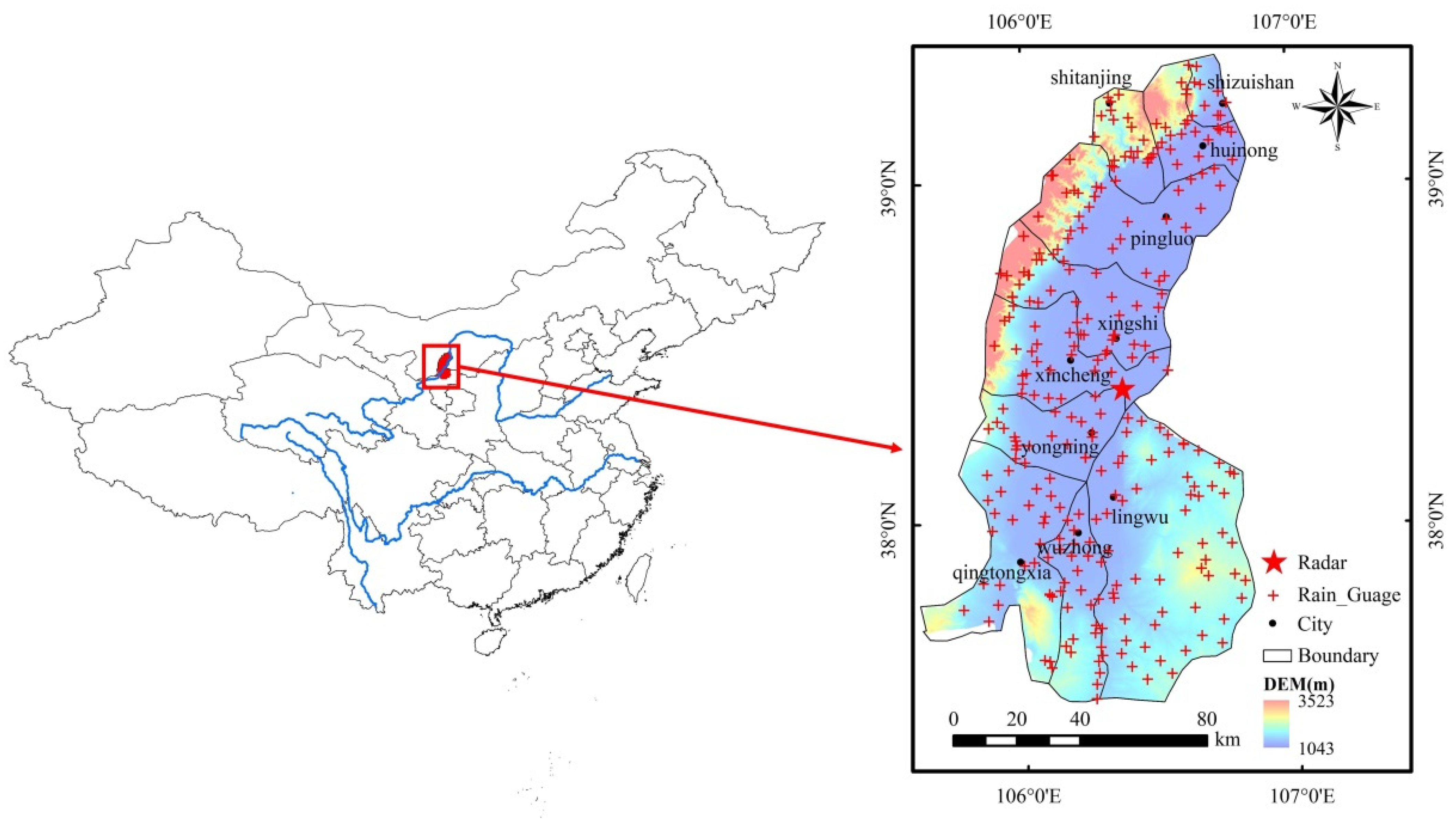
2.1. Study Area

The study area is located in Yinchuan city, Shizuishan city, and the surrounding areas in the Ningxia Hui Autonomous Region. The geographical distribution is shown in Figure 1. The geographical coordinates of the study area are located at 105°–108° E and 37°–40° N. The altitude is between 1000–3600 m, gradually decreasing from west to east, with the eastern foot of Helan Mountain in the northwest and the Yinchuan Plain in the central part.

According to the weather stations, the average annual temperature in the study area is 9.5 °C, with the lowest temperatures occurring in January and extreme lows below −22 °C. Annual sunshine hours range between 2800 and 3100 h, with average annual evaporation of 1890 mm and average annual precipitation of 171 mm, with June, July, August, and September accounting for 77% of the annual precipitation. The climate is characterized by windy and low rainfall, high evaporation, long sunshine hours, long winters and short summers, and large temperature differences between day and night. Due to the topography and subsurface, the eastern foothills of the Helan Mountains region are highly susceptible to extreme rainfall events [31]. Natural disasters such as flash floods, mudslides, and landslides caused by extreme rainfall have caused serious damage every year.

2.2. Data

As shown in

Table 1. Details of 10 rainfall events.

Event	Date	Start Time	Duration (hours)	Max Rain Rates (mm/h)	Average Rain Rates (mm/h)	Type	Note
1	12 April 2018	5:00	14	13.4	1.25	Stratiform	train
2	19 April 2018	10:00	15	28.4	1.87	Stratocumulus	train
3	18 May 2018	17:00	8	8	1.21	Stratiform	test
4	30 June 2018	19:00	24	37.6	2.37	Convective	train
5	22 July 2018	11:00	29	53	4.83	Convective	test
6	15 August 2018	9:00	41	25.2	1.23	Stratocumulus	train
7	26 April 2019	11:00	7	27.6	2.04	Stratocumulus	test
8	18 June 2019	23:00	39	3.4	0.49	Stratiform	test
9	11 September 2019	23:00	22	5.6	1.58	Stratiform	test
10	18 September 2019	12:00	10	3	0.57	Stratiform	train

, the rain gauge data in this study were derived from historical observations of 10 rainfall events collected in 2018–2019 at UTC. The geographical distribution of the rain gauges is shown in Figure 1, with a temporal resolution of 60 min and detection accuracy of 0.2 mm. The weather radar is a C-band Doppler weather radar from Yinchuan station in China’s New Generation Weather Radar (CINRAD) system, and the data time is consistent with the rain gauge time. The radar data is a 3D regularized grid product after quality control and interpolation. The radar data have a temporal resolution of approximately 6 min, a horizontal resolution of 1 km × 1 km, and a 3 km height layer selected in the vertical direction, with weaker reflectivity of less than 10 dBZ being disregarded.

The radar and rain gauge data should be matched to each other in time and space to build and evaluate the QPE algorithm more accurately. Firstly, the reflectivity factor Z at the corresponding grid point of the rain gauge is determined according to the time, latitude, and longitude of the rain gauge, ensuring that several reflectivity factor profiles are collected for each hour of the rain gauge. Secondly, the average value of the reflectivity factor Z at that grid point and the eight surrounding grid points at any given moment is obtained. Finally, the mean value is used as the radar-echo intensity value at the location of the rain gauge, thus constituting the radar-rain gauge database [32].

A total of 209 h of data were collected, and a database of 12,291 radar-rain gauges was established. As shown in Table 1, a total of 104 h of data from five rainfall events were selected to construct the QPE algorithm, and the remaining 105 h of data were used to test the performance of the algorithm.

3. Methodology

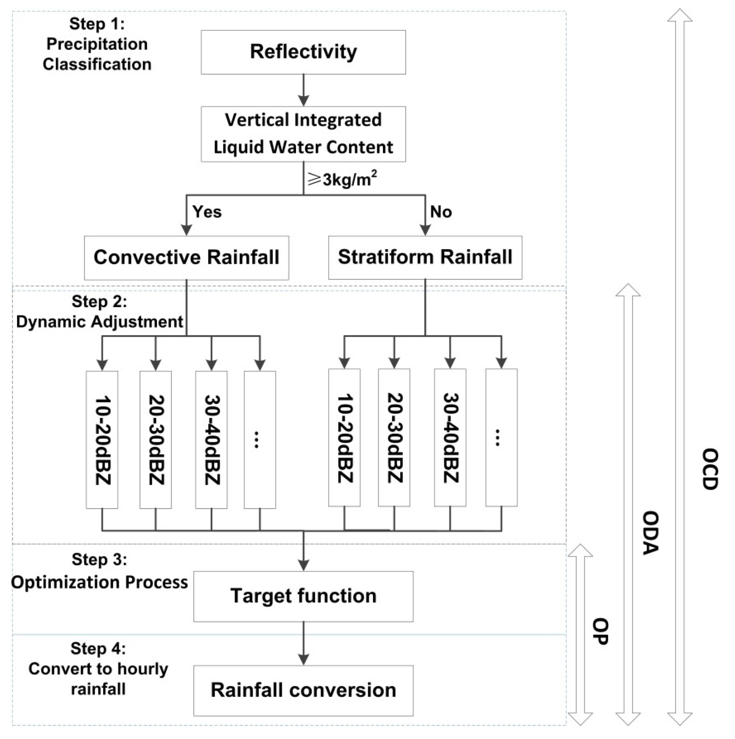
3.1. Optimization Process (OP)

Optimization Processes (OP) have achieved better results in fitting the Z-R relationship and have been widely used. In this study, the optimization method will be used to obtain the appropriate Z-R relationship. First, a Z-R relationship (Z = AR^b) is assumed, and a number of reflectivity factors in any hour are converted into radar-estimated rainfall Ri and integrated in time to obtain the hourly radar estimate Ri. Then, a Target Function (TF) is selected, the radar estimate Ri and rain gauge observation Gi at each point are substituted into the TF, and the parameters A and b in the Z-R relationship are adjusted by cycling. Finally, parameters A and b are optimal when the target discriminant function TF reaches its minimum value.

$$\mathrm{TF}=\min \left\{{{\displaystyle \int }}_{\mathrm{i}=1}^{\mathrm{n}}{{(\mathrm{R}}_{\mathrm{i}}-{\mathrm{G}}_{\mathrm{i}})}^2+\mid {\mathrm{R}}_{\mathrm{i}}-{\mathrm{G}}_{\mathrm{i}}\mid \right\}.$$

(1)

where n is the number of rain gauge-radar pairs, and i is their serial number. Parameters A and b are limited to take values in the range (10–1200) in steps of 0.1 and the parameter b in the range (0.5–5) in steps of 0.1 when performing numerical calculations to ensure the actual calculation efficiency.

3.2. Optimization Process of Dynamical Adjustment (ODA)

The variation of rainfall intensity is highly correlated with radar-echo intensity, and different radar-echo intensities may actually represent different rainfall intensities, so the corresponding Z-R relationship should be used in different radar-echo intensity ranges. First, the radar-rain gauge data pairs are divided into different intensity intervals using the hourly reflectivity factor average (dBZ_{hour_average}) in 10 dBZ intervals. Then, a set of Z-R relationships for the different intervals is calculated by OP. Finally, this set of Z-R relationships is used to obtain radar rainfall estimates.

The hourly reflectivity factor mean (dBZ_{hour_average}) is calculated as follows:

$${\mathrm{dBZ}}_{\mathrm{hour}\_\mathrm{average}}=\frac{{\mathrm{dBZ}}_{1 }{+\mathrm{dBZ}}_{2 }+\dots \dots {+\mathrm{dBZ}}_{\mathrm{n}}}{\mathrm{n}}.$$

(2)

where n is the number of radar reflectivity factors in hours. Compared to the full range of radar-echo intensity Z-R relationship optimization, this method divides the radar-echo intensity into multiple intervals to optimize the Z-R relationship and then uses OP to obtain the Z-R relationship in different radar-echo intensity ranges to improve the QPE accuracy.

3.3. Optimization Process of Precipitation Classification and Dynamical Adjustments (OCD)

Water vapor content is necessary for the production of clouds and precipitation. Dramatic changes in water vapor convergence often lead to disturbances in the spatial structure of the atmosphere and are an important driver for the occurrence and evolution of many catastrophic weather processes. The richer the water vapor content of the atmosphere, the more unstable it is, and the more unstable the atmosphere is prone to convective rainfall under the action of weather systems. Therefore, Vertically Integrated Liquid (VIL) in the atmosphere is an important indicator of the likelihood of convective rainfall [33].

Considering that radar reflectivity factors can be well-correlated with liquid water content, the use of reflectivity factors to differentiate between convective and stratified rainfall is a reasonable and convenient to implement method [34]. In this study, stratiform and convective rainfall are distinguished according to the magnitude of VIL. The Liquid Water (LW) is first calculated using Equation (3), and the VIL is obtained by doing the accumulation of LW in the vertical direction (Equation (4)). In order to better classify the radar-rain gauge data, it is stipulated that when the vertical liquid VIL is greater than 3 kg/m² at any time, the radar-rain gauge data in that hour is identified as convective precipitation. Otherwise, it is stratocumulus precipitation.

$$\mathrm{LW}=3{.44 \times 10}^3{\mathrm{Z}}^{4/7}$$

(3)

$$\mathrm{VIL}={{\displaystyle \sum }}_{\mathrm{i}=1}^{\mathrm{n}}{\mathrm{LW}}_{\mathrm{i}}{ \times \mathrm{DB}}_{\mathrm{i}}.$$

(4)

where DB is the altitude (km) at which the reflectivity factor is located, VIL is in kg/m² [34], and n is the altitude layer of the radar data. Through the above operations, radar-rain gauge data under convective and stratiform rainfall types can be obtained. Then ODA is used to complete the dynamic adjustment and optimization processes for the two types of rainfall separately, and finally, a QPE algorithm combining the Optimization process of precipitation Classification and Dynamical adjustments (OCD) can be established.

Figure 2 gives a schematic diagram of the processes of OCD, ODA, and OP. It can be seen that OCD actually uses two classification methods, automatic rainfall type recognition classification, and dynamic adjustment, and combines them with an Optimization Process (OP) to create the QPE algorithm.

3.4. Evaluation Indicators

The Correlation Coefficient (CC) is used to reflect the closeness of the correlation between radar rainfall values and rain gauge observations.

$$\mathrm{CC}=\frac{{{\displaystyle \sum }}_{\mathrm{i}=1}^{\mathrm{m}}{{\displaystyle \sum }}_{\mathrm{j}=1}^{\mathrm{n}}\left({\mathrm{R}}_{\left(\mathrm{i},\mathrm{j}\right)}-\stackrel{-}{{\mathrm{R}}_{\mathrm{i}}}\right)\left({\mathrm{G}}_{\left(\mathrm{i},\mathrm{j}\right)}-\stackrel{-}{{\mathrm{G}}_{\mathrm{i}}}\right)}{\sqrt{{{\displaystyle \sum }}_{\mathrm{i}=1}^{\mathrm{m}}{{\displaystyle \sum }}_{\mathrm{j}=1}^{\mathrm{n}}{\left({\mathrm{R}}_{\left(\mathrm{i},\mathrm{j}\right)}-\stackrel{-}{{\mathrm{R}}_{\mathrm{i}}}\right)}^2{\left({\mathrm{G}}_{\left(\mathrm{i},\mathrm{j}\right)}-\stackrel{-}{{\mathrm{G}}_{\mathrm{i}}}\right)}^2}}$$

(5)

R(i, j) is the jth radar estimate at time i, and G(i, j) is the corresponding surface rain gauge observation; m is the total number of rainfall hours involved in the assessment, and n is the total number of rain gauges involved in the assessment. The range of values for CC is [−1, 1]. Larger values indicate that the radar estimate is closer to the rain gauge observation and the algorithm is more effective. Otherwise, they are less similar.

Bias Ratio (BIAS) evaluates the difference in total rainfall by calculating the ratio of the total radar estimate to the total rain gauge observation. The closer the BIAS is to one, the closer the radar estimate is to the rain gauge observation. Greater than one indicates an overestimate of the radar, while less than one indicates an underestimate of the apparent radar.

$$\mathrm{BIAS}=\frac{{{\displaystyle \sum }}_{\mathrm{i}=1}^{\mathrm{m}}{{\displaystyle \sum }}_{\mathrm{j}=1}^{\mathrm{n}}{\mathrm{R}}_{\left(\mathrm{i},\mathrm{j}\right)}}{{{\displaystyle \sum }}_{\mathrm{i}=1}^{\mathrm{m}}{{\displaystyle \sum }}_{\mathrm{j}=1}^{\mathrm{n}}{\mathrm{G}}_{\left(\mathrm{i},\mathrm{j}\right)}}$$

(6)

Mean Absolute Error (MAE) indicates the mean value of the absolute error between the radar estimate and the rain gauge observation. The lower the MAE value, the lower the error between the radar estimate and the rain gauge observation.

$$\mathrm{MAE} = \frac{1}{\mathrm{m}\times \mathrm{n}}{{\displaystyle \sum }}_{\mathrm{i} = 1}^{\mathrm{m}}{{\displaystyle \sum }}_{\mathrm{j} = 1}^{\mathrm{n}}\left|{\mathrm{R}}_{(\mathrm{i},\mathrm{j})}-{\mathrm{G}}_{(\mathrm{i},\mathrm{j})}\right|$$

(7)

Root Mean Square Error (RMSE) measures the deviation between the observed value and the rain gauge observation.

$$\mathrm{RMSE} = \sqrt{\frac{1}{\mathrm{m}\times \mathrm{n}}{{\displaystyle \sum }}_{\mathrm{i} = 1}^{\mathrm{m}}{{\displaystyle \sum }}_{\mathrm{j} = 1}^{\mathrm{n}}{\left({\mathrm{R}}_{(\mathrm{i},\mathrm{j})}-{\mathrm{G}}_{(\mathrm{i},\mathrm{j})}\right)}^2}$$

(8)

4. Results and Discussion

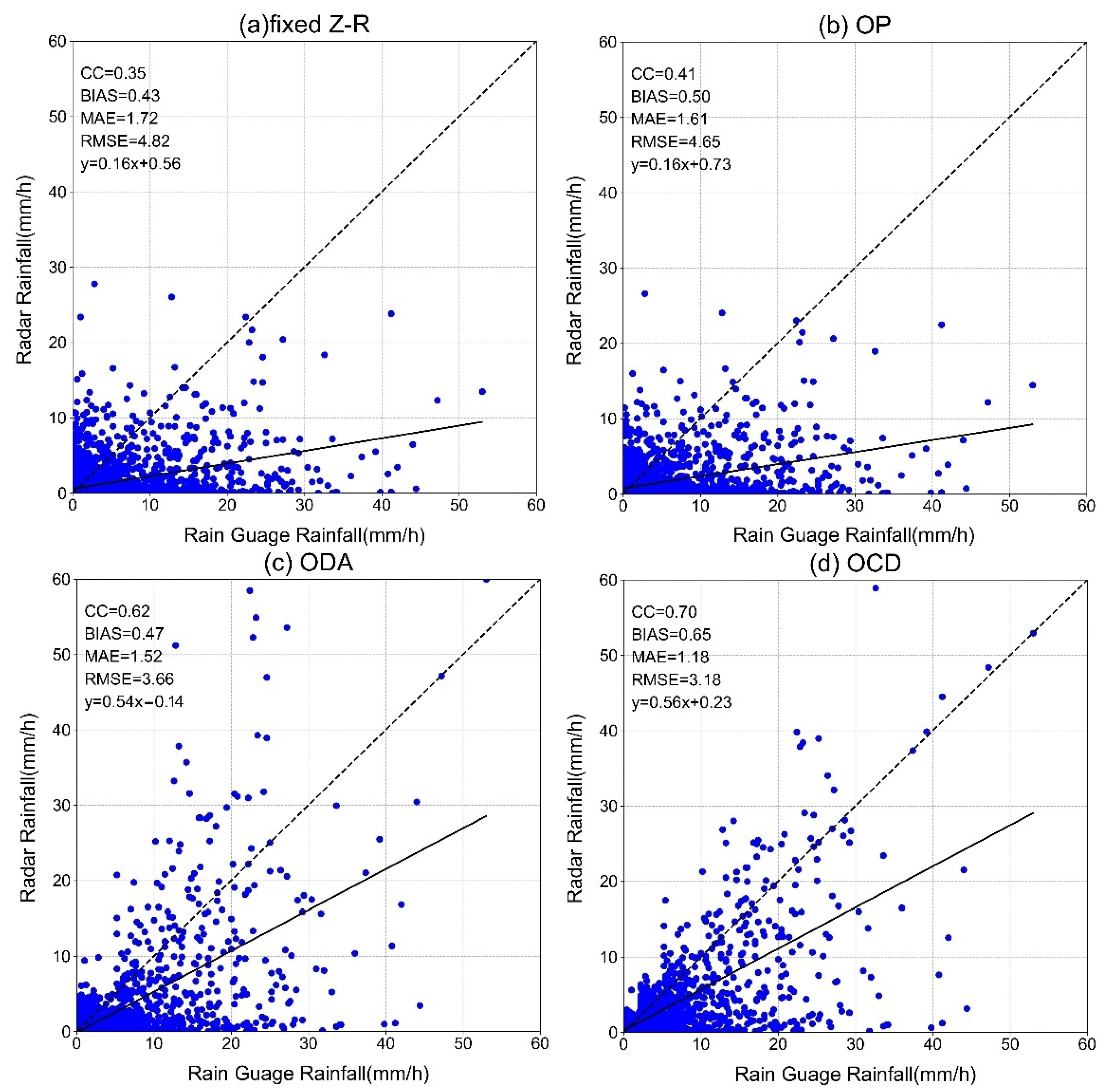
4.1. Scatter Distribution of Inversion Results by Algorithms

The results for the fixed Z-R relationship, OP, ODA, and OCD on the test set are given in Figure 3. It can be seen that compared to the fixed Z-R relationship, OP improves the estimation of rain gauge observations, with the CC improving from 0.35 to 0.41, MAE decreasing from 1.72 to 1.61, and RMSE decreasing from 4.82 to 4.65. The scatter distribution of OP is loose and not significantly regular. There is no significant change compared to the fixed Z-R relationship, and the improvement effect of OP is not significant. The number of samples with anomalously high or low OP is very large, with most of the data lying below the 45° line and the slope of the fitted curve slope k being 0.16. The OP has a significant underestimation of rainfall.

Compared to the fixed Z-R relationship and OP, both ODA and OCD show good improvements in all assessment indicators, with OCD achieving 0.7 and 0.65 for CC and BIAS, respectively, and 31% and 34% reductions in MAE and RMSE, respectively, all of which are better than ODA. The results of OCD have a greater linear relationship with rain gauge observations. Most of the sample data can be evenly distributed on both sides of the 45° line, and the rainfall estimates are better.

Overall, both OCD and ODA are effective in improving QPE accuracy, with ODA having better rainfall estimation and being more trusted and used. This is because ODA takes into account the physical characteristics of the radar echoes, classifies the rainfall, and classifies the reflectivity factor of the sample data before fitting the Z-R relationship, thus, significantly improving the rainfall estimation.

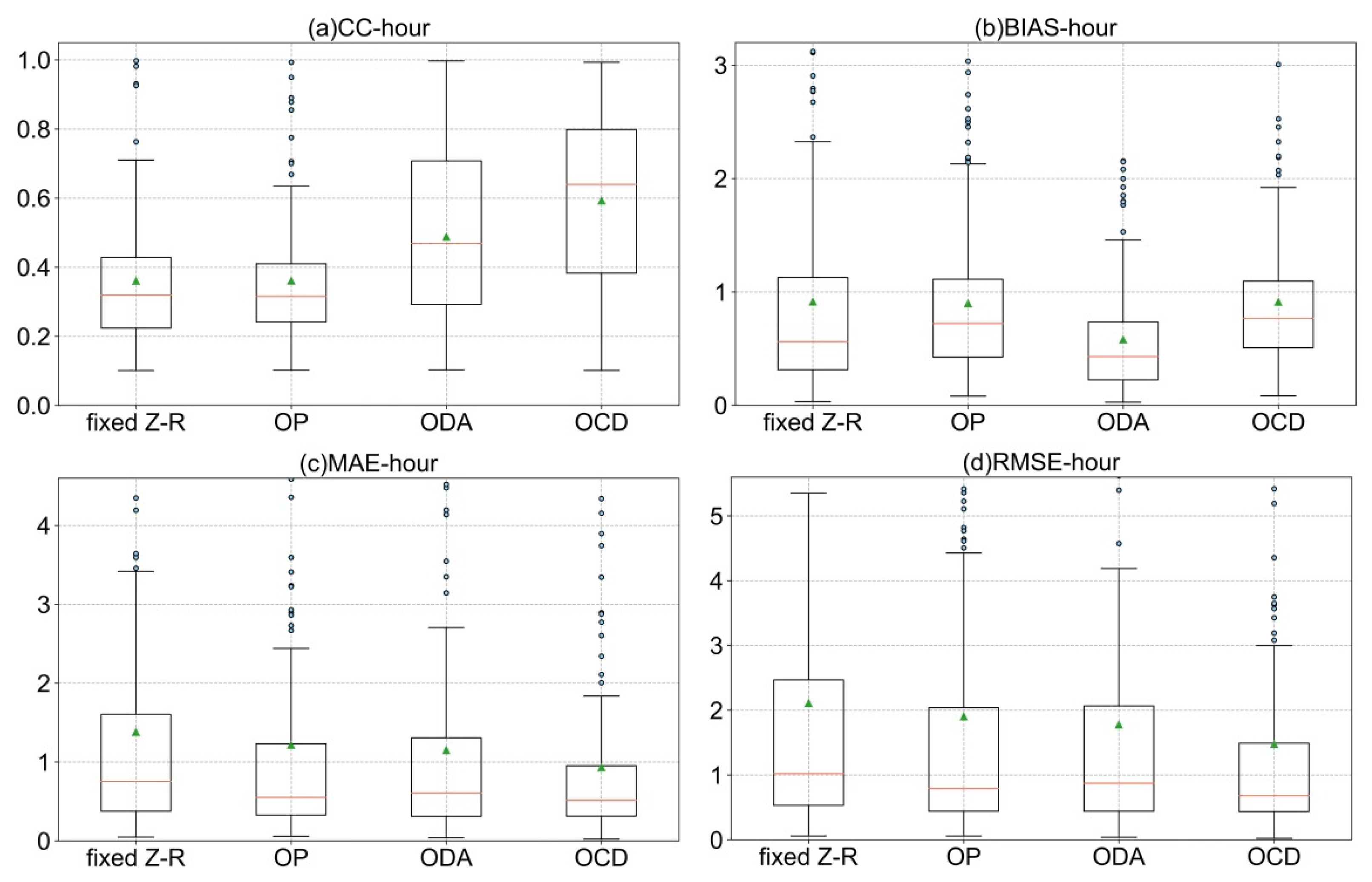
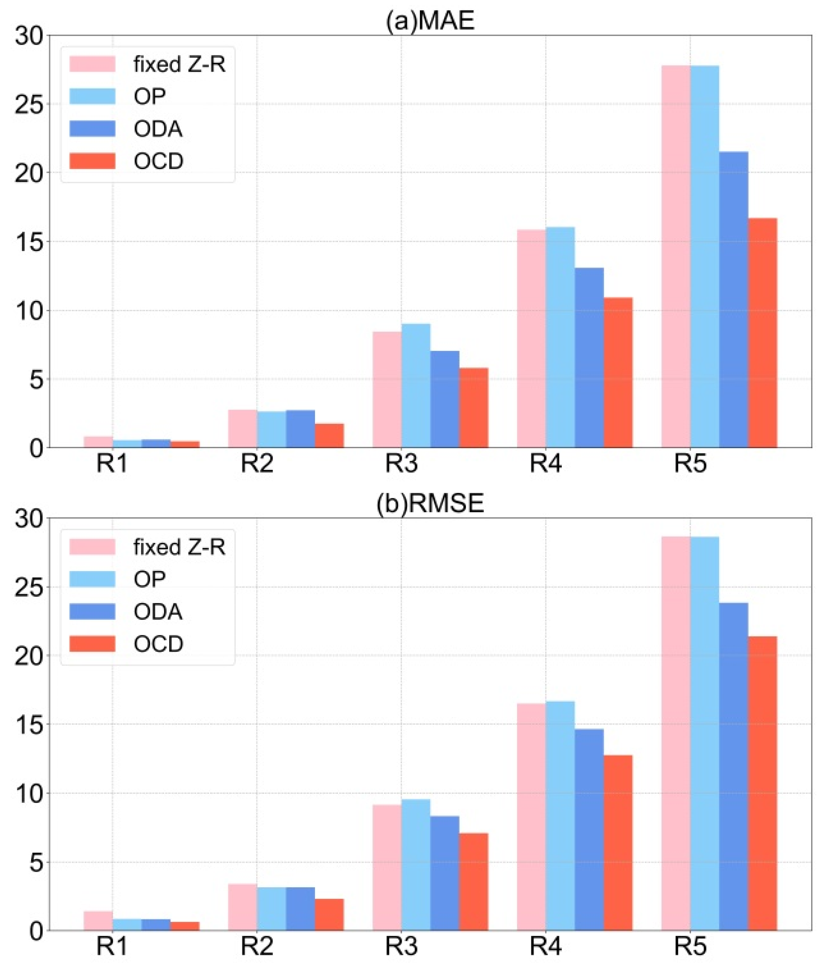
4.2. Evaluation Indicators Distribution of the Algorithms

Figure 4 gives the distribution of fixed Z-R relationship, OP, ODA, and OCD for each evaluation metric in the test set (105 h). For each box, the center of the box indicates the mean, the horizontal line indicates the median, and the top and bottom edges of the box are the 25th and 75th percentiles. For most of the fixed Z-R relationships and OP, the CCs were in the range of 0.2–0.4, while the CC for ODA and OCD were largely in the range of 0.4–0.8, with the mean and median for OCD, in particular, remaining around 0.6, indicating that the results for ODA and OCD were more stable and reliable. For BIAS, all four algorithms have more outliers, with OCD having the best results, with BIAS mostly staying between 0.5–1.1 and a median of 0.71. The fixed Z-R relationship and OP have the next best performance, with BIAS distributed between 0.3–1.1. OP has the worst results, with BIAS mainly distributed between 0.3–0.7, indicating that the rainfall underestimation of OP. The phenomenon is very obvious.

For MAE and RMSE, the mean and median values of OCD are the lowest, with OCD being more concentrated in the lower areas, indicating that OCD has the lowest error and demonstrates good rainfall estimation ability. This suggests that the uncertainty in ODA is somewhat higher, which may be due to the fact that some of the higher or lower radar reflectivity factors do not match well with their corresponding surface rainfall when the radar reflectivity factor is graded, resulting in biased rainfall estimates. For the fixed Z-R relationship, the MAE and RMSE perform the least well, with a relatively wide distribution range along with the highest mean and median values, suggesting that fixed Z-R introduces significant bias in rainfall estimates.

4.3. Performance of Algorithms under Different Rain Rates

To better investigate the fixed Z-R relationship, we examined the performance of OP, ODA, and OCD under different rain rates (RR). The data in the test set were classified into samples according to R1 (0.2 ≤ RR < 2.5 mm/h), R2 (2.5 ≤ RR < 8 mm/h), R3 (8 ≤ R < 16 mm/h), R4 (16 ≤ RR < 25 mm/h) and R5 (25 mm/h ≤ RR). The results of MAE and RMSE for different algorithms for the five scenarios are shown in Figure 5.

It can be seen that the MAE and RMSE of ODA and OCD are both lower than the fixed Z-R relationship and OP under different rain rates, with the MAE and RMSE of OCD being significantly lower than those of ODA, indicating that OCD has better stability and better rainfall estimation capability under different rain rates. The results of ODA are not so obvious, especially for weaker rainfall (R1 and R2), and the estimation ability of ODA for weaker rainfall needs to be further improved.

OP has a fair estimation capability for weaker rainfall (R1 and R2), with both MAE and RMSE slightly lower than the fixed Z-R relationship, but both MAE and RMSE for stronger rainfall (R3, R4, and R5) are higher for OP than the fixed Z-R relationship, indicating that OP leads to greater errors. This is due to the fact that the OP will focus more on the optimum in the presence of a large amount of weaker rainfall data during the search for parameters A and b and ignore the stronger rainfall data, which is eventually reflected in the OP’s wrong estimation of the stronger rainfall. In practical operational work, one would prefer to obtain optimal estimates of stronger rainfall rather than weaker rainfall, and the inappropriate use of OP may exacerbate this phenomenon.

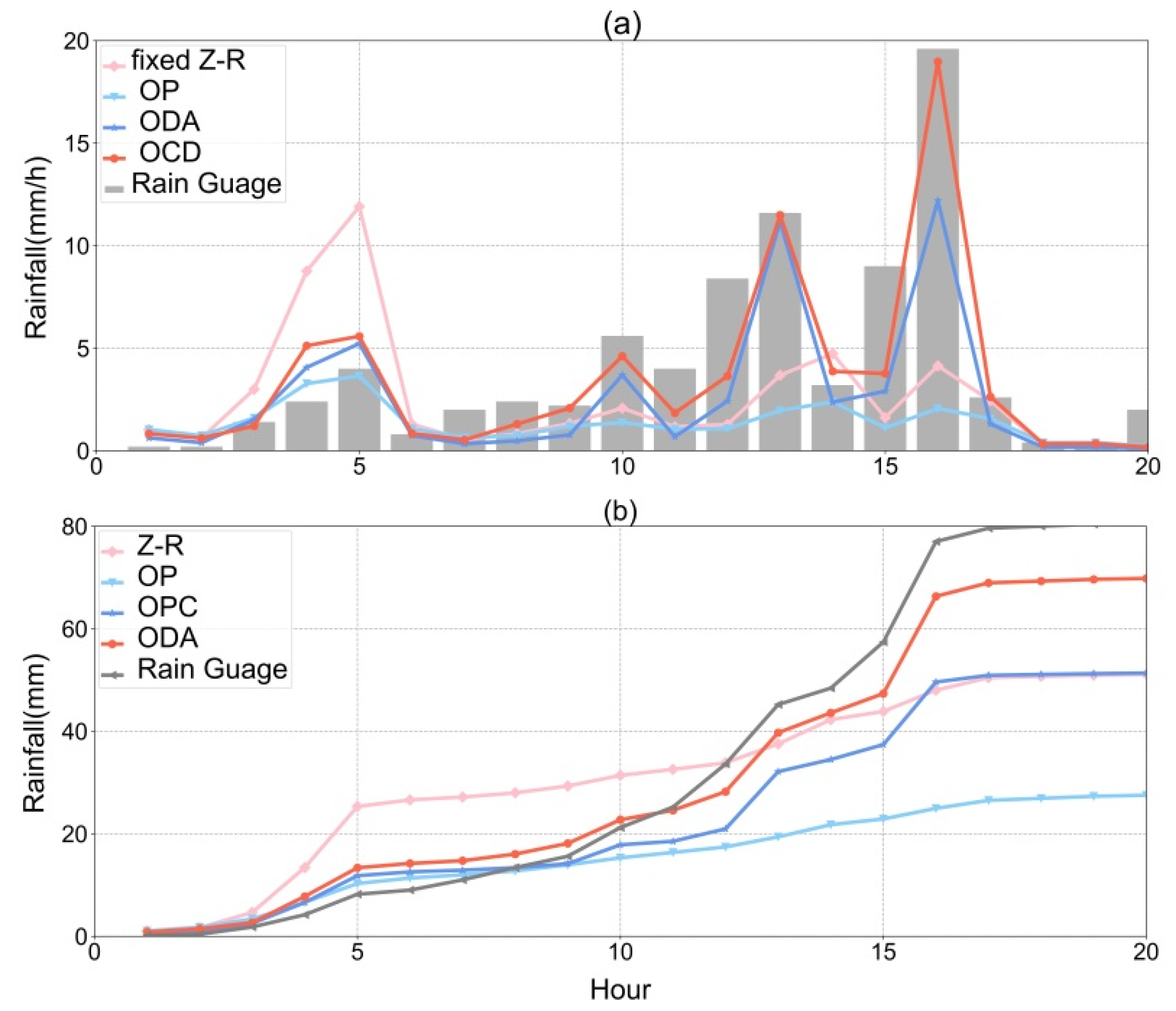
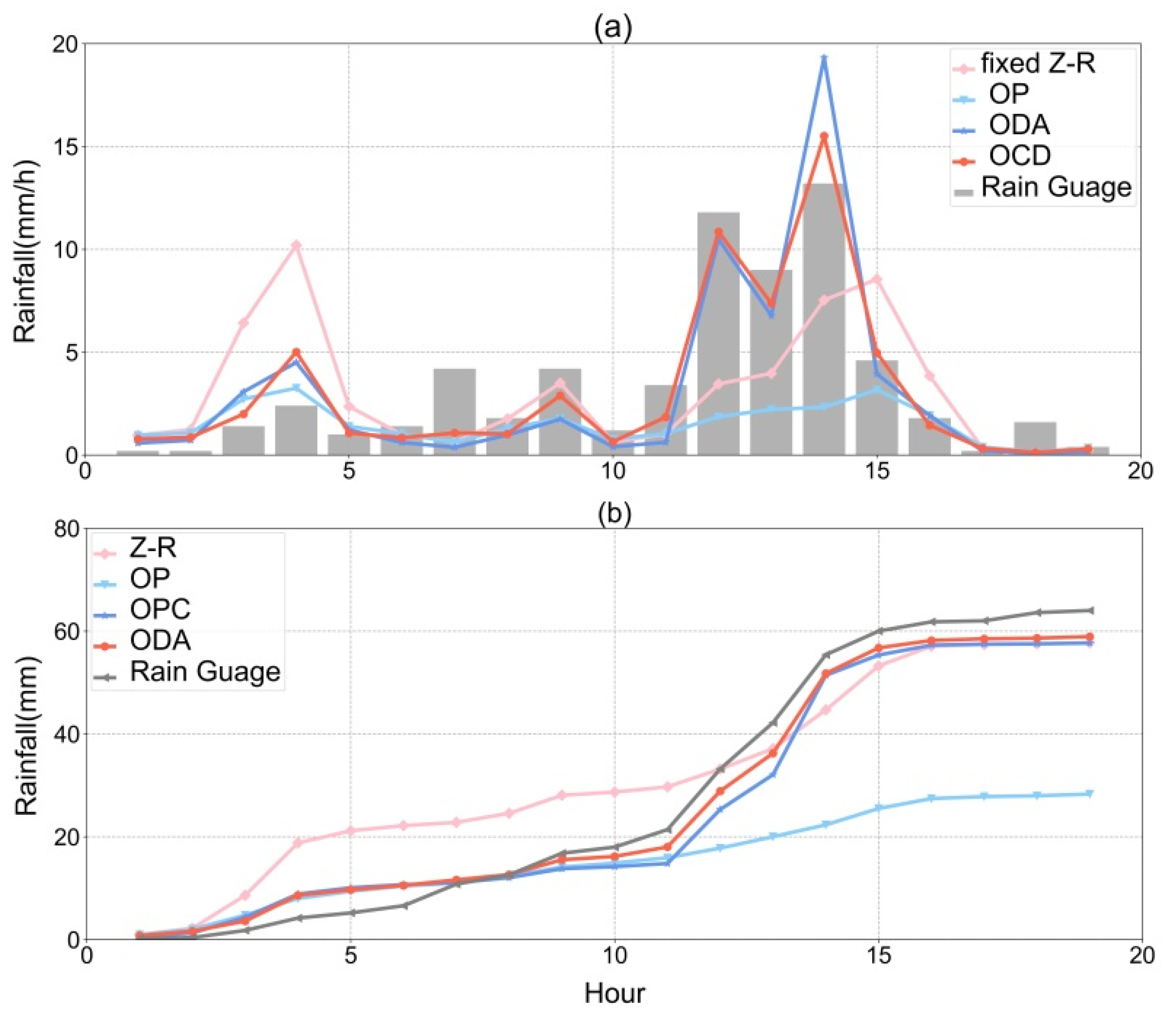
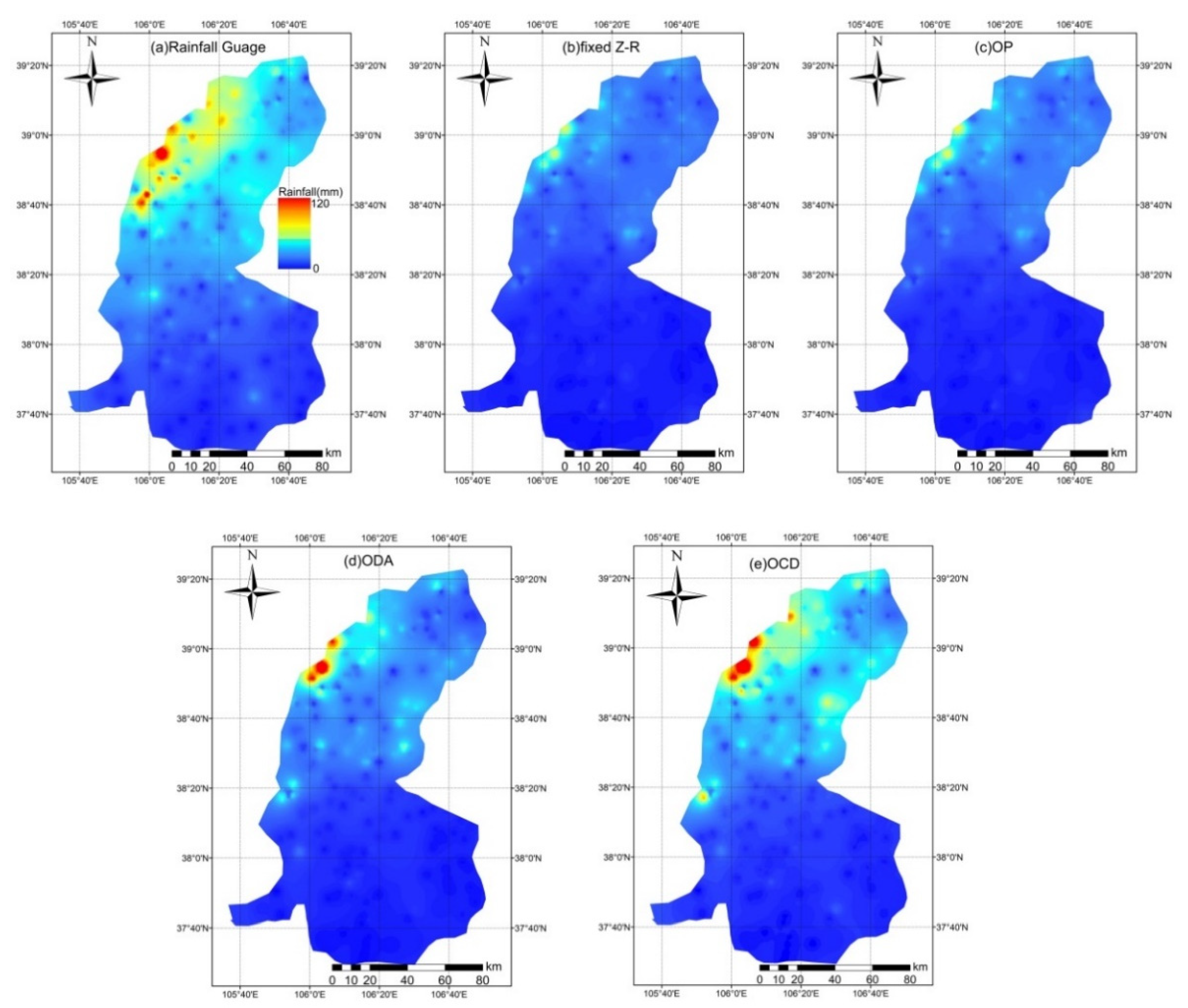
4.4. Case Analysis of Rainfall Event

Studying the hourly evolution characteristics of different QPE algorithms in rainfall events can intuitively evaluate the performance of QPE algorithms. Therefore, two rain gauges with longer recorded data during a convective rainfall event (22 July 2018, number 5) were selected to carry out an evaluation of the effect of fixed Z-R relationship, OP, ODA, and OCD, and the results are shown in Figure 6 and Figure 7.

As can be seen from Figure 6a, the actual rain rates at the beginning of the rainfall process (1–5 h) are all below 5 mm/h, but the fixed Z-R relationship produces an anomalous overestimation of rainfall, corresponding to a very significant change in the cumulative rainfall curve at this time in Figure 6b. In contrast, by the middle and late stages of the rainfall process (12–16 h), the fixed Z-R relationship produces a much lower estimate of strong rainfall than the rain gauge. Similar results are clearly shown in Figure 7a for another rain gauge, where the fixed Z-R relationship is estimated to be 10 mm for 2 mm of rainfall at 4 h, and the false underestimation of strong rainfall is also very evident later in the rainfall process. This suggests that the fixed Z-R relationship overestimates rainfall at low rain rates and underestimates it at higher rain rates.

OP is relatively close to the rain gauge observations at the beginning of the rainfall process and fits well with the changes in the cumulative rainfall curve, with the OP achieving better results at lower rain rates. However, in the middle and late stages of the rainfall process, OP estimates deviate extremely remarkably, even exceeding the fixed Z-R relationship. This indicates that OP does not capture the variability of strong rainfall well, which better validates the analysis in Section 4.3 that OP has a poor ability to estimate strong rainfall.

As can be seen from Figure 6 and Figure 7, the ODA and OCD rainfall estimates for different periods are significantly less biased than the fixed Z-R relationship and OP, with no abnormal overestimation or underestimation, and the cumulative rainfall curves are closer to the rain gauge observations, indicating that ODA and OCD have more stable and accurate rainfall estimation capabilities. In the middle and late stages of rainfall, ODA is more biased at some points, while OCD is closer to the rain gauge observations, indicating that OCD has a better estimate of strong rainfall and demonstrating the importance of precipitation classification.

Overall, ODA and OCD can effectively improve the accuracy and stability of OP by further combining precipitation classification and dynamical adjustment methods, especially OCD is more capable of estimating strong rainfall events. However, all four algorithms produce different degrees of underestimation of the final cumulative rainfall, with OCD, which has the best rainfall estimation capability, also underestimating 12.6% and 7.4% of the rainfall, and further improvement of the algorithms is expected in subsequent work.

Radar Quantitative Precipitation Estimate can better reflect the spatial distribution characteristics of rainfall, which is one of the advantages of radar equipment detection, and the description of spatial rainfall distribution by radar rainfall is also an important component in the assessment of the effectiveness of radar rainfall inversion. Therefore, the inverse distance weighting method was used to spatially interpolate the accumulated rainfall observed by the rain gauge, and the results obtained were used as the true rainfall field and compared with the fixed Z-R relationship, OP, ODA, and OCD, to analyze the advantages and disadvantages of the four algorithms in describing the spatial distribution of regional accumulated rainfall, and the results are shown in Figure 8.

Firstly, it can be seen that the regional cumulative rainfall shows a distribution characteristic of gradually increasing from south to north, and the area of strong rainfall is mainly distributed around the eastern foothills of the Helan Mountains (38°40′–39°20′ N, 106°–106°20′ E), with the cumulative rainfall in most areas exceeding 100 mm. The fixed Z-R relationship and OP do not portray the central distribution of strong rainfall well. OCD and ODA provide a significant improvement in the regional distribution and magnitude of strong rainfall, as well as a better description of the local characteristics of rainfall distribution.

ODA further demonstrates the advantages of ODA by providing a better and more accurate estimate of the overall spatial distribution of rainfall, although it does not reflect the distribution of a small proportion of strong rainfall overall.

5. Conclusions

The purpose of this study is to construct a dynamic Z-R relationship based on precipitation classification to improve the accuracy of QPE, and a comparative study with some existing QPE algorithms is conducted, with the following main findings.

OP can improve the QPE errors brought about by the fixed Z-R relationship, but the improvement is not significant (MAE and RMSE are reduced by 6% and 3%, respectively). OP has a large number of abnormally high or abnormally low data, which significantly underestimates rainfall. ODA and OCD significantly reduce the QPE error, with OCD being the best estimate, achieving a CC of 0.7 and a 31% and 34% reduction in MAE and RMSE, respectively.

For hourly CC and BIAS, OCD concentrates the distribution in a more reasonable interval, with both mean and median significantly better than other QPE algorithms. The distribution of BIAS for ODA concentrates in the range of 0.3–0.6, which is worse than the fixed Z-R relationship and OP, indicating higher uncertainty for ODA. For both hourly MAE and RMSE, OCD is concentrated in the region of lower values, which indicates that OCD has the lowest error and OCD is the more reliable algorithm.

The MAE and RMSE of both ODA and OCD are lower than those of the fixed Z-R relationship and OP for different rain rates, with the MAE and RMSE of OCD being significantly lower than those of ODA, indicating that OCD has better stability and QPE capability. The estimation capability of OP for weaker rainfall is fair, but the estimation error of OP for stronger rainfall is higher than that of the fixed Z-R relationship. This is due to the fact that the OP may fall into a local optimum during the search for parameters A and b. The OP will focus more on the optimum, where there is a large amount of weaker rainfall, and ignore the stronger rainfall.

If fixed the Z-R relationship will produce the overestimation for stronger rainfall and the underestimation for weaker rainfall. The OP will not capture the variability of stronger rainfall well and will underestimate rainfall even more incorrectly for stronger rainfall. OCD is the best-performing of the four QPE algorithms in terms of accuracy and stability, and the distribution and magnitude of strong rainfall areas are significantly improved for both OCD and ODA. Both have improved more significantly, with OCD having a better description of the local characteristics of the rainfall distribution, further reflecting the advantages of ODA. However, four QPE algorithms produce different degrees of underestimation of cumulative rainfall, and we will also further improve the capabilities of the algorithms in subsequent work.

References

1. Andersen, C.T.; Foster, I.D.L.; Pratt, C.J. The role of urban surfaces (permeable pavements) in regulating drainage and evaporation: Development of a laboratory simulation experiment. Hydrol. Process. 2015, 13, 597–609. [Google Scholar] [CrossRef]
2. Zhou, Y.; Smith, S.J.; Zhao, K.; Imhoff, M.; Thomson, A.; Bond-Lamberty, B.; Asrar, G.R.; Zhang, X.; He, C.; Elvidge, C.D. A global map of urban extent from nightlights. Environ. Res. Lett. 2015, 10, 054011. [Google Scholar] [CrossRef]
3. Goudenhoofdt, E.; Delobbe, L. Evaluation of radar-gauge merging methods for quantitative precipitation estimates. Hydrol. Earth Syst. Sci. 2009, 13, 195–203. [Google Scholar] [CrossRef] [Green Version]
4. Yang, L.; Tian, F.; Smith, J.A.; Hu, H. Urban signatures in the spatial clustering of summer heavy rainfall events over the Beijing metropolitan region. J. Geophys. Res. Atmos. 2014, 119, 1203–1217. [Google Scholar] [CrossRef]
5. Ochoa-Rodriguez, S.; Wang, L.P.; Willems, P.; Onof, C. A Review of Radar-Rain Gauge Data Merging Methods and Their Potential for Urban Hydrological Applications. Water Resour. Res. 2019, 55, 6356–6391. [Google Scholar] [CrossRef]
6. Berne, A.; Krajewski, W.F. Radar for hydrology: Unfulfilled promise or unrecognized potential? Adv. Water Resour. 2013, 51, 357–366. [Google Scholar] [CrossRef]
7. Auipong, N.; Trivej, P. Study of Z-R relationship among different topographies in Northern Thailand. J. Phys. Conf. Ser. 2018, 1144, 012098. [Google Scholar] [CrossRef]
8. Marshall, J.S.; Palmer, W. The Distribution of Raindrops With Size. J. Meteor. 1948, 5, 165–166. [Google Scholar] [CrossRef]
9. Vieux, B.E.; Bedient, P.B. Estimation of Rainfall for Flood Prediction from WSR-88D Reflectivity: A Case Study, 17–18 October 1994. Weather Forecast. 1998, 13, 407–415. [Google Scholar] [CrossRef]
10. Fulton, R.A.; Breidenbach, J.P.; Seo, D.J.; Miller, D.A.; O’Bannon, T. The WSR-88D Rainfall Algorithm. Weather Forecast. 1997, 13, 377–395. [Google Scholar] [CrossRef]
11. Ciach, G.J.; Krajewski, W.F. Radar-Rain Gauge Comparisons under Observational Uncertainties. J. Appl. Meteorol. 1998, 38, 1519–1525. [Google Scholar] [CrossRef]
12. Ulbrich, C.W.; Lee, L.G. Rainfall Measurement Error by WSR-88D Radars due to Variations in Z–R Law Parameters and the Radar Constant. J. Atmos. Ocean. Technol. 1999, 16, 1017–1024. [Google Scholar] [CrossRef]
13. Kato, A.; Maki, M. Localized Heavy Rainfall Near Zoshigaya, Tokyo, Japan on 5 August 2008 Observed by X-band Polarimetric Radar—Preliminary Analysis—. Sola 2009, 5, 89–92. [Google Scholar] [CrossRef] [Green Version]
14. Atlas, D.; Rosenfeld, D.; Wolff, D.B. Climatologically tuned reflectivity-rain rate relations and links to area-time integrals. J. Appl. Meteorol. 1990, 29, 1120–1135. [Google Scholar] [CrossRef]
15. Xu, Z.F.; Xiong, J.; Ge, W.Z. Application of Genetic Algorit h min Optimizing the Z-R Parameter to Radar Rainfall Estimati on. Plateau Meteorol. 2006, 4, 710–715. [Google Scholar]
16. Zhang, Y.; Yang, J.; Zhang, W.Q. Study on modification to optimization method of Z-I relationship. J. Meteorol. Environ. 2015, 31, 97–102. [Google Scholar]
17. Chapon, B.; Delrieu, G.; Gosset, M.; Boudevillain, B. Variability of rain drop size distribution and its effect on the Z–R relationship: A case study for intense Mediterranean rainfall. Atmos. Res. 2008, 87, 52–65. [Google Scholar] [CrossRef]
18. Balakrishnan, N.; Zrnić, D.S.; Goldhirsh, J.; Rowland, J. Comparison of Simulated Rain rates from Disdrometer Data Employing Polarimetric Radar Algorithms. J. Atmos. Ocean. Technol. 1989, 6, 476–486. [Google Scholar] [CrossRef]
19. Uijlenhoet, R.; Steiner, M.; Smith, J.A. Variability of Raindrop Size Distributions in a Squall Line and Implications for Radar Rainfall Estimation. J. Hydrometeorol. 2003, 4, 43–61. [Google Scholar] [CrossRef]
20. Ulbrich, C.W.; Atlas, D. On the Separation of Tropical Convective and Stratiform Rains. J. Appl. Meteorol. 2002, 41, 188–195. [Google Scholar] [CrossRef]
21. Steiner, M.; Houze, R.A., Jr.; Yuter, S.E. Climatological characterization of three-dimensional storm structure from operational radar and rain gauge data. J. Appl. Meteorol. Climatol. 1995, 34, 1978–2007. [Google Scholar] [CrossRef]
22. Chumchean, S.; Sharma, A.; Seed, A. An Integrated Approach to Error Correction for Real-Time Radar-Rainfall Estimation. J. Atmos. Ocean. Technol. 2006, 23, 67–79. [Google Scholar] [CrossRef]
23. Zhang, J.; Langston, C.; Howard, K. Brightband Identification Based on Vertical Profiles of Reflectivity from the WSR-88D. J. Atmos. Ocean. Technol. 2008, 25, 1859–1872. [Google Scholar] [CrossRef]
24. Howard, K.; Zhang, J. Multi-sensor QPE in the National Mosaic and QPE (NMQ) System. AGU Spring Meet. Abstr. 2007, 2007, H52A-04. [Google Scholar]
25. Alfieri, L.; Claps, P.; Laio, F. Time-dependent Z-R relationships for estimating rainfall fields from radar measurements. Nat. Hazards Earth Syst. Sci. 2010, 10, 149–158. [Google Scholar] [CrossRef] [Green Version]
26. Crosson, W.L.; Duchon, C.E.; Raghavan, R.; Goodman, S.J. Assessment of rainfall estimates using a standard ZR relationship and the probability matching method applied to composite radar data in central Florida. J. Appl. Meteorol. Climatol. 1996, 35, 1203–1219. [Google Scholar] [CrossRef]
27. Wang, Y.; Feng, Y.; Cai, J.; Hu, S. An approach for radar quantitative precipitation estimate based on categorical ZI relations. J. Trop. Meteorol. 2011, 27, 601–608. [Google Scholar]
28. Gou, Y.B.; Liu, L.; Wang, D.; Zhong, L.; Chen, C. Evaluation and Analysis of the Z-R Storm-Grouping Relationships Fitting Scheme based on Storm Identification. Torrential Rain Disasters 2015, 34, 1–8. [Google Scholar]
29. Duan, Y.; Wang, G.; Zhi, S.; Ling, T.; Fu, W.B. Area Rainfall Estimation Based on Cloud Grouping Z-R Relationship Along Zhejiang Jiangxi Railway Lines. J. Arid Meteorol. 2019, 37, 972–978. [Google Scholar]
30. Wu, W.; Zou, H.; Shan, J.; Wu, S. A Dynamical Z-R Relationship for Precipitation Estimation Based on Radar Echo-Top Height Classification. Adv. Meteorol. 2018, 2018, 8202031. [Google Scholar] [CrossRef] [Green Version]
31. Li, S.; Wei, H.; Liu, Y.; Ma, W.; Gu, Y.; Peng, Y.; Li, C. Runoff prediction for Ningxia Qingshui River Basin under scenarios of climate and land use changes. Acta Ecol. Sin. 2017, 37, 1252–1260. [Google Scholar]
32. Yuan, X.Q.; Ni, G.H.; Pan, A.J. NEXRAD Z-R Power Relationship in Beijing Based on Optimization Algorithm. J. China Hydrol. 2010, 30, 1–6. [Google Scholar]
33. Houghton, H.G. On precipitation mechanisms and their artificial modification. J. Appl. Meteorol. Climatol. 1968, 7, 851–859. [Google Scholar] [CrossRef]
34. Qi, Y.; Zhang, J.; Zhang, P. A real-time automated convective and stratiform precipitation segregation algorithm in native radar coordinates. Q. J. R. Meteorol. Soc. 2013, 139, 2233–2240. [Google Scholar] [CrossRef]
Figure 1. Spatial map showing the elevation of the study area, together with rain gauges and weather radar.
Water 14 03436 g001
Figure 2. Flow diagram of the QPE algorithm.
Water 14 03436 g002
Figure 3. Scatter distribution of Rain Gauge Rainfall and different QPE algorithms, (a) fixed Z-R, (b) OP, (c) ODA and (d) OCD.
Water 14 03436 g003
Figure 4. The distribution of the evaluation indicators for fixed Z-R, OP, ODA, and OCD at hourly scales, (a) CC, (b) BIAS, (c) MAE, (d) RMSE.
Water 14 03436 g004
Figure 5. (a) MAE and (b) RMSE of fixed Z-R, OP, ODA, and OCD at different rain rates.
Water 14 03436 g005
Figure 6. Time-by-time evolutionary characteristics of 4 QPE algorithms (rainfall event 5, rain gauge ID: 40505780), (a) hourly, (b) cumulant.
Water 14 03436 g006
Figure 7. Time-by-time evolutionary characteristics of 4 QPE algorithms (rainfall event 5, rain gauge ID:40537250), (a) hourly, (b) cumulant.
Water 14 03436 g007
Figure 8. Spatial distribution of rainfall in 22 July 2018, (a) interpolation of rain gauge observations, (b) fixed Z-R for radar, (c) OP for radar, (d) ODA for radar and (e) OCD for radar.
Water 14 03436 g008