
Analytical Modeling with Laboratory Data and Observations of the Mechanisms of Backward Erosion Piping Development
1
School of Civil Engineering and Transportation, South China University of Technology, Guangzhou 510640, China
2
The State Key Laboratory of Subtropical Building Science, South China University of Technology, Guangzhou 510640, China
3
Department of Civil and Environmental Engineering, Utah State University, Logan, UT 84322, USA
*
Author to whom correspondence should be addressed.
Water 2022, 14(21), 3420; https://doi.org/10.3390/w14213420
Submission received: 31 August 2022
/
Revised: 11 October 2022
/
Accepted: 18 October 2022
/
Published: 27 October 2022
(This article belongs to the Section Soil and Water)
Abstract
:Backward erosion piping accounts for one of the leading threats to dams and levees throughout the world. A laboratory modeling program has been conducted to interpret pore pressure data and observations collected during backward erosion piping (BEP) initiation and progression in sandy soils. An analytical model has been applied to assess the development of BEP mechanisms as well as calculating the critical hydraulic conditions required for various BEP stages to initiate and progress. The results with the predicted model are produced by successively matching the hydraulic head regime surrounding the developing BEP stages based on observations and pore pressure measurements obtained from the laboratory models. Interpretation based on an analytical model allows assessment of the processes governing BEP initiation and progression, including: (1) substantial concentrations of seepage flow around the edge of the exit area resulting in increased gradients and BEP initiation (i.e., sand boiling); (2) soil particles collapsing leading to BEP progression (i.e., channel development). The findings of the study identified the criterion for governing channel progression that can be applied to the assessment of BEP mechanics.
1. Introduction
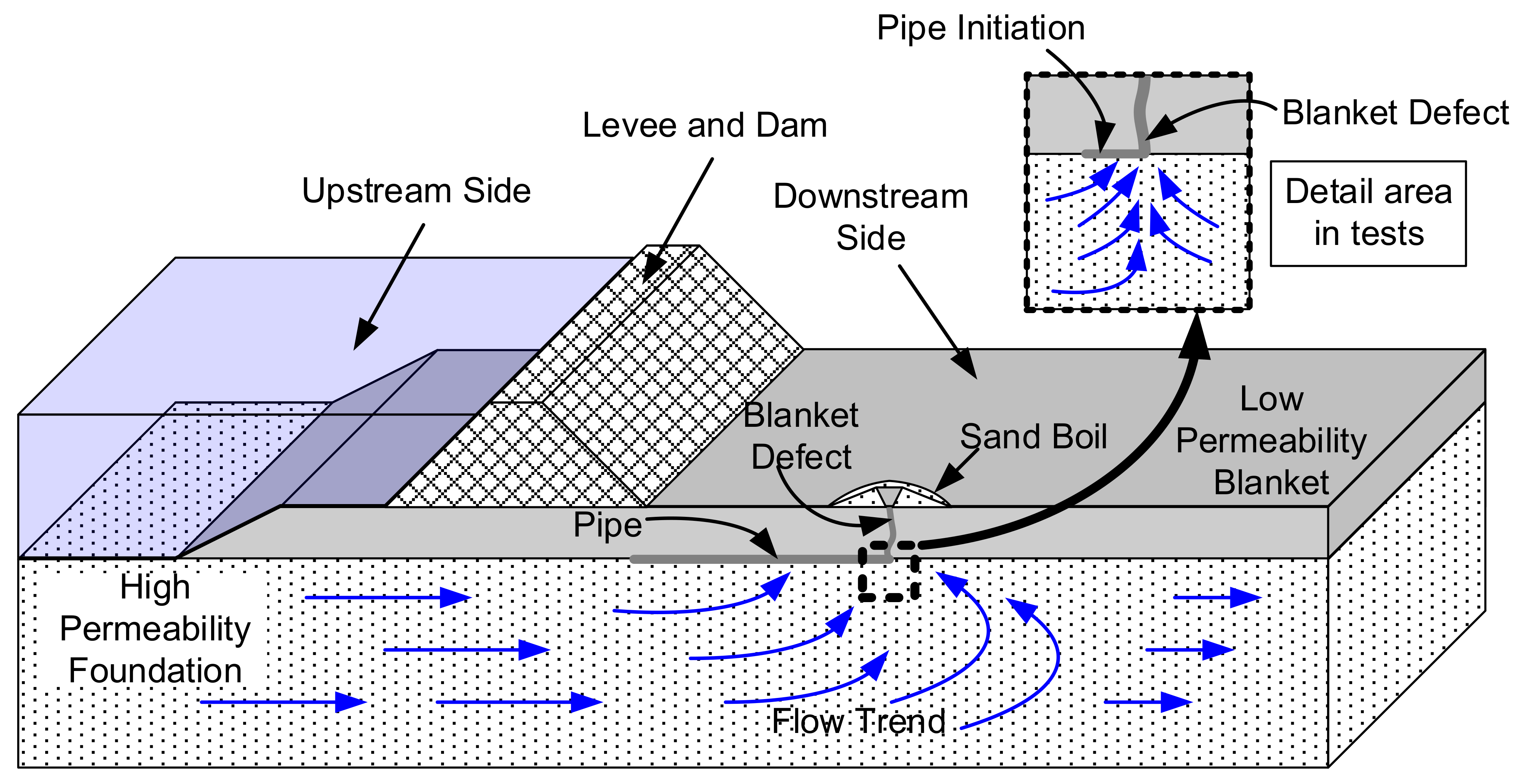
Backward erosion piping (BEP) is one of the least understood mechanisms of internal erosion observed in dams, levees, and their foundations. Internal erosion in its various forms can be attributed as one of the main causes of dam and levee failures worldwide [1,2]. BEP occurs with the removal of individual non-plastic soil particles out of a seepage exit point thus resulting in the formation of a “backward” progressing channel or pipe toward the seepage source.
Overview of BEP mechanism. A schematic interpretation of a condition where BEP frequently occurs through a defect in an overlying low-permeability layer is presented in Figure 1. The BEP mechanism consists of: (1) the formation of a loosened zone, (2) detachment of individual soil particles, (3) transportation of soil particles to an exit, and (4) the formation of one or several pipes. The loosened zone initially forms at the exit location and has been observed to progress with the developing erosion [3,4]. As the hydraulic gradient and total flows increase, the flow in the defect area starts carrying soil particles in suspension and the soil is “fluidized” [5,6,7]. Because the pipe is a path of least seepage resistance, the pressure loss and hydraulic gradient inside the piping path decrease, then seepage from the surrounding soil converges into the pipe and increases both the hydraulic gradient at the pipe head and the flow volume within the pipe. Therefore, the pipe now has more capacity to progress toward the flow source, forming an erosion pipe and uncontrolled erosion can lead to the potential collapse of the structure.
Background. Numerous investigations are based on laboratory testing by a number of researchers with the goal of observing the BEP mechanisms and quantifying the hydraulic driving forces needed to initiate and progress BEP. Sellmeijer and his co-workers from Delft Geotechnics Laboratories and Delft Hydraulics in the Netherlands performed a wide variety of BEP flumes tests on determining the critical hydraulic condition for BEP development across the water retention structure [8,9,10,11]. At the same time, Miesel and his co-workers from Germany conducted an extensive investigation for BEP processes [12,13,14]. Most experiments indicated that BEP can initiate at one differential head and then reach an equilibrium state without further BEP development, or a further increase in the differential head is needed for the pipe to lengthen (progression controlled). However, in some of the experiments, BEP can initiate at one differential head and then progress backward continuously towards the seepage source without reaching any equilibrium (initiation controlled) [15,16,17,18]. Schmertmann also studied BEP through a variety of experimental flumes for analyzing the critical heads needed for BEP initiation and progression [19]. The uniformity coefficient of the sand was found to play a significant role in the erosion potential.
Although these flume experiments focus on the behavior of progressing BEP, their main objective was to predict the critical hydraulic loading that was leading BEP initiation and progression to failure, the small-scale mechanisms occurring around the initiated point of erosion which play an important role in determining the progression, especially the controlled factors for initiated erosion, and how to propagate to channel initiation and development.
Several analytical predictive methods for determining the critical head have been developed to investigate the critical conditions that lead to BEP failure. Sellmeijer combined groundwater flow equations with equations for the micro-scale processes in the pipe (grain equilibrium and Poiseuille flow) [9]. The model was calibrated using large-scale experiments in the Delta flume and recently adapted on the basis of the results of additional experiments [10,20]. Hoffmans deduced the Shields–Darcy model to predict pipe erosion with the theories of Hagen–Poiseuille, Darcy–Weisbach, Grass and Shields as well as the allowable hydraulic gradient at which the failure mechanism occurs [21]. However, the Sellmeijer model is known to perform good predictions for large-scale experiments with 2D configurations but overpredicts the critical gradient in a three-dimensional configuration [22]. The Hoffmans model, used to calculate the critical hydraulic gradient at which backward erosion leads to dike failure, has been verified with comparison using over 100 laboratory experiments and some field observations, but field observations indicated that only a small portion of BEP initiation cases propagated without reaching equilibrium until complete failure [23,24]. For these reasons, it is of significance to be able to assess the BEP progression level corresponding with different hydraulic condition, such as the relationship between the differential head of a location and channel length.
The main goal in this study is to assess the intermediate condition under which BEP progression stops before reaching complete development of the erosion, which is built upon previous three-dimensional laboratory test apparatus developed by Peng et al. [3] and modelling them using analytical predictive equations by Xiao et al. [25]. First, this paper briefly describes the conducted experiments and Xiao’s analytical model, then analyzes the predicted erosion with comparison to the test results and discuss the mechanisms of the BEP erosion process and the criterion for governing BEP progression.
2. Materials and Methods
The laboratory testing program was performed to record BEP development into a constricted exit through visual observation and sensitive closely spaced pore pressure sensors. The data and observations were then interpreted through an analytical model by Xiao et al. [25].
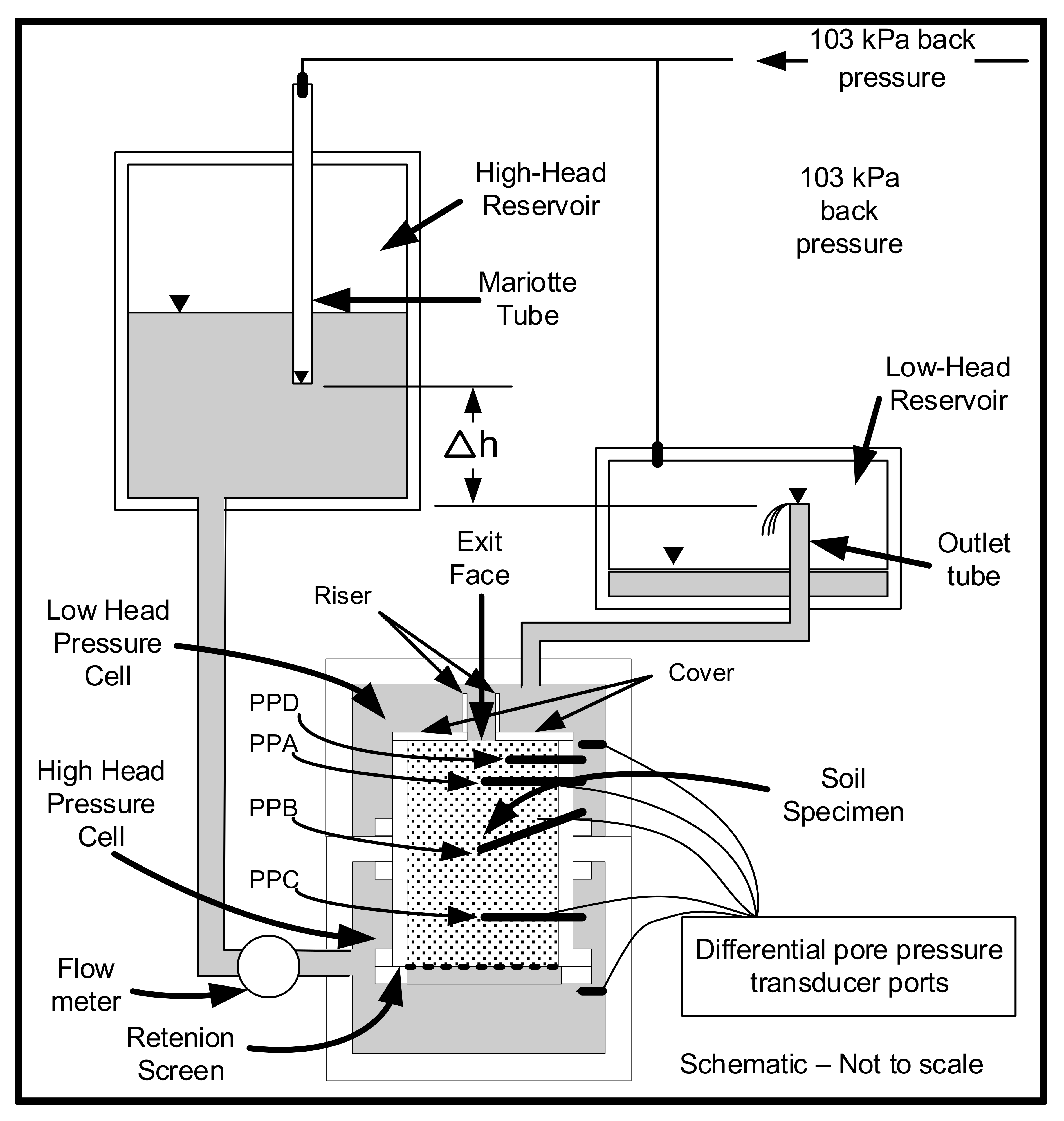
Testing Apparatus. The laboratory models for this study were conducted using the laboratory apparatus used in previous studies at Utah State University [3]. The apparatus imposes an upward seepage on a soil sample to initiate BEP as illustrated in Figure 2.
The soil sample is constricted in a rigid-walled, plexiglass sample holder that is sealed in a vertical position between two pressure cells. With the high-head reservoirs connected to the bottom cell (high-head pressure cell) and low-head reservoirs to the top cell (low-head pressure cell), the differential head across the sample is controlled by raising the Mariotte tube. The system forces flow vertical through the soil specimen (from bottom to top) and exit into a constricted vertical outlet at the top of the sample to model the initiation of BEP through an impermeable clay layer. This system with application of back pressure is to assist in the saturation of the sample and apparatus.
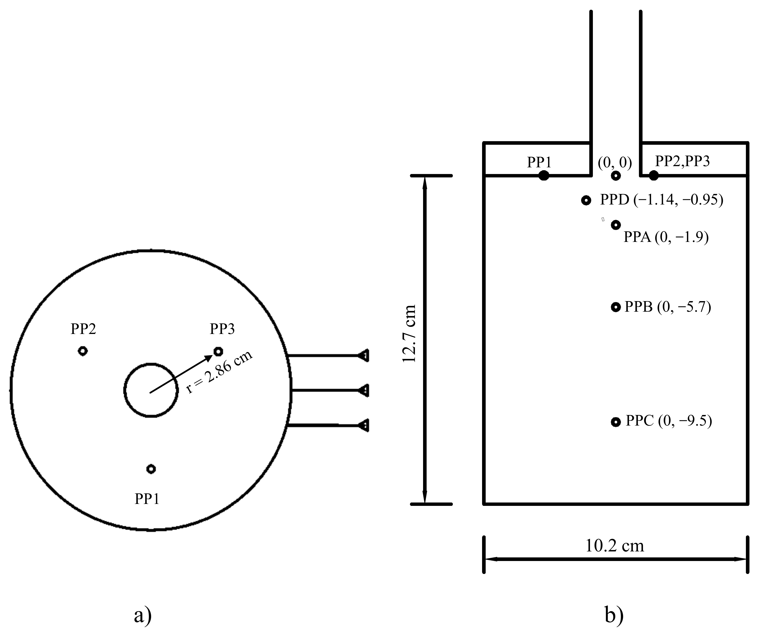
The soil sampler is a 12.7 cm high by 10.2 cm diameter Plexiglas cylinder with a plate sealed over the top to form a constricted exit (see Figure 2). The plate contains a circular orifice (diameters of 1.9 cm in this paper) at the center with a 5.1 cm-high riser tube of the same inside diameter that allows the soil to heave more uniformly. The inside walls of the sample holder are coated with silicone gel that not only provides a frictional interface between the soil and the sample holder, but also prevents the potential for a preferred seepage path to occur along the edges of the sample due to the smooth rigid Plexiglas surface. Two silicone sheets are placed between the soil and the top plate to resemble the contact in field conditions between the soil and clay. Screens have been placed to cover the bottom base for retaining the soil particles while allowing water to flow freely into the soil sample.
Figure 3 shows the locations of seven pore pressure measurement ports located in the soil sample. Four ports are located inside the soil sample: three along the vertical sample axis at distances of 1.9, 5.7 and 9.5 cm below the top and the fourth at a distance of 0.95 cm from the top and shifted 1.14 cm away from the center. The rest of other three ports are located at the top of the soil sample (right underneath the top plate) at a radius of 2.86 cm away from center of the riser, with 120-degree intervals for each.
For all the experiments, the seven pressure transducer ports were connected to Validyne DP15-26 differential pressure transducers to measure the differential hydraulic head between the ports and the low-head reservoir (top of sample). The flow rate was measured with a Kobold magnetic-flux flowmeter between the reservoirs in the tests. Data were collected by a Campbell Scientific CR3000 data logger (Campbell Scientific, Logan, Utah) that was connected to a computer for real-time observation throughout the tests. A video was taken throughout each test and ensured response to each stage of the channel development in more specific detail.
Testing Procedure. The tests were conducted using the following sequence:
- Oven-dried soils were slowly placed in the sample holder and compacted through tapping the outside of the holder with a metal rod in 1.2 cm lifts.
- The two silicone sheets and the riser were sealed on top of the soil sample. The soils were densified by compressing the silicon and riser after a slight overfilling of the cylinder.
- The sample was saturated by: (a) flushing it with carbon dioxide, (b) slowly filling the pressure cells and sample with deaired water from bottom to top, and (c) applying backpressure of 103 kPa.
- Prior to initiating the flow, the video recording and data collection were initiated, and the differential heads for all pore pressure transducers were zeroed to the low-head reservoir.
- The differential head for each test was gradually increased in increments of about 1.2 cm (almost increasing the hydraulic gradient by 0.1) after the first movement of any grain was visually observed. The increments rate was then decreased to about 0.6 cm (almost increasing the hydraulic gradient by 0.05) for the remainder of the test, allowing the sample to observe active BEP and keep the head constant until reaching equilibrium at each stage before further increasing. The test was either finally progressed to complete failure of the sample or reached equilibrium with the maximum differential head of the device.
Soil Tested. Tests were performed on three sandy soils: (1) graded Ottawa sand (well-rounded silica sand) conforming to ASTMC778-03 [26], (2) angular silica sand with identical gradation matching that of the graded Ottawa sand, and (3) uniform, fine-grained (No. 100 sieve) garnet sand, and (4) zirconium-oxide beads with identical gradation matching that of the graded Ottawa sand. Therefore, the test soils vary in shape, gradation and size and that has satisfied the diversity of soils for analysis. A summary of critical properties and characteristics for all four soils tested is provided in Table 1.
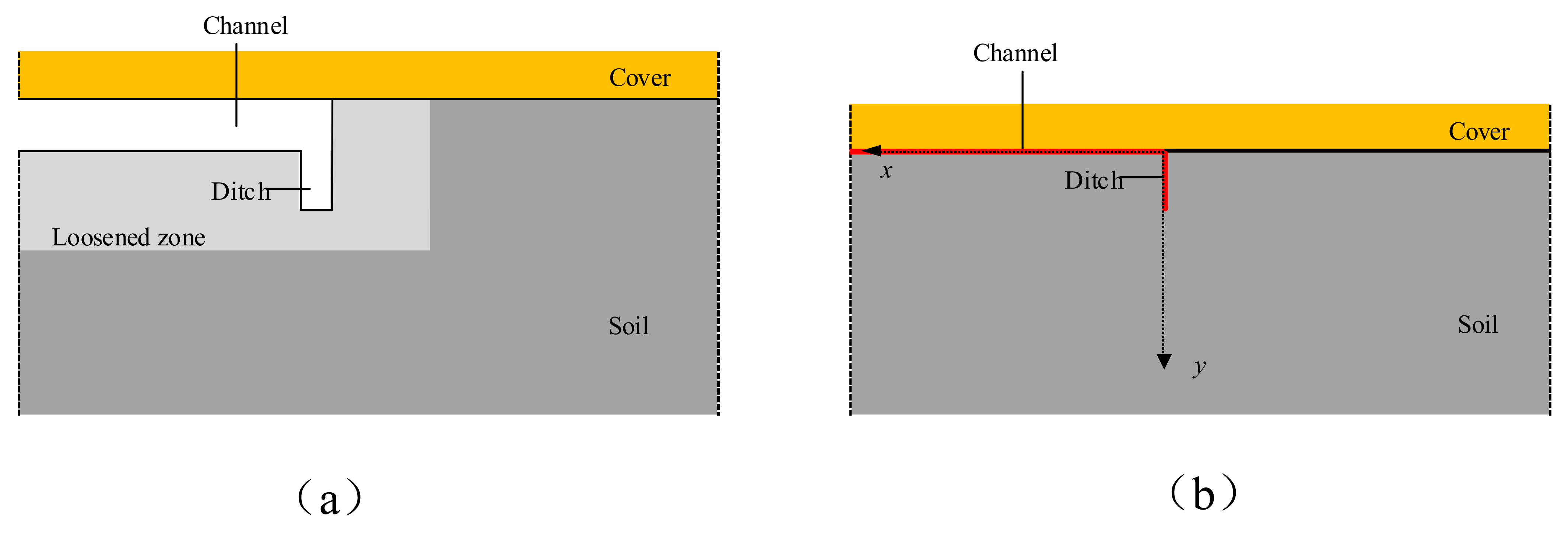
Analytical Model. Most experiments to investigate BEP criteria are performed in flume with a unidirectional flow, however, in backward erosion experiments as well as in field conditions, the flow pattern is not unidirectional [22]. The average gradient (H/L) across the structure is therefore not equal to the local exit gradient (il) near the downstream blanket defect. Numerical models can be refined to predict the gradients close to the singularity, but frequently this will result in an averaged value for the exit gradient rather than an exact value. The numerical model is therefore limited to calculate the local gradient with a certain distance from the front of the channel tip and hardly predicts the actual gradient located very close to the front of the channel tip. The analytical solutions are preferable to numerical models of the channel progression, and the local exit gradient at the vertical section of the channel tip had been successfully assessed by an analytical model as a function of the distance from the channel tip using groundwater calculations for the specific geometry [25], which is revealed through experimental observation by Xiao et al. [27] A shallow ditch appears at the head of the channel before further channel development.
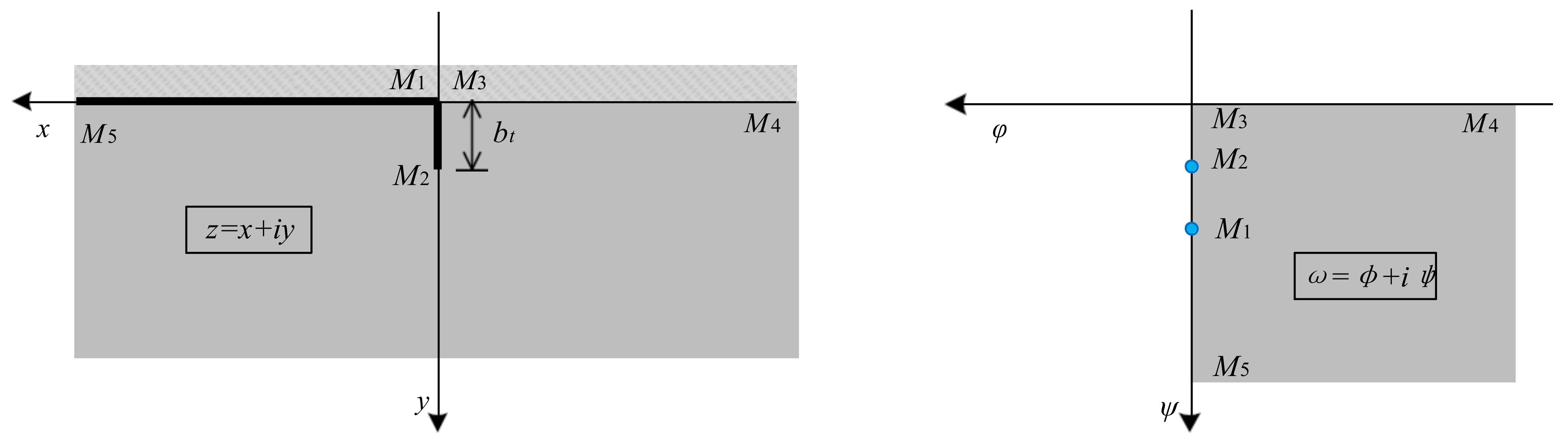
Methodology. [25]. Figure 4a presents the schematic illustration of the channel tip, and the vertical section of the channel tip is simplified for the numerical analysis, as shown in Figure 4b.
The complex potential ω can be proposed using Equation (1):
where Φ is the ground water potential, K the permeability, H the groundwater head, and Ψ the stream function depending on the complex coordinate z (z = x + iy)), which can be obtained from the configuration in Figure 5.
ω = Φ + i Ψ = −KH + i Ψ
The mapping was fulfilled using Equation (2):
where bt is the depth of the ditch and T is a constant number. When the condition meets or and Re(z) < 0, take a minus sign for the Equation (2), otherwise it should be a positive sign.
The complex coordinate z can be obtained as a function of a complex potential ω in Equation (3):
where the selection of positive and negative signs is the same as Equation (2).
When the head (H0) at a point (z = x0 + iy0) outside the ditch in Equation (2) is known, then the constant T can be calculated in Equation (4):
where the selection of positive and negative signs is the same as Equation (2). As any point on the top of the sandy layer in front of the channel tip can be taken into account as yi = 0 and xi < 0 (the head is equal to Hi), then T in Equation (4) can be presented as:
where the selection of positive and negative signs is the same as Equation (2).
3. Results and Discussion
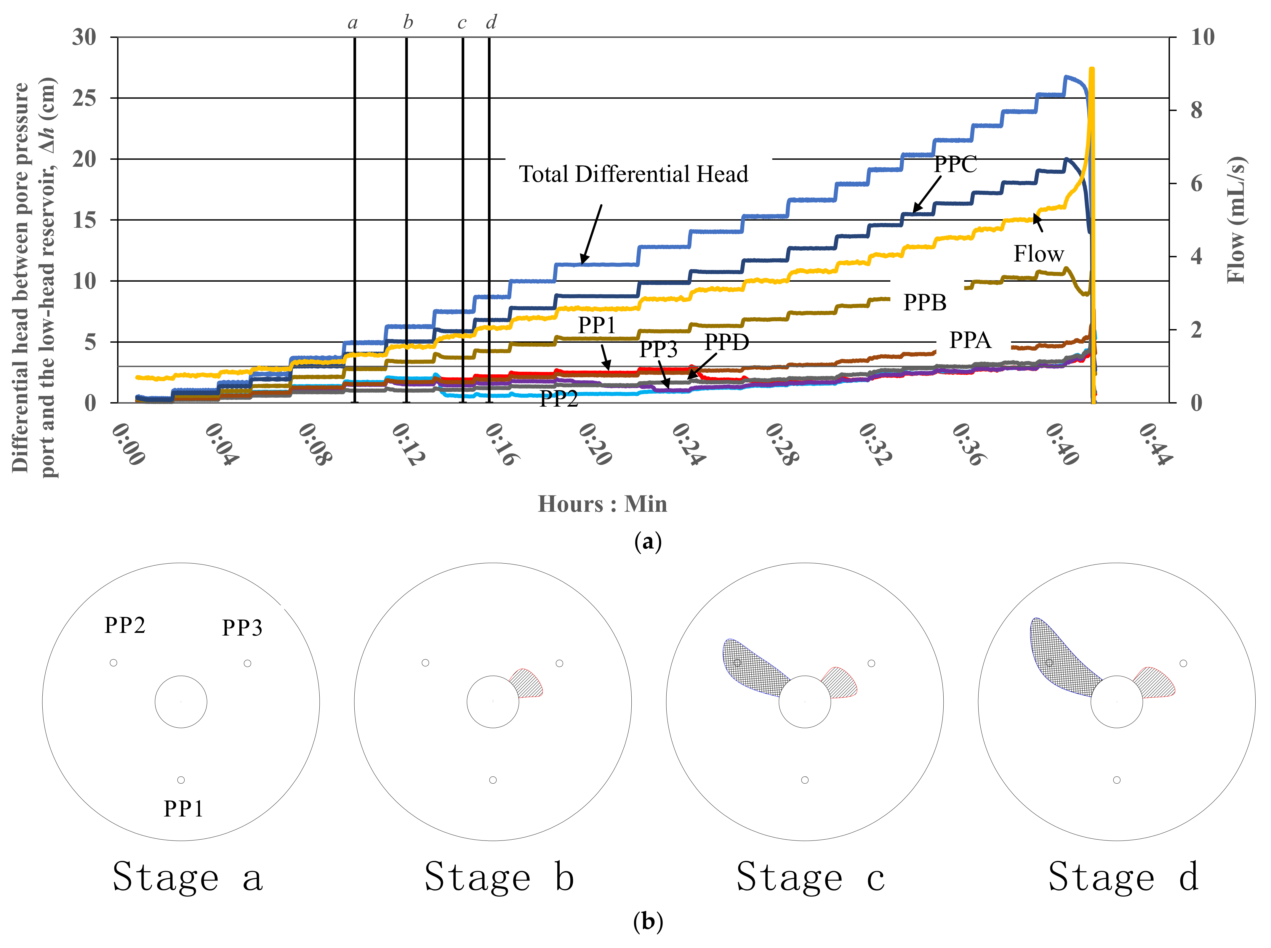
Typical Test Results. Each test provided a time history of the raw data that includes the differential head of each pore pressure port, the total differential head, and the flow. An example test run on graded angular soil along with the associated flow rate can be seen in Figure 6a. Visual observations of progressing erosion were made from the video recorded through the top of the sample top plate. Three observable soil behaviors were identified in the development of BEP erosion in the test apparatus: initial movement, sand boil formation, channel initiation and progression. The first visible movement was observed as a slight heave or rocking movement of individual sand grains along the exit face. This movement was difficult to detect and often required repeated viewing of the portion of the video where movement first occurred. Then one or several sand boils formed on the exit face. The first boil was generally initiated at the edge of the exit face, then additional boils were detected at other locations on the exit face. As the differential head continued to increase, one or several channels initiated at the edge of the exit face and then developed between the riser and the sample at the limited range between the edge of the riser and the edge of the sample holder.
Vertical lines representing key stages (a through d) and sketches of the BEP progression are plotted on Figure 6a,b, respectively. On the basis of observation and recorded data, stage a represents the stage when the BEP had initiated boiling and reached equilibrium prior to channel initiation, and stages b, c and d represent the stages the differential heads for all the sensors responded to channel development. For example, a test where the channel progressed quickly in the direction of PP2 between stages b and c in Figure 6b corresponded with a dramatic drop in the head value of PP2 in Figure 6a, thus illustrating how PP2 deviates from the ambient conditions as a result of the channel formation.
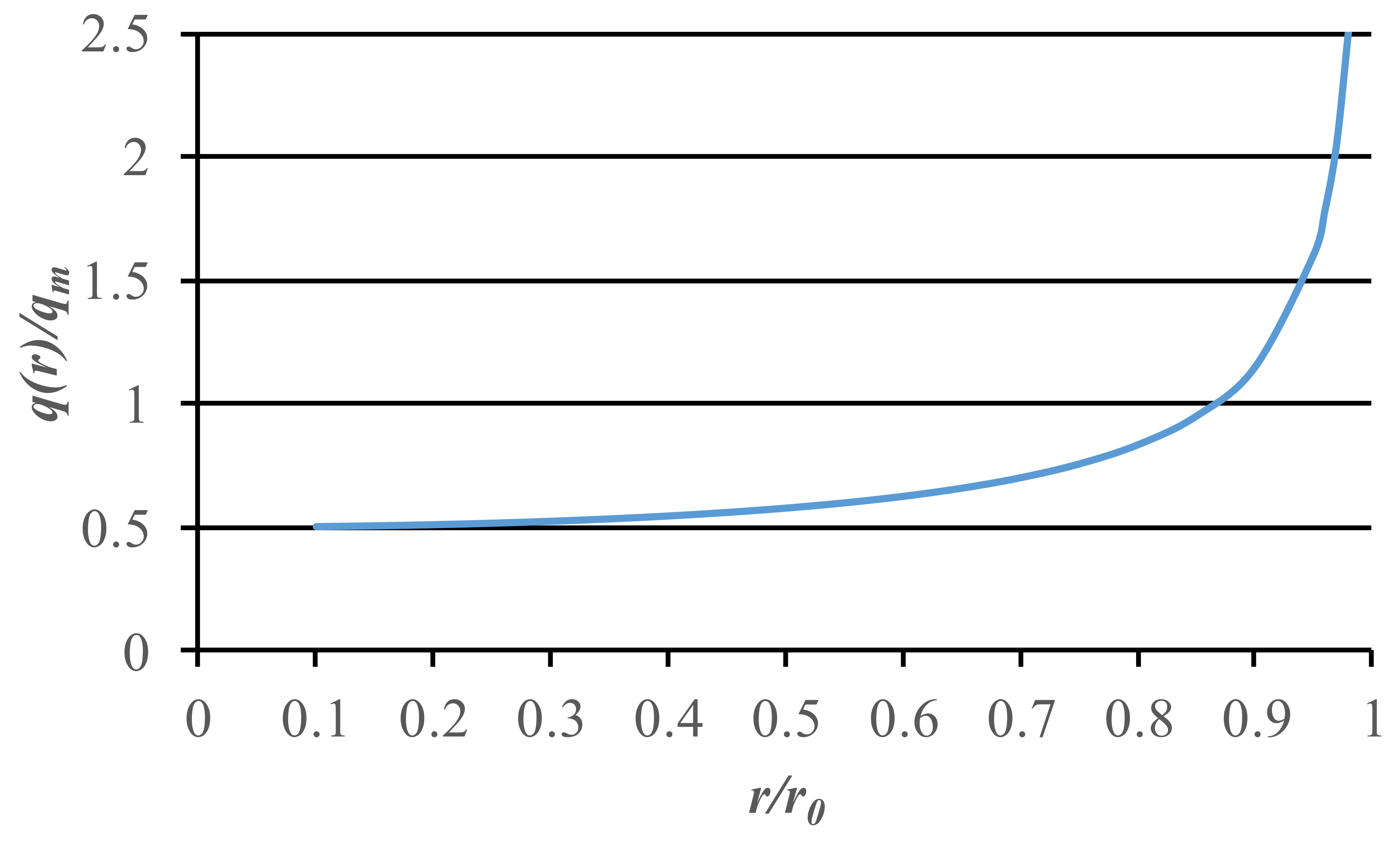
Mechanisms of BEP. First visible movement occurs when the seepage force and the viscous shear forces reach the magnitude of the retaining forces (buoyant weight and intergranular forces) on the soil grains at the exit face. At this point, the surface grains around the edge of the riser are in a state of incipient movement and begin to move with the increasing hydraulic gradient. As the hydraulic gradient across the sample is again increased, the surface grains loosen until a maximum void ratio is achieved. Additional increases in the gradient reduce the downward force of the upper grains on the next layer of underlying grains, thus allowing them to loosen until they have reached a state of equilibrium. This process continues with an increasing gradient across the sample as the loosened zone increases in thickness and sand boils form around the edge of the riser. The position of first visible movement and sand boils can be explained as below using a calculated flow density curve and cumulative flow curve based on Equations (8) and (9) that were originally proposed by Wu [28]. The curves can be seen in Figure 7 and Figure 8, respectively.
where q(r) = flow density at radius r; qm = average flow per unit area at the bottom of shallow wells; H = differential head between the well and the infinite distance from the well; r = the distance from the center of the riser; r0 = radius of the riser.
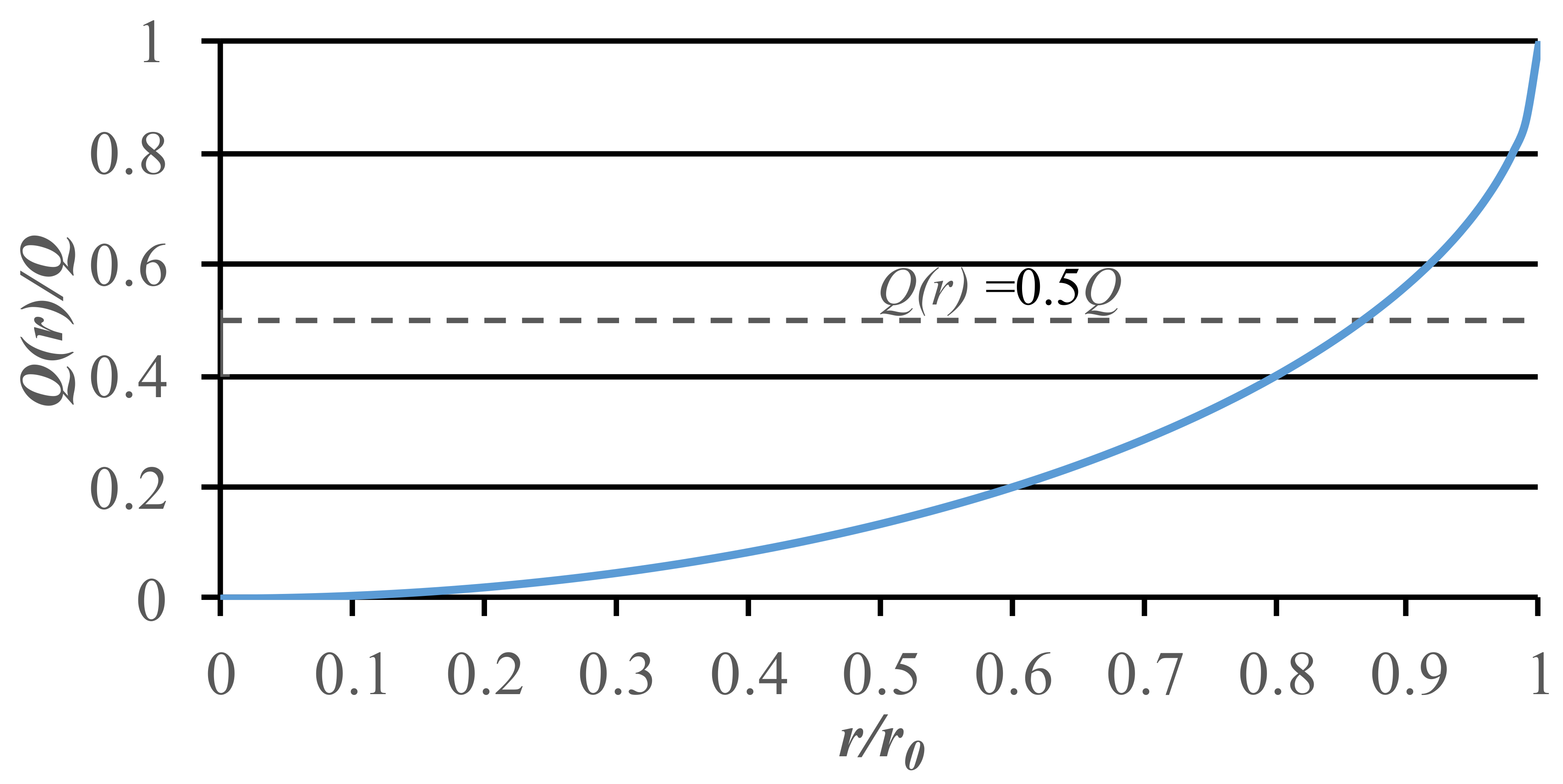
where Q(r) = flow at a radius r; Q = total flow at the bottom of shallow wells; qm = average flow per unit area at the bottom of shallow wells.
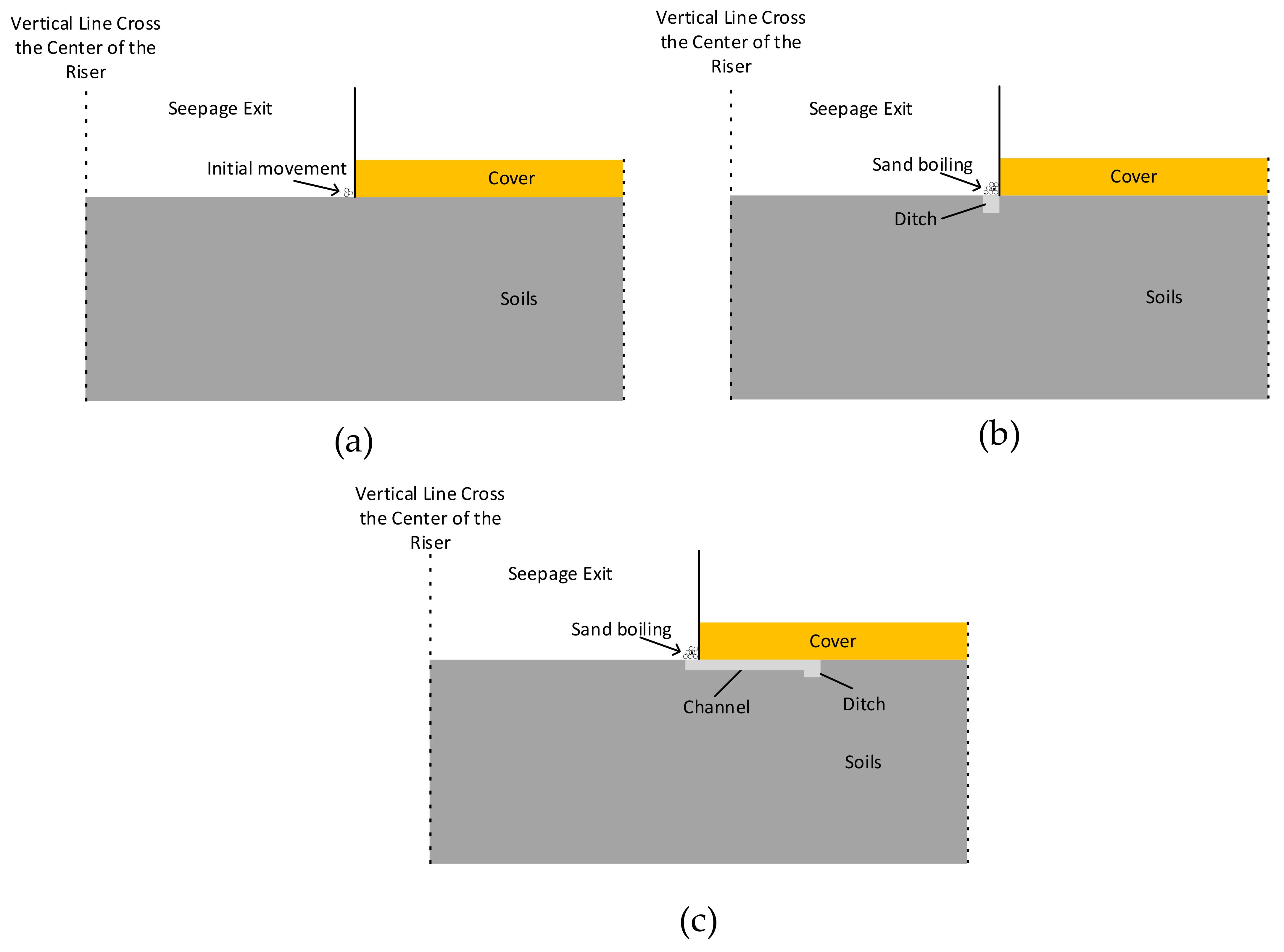
Figure 7 shows that the flow density q(r) is around half of the average flow per unit area at the bottom of shallow wells qm and increases to infinity around the edge of the riser, while Figure 8 shows that over half of the total flow is concentrated at the edge of the riser, which accounts for about a quarter of the total area. Thus, the preferential pathway pressure from increased gradients is concentrated around the edge of the riser. At the same time, the particles in the horizontal direction are subjected to the horizontal seepage force from the surroundings and the frictional force from the cover plate. The particles achieve equilibrium in the horizontal direction but initial movement and progress to sand boiling in the vertical direction appear, as can be seen in Figure 9a.
As the hydraulic gradient further increases, the vertical direction of the narrow ditch increases its size by progressing deeper underneath the edge of the riser, then more particles become loose to maintain vertical equilibrium. As the horizontal seepage force acting on the soil particles, which are located both under the roof of the cover and near to the ditch (as seen in Figure 9b), increases rapidly, the surrounding particles are then allowed to move into the ditch where a BEP channel is formed.
After the channel is formed, then the erosion progression is mainly focused on channel development, as seen in Figure 9c. The assessment of the channel development can be determined by whether the critical value of the soil to maintain the equilibrium located in front of the channel tip is exceeded. With consideration to the vertical force-balance analysis of the soil near the channel tip, the soil will push the cover upward when the vertical seepage force fy acting on the soil is greater than its effective gravity G’, causing the test cell cover to provide counterforce to the soil. However, the upward force acting on the cover is much less than the critical force to cause deformation of the cover, and then the soil in front of the channel reaches a state of vertical equilibrium. As the vertical equilibrium is achieved, further erosion is determined by the horizontal condition. One of the controlled forces is the horizontal force fx from the seepage force acting on the soil, which is determined by the horizontal gradients acting on the tip of the channel and the ditch depth. When the horizontal seepage force intends to push the soil to initiate movement, the frictional force f caused by the contact between the soil strip and the cover plate is initiated. The frictional force can be calculated based on the frictional coefficient of the cover multiplied by its resistance force (fy − G’), which is used to maintain vertical equilibrium. As described above, the erosion propagation will first lead to increasing the ditch depth of the soil in front of the channel tip, then the horizontal force fx is increased when the frictional force f remains constant without further increasing the total differential head across the sample. As the horizontal force continues to grow to exceed the frictional force f, then the soil in front of the channel collapses and falls into the ditch, leading to channel development until equilibrium is achieved or total failure occurs.
Application of analytical model. Experimental data and observations were analyzed, consisting of the following steps for using the numerical analysis. The following discussion uses the graded angular sand test in Figure 6 as an example to provide details on the application, with four steps outlined for back-calculation of the head of sensor PP3.
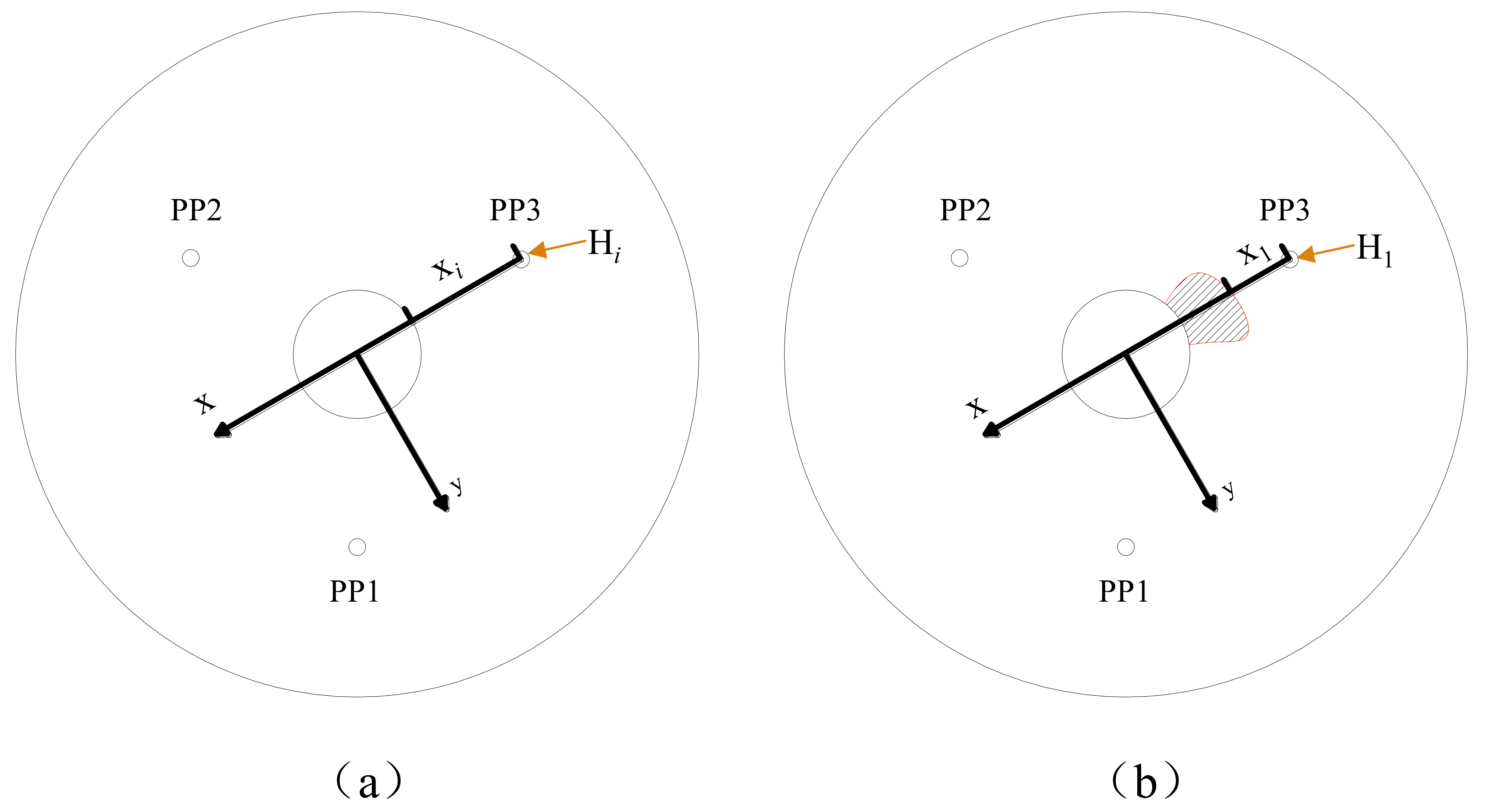
Step 1. The last stage prior to channel initiation (Stage a), an initial head of the sensor PP3, Hi, represents the point that the differential pressure head of the sensor was increased from zero (see Figure 10a). Then, a channel was initiated in front of the sensor and developed between the sensor and the circular exit (see Figure 10b).
Step 2. As the sensor PP3 was located on the x-axis (as seen in Figure 10a) its y-axis coordinate is zero. Therefore, the distance between the sensor PP3 and the edge of the circular exit, xi, prior to channel initiation was measured to represent its x-axis coordinate. It should be noted the distance was measured on the top of sample and contrary to the x-direction, thus yi = 0 and xi < 0. By knowing that the depth of the channel is zero (bti = 0) before initiation, the point with known head Hi, coordinates (xi, yi = 0), and the depth of the channel (bti = 0) can be input into Equation (5) resulting in Equation (6) for the constant T:
Step 3. At a later stage (Stage b), a piping channel was initiated and developed in the physical model around the orifice, and the observed distance between the sensor and the assumed channel tip could be measured. As described above, the simplified numerical solution was conducted using two-dimensional analysis. The assumed channel tip is located at the line which is between the sensor and the center of the circular exit, instead of the tip of the horizontal channel shape based on direct observations from the video. Thus, the distance between the sensor and the assumed channel tip was measured as x1, and y1 = 0 (see Figure 10b). The channels are assumed with a depth of 2.5 times the average grain size (bt1 = 0.075 cm) based on measurement of channel depths in small-scale backward erosion piping experiments by others [7,27,29]. Through substitution of calculated constant T from Equation (6), coordinates of (x1, y1) and the depth of the channel (bt1 = 0.075 cm) into Equation (5), the head of the sensor PP3, H1, can be calculated by Equation (7):
Step 4. As the total differential head was increased, the channel was again developed. When the assumed channel tip in front of the sensor propagated, the distance between the sensor and the assumed channel tip was again measured as x2, and y2 = 0 for Stage c and x3, and y3 = 0 for Stage d, and the procedure of Step 3 was repeated to back-calculate the head of sensor PP3 as H2 and H3, respectively. As the channel was further developed, the distance from the sensor was less than 30 times the average grain size, and the repetition was seized. This is because the effect of any loosened zone significantly enlarged surrounding the channel tip, based on the measurements from others [27]. Therefore, the head of the sensor was significantly deviated when the distance between the assumed channel tip and the sensor reached a critical state, then causing the deviation between numerical results and the experimental ones. In addition, it is also important to acknowledge factors that may exist in the physical models that are not considered in the analytical assumptions, such as multiple channels having an impact on each other, friction between the riser and the soil caused by the silicon sheet, and the fact that the sample compaction is not entirely uniform during the process of the channel development.
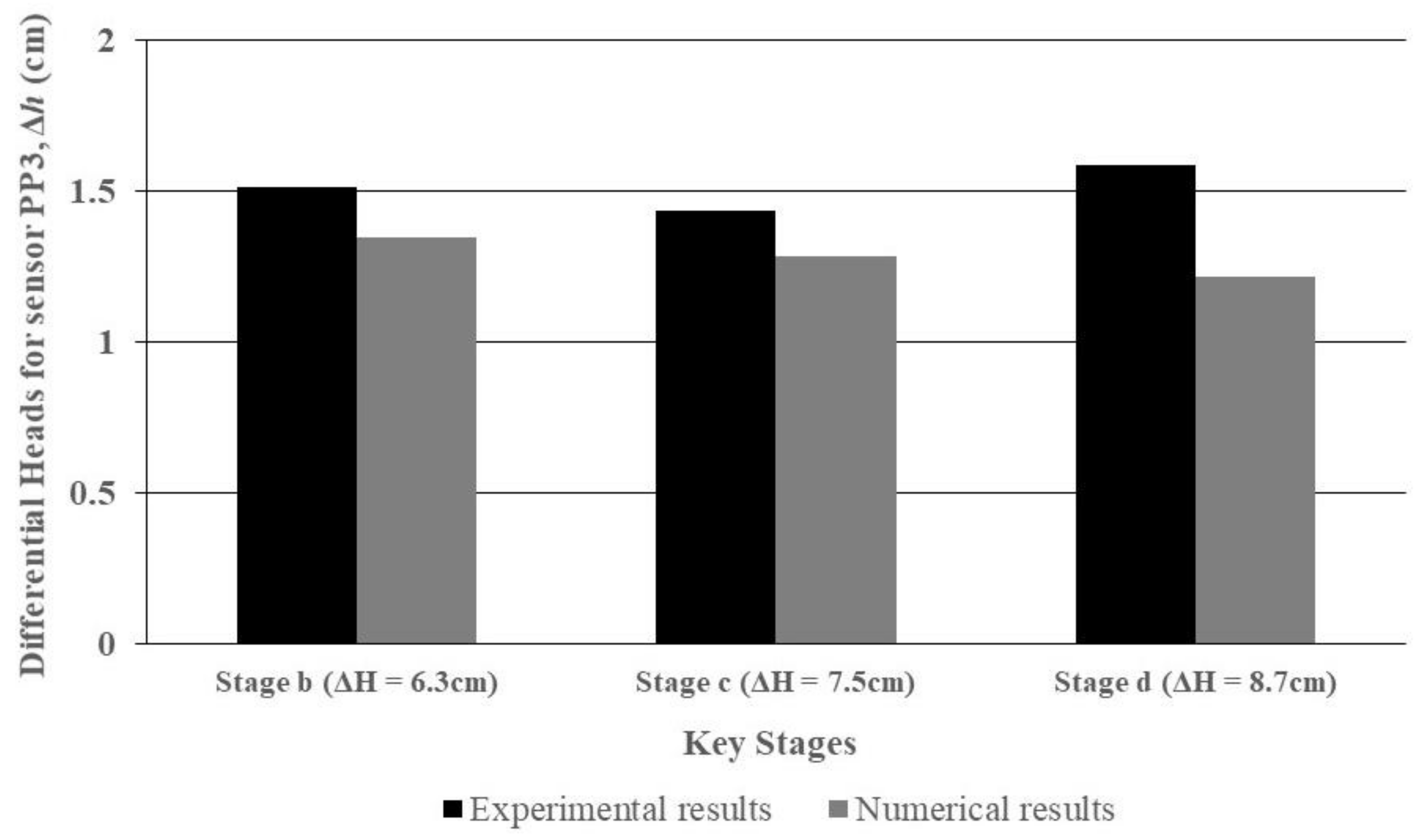
Comparisons were made to assess how well the analytical model result correlated with actual measured values. Figure 11 presents a comparison of experimental and measured results of three key stages (stages with a total differential head of 6.3, 7.5 and 8.7 cm, see Figure 6b) for sensor PP3 on graded angular sand. As the channels were further developed, the differential head of the sensor PP3 decreased, as well the calculated head of using the model decreased. Theoretically, the differential head of a sensor decreases dramatically when a channel is formed in front or nearby, but the surrounding loosened zone occupies a proportional seepage concentration that will slow down the sensor’s reaction regarding decreasing its differential head. However, it is important to acknowledge the loosened zone that exists in the physical models that is not considered in the analytical assumptions, as the effect of any loosened zone significantly enlarged surrounding the channel tip, based on the measurements from others [27].
Greater variations occurred in the later test stages, and these are because differential loosening has occurred without being observable, which is formed in front of or below the channel when the channel progresses to reach closer to the sensor, such as in the example test in Figure 6 when the erosion was developed after stage d. The maximum deviation generally came from the influence of other channels that simultaneously formed in same experiment, which changed the hydraulic conditions around the exit to cause the deflection of the sensor’s reaction to channel development. For example, the measured result for one of the sensors was most likely affected by the channel progression that was occurring in front of or near to the surroundings when several other channels were also developing in the early stages during the erosion process of the entire test. Moreover, a portion of the observed error can also be attributed to the distance while the channel tip is approaching the sensor. Although the results of numerical model present lower values than the experimental results due to these reasons, it can be seen that the deviations among all the stages were still being controlled in a very small range between the experimental and numerical results.
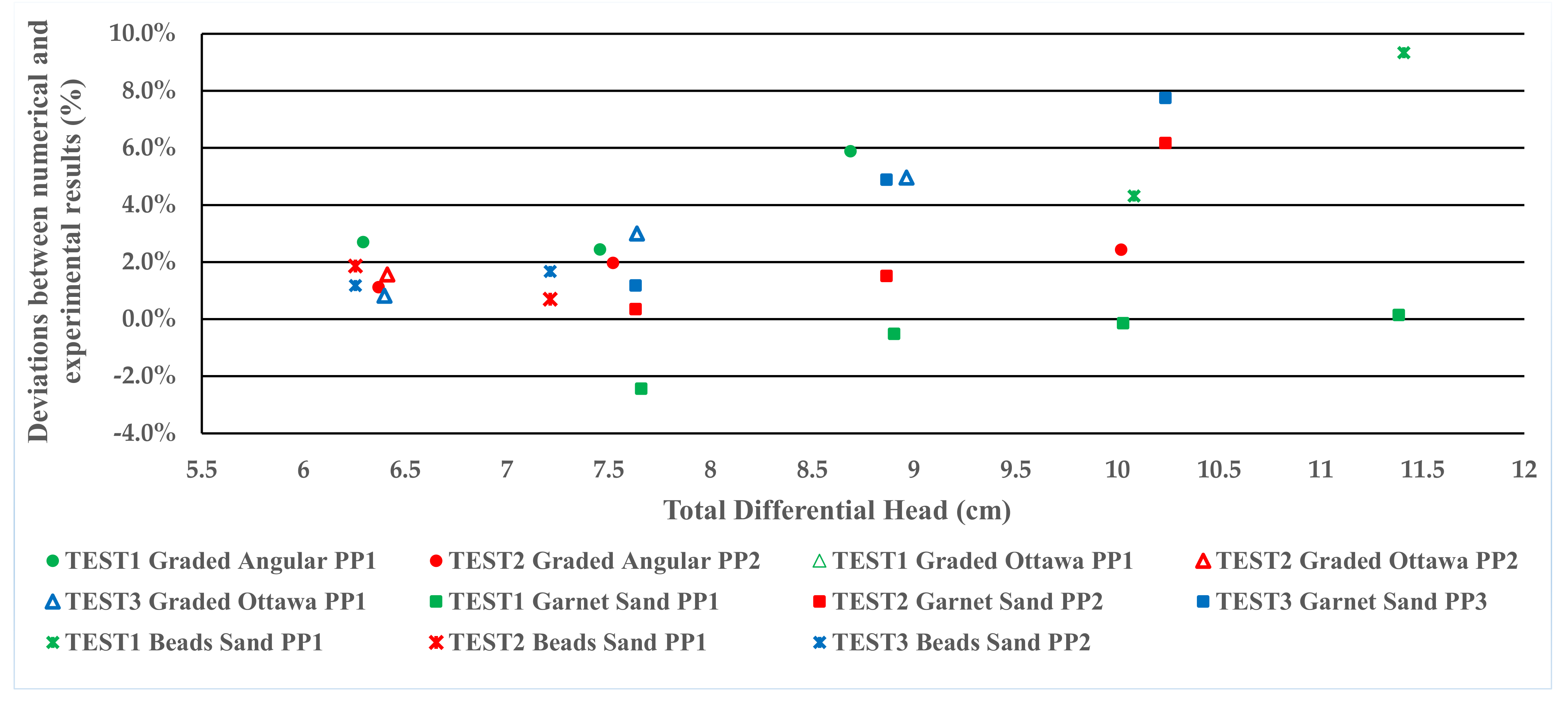
As three repeated tests for each soil had been conducted without any property change, the numerical model was applied to 11 tests for four different soils. The exception was the third test for graded angular sand because multiple channels initiated at the same period, then the changes of differential head for the sensors interfered with both channels to cause additional deviations, and it was obviously not possible to apply the model for the back-calculation. Figure 12 presents a summary of comparison results from plots, similar to Figure 11, for all the soils, and the laboratory results were compared to numerical results. The differential estimation for each stage was based on the difference between measured pore pressures and numerical results versus the total differential head of the stage. As seen from Figure 12, only one sensor from each test was taken into account for comparison, and the reason was necessarily discussed as follows. As the channel was initiated in a random direction around the riser, the applied sensor in each test for comparison varies by the real condition. For example, the first channel was initiated near to or in front of the sensor PP1, then the model was applied to back-calculate the differential heads of this sensor instead of the other two. This is because the hydraulic condition between the sensor (PP2/PP3) and the riser is more likely in the ambient condition, for which the pore pressure regime exists prior to any changes in the soil structure between them. As the total of differential heads was increased, the channel was then further developed and the differential head of the sensor PP1 decreased proportionally with the distance to the channel tip. In the same period, as seepage concentrated between the sensor and channel, which decreased the seepage portion between PP2/PP3 to the edge of the riser. It can also be recognized that the soil structure between sensor PP2/PP3 and the edge of the riser is still within the ambient condition, but the differential head of the sensor had deviated the ambient condition as the seepage portions increased lower than expected. As observed from the test, the channel was not initiated between sensor PP2/PP3 and the edge of the riser at this stage. Therefore, the analytical model should be applied to back-calculate the head of either of the two sensors, while the deviations were initiated, but the channel development between the sensors and the riser was not responsible for these early deviations. This means the model found it difficult to calculate the heads of these two sensors preciously after the first channel had initiated and developed in the direction between sensor PP1 and the edge of the riser. It should also be noted that only the three sensors as in one plane at the top of the sample had been used for this analysis. This is because the other four sensors located vertically inside the sample are used to measure the critical gradients for soil loosening and the mechanism to create or expand the loosened zone, which is the very first stage of initiation of the erosion. Therefore, the analytical model is validated for its capability of predicting the progress of channel development, the erosion of which develops in a horizontal direction instead of the vertical progression of the soil loosening.
As discussed above, the deviations between experimental and numerical results are increased within the channel development, which is validated in Figure 12. The deviation of most tests is less than 4% and the maximum deviation of these tests is no more than 10% for all the test stages. As seen in the aforementioned figure, some tests with more rounded soil appeared to be detected at relatively higher deviations than the others. The authors surmise that it is more attributable to the effect of soil loosening, which causes such deviations when the erosion is propagated in the later stages. However, as seen in the figure, the results between the numerical and experimental data stayed in very close agreement for the different soils when the shape, gradation and size of the soils varied.
4. Conclusions
The initiation and progression of backward erosion piping around the exit area in uniformly graded sands was assessed through laboratory tests. The observations and pore pressure measurements were interpreted by rectifying the observed progression and changes in the flow regime using an analytical model. The analytical model for predicting BEP initiation progression on the basis of the effect of a ditch in front of a channel tip was found to provide accurately calculated results, corresponding with the general observed and measured conditions at various stages of BEP development.
The mechanisms of BEP initiation and early progression in sandy soils when a defect was present in an overlying soil blanket were studied. The position of the first visible movement and sand boils were assessed as the preferential pathway pressure from increased gradients which are concentrated around the edge of the riser. The soil particles in front of the channel tip can achieve equilibrium with the cover providing counterforce to the soil, and the channel will progress backward to seepage force only due to a horizontal seepage force greater than the frictional force acting on soils caused by the contact with the cover plate.
The model has only evaluated the validity of the application on small-scale experiments. Further research is needed to provide more insights into the mechanisms of BEP and the capability to predict the occurrence of BEP over a range of problem scales.
Author Contributions
S.P. wrote the main manuscript text and prepared all the figures and tables. S.P. and J.D.R. contributed to the experiments. H.P., S.P., H.C. and G.L. developed the methodology. All authors have read and agreed to the published version of the manuscript.
Funding
This research was funded by National Natural Science Foundation of China (Grant No. 51978282), the Natural Science Foundation of Guangdong Province (2020A1515010583) State Key Lab of Subtropical Building Science, South China University of Technology (2022ZB21) and Guangdong Provincial Key Laboratory of Modern Civil Engineering Technology (2021B1212040003). And The APC was funded by State Key Lab of Subtropical Building Science, South China University of Technology (2022ZB21).
Data Availability Statement
The datasets used and/or analyzed during the current study are available from the corresponding author on reasonable request.
Acknowledgments
The authors would like to acknowledge the support of National Natural Science Foundation of China (Grant No. 51978282), the Natural Science Foundation of Guangdong Province (2020A1515010583) State Key Lab of Subtropical Building Science, South China University of Technology (2022ZB21) and Guangdong Provincial Key Laboratory of Modern Civil Engineering Technology (2021B1212040003).
Conflicts of Interest
The authors declare that there are no known conflicts of interest associated with this publication and there has been no significant financial support for this work that could have influenced its outcome.
References
- Foster, M.; Fell, R.; Spannagle, M. The statistics of embankment dam failures and accidents. Can. Geotech. J. 2000, 37, 1000–1024. [Google Scholar] [CrossRef]
- Vrijling, J.K.; Kok, M.; Calle, E.O.F.; Epema, W.G.; Van der Meer, M.T.; Van den Berg, P.; Schweckendiek, T. Piping—Realiteit of Rekenfout? Technical Report; Dutch Expertise Network on Flood Protection (ENW): Utrecht, the Netherlands, 2010. (In Dutch) [Google Scholar]
- Peng, S.; Rice, J. Inverse analysis of laboratory data and observations for evaluation of backward erosion piping process. J. Rock Mech. Geotech. Eng. 2020, 12, 1080–1092. [Google Scholar] [CrossRef]
- Fleshman, M.; Rice, J. Laboratory modeling of the mechanisms of piping erosion initiation. J. Geotech. Geoenviron. Eng. 2014, 140, 04014017. [Google Scholar] [CrossRef]
- Allan, R.J. Backward Erosion Piping. Ph.D. Thesis, University of New South Wales, Sydney, Australia, 2018. [Google Scholar]
- Van Beek, V.M.; Bezuijen, A.; Sellmeijer, H. Backward Erosion Piping. In Erosion in Geomechanics Applied to Dams and Levees; Bonelli, S., Ed.; Wiley: London, UK; Hoboken, NJ, USA, 2013; pp. 193–269. [Google Scholar]
- Van Beek, V.M. Backward Erosion Piping. Initiation and Progression. Ph.D. Thesis, Technische Universiteit Delft, Delft, The Netherlands, 2015. [Google Scholar]
- De Wit, G.N.; Sellmeijer, J.B.; Penning, A. Laboratory tests on piping. In Proceeding of 10th International Conference Soil Mechanics and Foundation Engineering, Stockholm, Sweden, 15–19 June 1981; pp. 517–520. [Google Scholar]
- Sellmeijer, J.B. On the Mechanism of Piping under Impervious Structures. Doctoral Dissertation, Technische Universiteit Delft, Delft, The Netherlands, 1988. [Google Scholar]
- Koenders, M.A.; Sellmeijer, J.B. Mathematical model for piping. J. Geotech. Eng. 1992, 118, 943–946. [Google Scholar] [CrossRef]
- Weijers, J.B.A.; Sellmeijer, J.B.A. A new model to deal with the piping mechanism on filters, in geotechnical and hydraulic engineering. In Filters in Geotechnical and Hydrauilc Engineering; Brauns, J., Herbaum, M., Schuler, U., Eds.; Balkema: Rotterdam, The Netherlands, 1993; pp. 349–355. [Google Scholar]
- Miesel, D. Rückschreitende Erosion unter Bindiger Deckschicht. Baugrundtagung; Deutschen Gesellschaft für Erd- und Grundbau e.V.: Essen, Germany, 1978; pp. 599–626. (In German) [Google Scholar]
- Hanses, U. Zur Mechanik der Entwicklung von Erosionskanälen in Geschichtetem Untergrund unter Stauanlagen. Master’s Thesis, Grundbauinstitut der Technischen Universität Berlin, Berlin, Germany, 1985. (In German). [Google Scholar]
- Müller-Kirchenbauer, H.; Rankl, M.; Schlötzer, C. Mechanism for regressive erosion beneath dams and barrages. In Filters in Geotechnical and Hydraulic Engineering; Balkema: Rotterdam, The Netherlands, 1993; pp. 369–376. [Google Scholar]
- De Wit, J.M. Onderzoek Zandmeevoerende Wellen Rapportage Modelproeven. Rep. No. CO-220885/10; Grondmechanica Delft: Delft, Netherlands, 1984. [Google Scholar]
- Pietrus, T.J. An experimental Investigation of Hydraulic Piping in Sand. Master Dissertation, University of Florida, Gainesville, FL, USA, 1981. [Google Scholar]
- Townsend, F.C.D.; Bloomquist, D.; Shiau, J.M.; Martinez, R.; Rubin, H. Evaluation of Filter Criteria and Thickness for Mitigating Piping in Sand; University of Florida: Gainesville, FL, USA, 1988. [Google Scholar]
- Van Beek, V.M.; van Knoeff, J.G.; Sellmeijer, J.B. Observations on the process of backward piping by underseepage in cohesionless soils in small-, medium- and full-scale experiments. Eur. J. Environ. Civ. Eng. 2011, 15, 1115–1137. [Google Scholar]
- Schmertmann, J.H. The Non-Filter Factor of Safety against Piping through Sand. ASCE Geotechnical Special Publication No. 111, Judgment and Innovation; Silva, F., Kavazanjian, E., Eds.; ASCE: Reston, VA, USA, 2000; pp. 65–132. [Google Scholar]
- Sellmeijer, J.B.; de la Cruz, J.L.; van Beek, V.M.; Knoeff, H. Fine-tuning of the piping model through smallscale, medium-scale and IJkdijk experiments. Eur. J. Environ. Civ. Eng. 2011, 15, 1139–1154. [Google Scholar] [CrossRef]
- Hoffmans, G.; Van Rijn, L. Hydraulic approach for predicting piping in dikes. J. Hydraul. Res. 2018, 56, 268–281. [Google Scholar] [CrossRef]
- Van Beek, V.M.; Bezuijen, A.; Sellmeijer, J.B.; Barends, F.B.J. Initiation of backward erosion piping in uniform sands. Géotechnique 2014, 64, 927–941. [Google Scholar] [CrossRef] [Green Version]
- DeHaan, H.; Stamper, J.; Walters, B. Mississippi River and Tributaries System 2011 Post-Flood Report; USACE: Vicksburg, MS, USA, 2012. [Google Scholar]
- Schaefer, J.A.; O’Leary, T.M.; Robbins, B.A. Assessing the implications of sand boils for backward erosion piping risk. In Geo-Risk 2017: Geotechnical Risk Assessment and Management—GSP 285; ASCE: Reston, VA, USA, 2017. [Google Scholar]
- Xiao, Y.; Cao, H.; Luo, G.; Zhai, C. Modelling seepage flow near the pipe tip. Acta Geotech. 2020, 15, 1953–1966. [Google Scholar] [CrossRef]
- ASTM. Standard Specification for Standard Sand. In Annual Book of ASTM Standards 2003; ASTM International: West Conshohocken, PA, USA, 2003. [Google Scholar]
- Xiao, Y.; Cao, H.; Luo, G. Experimental investigation of the backward erosion mechanism near the pipe tip. Acta Geotech. 2019, 14, 767–781. [Google Scholar] [CrossRef]
- Wu, S. Theory of Seepage Flow for Calculating Layerd Media and Relief Ditches and Relief Wells; Water Resources Press, Anhui Water Resources Research Institute: Beijing, China, 1980; pp. 331–334. (In Chinese) [Google Scholar]
- Vandenboer, K.; van Beek, V.M.; Bezuijen, A. Analysis of the pipe depth development in small-scale backward erosion piping experiments. Acta Geotech. 2019, 14, 477–486. [Google Scholar] [CrossRef]
Figure 1.
Schematic illustration of BEP and the mechanisms of BEP development (Adapted from Peng et al. [3]).
Figure 1.
Schematic illustration of BEP and the mechanisms of BEP development (Adapted from Peng et al. [3]).

Figure 2.
Schematic illustration of the testing apparatus (Adapted from Peng et al. [3]).
Figure 2.
Schematic illustration of the testing apparatus (Adapted from Peng et al. [3]).

Figure 3.
Locations of pore pressure ports within the sample holder: (a) Top view and (b) Side view.
Figure 3.
Locations of pore pressure ports within the sample holder: (a) Top view and (b) Side view.

Figure 4.
Schematic illustration of: (a) the vertical section; (b) the simplified vertical section of the channel tip [25].
Figure 4.
Schematic illustration of: (a) the vertical section; (b) the simplified vertical section of the channel tip [25].

Figure 5.
Conformal mapping schemes for the channel tip [25].
Figure 5.
Conformal mapping schemes for the channel tip [25].

Figure 6.
Test data for graded angular sand: (a) pore pressure and flow data plotted versus time; (b) sketches of BEP development from the video at key stages.
Figure 6.
Test data for graded angular sand: (a) pore pressure and flow data plotted versus time; (b) sketches of BEP development from the video at key stages.

Figure 7.
Flow distribution curve through the exit.

Figure 8.
Cumulative flow curve through the exit.

Figure 9.
Schematic illustration of erosion development of BEP: (a) initial movement; (b) sand boiling; and (c) channel development (the location of the figure being referred to is at the very top of the sample with riser and cover, see Figure 2).
Figure 9.
Schematic illustration of erosion development of BEP: (a) initial movement; (b) sand boiling; and (c) channel development (the location of the figure being referred to is at the very top of the sample with riser and cover, see Figure 2).

Figure 10.
Schematic illustration of BEP development at two key stages of a test on graded angular sand: (a) before channel initiation (Stage a); (b) after channel initiation (Stage b) (stage letters correlate with Figure 6b).
Figure 10.
Schematic illustration of BEP development at two key stages of a test on graded angular sand: (a) before channel initiation (Stage a); (b) after channel initiation (Stage b) (stage letters correlate with Figure 6b).

Figure 11.
Plot comparing measured pore pressures versus numerical results for sensor PP3 in three key stages for graded angular sand.
Figure 11.
Plot comparing measured pore pressures versus numerical results for sensor PP3 in three key stages for graded angular sand.

Figure 12.
Variations between laboratory testing and numerical analysis for the four different types of sands. (Test 1 graded angular PP1 represents the sensor PP1 in the first test of graded angular sand which was applied for comparison).
Figure 12.
Variations between laboratory testing and numerical analysis for the four different types of sands. (Test 1 graded angular PP1 represents the sensor PP1 in the first test of graded angular sand which was applied for comparison).


Table 1.
Properties and characteristics of soils tested.
| Soil Type | GSa | D50b (/mm) | Cuc | Φid (/°) | emin − emax e | ρsat f (kg/m3) | E g | Ψh | ∆ i |
|---|---|---|---|---|---|---|---|---|---|
| Graded Ottawa | 2.65 | 0.37 | 1.76 | 38 | 0.48–0.72 | 2.08 × 10³ | 0.53 | 0.5 | 0.5 |
| Graded Angular | 2.63 | 0.30 | 2.18 | 44 | 0.63–1.15 | 1.89 × 10³ | 0.73 | 0.7 | 0.4 |
| Garnet Sand | 4.05 | 0.15 | 1.25 | 44 | 0.96–1.54 | 2.47 × 10³ | 1.08 | 1.1 | 1.1 |
| Graded Zirconium Beads | 3.84 | 0.37 | 1.57 | 24 | 0.46–0.60 | 2.87 × 10³ | 0.52 | 0.9 | 0.9 |
Notes: a Specific gravity, b Cumulative particle size grain size, c Coefficient of uniformity, d Internal angle of repose, e Min to max void ratio, f Saturated unit mass, g Void ratio, h Sphericity, i Roundness.
Publisher’s Note: MDPI stays neutral with regard to jurisdictional claims in published maps and institutional affiliations. |
© 2022 by the authors. Licensee MDPI, Basel, Switzerland. This article is an open access article distributed under the terms and conditions of the Creative Commons Attribution (CC BY) license (https://creativecommons.org/licenses/by/4.0/).
Share and Cite
MDPI and ACS Style
Pan, H.; Rice, J.D.; Peng, S.; Cao, H.; Luo, G. Analytical Modeling with Laboratory Data and Observations of the Mechanisms of Backward Erosion Piping Development. Water 2022, 14, 3420. https://doi.org/10.3390/w14213420
AMA Style
Pan H, Rice JD, Peng S, Cao H, Luo G. Analytical Modeling with Laboratory Data and Observations of the Mechanisms of Backward Erosion Piping Development. Water. 2022; 14(21):3420. https://doi.org/10.3390/w14213420
Chicago/Turabian StylePan, Hong, John D. Rice, Sige Peng, Hong Cao, and Guanyong Luo. 2022. "Analytical Modeling with Laboratory Data and Observations of the Mechanisms of Backward Erosion Piping Development" Water 14, no. 21: 3420. https://doi.org/10.3390/w14213420
Note that from the first issue of 2016, this journal uses article numbers instead of page numbers. See further details here.