
Assessment of a Multi-Layer Aquifer Vulnerability Using a Multi-Parameter Decision-Making Method in Mosha Plain, Iran


1
Department of Minerals and Groundwater Resources, Faculty of Earth Sciences, Shahid Beheshti University, Tehran 1983969411, Iran
2
Department of Earth Sciences, Utrecht University, 3584 CB Utrecht, The Netherlands
3
Department of Geology, Shahid Bahonar University, Kerman 7619613439, Iran
*
Author to whom correspondence should be addressed.
Water 2022, 14(21), 3397; https://doi.org/10.3390/w14213397
Submission received: 24 September 2022
/
Revised: 12 October 2022
/
Accepted: 21 October 2022
/
Published: 26 October 2022
(This article belongs to the Special Issue Water Quality and Contaminant Transport in Aquatic Environments)
Abstract
:In recent decades, there has been a growing emphasis on assessing aquifer vulnerability. Given the availability of spatial data and the GIS advantages, mapping the groundwater vulnerability has become a common tool for protecting and managing groundwater resources. Here, we applied the GIS indexing and an overlay method to explore a combination of the potential contamination factors needed to assess groundwater vulnerability in the Mosha aquifer. The data from a borehole data logger and chemical analysis of spring water show groundwater responses to the surface contaminating sources. To assess the aquifer vulnerability, the potential contaminating sources were classified into three groups, namely (1) geological characteristics such as lithology and structural geology features; (2) the infrastructures induced by human activities such as roads, water wells, and pit latrines; and (3) land use. By considering these components, the risk maps were produced. Our findings indicate that the aquifer is very responsive to the anthropogenic contaminants that may leak into the aquifer from urbanized areas. Additionally, roads and pit latrines can significantly release pollutants into the environment that may eventually leak into the aquifer and contaminate the underlying groundwater resources.
1. Introduction
Groundwater is considered a valuable and finite natural resource that is the basis for the development of societies. Additionally, groundwaters are the main freshwater resource in semi-arid regions and are usually subjected to anthropogenic contamination such as industrialization, urbanization and agriculture, and inappropriate land use practices [1,2,3,4,5,6]. Progressive aquifer contamination may lead to permanent or temporary loss of water resources, as it may significantly increase the cost of water treatment and remediation [7,8,9]. The concept of groundwater vulnerability is a principal factor in the groundwater contamination evaluation that plays a key role in the actions concerning water resource management [10,11]. An assessment of groundwater contamination may result in maps that divide a specific geographical region into several zones based on their susceptibility to contaminants [12,13,14]. In general, vulnerability includes two types: (1) intrinsic vulnerability that is naturally controlled by the hydrogeological and geological properties of the aquifer, and (2) anthropogenic vulnerability that is caused by the adverse effects of human activities on the aquifer.
Regarding the available data and the characteristics of the aquifer, researchers have developed different methods to identify groundwater vulnerability [15]. These methods can be classified into three major groups, namely (1) statistical models, (2) process-based models, and (3) GIS overlay and index [16]. Choosing the most appropriate method for determining the vulnerability depends deeply on the scope and purpose of a particular study, data availability, the task scale, and the user’s time and cost [17]. Statistical models are simple tools to predict groundwater contamination. These models correlate the monitored parameters with the concentration of contaminants. These models are applicable in non-complex areas where groundwater contamination is simply governed by analogous physical factors. However, the major disadvantage of these models is that they need long-time monitoring of chemical concentrations [18]. Process-based simulation models are limited to predicting the chemical, physical, and biological processes of spatial and temporal pollutant distribution. The major disadvantage of these models is that they are complex and need a considerable volume of data input as well as significant computing power [19]. In contrast, the GIS index and overlay methods consider a combination of the potential contamination-relevant physical factors (e.g., geological material, soil media, recharge rate, aquifer depth, environmental factors, etc.). This method is the simplest technique to assess groundwater vulnerability and is the most widely used approach [20].
The DRASTIC model is abbreviated from aquifer depth (D), recharge rate (R), aquifer lithology (A), soil type (S), topography (T), the impact of vadose zone (I), and aquifer hydraulic conductivity (C), and it one of the GIS-based mapping methods [21]. The Susceptibility Index (SI) vulnerability assessment is a variant of the DRASTIC method [21]. Additionally, the GALDIT method is another variant of the DRASTIC method [21]. The GOD method assesses the groundwater vulnerability, in which “G” stands for the groundwater occurrence, “O” is the overall lithology of the aquifer, and “D” is abbreviated from the depth to the groundwater table [22]. Later, Civita [23] inspired the development of the SINTACS method from the DRASTIC method. SINTACS is the acronym for “Soggiacenza”, which means water table depth (S), “Iinfiltrazione” or net infiltration (I), “Non saturo” or unsaturated zone (N), “Tipologia della copertura” or soil media (T), “Acquifero” or aquifer media (A), “Conducibilità” or hydraulic conductivity (C), and “Superficie topografica” or slope (S). Doerfliger and Zwahlen [24] developed a method for karstic aquifers, named EPIK, which considers the Epikarst development (E), the protective cover ability (P), the stipulation of the infiltration (I), and the growth of the karst mesh (K). Another mapping method was developed by Navulur and Engel [25] and was named SEEPAGE, which is abbreviated from the “System for Early Evaluation of Pollution potential of Agricultural Groundwater Environments”. This method applies soil topography, water table depth, soil layer depth, characteristics of the aquifer material, attenuation potential, and the vadose zone’s impact. The identification of the appropriate method for a specific study area highly depends on the hydrogeological conditions and the available data of the concerned aquifer. These methods neglected some very important factors, including road defrosting operations in mountainous areas, municipal absorption wells, the role of mega-scale fault zones, the impact of small-scale rock fractures and lineaments, and the contaminants that may be directly transmitted into the aquifer by the groundwater abstraction boreholes. However, multi-criteria decision analysis integrated with GIS tools is one of the very useful techniques that one may effectively apply to assess the groundwater vulnerability and to resolve its highly complicated decision-making challenges [26,27,28].
The use of salt (in particular NaCl) to defrost roads is very common in the world. In those regions with heavy snowfalls and freezing winters, high concentrations of salt are anticipated in snow melt. Road deicing salt may contaminate groundwater resources, as it may percolate through the soil into surface/groundwater bodies. The risk of groundwater pollution is very high in those areas where the highway drainage system has no collection basins [29]. The ability of defrosting salt to contaminate fresh groundwater depends on two major factors: (1) the frequency of precipitation and (2) the characteristics of the roadside soil (such as texture and permeability). Additionally, whether the contaminated groundwater will enter the boreholes adjacent to the roads may depend on several factors, including (1) the distance of the borehole from the highway, (2) the borehole depth, (3) the groundwater flow direction, and (4) the permeability of the aquifer material [29].
Elevated levels of chloride concentration in surface and groundwater as a result of highway defrosting campaigns have been documented worldwide [30,31,32,33,34,35,36,37,38]. The chlorine concentration in groundwater may increase by up to 2900 mg/L in areas where salt has been stored improperly [39]. Additionally, the infiltration of road-defrosting snowmelt into the aquifer could increase the groundwater’s chlorine concentration by up to 6000 mg/L [40]. Rivett et al. [41] believe that “…salt application trends over recent decades may remain influential. This is particularly true where aquifers have high storage capacity and correspondingly low turnover of resource”. Normal road deicing may elevate the groundwater chlorine concentrations as far as 100 m from roads [42]. Additionally, road defrosting salt may also impact bedrock wells [43]. However, freshwater may significantly dilute the salinity pulses in the groundwater [44]. The effect of the salt used in road deicing on groundwater quality is a linear phenomenon and occurs along the road. Therefore, the key factor in this process is the engineering characteristics of the road. However, the influence of geological structures such as fault zones cannot be denied. However, their impact is insignificant compared with road engineering characteristics, defrosting frequency, and drainage system performance. Moreover, estimating the accurate portion of the highway that may contribute to a specific source of water well contamination is challenging. Every year, Iranian roads and highways receive more than 20 million tons of road-deicing chemicals (predominantly in the form of salts and sand mixtures). However, there are very few efforts to assess the impact of road-deicing chemicals on groundwater vulnerability [45]. Hence, this study aims to apply a multi-criteria decision analysis technique integrated with GIS tools to assess the groundwater vulnerability in a mountainous area with heavy snowfalls during winter and a rapid urbanization rate.
2. Hydrogeology Settings
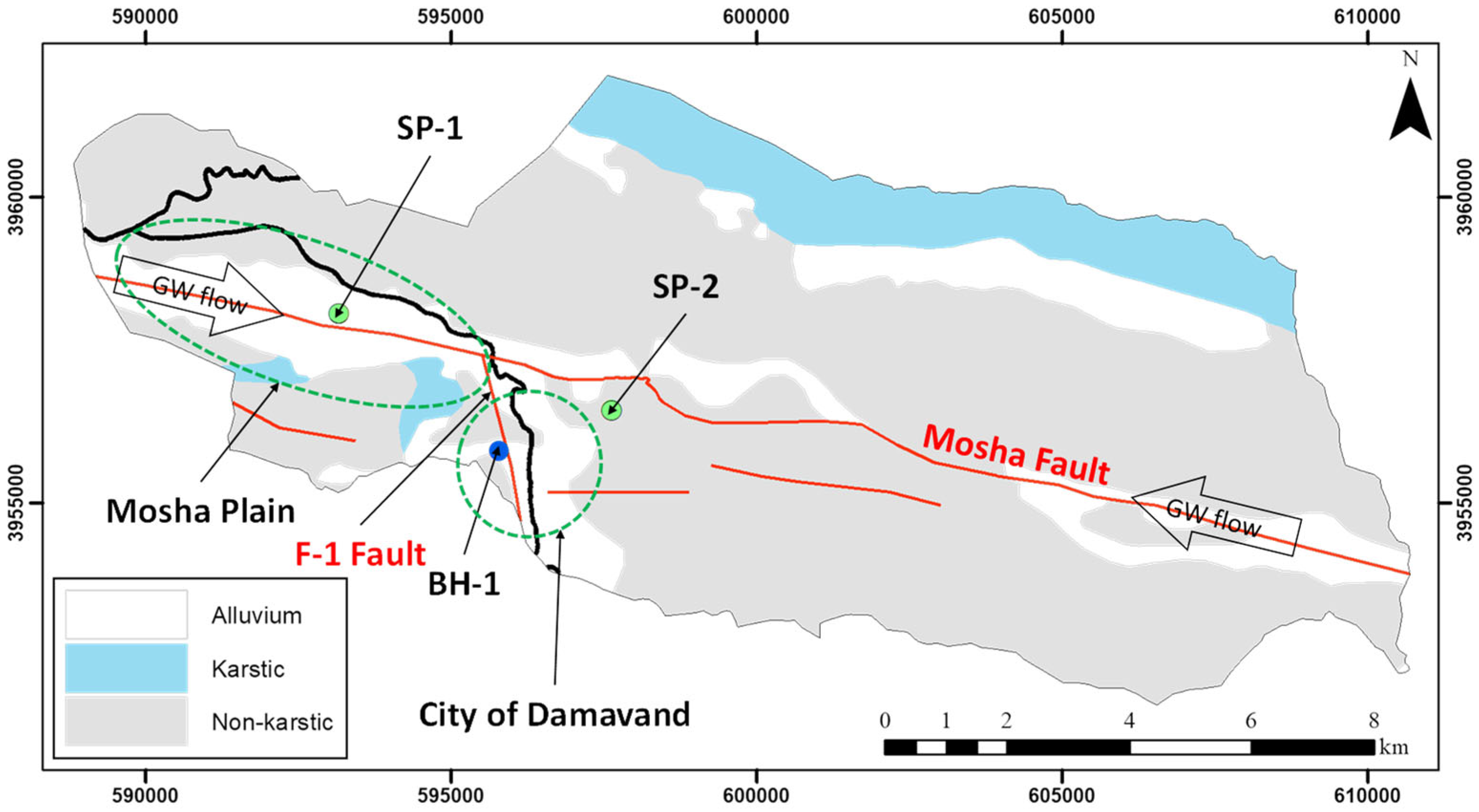
The Mosha aquifer, which is located in the Alborz zone in the north of Iran, consists of various geological formations with different karstification potentials, which have been affected by active faults, especially the Mosha Fault (Figure 1). The Mosha aquifer is a multi-layered setting in which non-developed karstic rocks, fractured sedimentary rocks, and alluvial sediments in the northern parts create the local groundwater recharge regions. However, probably the aquifer is being fed to a small extent from the southern part (Figure 2). The Mosha Fault, which is a basement-involved thrust (Figure 2), is the most prominent structure in the study area [46]. A significant number of springs and boreholes are located within the Mosha Fault zone as well. Therefore, this fault appears to play a crucial role in the emergence of springs. Consequently, the Mosha Fault zone is a major groundwater passage in the study area.
The Mosha Plain study area is located in a marginal climate zone, where the northern section of the river catchment is of the very wet climate type, but the southern section is of the wet climate type. Regarding the long-term meteorological data (2015–2019), the annual average air temperature and average annual precipitation are 13.35 °C and 394.3 mm, respectively [47]. The average depth of the groundwater level in alluvial and fractured rock aquifers is 12.4 and 19.8 m, respectively. Considering the water table in the wells and the surface topography, the general groundwater flow direction follows the Mosha Fault zone and the F-1 Fault zone southward (Figure 2).
Figure 2.
A map showing the karstic zones of the study area as well as the Mosha Fault and groundwater flow directions. Solid black lines represent major inter-city roads.
Figure 2.
A map showing the karstic zones of the study area as well as the Mosha Fault and groundwater flow directions. Solid black lines represent major inter-city roads.

The BH-1 borehole, which is located within the F-1 Fault zone, is the only well in the study area that is equipped with a data logger and records the groundwater temperature, water table fluctuations, and electrical conductivity on an hourly basis interval (Figure 2). The BH-1 borehole is about 80 m deep and withdraws the groundwater from the fractured rock aquifer. The BH-1 borehole data logger shows a significant increase in groundwater electrical conductivity (EC) after road-deicing campaigns (Figure 3). This results in unpredictable groundwater quality changes that increase water treatment costs.
3. Materials and Methods
Iran Water Resources Management Co. (IWRM) conducted a nationwide census of all groundwater resources during the period of 2010–2012. Regarding the census data, the information on 50 permanent springs (EC, pH, and temperature) and 303 wells is valid and reliable for the Mosha Plain study area. The following data were observed for each well: (1) well depth and depth to the water table, (2) total annual discharge, (3) groundwater electrical conductivity (EC) and temperature (T), and (4) groundwater acidity (pH). There are 236 wells located in the alluvial areas and 67 wells in the fractured rock aquifers.
The climatological data were downloaded from the Iran Meteorological Organization database [47], including the (1) daily precipitation height, (2) air daily average temperature, and (3) snowfall events (Figure 3).
Further, two additional sources were selected (SP-1 and SP-2, Table 1) and after a snowfall event in 2019, five samples were taken from each and analyzed for Na+, and Cl− concentrations as well as the electrical conductivity (EC) (Table 1). Flame photometry and titration methods were used to measure Na+, and Cl− concentrations, respectively.
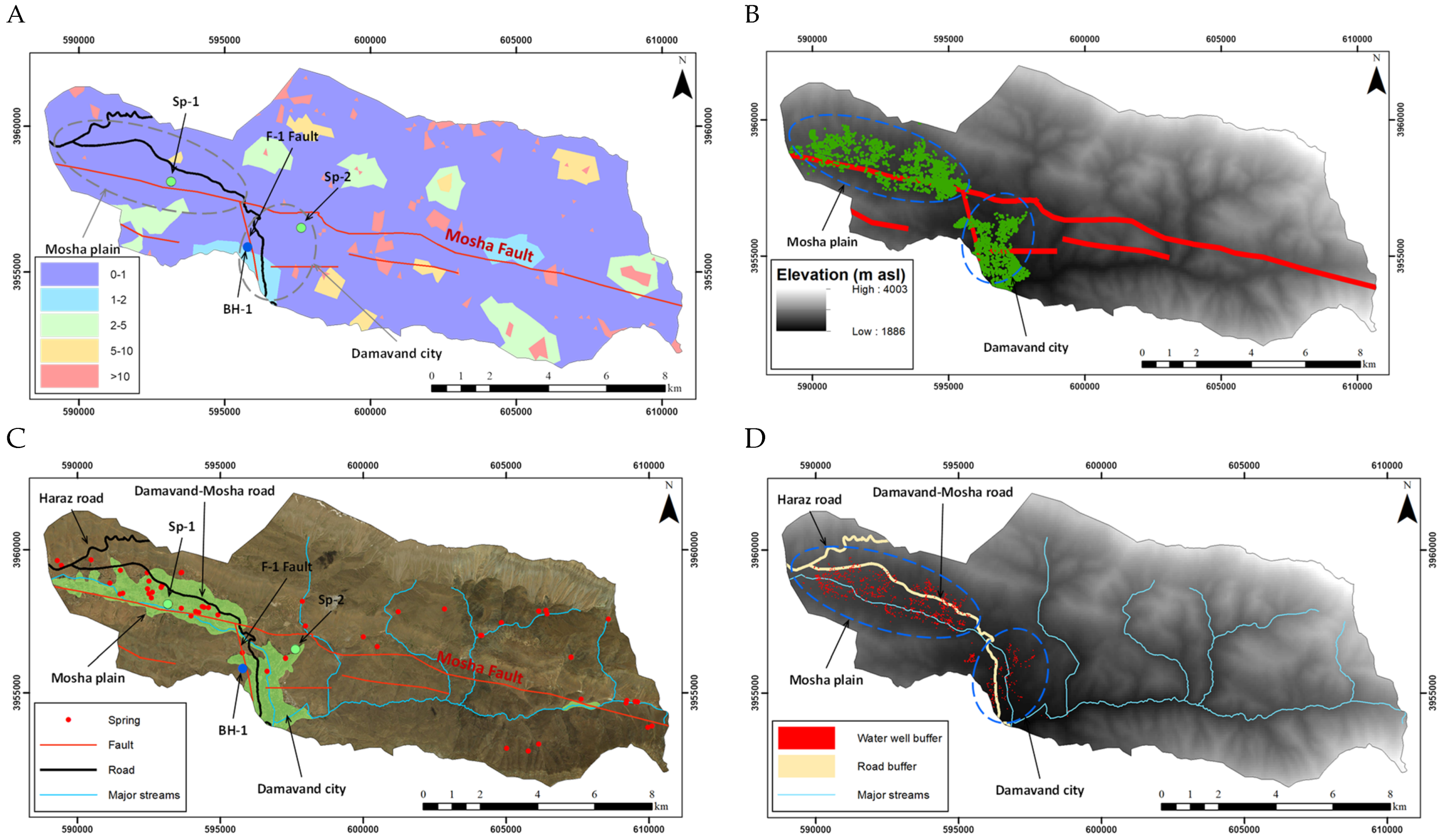
Mapping linear structures using remote sensing techniques is a principal approach in groundwater studies, especially in fractured rocky aquifers. In this study, the sign of fracture on the land surface is meant to be lineament. Initially, the lineament map was manually prepared using Landsat 8 satellite images in Envi 5.1 software. Then, using Landsat satellite images (Panchromatic bands), in the PCI Geomatica software environment, the lineaments were automatically extracted. Geomatica is a useful software program that uses an algorithm to analyze satellite images for features and fractures based on borders with different brightness and makes it possible to obtain the orientation and distribution of linear elements. However, the PCI Geomatica algorithm may mistakenly show roads, water channels, farms border, and crests as lineaments (pseudo-lineaments). Thus, the pseudo-lineaments were deleted from the map. Finally, using the Density function of the Spatial Analyst Tools in the ArcMap software, the maps for lineaments’ intensity were obtained (Figure 4A).
Unfortunately, there is no centralized municipal sewage collection system in the study area, and domestic wastewater gathers in private pit latrines and eventually leaks into the geological medium. In other words, each residential unit or residential complex has at least one pit latrine to collect municipal sewage. Municipal wastewater can be the source of a variety of pollutants such as nitrate, phosphate, salt, artificial sweeteners, fatty acids, hormones, etc. Therefore, it is necessary to study the effect of sewage absorption wells. For this, we produced the pit latrines using the Bing satellite image search engine (Figure 4B).

Table 1.
Results from chemical analysis of the samples taken after a snowfall event and following a road-deicing campaign in 2019.
Table 1.
Results from chemical analysis of the samples taken after a snowfall event and following a road-deicing campaign in 2019.
| Name | Date | EC (µS/cm) | Cl− (mg/L) | Na+ (mg/L) |
|---|---|---|---|---|
| BH-1 | 5 January 2019 | 670 | 86 | 23 |
| 6 January 2019 | 717 | 100 | 24 | |
| 7 January 2019 | 742 | 110 | 25.7 | |
| 9 January 2019 | 742 | 114 | 25.7 | |
| 16 January 2019 | 741 | 100 | 26.6 | |
| SP-1 | 5 January 2019 | 1452 | 300 | 123 |
| 6 January 2019 | 1116 | 160 | 46.2 | |
| 7 January 2019 | 1100 | 180 | 49.6 | |
| 9 January 2019 | 1119 | 186 | 48.4 | |
| 16 January 2019 | 1846 | 450 | 195 | |
| SP-2 | 5 January 2019 | 495 | 18 | 17.8 |
| 6 January 2019 | 288 | 10 | 15 | |
| 7 January 2019 | 521 | 20 | 11.2 | |
| 9 January 2019 | 500 | 20 | 10.6 | |
| 16 January 2019 | 495 | 20 | 10 |
Figure 4.
The maps indicate the groundwater vulnerability and hazard zones in the study area. Solid black lines represent major inter-city roads: (A) a map showing the fracture density in the study area (values are in fractures per m2); (B) the municipal pit latrines with a 50 m buffer zone; (C) a map showing the land use in the study area. The green patches show the municipal areas; (D) the groundwater abstraction wells with a 20 m buffer zone.

4. Results and Discussion
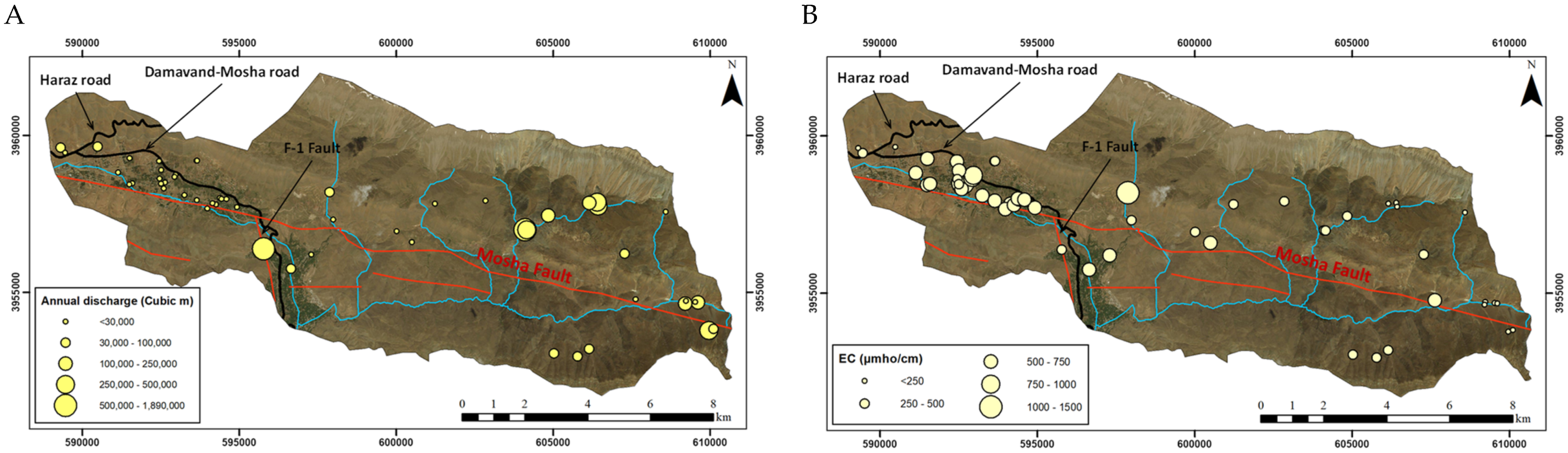
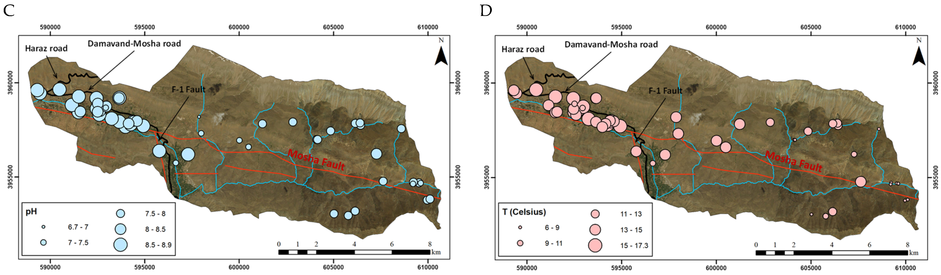
The distribution of the springs follows along the major geological structures (i.e., Mosha Fault) in the study area (Figure 4C). Therefore, the Mosha Fault appears to play a decisive role in the emergence of springs. The springs’ minimum and maximum annual discharges were 1339.2 and 1,892,160 m3, respectively. The minimum and maximum values for springs’ water electrical conductivity (EC) were 177 and 1450 µS/cm, respectively (Figure 5A,B). In addition, the lowest and highest levels of acidity (pH) were 6.7 and 8.9, respectively (Figure 5C). The annual average groundwater temperature was between 6 and 17.3 °C (Figure 5D). The springs’ water EC and temperature values were higher in the Mosha Plain, which may be an indication of the impact of rapid urbanization and urban wastewater leakage on the aquifer.
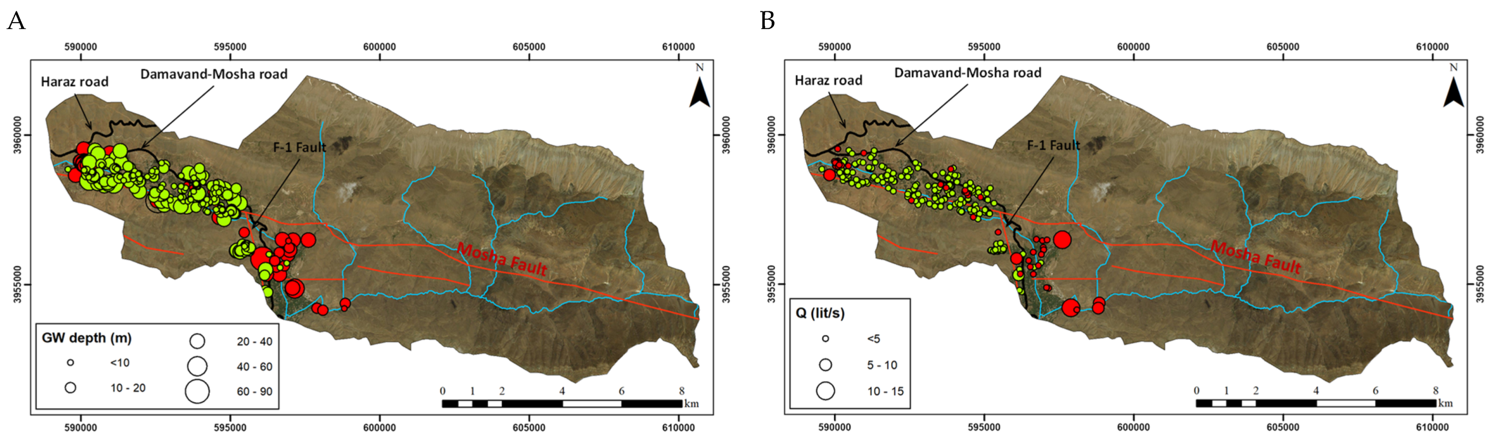
The average depth of the wells drilled in alluvium was about 19 m, and in the fractured rock, it was about 30 m. The average depths of the groundwater level in the alluvial and fractured rock aquifers were 12.4 and 19.8 m, respectively (Figure 6A). Additionally, the average annual groundwater discharge rates from the alluvial and fractured rock aquifers were approximately 556 and 19,128 m3, respectively (Figure 6B). The average electrical conductivity (EC) and acidity (pH) of the groundwater in the alluvial aquifer were about 588 µS/cm, and 7.6, respectively (Figure 6C,D). Further, the average EC and pH of the groundwater in the fractured rock aquifer were very close to those of the alluvial aquifer (EC ≈ 501 µS/cm, and pH ≈ 7.6). Most of the wells (both alluvial aquifer wells and the wells penetrated in the fractured rock aquifer) are within the Mosha Fault zone. Regarding the depth of the wells, it seems that the groundwater level in the northern parts of the Mosha Fault zone is shallower than in the southern parts (Figure 6).
The annual groundwater discharge rates by wells in the fractured rock and alluvial aquifers were about 1.28 and 0.13 MCM (million cubic meters), respectively. Generally, boreholes with high annual discharge volumes are located within the Mosha Fault zone (Figure 6).
Figure 6.
Quantitative and qualitative characteristics of the groundwater abstraction wells in the study area (green and red circles show the wells in the alluvial and fractured rock aquifers, respectively). Solid black lines represent major inter-city roads: (A) the groundwater depth in the wells; (B) the wells’ yield; (C) the groundwater electrical conductivity in the wells; (D) the groundwater acidity in the wells.


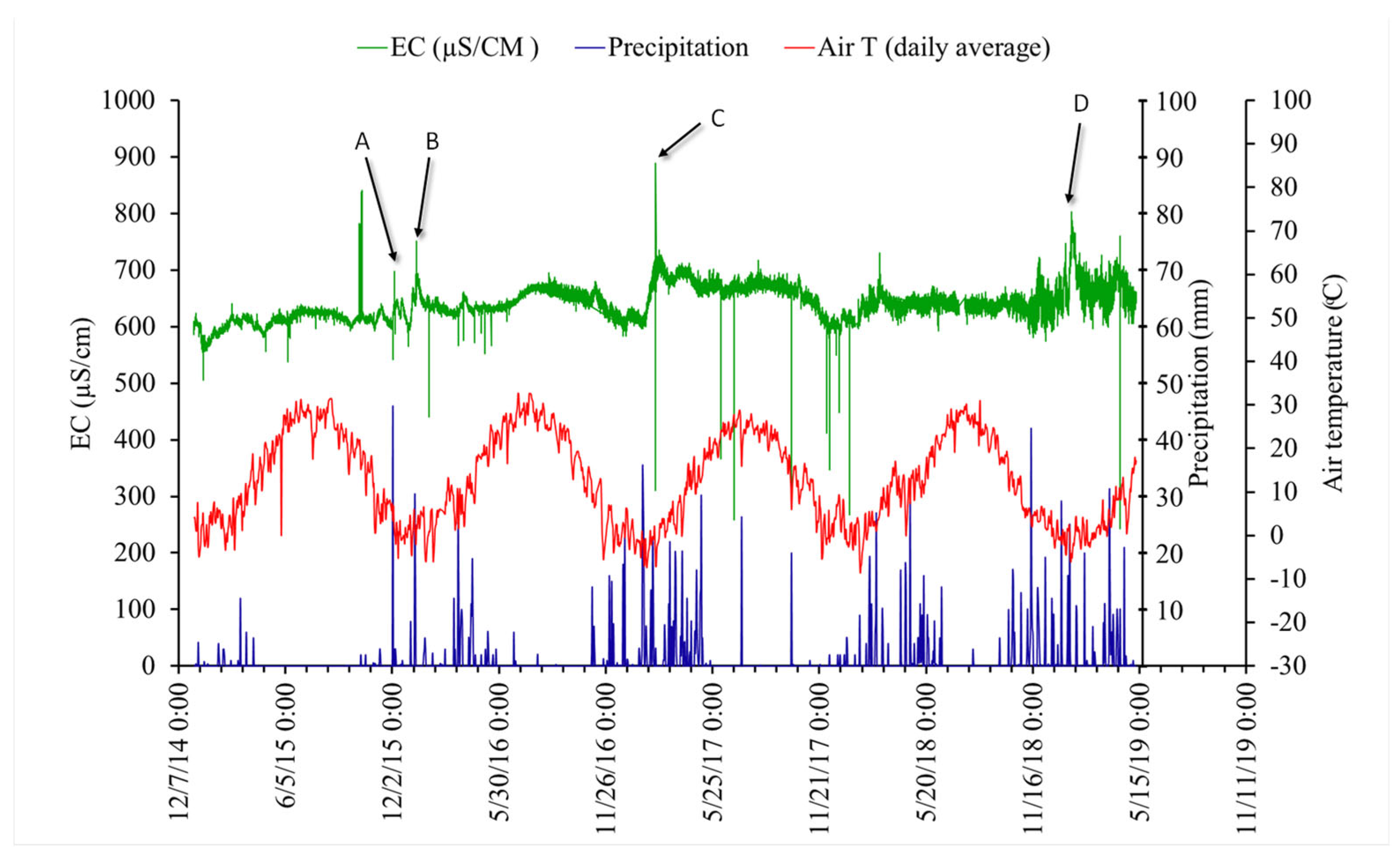
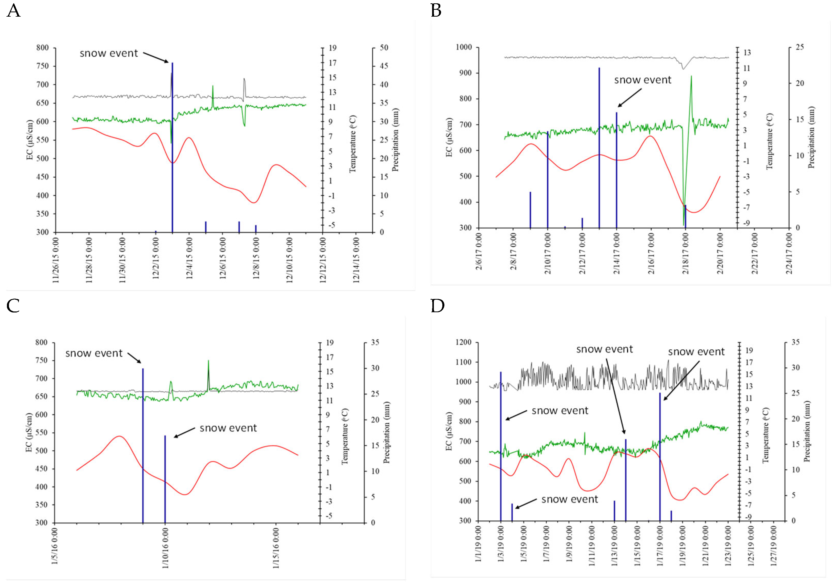
The groundwater electrical conductivity values in the BH-1 borehole historical data had several significant peaks during the winter time (Figure 3). Considering the freezing air temperature and the reported snow events as well as road-deicing campaigns, the periods during which the groundwater was potentially affected by salts were extracted (points A to D in Figure 3). Then, they were re-plotted in separate diagrams for further detailed studies (Figure 7). The study results show that the groundwater EC in the BH-1 increased after 1–4 days from a significant snow event and the subsequent road-deicing campaigns (Figure 7A,B). Additionally, there was a decrease in the groundwater EC about 4–7 days after a significant snowfall, which might be due to non-defrosted snowmelt infiltration (Figure 7A). Further, there were several high EC peaks after successive significant storm events (Figure 7C,D). Additionally, the groundwater EC gradually increased, which might be a result of the delayed approach of further molten snow from the road-defrosting operations (Figure 7C,D). Although there are no data about the aquifers’ hydraulic conductivity, regarding the BH-1 location, which is located within the F-1 Fault zone, it is anticipated that the hydraulic conductivity would be high along the fault-damaged zone (in the range of gravel and/or coarse sand). Therefore, given the lag time between snow events (and subsequent road-defrosting operations) and increased groundwater electrical conductivity in the BH-1, the source of groundwater contaminants is probably within 1–4 km of the well.
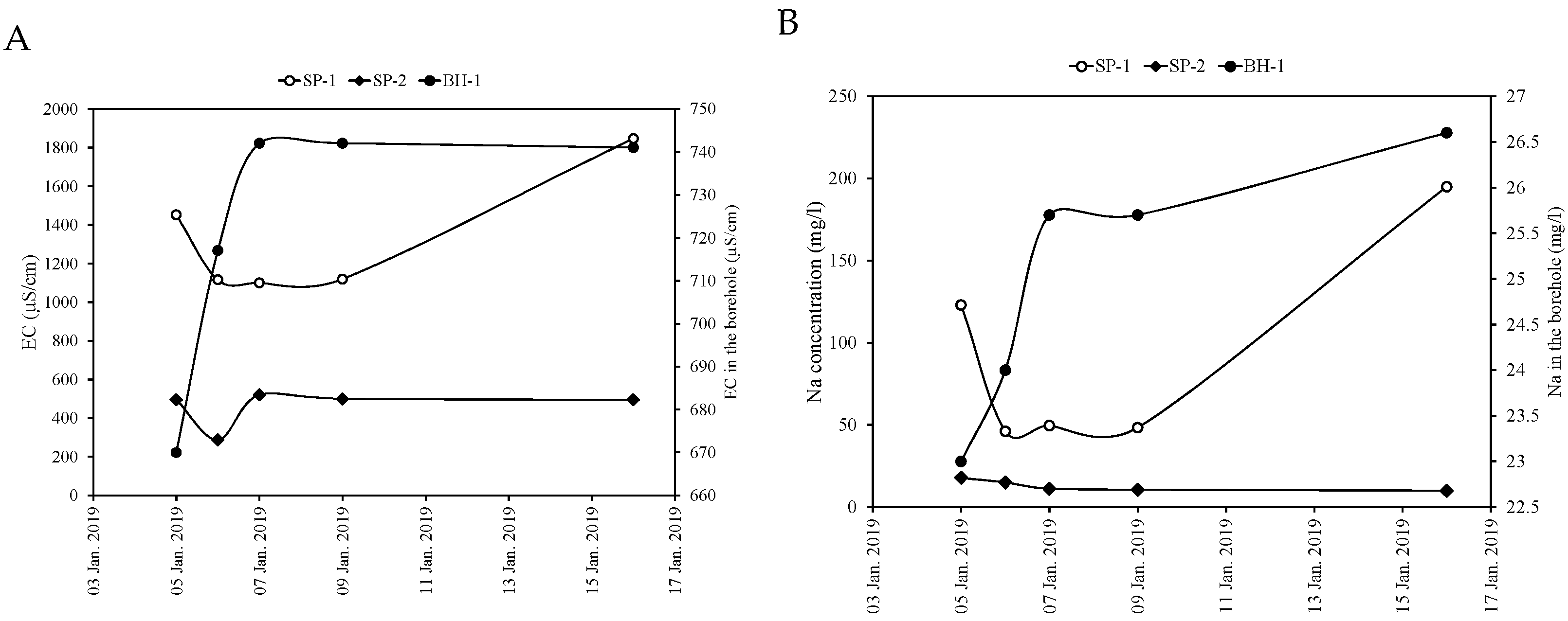
The results of the BH-1 and spring chemical analysis (Table 1) showed that the groundwater EC, and Na+ and Cl- concentrations increased in the BH-1 earlier than in the springs (Figure 8). Therefore, the BH-1 responded to the road-defrosting campaigns earlier than the sampled springs. The electrical conductivity and the concentration of Cl- and Na+ in the SP-1 spring increased with a delay compared with the BH-1, but the SP-2 spring did not respond to the road-deicing campaigns, as there was no obvious change in the chemical characteristics of the SP-2. Therefore, it seems that the source of groundwater contaminants is probably within 1–5 km of the SP-1 spring. Regarding the groundwater flow directions (Figure 2) and the response order of the BH-1 and springs, the following observations were clearly made:
- Initially, the groundwater contaminant reached the BH-1 from an area located between the BH-1 and SP-1;
- Then, some amount of salt approached the SP-1 from the west of the spring;
- Finally, the contaminants were diluted when the groundwater flowed from the SP-1 area toward the BH-1. This means that some amount of salt reached the BH-1 from the most western areas of the SP-1 with some delay.
Figure 7.
The impact of road-deicing campaigns on groundwater in the BH-1 (blue bars represent the precipitation events; red, green, and black lines are daily average air temperature, groundwater EC, and groundwater temperature, respectively): (A) single snow event in the year 2015; (B) single snow event in the year 2017; (C) multiple snow events in the year 2016; (D) multiple snow events in the year 2019.

In the hydrogeologic system of the Mosha Plain study area, vulnerability means a medium that may be susceptible to infiltration to link surface water to groundwater, and thus transfer poor-quality surface water into the groundwater system. Therefore, considering the available data in the Mosha Plain, the vulnerability factors are (1) the lithology of the study area; (2) the major structural geology features (e.g., faults, etc.) in the study area; and (3) the minor structural geology characteristics of the catchment, including the lineaments’ density.
Each vulnerable factor may consist of several segments that have distinct impacts on the hydrogeologic system susceptibility. A coefficient (C) is assigned to each segment, which is proportional to the amount of impact that segment has on the vulnerability of that factor. For example, in the lithology map, the formations are separated by type (alluvial, karstic, and non-karstic), and each is given a coefficient that is proportional to the type of effect the formation has on the aquifer vulnerability (Table 2). The closer it is to number 1, the greater the degree of its importance.
Figure 8.
Results of the groundwater samples taken from the BH-1 borehole, SP-1, and SP-2 springs during winter 2019. Snow events were on 3 and 4 January 2019 (see Figure 7D): (A) the groundwater samples’ EC changes; (B) the groundwater samples’ Na+ changes; (C) the groundwater samples’ Cl− changes.


Within the study area, the most potentially karstified formations are located along the northern border of the basin, which is potentially the aquifer’s recharge zone (Figure 2). Therefore, the leakage of the contaminant into the ground/surface within the recharge zone can quickly reach the aquifer and contaminate groundwater. This is basically because of the rapid infiltration of the recharging water (as well as the contaminants) into the aquifer. However, the groundwater flow direction may assist the pollutants to reach the saturated zone, especially in the southern parts of the basin, where the carbonate rocks are very close to the Mosha Fault zone. Therefore, the highest coefficient was given to the potentially karstified areas (Ck = 1). Most of the alluvial layers are located within the valleys and fault zones. In addition, the groundwater level in the alluvial aquifer (Masha Plain) appears to be shallow, which increases the vulnerability of the alluvial aquifer. Therefore, the alluvial layers coefficient was determined as 0.7 (Call = 0.7). The non-karstic formations in the study area not only have low permeability but also have no groundwater-quality degrading layers. Therefore, the lowest coefficient was given to the non-karstic layers (Cnon-k = 0.5).
The main fault in the study area is the Mosha Fault, which has an east–west trend (Figure 2). This fault and its branched faults are the main channels of groundwater. Furthermore, these fault-damaged zones are passages through which the groundwater may leak from the alluvial aquifer into the fractured rock aquifer or vice versa. In addition, the Mosha Fault has a wide fault zone. Therefore, for these faults, a buffer of 100 m was considered (Table 2 and Figure 4B). This buffer zone indicates a vulnerable area that is greatly susceptible to the contaminants that may penetrate into the groundwater.
Table 2.
The inventory of layers and their assigned weight for the risk maps.
| Layer Name | Type | Weight | Buffer (m) | |
|---|---|---|---|---|
| Dry Season | Wet Season | |||
| Lithology | Vulnerability | 2 | 2 | - |
| Major structural features | 7 | 7 | 100 | |
| Minor structural features | 2 | 2 | - | |
| Sewage absorption wells | Hazard | 9 | 5 | 50 |
| Roads | 1 | 4 | 50 | |
| Groundwater abstraction boreholes | 1 | 1 | 20 | |
| Landuse | 2 | 5 | - | |
In fractured rock aquifers, fractures play an important role in groundwater transport. Accordingly, the greater the number of fractures in an area, the greater the vulnerability to leakage of surface contaminants. The extracted lineaments are macro-fractures that are visible in the applied Landsat images. This means that these fractures are deep enough to transmit meteoric water and the accompanying contaminants into the aquifer. A lineament density map shows the number of fractures per unit area. Here, the lineament density map is reproduced using the lineament map that shows the number of fractures per square kilometer (Figure 4A). However, in order to use this map to calculate the vulnerability map, the numbers must be proportional to 1. In other words, the density of the lineaments should be between 0 and 1. For this reason, the largest lineament density was considered to be 1, and the rest of the density values were calculated accordingly. As a result, the closer the numbers are to one, the greater the line density, and the aquifer in those parts becomes more vulnerable.
In the Mosha Plain study area, there are several hazard agents: (1) pit latrines; (2) roads; (3) groundwater abstraction boreholes; and (4) land use. Unfortunately, there is no centralized municipal sewage collection system in the study area, and domestic wastewater gathers in private pit latrines and eventually leaks into the geological medium. In other words, each residential unit or residential complex has at least one pit latrine to collect municipal sewage. Additionally, the Mosha Plain is mostly of a recreational nature, and its population increases during summer periods. Therefore, the contamination from pit latrines greatly increases in summer. A pit latrine map was prepared using the Bing satellite image search engine. For this purpose, a pit latrine was assumed for each residential unit. Since most of the pit latrines were drilled in alluvium, the wells were then subjected to a 50 m buffer, indicating the radius of the impact of each well (Table 2 and Figure 4B).
In the study area, land use includes the following two types (Figure 4C): (1) agriculture, which is more of a gardening type, including villas where most buildings occupy a small portion of the entire land area, and most of the land is devoted to the garden. In this type of land use, different types of fertilizers and pesticides are used and may contaminate the aquifer. It should be noted that the effect of the residential units and buildings was considered in the sewage well section; and (2) pasture with very poor vegetation, which has no role in groundwater pollution.
The main roads are mostly located in the western section of the study area. Roads may be subject to defrosting campaigns during winter. The drainage systems for collecting saline snow melt are not properly designed and can result in the infiltration of saline water and other pollutants into the aquifer. Therefore, given the fact that these roads are highways, and the volume of traffic is considerable, their potential for contamination is very high. For this purpose, a 50 m buffer range was set for the roads (Figure 4D). In fact, this buffer range reflects the impact radius of the roads and the extent to which various pollutants may penetrate the aquifer.
Groundwater wells, because they directly infiltrate into the aquifer, can quickly transport various pollutants into the aquifer. Contaminant transport through the well into the aquifer is intensified when the well (1) does not have a building, (2) uses fossil fuel, and (3) the design of the well is not correct. In the study area, almost all the wells are without buildings and are outdoors. In addition, the wells were built by non-professionals at a low cost. Therefore, they are not properly designed and can easily transport pollutants from the surface into the aquifer. Additionally, because most of them use electricity, they are less likely to leak fossil fuel pollutants into the aquifer. However, most are within the areas of villas and personal gardens and may leak fertilizers and pesticides into the aquifer. In wells, because the groundwater flows from the aquifer into the well, the spread of pollution is slow. For this reason, a 20 m buffer was used to evaluate and apply the impact of the wells on groundwater quality (Figure 4D). Thus, up to a radius of 20 m for each well was considered as the impact radius of the same well.
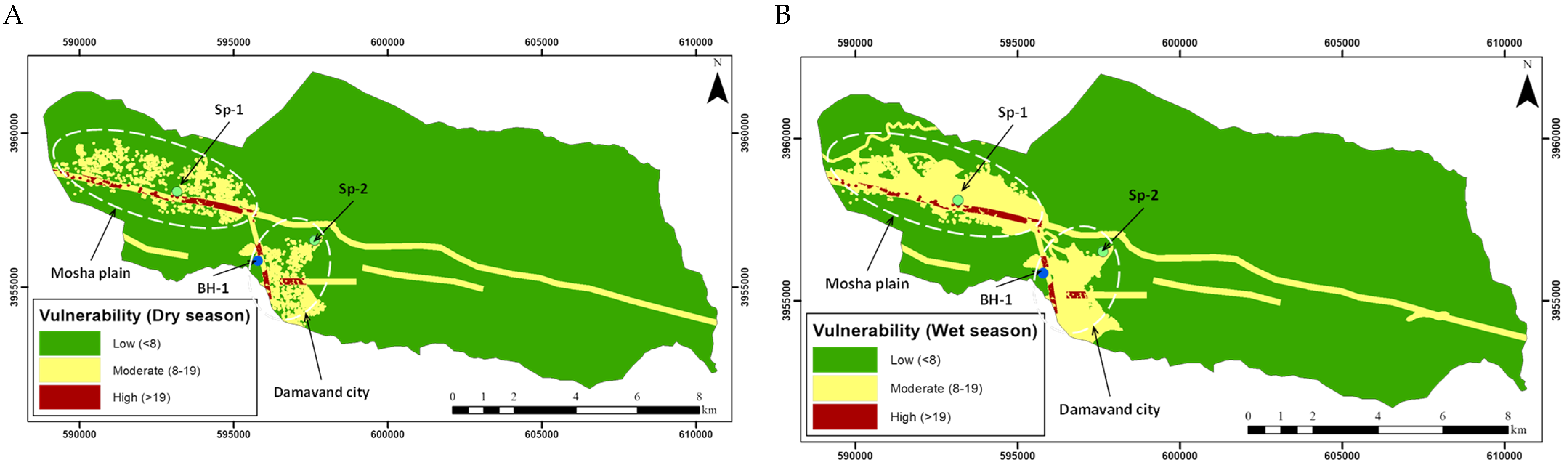
Due to the large number of summer cottages in this recreational area, its population is smaller in the fall and winter seasons (wet season). Therefore, the detrimental effect of sewage wells on groundwater quality is higher in the wet season (Table 2). Additionally, as road defrosting is carried out in winter, the weight of the road layer is higher for the wet season than in the dry season (Table 2). In gardens, most fertilization is usually carried out in the wet season. Subsequently, the fertilizers may be washed out of the root zone during the wet season and contaminate the groundwater. Therefore, the weight of the land use is higher in risk maps for the wet season than for the dry season (Table 2). The weight of the other vulnerability and hazard maps did not change for the wet or dry seasons (Table 2). Accordingly, the groundwater risk maps were prepared separately for the wet and dry seasons in the study area (Figure 9).
5. Conclusions
Our results show that the BH-1 borehole is very responsive to surficial contaminants. Moreover, the impact of the road-defrosting campaigns on the groundwater is significant in the study area, and the local anthropogenic contaminants that percolate the aquifer within the determined zone of contribution may reach the borehole within a few days. However, the penetrated saline snowmelt becomes diluted very quickly, and the groundwater EC reaches its base level soon after the elevated peaks. Further, most of the contaminant leakage occurs in the area of Mosha Plain and Damavand City as well as in the western part of the fault. In addition, although the distribution of risky points and areas may slightly change from wet to dry seasons, the general shape of the high-risk patches is almost the same (with the exception of the effect of roads in the northwestern part of the Mosha Plain). It seems that roads and sewage absorption wells have the biggest role in groundwater contamination in the study area.
Author Contributions
Conceptualization, Y.N. and V.N.; methodology, Y.N.; software, V.N.; validation, V.N., R.D. and A.R.; formal analysis, V.N.; investigation, Y.N.; resources, V.N. and R.D.; data curation, V.N.; writing—original draft preparation, Y.N. and V.N.; writing—review and editing, R.D. and A.R.; visualization, V.N.; supervision, Y.N.; project administration, Y.N.; funding acquisition, R.D. All authors have read and agreed to the published version of the manuscript.
Funding
This research received no external funding.
Data Availability Statement
Not applicable.
Conflicts of Interest
The authors declare no conflict of interest.
References
- Mohammadi, K.; Niknam, R.; Majd, V.J. Aquifer vulnerability assessment using GIS and fuzzy system: A case study in Tehran–Karaj aquifer, Iran. Environ. Geol. 2009, 58, 437–446. [Google Scholar] [CrossRef]
- Shirazi, S.M.; Akib, S.; Salman, F.A.; Alengaram, U.J.; Jameel, M. Agro-ecological aspects of groundwater utilization a case study. Sci. Res. Essays 2010, 5, 2786–2795. [Google Scholar] [CrossRef]
- Dimitriou, E.; Moussoulis, E. Land use change scenarios and associated groundwater impacts in a protected peri-urban area. Environ. Earth Sci. 2010, 64, 471–482. [Google Scholar] [CrossRef]
- Khan, H.H.; Khan, A.; Ahmed, S.; Perrin, J. GIS-based impact assessment of land-use changes on groundwater quality: Study from a rapidly urbanizing region of South India. Environ. Earth Sci. 2011, 63, 1289–1302. [Google Scholar] [CrossRef]
- Razandi, Y.; Pourghasemi, H.R.; Neisani, N.S.; Rahmati, O. Application of analytical hierarchy process, frequency ratio, and certainty factor models for groundwater potential mapping using GIS. Earth Sci. Inform. 2015, 8, 867–883. [Google Scholar] [CrossRef]
- Kumar, A.; Pandey, A.C. Geoinformatics based groundwater potential assessment in hard rock terrain of Ranchi urban environment, Jharkhand state (India) using MCDM–AHP techniques. Groundw. Sustain. Dev. 2016, 2–3, 27–41. [Google Scholar] [CrossRef]
- Zektser, I.; Karimova, O.; Bujuoli, J.; Bucci, M. Regional estimation of fresh groundwater vulnerability: Methodological aspects and practical applications. Water Resour. 2004, 31, 595–600. [Google Scholar] [CrossRef]
- Causapé, J.; Quílez, D.; Aragüés, R. Groundwater quality in CR-V irrigation district (Bardenas I, Spain): Alternative scenarios to reduce off-site salt and nitrate contamination. Agric. Water Manag. 2006, 84, 281–289. [Google Scholar] [CrossRef]
- Chenini, I.; Zghibi, A.; Kouzana, L. Hydrogeological investigations and groundwater vulnerability assessment and mapping for groundwater resource protection and management: State of the art and a case study. J. Afr. Earth Sci. 2015, 109, 11–26. [Google Scholar] [CrossRef]
- Fobe, B.; Goossens, M. The groundwater vulnerability map for the Flemish region: Its principles and uses. Eng. Geol. 1990, 29, 355–363. [Google Scholar] [CrossRef]
- Worrall, F.; Besien, T. The vulnerability of groundwater to pesticide contamination estimated directly from observations of presence or absence in wells. J. Hydrol. 2005, 303, 92–107. [Google Scholar] [CrossRef]
- Gogu, R.C.; Dassargues, A. Current trends and future challenges in groundwater vulnerability assessment using overlay and index methods. Environ. Geol. 2000, 39, 549–559. [Google Scholar] [CrossRef]
- Frind, E.O.; Molson, J.W.; Rudolph, D.L. Well vulnerability: A quantitative approach for source water protection. Groundwater 2006, 44, 732–742. [Google Scholar] [CrossRef]
- Zghibi, A.; Merzougui, A.; Chenini, I.; Ergaieg, K.; Zouhri, L.; Tarhouni, J. Groundwater vulnerability analysis of Tunisian coastal aquifer: An application of DRASTIC index method in GIS environment. Groundw. Sustain. Dev. 2016, 2–3, 169–181. [Google Scholar] [CrossRef]
- Javadi, S.; Kavehkar, N.; Mohammadi, K.; Khodadadi, A.; Kahawita, R. Calibrating DRASTIC using field measurements, sensitivity analysis and statistical methods to assess groundwater vulnerability. Water Int. 2011, 36, 719–732. [Google Scholar] [CrossRef]
- Nobre, R.C.; Rotunno Filho, O.C.; Mansur, W.J.; Nobre, M.M.; Cosenza, C.A. Groundwater vulnerability and risk mapping using GIS, modeling and a fuzzy logic tool. J. Contam. Hydrol. 2007, 94, 277–292. [Google Scholar] [CrossRef]
- Liggett, J.E.; Talwar, S. Groundwater vulnerability assessments and integrated water resource management. Streamline Watershed Manag. Bull. 2009, 13, 18–29. [Google Scholar]
- McLay, C.D.A.; Dragten, R.; Sparling, G.; Selvarajah, N. Predicting groundwater nitrate concentrations in a region of mixed agricultural land use: A comparison of three approaches. Environ. Pollut. 2001, 115, 191–204. [Google Scholar] [CrossRef]
- Iqbal, J.; Gorai, A.; Tirkey, P.; Pathak, G. Approaches to groundwater vulnerability to pollution: A literature review. Asian J. Water Environ. Pollut. 2012, 9, 105–115. [Google Scholar]
- Almasri, M.N. Assessment of intrinsic vulnerability to contamination for Gaza coastal aquifer, Palestine. J. Environ. Manag. 2008, 88, 577–593. [Google Scholar] [CrossRef]
- Aller, L.; Bennet, T.; Lehr, J. A Standardized System for Evaluating Ground Water Pollution Potential Using Hydrogeological Settings; US Environmental Protection Agency: Ada, OK, USA, 1987. [Google Scholar]
- Foster, S. Fundamental concepts in aquifer vulnerability, pollution risk and protection strategy. In Proceedings of the Vulnerability of Soil and Groundwater to Polluants, International Conference, Noordwijk, The Netherlands, 30 March 1987. [Google Scholar]
- Civita, D.M. Le Carte Della Vulnerabilità Degli Acquiferi All’inquinamento: Teoria e Pratica; Pitagora: Bolonga, Italy, 1994. [Google Scholar]
- Doerfliger, N.; Zwahlen, F. EPIK: A new method for outlining of protection areas in karstic environment. In Proceedings of the International Symposium and Field Seminar on “Karst Waters and Environmental Impacts”, Antalya, Turkey, 10–20 September 1995; Günay, G., Jonshon, A.I., Eds.; Balkema: Rotterdam, The Netherlands, 1995; pp. 117–123. [Google Scholar]
- Navulur, K.; Engel, B. Groundwater vulnerability assessment to non-point source nitrate pollution on a regional scale using GIS. Trans. ASAE 1998, 41, 1671–1678. [Google Scholar] [CrossRef]
- Fernández, D.S.; Lutz, M.A. Urban flood hazard zoning in Tucumán Province, Argentina, using GIS and multicriteria decision analysis. Eng. Geol. 2010, 111, 90–98. [Google Scholar] [CrossRef]
- Rebolledo, B.; Gil, A.; Flotats, X.; Sanchez, J.A. Assessment of groundwater vulnerability to nitrates from agricultural sources using a GIS-compatible logic multicriteria model. J. Environ. Manag. 2016, 171, 70–80. [Google Scholar] [CrossRef] [Green Version]
- Seekao, C.; Pharino, C. Assessment of the flood vulnerability of shrimp farms using a multicriteria evaluation and GIS: A case study in the Bangpakong Sub-Basin, Thailand. Environ. Earth Sci. 2016, 75, 308. [Google Scholar] [CrossRef]
- Pollock, S. Mitigating highway deicing salt contamination of private water supplies in Massachusetts. In Research and Materials Section; Massachusetts Department of Public Works: Wellesley, MA, USA, 1990. [Google Scholar]
- Thunqvist, E.L. Regional increase of mean chloride concentration in water due to the application of deicing salt. Sci. Total Environ. 2004, 325, 29–37. [Google Scholar] [CrossRef]
- Kaushal, S.S.; Groffman, P.M.; Likens, G.E.; Belt, K.T.; Stack, W.P.; Kelly, V.R.; Band, L.E.; Fisher, G.T. Increased salinization of fresh water in the northeastern United States. Proc. Natl. Acad. Sci. USA 2005, 102, 13517–13520. [Google Scholar] [CrossRef] [Green Version]
- Chapra, S.C.; Dove, A.; Rockwell, D.C. Great Lakes chloride trends: Long-term mass balance and loading analysis. J. Great Lakes Res. 2009, 35, 272–284. [Google Scholar] [CrossRef]
- Mullaney, J.R.; Lorenz, D.L.; Arntson, A.D. Chloride in groundwater and surface water in areas underlain by the glacial aquifer system. North. U. S. Sci. Investig. Rep. 2009, 5086, 41. [Google Scholar]
- Likens, G.E.; Buso, D.C. Salinization of Mirror Lake by Road Salt. Water Air Soil Pollut. 2010, 205, 205–214. [Google Scholar] [CrossRef]
- Dailey, K.R.; Welch, K.A.; Lyons, W.B. Evaluating the influence of road salt on water quality of Ohio rivers over time. Appl. Geochem. 2014, 47, 25–35. [Google Scholar] [CrossRef]
- Rogora, M.; Mosello, R.; Kamburska, L.; Salmaso, N.; Cerasino, L.; Leoni, B.; Garibaldi, L.; Soler, V.; Lepori, F.; Colombo, L.; et al. Recent trends in chloride and sodium concentrations in the deep subalpine lakes (Northern Italy). Environ. Sci. Pollut. Res. Int. 2015, 22, 19013–19026. [Google Scholar] [CrossRef] [PubMed] [Green Version]
- Sibert, R.J.; Koretsky, C.M.; Wyman, D.A. Cultural meromixis: Effects of road salt on the chemical stratification of an urban kettle lake. Chem. Geol. 2015, 395, 126–137. [Google Scholar] [CrossRef]
- Wyman, D.A.; Koretsky, C.M. Effects of road salt deicers on an urban groundwater-fed kettle lake. Appl. Geochem. 2018, 89, 265–272. [Google Scholar] [CrossRef]
- Dennis, H.W. Salt Pollution of a Shallow Aquifer—Indianapolis, Indiana. Groundwater 1973, 11, 18–22. [Google Scholar] [CrossRef]
- Angel, D.R. Winter Deicing Effects on Groundwater Quality Beneath Permeable Asphalt. Master’s Thesis, University of Connecticut, Storrs, CT, USA, 2015. [Google Scholar]
- Rivett, M.O.; Cuthbert, M.O.; Gamble, R.; Connon, L.E.; Pearson, A.; Shepley, M.G.; Davis, J. Highway deicing salt dynamic runoff to surface water and subsequent infiltration to groundwater during severe UK winters. Sci. Total Environ. 2016, 565, 324–338. [Google Scholar] [CrossRef] [Green Version]
- Backstrom, M.; Karlsson, S.; Backman, L.; Folkeson, L.; Lind, B. Mobilisation of heavy metals by deicing salts in a roadside environment. Water Res. 2004, 38, 720–732. [Google Scholar] [CrossRef]
- McNaboe, L. Impacts of De-Icing Salt Contamination of Groundwater in a Shallow Urban Aquifer. Master’s Thesis, University of Connecticut Graduate School, Storrs, CT, USA, 2017. Available online: https://opencommons.uconn.edu/gs_theses/1138 (accessed on 1 July 2022).
- Dietz, M.E.; Angel, D.R.; Robbins, G.A.; McNaboe, L.A. Permeable Asphalt: A New Tool to Reduce Road Salt Contamination of Groundwater in Urban Areas. Groundwater 2017, 55, 237–243. [Google Scholar] [CrossRef] [PubMed]
- Reyahi Khoram, M.; Nafea, M.; Mahjub, H.; Hashemy, M.; Parchian, M. Effects of road deicing salt on the quality of ground water resources in Hamadan province, west of Iran. J. Res. Health Sci. 2011, 1, 39–44. [Google Scholar]
- Rashidi, A.; Derakhshani, R. Strain and Moment- Rates from GPS and Seismological Data in Northern Iran: Implications for an Evaluation of Stress Trajectories and Probabilistic Fault Rupture Hazard. Remote Sens. 2022, 14, 2219. [Google Scholar] [CrossRef]
- Iran Meteorological Organization Database. Available online: http://www.irimo.ir/index.php?newlang=eng (accessed on 18 May 2022).
Figure 1.
Geological map and cross-sections of the study area.

Figure 3.
The BH-1 groundwater EC historical data and climatological historical records in the nearest meteorological station (Iran Meteorological Organization database, 2019). Points A, B, C, and D represent the groundwater EC increase after road-deicing campaigns. Some very low points in EC are due to the removal of the probe from the well to perform well maintenance operations. In these cases, air fills the space between the electrodes of the electrical conductivity sensor, which is an electrical insulator. The rest of the cases are probably due to the operation of the pump in the well, which causes air bubbles in the water and causes errors in the measurement of EC.

Figure 5.
Quantitative and qualitative characteristics of springs in the study area. Solid black lines represent major inter-city roads: (A) the springs’ water annual discharge; (B) the springs’ water electrical conductivity; (C) the springs’ water acidity; (D) the springs’ water temperature.
Figure 5.
Quantitative and qualitative characteristics of springs in the study area. Solid black lines represent major inter-city roads: (A) the springs’ water annual discharge; (B) the springs’ water electrical conductivity; (C) the springs’ water acidity; (D) the springs’ water temperature.


Figure 9.
Risk maps of the Mosha Plain for the dry and wet seasons: (A) risk map of the dry season; (B) risk map of the wet season.
Figure 9.
Risk maps of the Mosha Plain for the dry and wet seasons: (A) risk map of the dry season; (B) risk map of the wet season.

Publisher’s Note: MDPI stays neutral with regard to jurisdictional claims in published maps and institutional affiliations. |
© 2022 by the authors. Licensee MDPI, Basel, Switzerland. This article is an open access article distributed under the terms and conditions of the Creative Commons Attribution (CC BY) license (https://creativecommons.org/licenses/by/4.0/).
Share and Cite
MDPI and ACS Style
Nikpeyman, Y.; Nikpeyman, V.; Derakhshani, R.; Raoof, A. Assessment of a Multi-Layer Aquifer Vulnerability Using a Multi-Parameter Decision-Making Method in Mosha Plain, Iran. Water 2022, 14, 3397. https://doi.org/10.3390/w14213397
AMA Style
Nikpeyman Y, Nikpeyman V, Derakhshani R, Raoof A. Assessment of a Multi-Layer Aquifer Vulnerability Using a Multi-Parameter Decision-Making Method in Mosha Plain, Iran. Water. 2022; 14(21):3397. https://doi.org/10.3390/w14213397
Chicago/Turabian StyleNikpeyman, Yaser, Vahid Nikpeyman, Reza Derakhshani, and Amir Raoof. 2022. "Assessment of a Multi-Layer Aquifer Vulnerability Using a Multi-Parameter Decision-Making Method in Mosha Plain, Iran" Water 14, no. 21: 3397. https://doi.org/10.3390/w14213397
Note that from the first issue of 2016, this journal uses article numbers instead of page numbers. See further details here.