An MLC and U-Net Integrated Method for Land Use/Land Cover Change Detection Based on Time Series NDVI-Composed Image from PlanetScope Satellite

Abstract

Land use/land cover change (LUCC) detection based on optical remote-sensing images is an important research direction in the field of remote sensing. The key to it is to select an appropriate data source and detection method. In recent years, the continuous expansion of construction land in urban areas has become the main reason for the increase in LUCC demand. However, due to the complexity and diversity of land-cover types, it is difficult to obtain high-precision classification results. In this article, a 12-month time series NDVI (Normalized Difference Vegetation Index) image of the study area was generated based on the high spatial and temporal resolution PlanetScope satellite images. According to the time series NDVI image, representative land-cover samples were selected, and the changed land samples were selected at the same time. This method could directly obtain the LUCC detection results of the study area through land-cover classification. First, Maximum Likelihood Classification (MLC), a classical machine-learning method, was used for supervised classification, and the samples needed for deep learning were selected according to the classification results. Then, the U-Net model, which can fully identify and explore the deep semantic information of the time series NDVI image, was used for land classification. Finally, this article made a comparative analysis of the two classification results. The results demonstrate that the overall classification accuracy based on time series NDVI is significantly higher than that of single-scene NDVI and mean NDVI. The LUCC detection method proposed in this article can effectively extract changed areas. The overall accuracy of the MLC and U-Net model is 79.38% and 85.26%, respectively. Therefore, the deep-learning method can effectively improve the accuracy of land-cover classification and change detection.

1. Introduction

Land use/land cover (LULC) information is essential for a region to carry out land-use planning, dynamic land monitoring, protection and management of cultivated land resources, etc. [1,2]. In order to improve the efficiency of land use and protect the ecological environment, it is necessary to master and update the existing land-cover information. The rapid development of remote-sensing technology and the progress of image-classification methods make large-area land cover information surveys possible. How to effectively apply massive remote-sensing information to obtain higher-precision land-cover classification has always been the direction of research efforts [3]. Land-classification research has been changing and updating with the development of data sources and extraction methods.

At present, there are many remote-sensing image datasets widely used in land-cover classification and change detection. Using the appropriate data source depends on the different research areas and classification purposes. MODIS, Landsat, Sentinel-2, and other medium-resolution remote-sensing images have the characteristics of wide coverage and high repeatability. These kinds of data are suitable for large-scale macro land-cover surveys and can be used to detect large areas of ground objects (e.g., forests, cultivated land, wetlands, and deserts) [4,5,6,7]. However, for some small spots that are easy to be missed, it is necessary to conduct additional surveys through field investigation. With the improvement in spatial resolution, the surface features presented by high-resolution remote-sensing images have become more detailed. The boundary of land spots can be defined more accurately. At present, the most commonly used high-resolution remote-sensing images for LULC classification include QuickBird, Worldview series, and GF series [8,9]. However, for the LULC survey, a higher resolution is not always better. Compared with low-resolution images, high-resolution images have a narrow coverage area, more noise, and a large number of phenomena of “different objects with the same spectral characteristics” [10], which increase the complexity of large-scale land classification. Therefore, high-resolution images are suitable for small-area research or monitoring small targets. For urban areas with complex and varied terrain types, automatically extracting the detailed LULC information from remote-sensing images is still very difficult. Medium-resolution images obviously cannot achieve the extraction of small image spots, and super-high-resolution images have high acquisition and computation costs. Therefore, this study adopts PlanetScope satellite images with medium-high resolution. The satellite revisits any part of the globe every day with a resolution of 3 m. It has the characteristics of wide coverage and fast update speed. Moreover, corrected orthophoto images can be obtained, which are suitable for LUCC monitoring [11,12,13,14].

NDVI is one of the most widely used Vegetation Indexes (VIs) at present. It can eliminate the influence of most instrument calibrations, the sun angle, terrain, cloud shadow, etc., and enhance the sensitivity to vegetation, which makes it an excellent indicator of vegetation growth states and vegetation coverage. In addition, vegetation cover is easily affected by seasonal changes and human activities. Therefore, using time series NDVI data can more accurately reflect the changing trend of vegetation cover in a period and effectively distinguish the spectral characteristics of different vegetation types [15,16]. Based on NDVI and the measured data of meteorological stations, it is a major direction of NDVI research to analyze the temporal changes of vegetation, climate, and human activities through correlation analysis, residual analysis, and other methods. For the further evaluation of the impact of climatic and anthropogenic factors on NDVI changes, the regional land-cover map is important auxiliary data [17,18,19]. In order to obtain an accurate LUCC map, a feasible way is to directly use time series NDVI for land-cover classification and then extract changed areas using a post-processing method. In addition, there are many studies devoted to fusing different satellite data. This method can fully integrate the advantages of spatial resolution and temporal resolution of different satellites so as to obtain a high-quality NDVI image after fusion [20]. Using fused time-series NDVI combined with original satellite images and phenological parameters extracted from NDVI can effectively improve the accuracy of land-cover classification. Nevertheless, it still sometimes fails to achieve good results due to the missing information of some months or regions and the deviation of model regression fitting [21,22] when compared with using other satellite data with a lower temporal resolution and adopting time-series fusion for time-series analysis. The time series NDVI derived from PlanetScope is realistic and avoids complex data processing, which can obtain a better result in a more efficient way.

Classical machine-learning classifiers mainly include MLC [23], Decision Tree [24], Random Forest [25], and Support Vector Machine [26]. These methods are based on the image texture, spectrum, and other information for classification. There are many studies comparing classical machine-learning approaches [27,28]. In the field of urban change detection, these machine-learning methods have been used by many scholars and have achieved relatively good results [29,30]. However, these shallow machine-learning methods cannot fully learn the deep semantic features of each land-cover type in remote-sensing images; it is often difficult to obtain good classification results for areas with complex land-cover information. In recent years, deep learning has made great progress. Compared with classical machine learning, deep learning has the advantages of being able to adaptively extract the most relevant features for classification tasks, fully excavate deeper feature information, and effectively obtain feature variables expressing land-cover information. Therefore, this technology has also been introduced into the field of LUCC surveys, which has become a popular research topic in the field of remote sensing [31,32]. At present, commonly used deep-learning models include convolutional neural networks (CNNs), recurrent neural networks (RNNs), and fully convolutional networks (FCN). Compared with CNN, FCNs solve the limitation of the fixed size of input and output images of CNN. In addition, it can reduce redundant calculations and improve the efficiency of large-scale LUCC mapping [33]. Classical FCN networks include U-Net, Deep-LAB, and PSP-Net, among which U-Net has a symmetric structure and only uses a small amount of training data to achieve relatively high accuracy. Therefore, U-Net is widely used in the field of remote-sensing image classification [34]. A large number of deep-learning samples need to be manually selected, which is very time- and energy-consuming. In order to reduce the workload, this article used the preliminary classification result obtained by MLC and the original satellite images to manually edit to obtain samples for deep learning.

In this article, a 12-month continuous time series NDVI image of the study area was acquired based on PlanetScope satellite products. The MLC and U-Net model were used for land-cover classification and change detection. Finally, the accuracy of the classification results was evaluated by satellite images and field survey data. The objectives of this study are: (1) to explore the effect of NDVI data from PlanetScope satellite products, which are rarely used at present in the application of real land-cover classification; (2) to analyze and compare the accuracy of MLC and U-Net models in LUCC detection using time series NDVI; (3) to propose a sample-selection method that selects samples according to MLC supervised classification results so as to improve the efficiency of deep-learning sample acquisition.

2. Materials and Methods

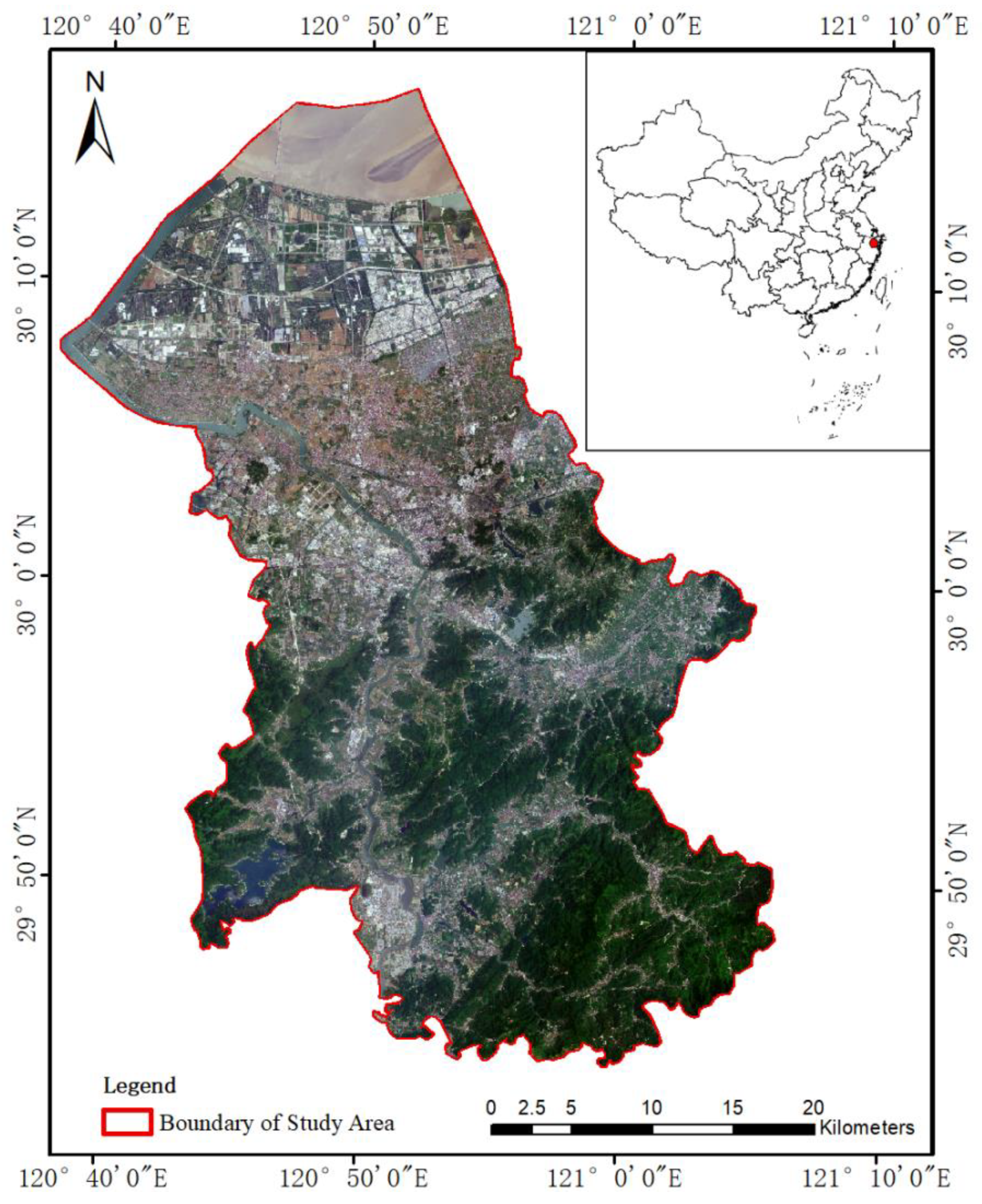
2.1. Study Area

The study area of this article is Shangyu district (29°43′38″−30°16′17″ N, 120°36′23″−121°06′09″ E), which is located in the northeast of Zhejiang Province, China (Figure 1). The basic outline of Shangyu is a north–south rectangle, covering a total area of about 1403 square kilometers, of which the Qiantang River estuary is 212.3 square kilometers. Shangyu’s terrain is high in the south and low in the north. The area of the southern low mountains and hills is basically the same as that of the northern water network and plain. The north, with an average altitude of about 5 m, has rich cultivated land resources and dense urban distribution, which is the key area for land classification. The southern region is rich in forest resources, with a small number of residential and agricultural lands staggered among them. Shangyu is a rapidly developing district in China’s coastal area, with large areas of reclamation land and a fast rate of LULC change. The demand for regional economic development led to the change of land, mainly from agricultural land and forest land to construction land. In general, the types of land cover in this area are complex and diverse, and the areas of various types are unbalanced. The traditional classification methods are not applicable in this area. Therefore, in order to effectively carry out land-use planning, it is necessary to select appropriate data sources and classification methods to obtain better land-cover classification and change-detection results.

2.2. Materials

The remote-sensing images used in this article are from PlanetScope satellites. PlanetScope small satellite constellation is the largest satellite constellation used for Earth observation in the world. The satellite consists of numerous Dove satellites equipped with remote-sensing observation equipment. The designed life expectancy of each satellite is about 3 years, which enables the satellite to be updated and replaced frequently. Currently, there are more than 170 satellites in orbit. Their products feature high temporal and spatial resolution and full coverage of the Earth. Specifically, the resolution of main image products acquired by the satellite sensor is about 3–4 m. The huge number of satellites and the extremely short revisit period enable it to cover any area of the world once a day [35,36]. Specific parameters are shown in

Table 1. PlanetScope satellite parameter information.

Parameter Name	Parameter Information
Image spectral range	Blue: 455~515 nm; Green: 500~590 nm; Red: 590~670 nm; NIR: 780~860 nm
Orbit name	International Space Station Orbit (ISS)	Solar Synchronous Orbit (SSO)
Orbit altitude	400 km	475 km
Orbit inclination	51.6°	−98°
Latitude coverage	±52° (Season-related)	±81.5° (Season-related)
Image resolution	3.0 m	3.5~4.0 m
Image width	20 km	24.6 km

.

In this study, the images obtained are 3B standard analytical products with 117 scenes in total. These images have been processed through atmospheric correction and ortho-rectification. They can be directly used for application and analysis. The number of images covered in the study area varies from 8 to 16 per month. The spatial resolution of the images is 3 m, and the bit depth is 16 bits. The information on the four spectral bands contained in the images is consistent with the parameter in Table 1. The time span of the whole dataset is from June 2021 to May 2022. PlanetScope’s excellent temporal resolution enables the study to select data with less cloud from more data and avoid the operation of cloud, fog, and aerosol removal. According to the statistical analysis of the preprocessed image, only the image in June has a relatively high cloud content, covering an area of 4.52% (56.43 square kilometers) of the study area, but most of them are thin clouds that account for 89%. In other months, the images in October 2021 and March 2022 contain clouds but only account for 0.04% and 0.03% of the study area, which has little impact on the time series NDVI study. Except for the images of the above months, the cloud cover of the images of all other months is 0. Such kind of data is conducive to land-cover classification.

In addition, vector data of administrative divisions at the regional level need to be obtained as auxiliary data for subsequent data preprocessing, image masking, and other operations. Some ground samples in the study area were selected for field investigation and image shooting as auxiliary data. It is important to select validation data to test various precision indexes of LUCC accuracy.

2.3. Method

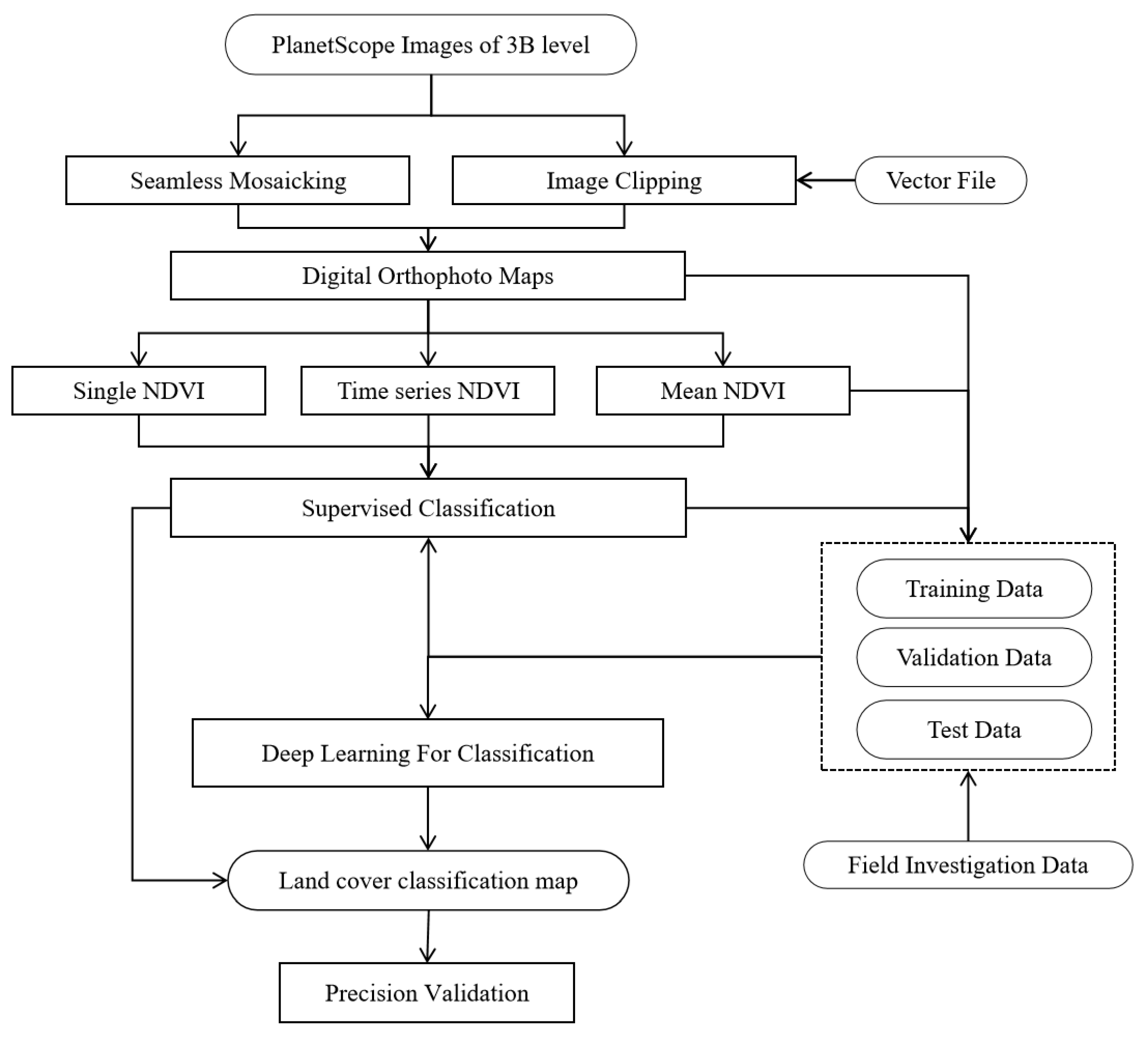
2.3.1. Method Framework

The process framework of this article is shown in Figure 2. The research is based on PlanetScope satellite remote-sensing images. After correction, seamless mosaic, clipping, resampling, and other preliminary data-processing operations on the original images, we build NDVI of the study area in 12 continuous months by using the red band and the near-infrared band. Then, through band-stacking of 12-month NDVI images, the data input in the subsequent classification can include the spatial position, spectral characteristics, and time series information. Image classification is realized by MLC and the deep-learning method in pixel-based direct classification. Finally, we analyzed the specific classification effect based on the overall classification results of the study area.

2.3.2. Data Preprocessing

Due to the large scope of the study area, the images of each month were captured by at least two dove satellites. So, we mosaicked multiple adjacent images. However, there are certain differences in the spectral information of images obtained by differently numbered satellites. In the process of seamless mosaic, color matching, boundary feathering, and other operations need to be carried out according to the overlapping area of adjacent images to achieve image uniformity. After obtaining the seamless mosaic image, the image should be clipped according to the boundary data of the study area. The premise of clipping was to unify the coordinate system of satellite images and boundary vectors. In this research, processing was in WGS84/UTM Zone 51 N coordinate system. Resampling was required when clipping was complete. We chose the nearest-pixel interpolation method to retain the original image information to the maximum extent. The size of mosaic images was 20,105 × 14,671 pixels.

NDVI data were produced based on the above images. The step of cloud removal was omitted because the cloud coverage of PlanetScope satellite images that were screened was low, as has been mentioned previously. The red band (590~670 nm) and the near-infrared band (780~860 nm) of these processed images were applied to generate NDVI images. After the raster processing of multi-band synthesis, all NDVI datasets were stacked into a time-series NDVI product with 12 bands in chronological order. Through band math from time-series NDVI, the mean NDVI data were generated as a reference. Additionally, the single NDVI in May 2022 was selected as data for subsequent comparison. Both will be the input data to compare with the time-series NDVI.

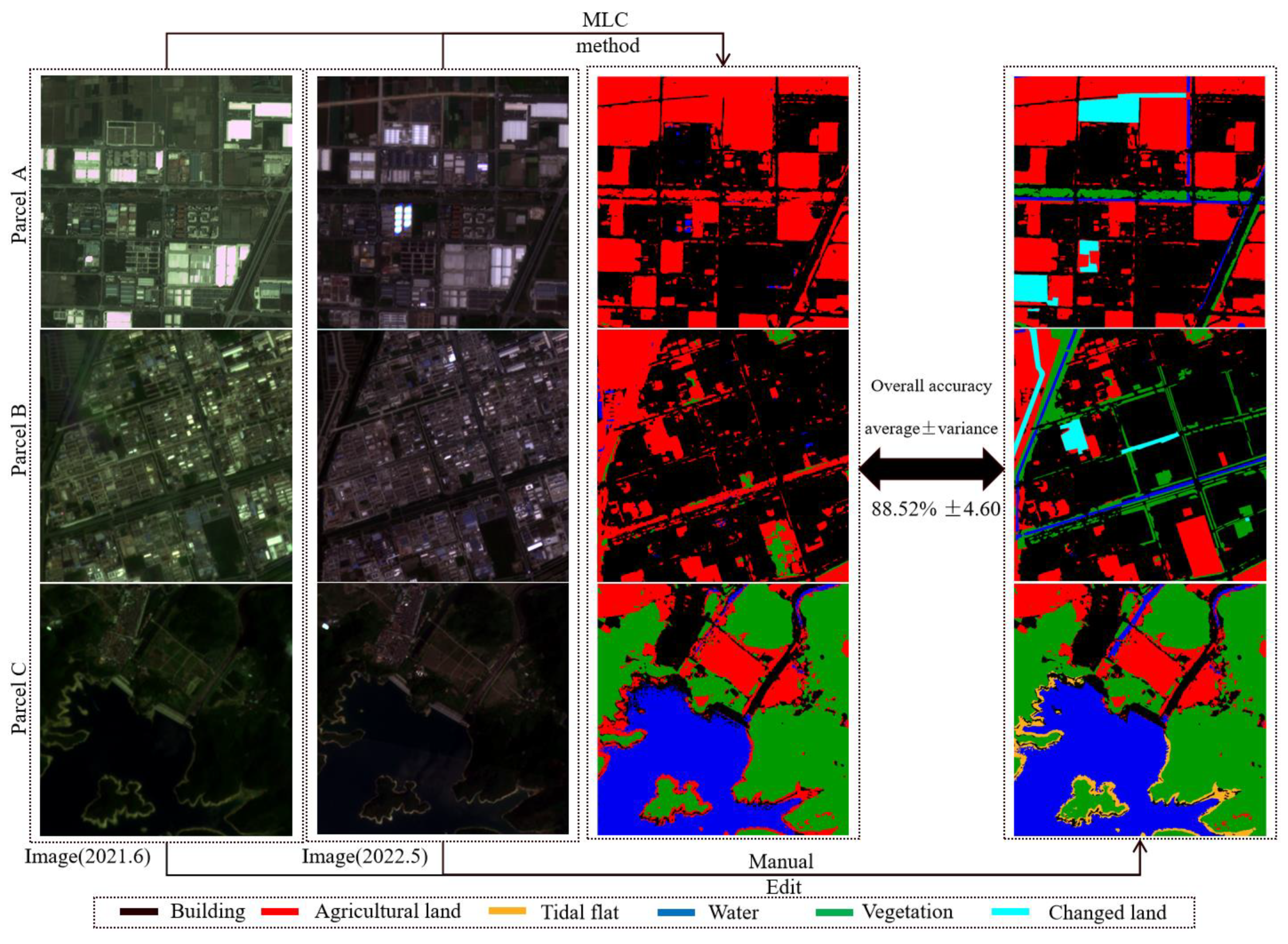
2.3.3. LULC Classification System and Method

Referring to the current land-use situation in the study area and the new version of the national standard classification of land-use status [37] organized and revised by the Ministry of land and resources of China in 2017, the land-use classes were divided into six categories, including five classes of unchanging land cover, namely, agricultural land, buildings, water, tidal flats, and vegetation. Additionally, one special class for land-change detection is called changed land. The specific detail of these six classes is described in

Table 2. Land use/land cover feature information table.

Class	Main features
Agricultural land	Cultivated land, paddy field, orchard, greenhouse, fishpond
Building	Road, city, village, industrial area
Vegetation	Forest, grassland
Water	River, lake, stream
Tidal flat	Beach, river beach, lake beach
Changed land	Areas where the type of features has changed

.

The classification strategy adopted is the pixel-based direct classification (DC) method. It is an effective method for processing time series data that such a scenario is not easy to model with expert knowledge but suitable for machine learning. Compared with the post-classification comparison method, it is more suited for LUCC because it can identify changes through only one stage without considering the error propagation from the wrong classification in each image [38]. The maximum-likelihood classification (MLC) based on statistical theory is a classification method used in the research; MLC is also called Bayesian classification. In two or more kinds of decisions of classification, this method uses a statistical method to set up a set of non-linear discriminant functions based on Bayesian Decision Criteria. Based on selecting training areas, assuming that each classification function corresponds to a normal distribution, the probability of the attribution of the area to be classified is calculated based on these statistics [39]. For this method, the results will be used for accuracy analysis on the one hand and will be used as the basis of deep-learning sample editing on the other hand.

Additionally, a deep-learning method of convolution neural network called U-Net was used in this study, which makes the input label images traverse the network with various weighting layers, including an input layer, an output layer, a convolution layer, and a pooling layer. The mapping rules between images and targets are established through various weight parameters. Many studies have confirmed the value and accuracy advantage of U-Net in the field of remote sensing change detection compared with traditional machine-learning classifiers such as Support Vector Machine (SVM) and Random Trees (RF) [40,41,42]. The U-Net model is a typical encoder–decoder architecture as an improvement and extension of FCN; its structure enables it to capture multiple features in the image context, which is advantageous for pixel-based DC method. It uses features spliced together in the channel size to form thicker features that are helpful for the analysis of time-series information. Meanwhile, U-Net can be trained from small datasets while ensuring reasonable segmentation accuracy. This is beneficial for change detection because there are relatively few training samples compared with other types of samples in study area [43,44,45]. Taking an image with 464 × 464 pixels containing 12 bands as an input example, the specific architecture is divided into 27 convolution layers (Figure 3). As shown in it, the shrinking network in the left half of the figure consists of five levels. Each level uses 3 × 3 convolution layer twice and 2 × 2 maximum pooling for downsampling. The expansion network structure of the right part is opposite, but the procedure is similar. Cross-entropy was used as the loss function in our network. For training the U-Net model of time series NDVI data, to optimize the results of image classification, multiple model parameters are continuously optimized and adjusted through randomized parameter training. Finally, the optimal model is selected according to the classification effect. A total of 555 images with 464 × 464 pixels in total were set as the input data, of which 80% were training data and 20% were testing data. In addition, image scaling and rotation were used to expand the samples.

We selected representative land-cover samples as the training area for MLC according to PlanetScope images, time series NDVI, and field survey data. According to the classification result of MLC, the training data for deep learning was generated. To illustrate the efficiency of editing MLC results, three 800 × 800-pixel areas were selected to verify the feasibility of obtaining samples for deep learning on the MLC results. We used confusion matrix to compare the results of the MLC method with direct visual interpretation. The comparative statistics of the three plots showed that the MLC results have a high similarity with the manually edited samples (Figure 4). The average overall pixel accuracy (±variance) between them reaches 88.52% (±4.60%). This means that sample editing based on MLC results is efficient and can provide a reference. The agricultural land in areas other than greenhouses, fishponds, and paddy fields, as well as other places such as water in main river and vegetation in the mountain, also have excellent classification accuracy that greatly reduces the workload of sample editing.

2.3.4. Evaluation Metrics and Materials

Confusion matrix analysis is the most commonly used method in the evaluation of image-classification accuracy. Statistical analysis of the matrix with the ground-truth type and the classification result can obtain an important classification accuracy evaluation index. True positive (TP), true negative (TP), false positive (FP), and false negative (FN) are four basic elements of the confusion matrix. They represent states corresponding to the classification results and ground truth. Overall accuracy (OA), recall, precision, F1-score, and Kappa coefficient are derived from the above four basic elements, and they are selected to evaluate the performance of the classification methodology [46,47]. Their specific formula is as follows:

$$\mathrm{OA}=\frac{\mathrm{TP}+\mathrm{TN}}{\mathrm{TP}+\mathrm{TN}+\mathrm{FP}+\mathrm{FN}}$$

(1)

$$\mathrm{Recall}=\frac{\mathrm{TP}}{\mathrm{TP}+\mathrm{FN}}$$

(2)

$$\mathrm{Precision}=\frac{\mathrm{TP}}{\mathrm{TP}+\mathrm{FP}}$$

(3)

$$\mathrm{F}1-\mathrm{score}=2\times \frac{\mathrm{Precision}\times \mathrm{Recall}}{\mathrm{Precision}+\mathrm{Recall}}$$

(4)

$$\mathrm{Kappa}=\frac{\mathrm{OA}-{\mathrm{P}}_{\mathrm{e}}}{1-{\mathrm{P}}_{\mathrm{e}}}$$

(5)

$${\mathrm{P}}_{\mathrm{e}}=\frac{{\mathrm{a}}_1\times {\mathrm{b}}_1+{\mathrm{a}}_2\times {\mathrm{b}}_2+\dots +{\mathrm{a}}_{\mathrm{n}}\times {\mathrm{b}}_{\mathrm{n}}}{\mathrm{N}\ast \mathrm{N}}$$

(6)

In the above equation,${ \mathrm{a}}_1$, ${\mathrm{a}}_2$, and ${\mathrm{a}}_{\mathrm{n}}$ represent the pixel number of real samples of each type. ${\mathrm{b}}_1$, ${\mathrm{b}}_2$, and ${\mathrm{b}}_{\mathrm{n}}$ represent the pixel number of samples of each type predicted. $\mathrm{n}$ represents the total number of land-cover types. $\mathrm{N}$ represents the total number of pixels in each sample.

Two forms of validation samples were selected for confusion matrix analysis. One was a ground-truth classification raster used to check five land covers without sample plots of changed land, and the other was ground truth points of interest that included changed land. The first sample data are 15 areas of 612 × 580 pixels. The area proportions of agricultural land, vegetation, water, buildings, and tidal flats are 43.5%, 16.9%, 12.8%, 26.6%, and 0.2%, respectively, in these data (Figure 5). These data were selected by referring to the satellite images and NDVI images, mainly used for robustness test.

The other validation samples are 902 typical points that were selected according to the field survey. The number of sample points for agricultural land, vegetation, water, buildings, tidal flats, and changed land are 230, 137, 196, 161, 53, and 125, respectively.

3. Results

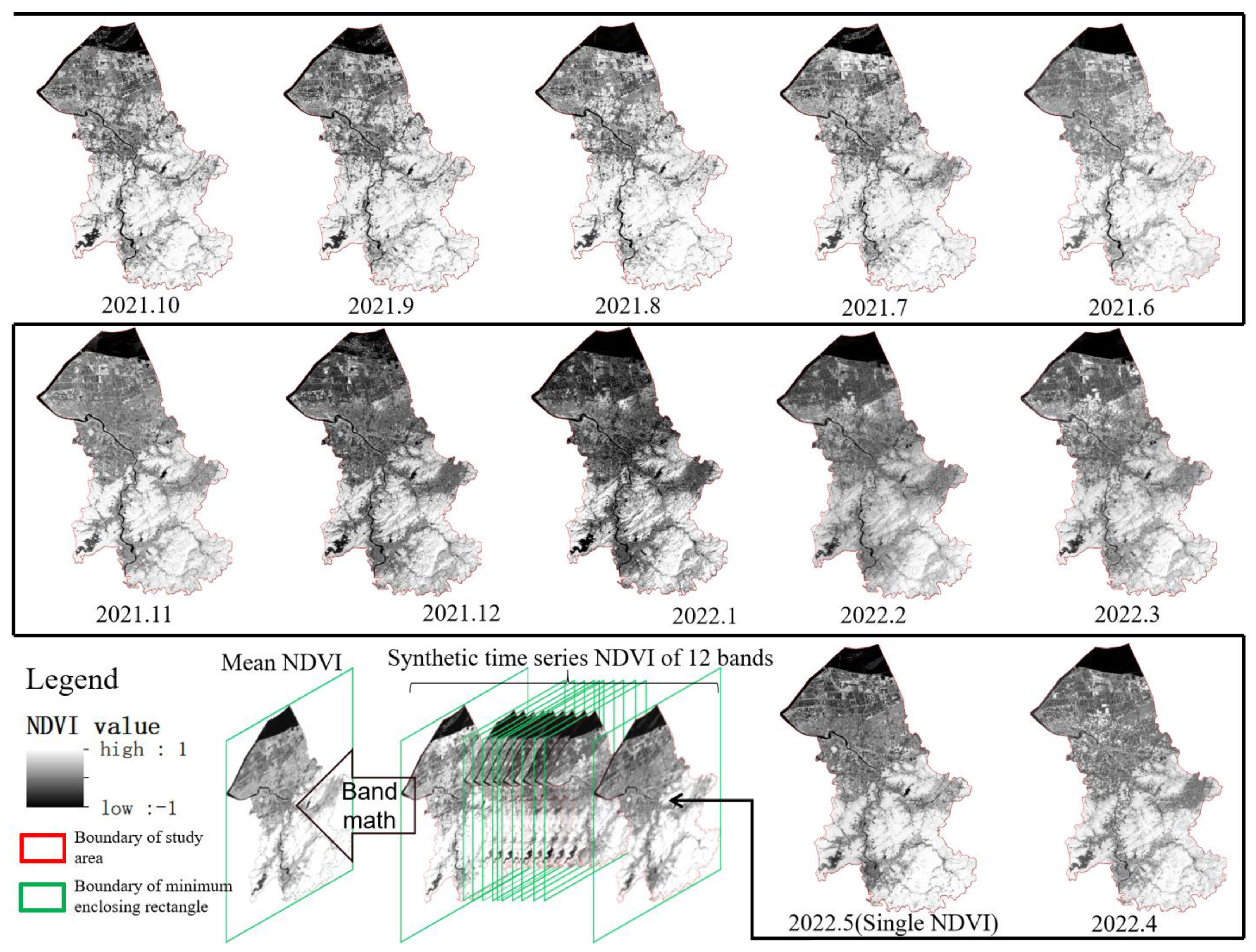
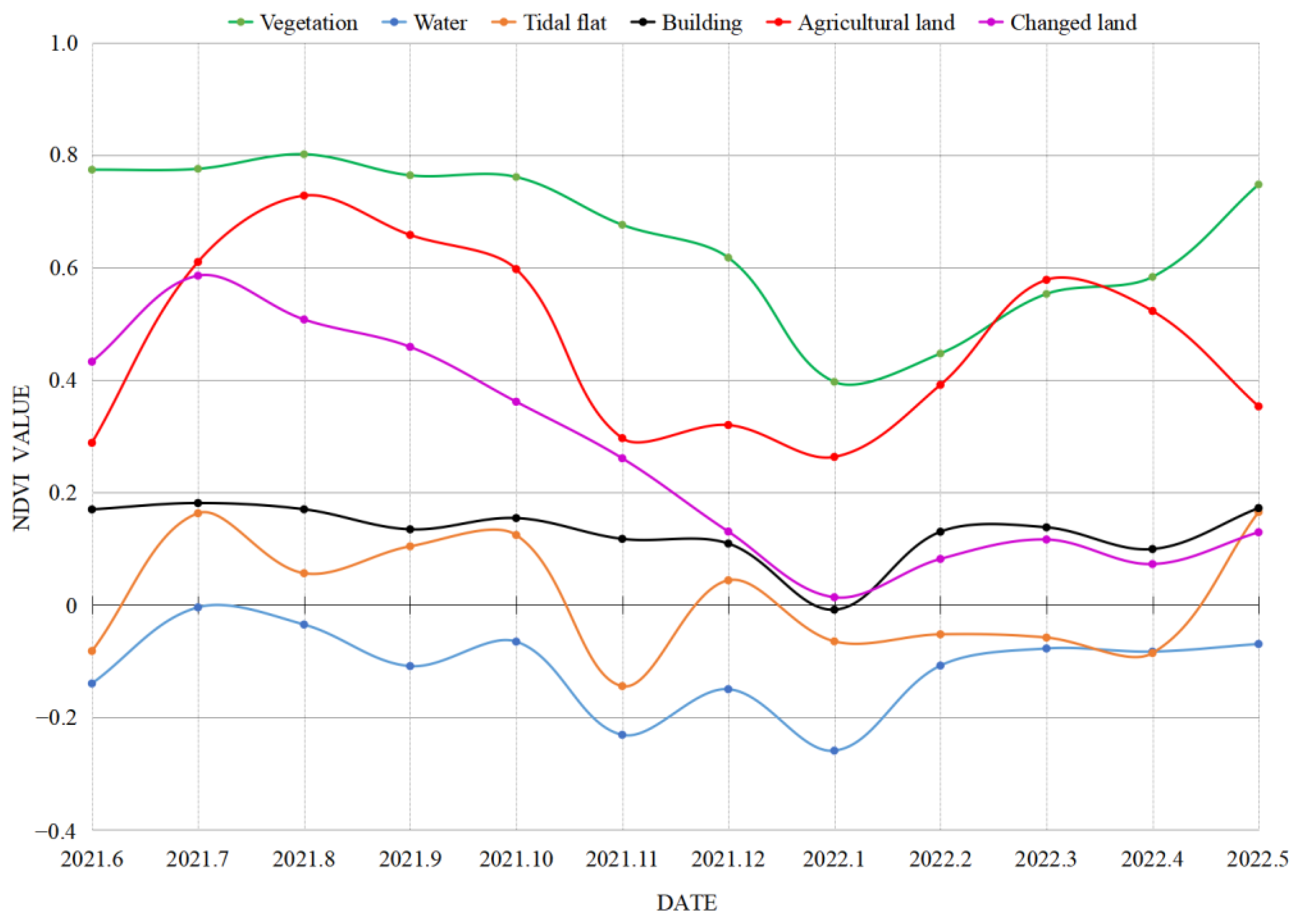
3.1. Time-Series NDVI Image Composition and Sample Labeling

The time-series NDVI image was obtained by processing the monthly multispectral images of the original PlanetScope products. From the monthly results (Figure 6), it can be found that the overall timing NDVI not only has a high spatial resolution but also has less noise, such as clouds, fog, and aerosols. All these index data were finally stacked into an annual multi-band image; every pixel contains one year’s NDVI information value. The mean NDVI was obtained by applying the average algorithm on the product.

A total of 10 typical land-cover points of ground truth from agricultural land, buildings, water, vegetation, tidal flats, and changed land (all changed land selected were from agricultural land converted to buildings) were selected to build the value spectral for confirming whether their value ranges are different. The point data values of each land-use type were averaged. Finally, the annual NDVI value curves of typical features were obtained. In the NDVI value curve (Figure 7), there is a large degree of separation between time-series value curves for various types of land cover. The NDVI value of water roughly fluctuates between 0 and −0.3. The value of buildings is stable between 0 and 0.2. Tidal flats are just between the two, but the fluctuation is slightly larger. In a year, the NDVI values of these three kinds of features change slightly, while the changes in vegetation and agricultural land are relatively large. As Shangyu district has a subtropical monsoon climate, the rice has the phenological characteristics of double-cropping in one season, and the harvest period is around June and October, which leads to two troughs in the NDVI curve. The NDVI value of vegetation is the highest in most cases and decreases in winter, which also conforms to the vegetation growth dynamics. The average NDVI of the sample points from agricultural land to buildings indicates that the two types of surface features changed in a few months. The consumption date of ground feature type transformation can also be estimated roughly by using the spectral curve. For example, the spectral curve of changed land in the figure is different from other features between July and December, so it can be regarded as a transition time of its change. These situations show that the use of annual time-series NDVI is valuable for surface-feature classification.

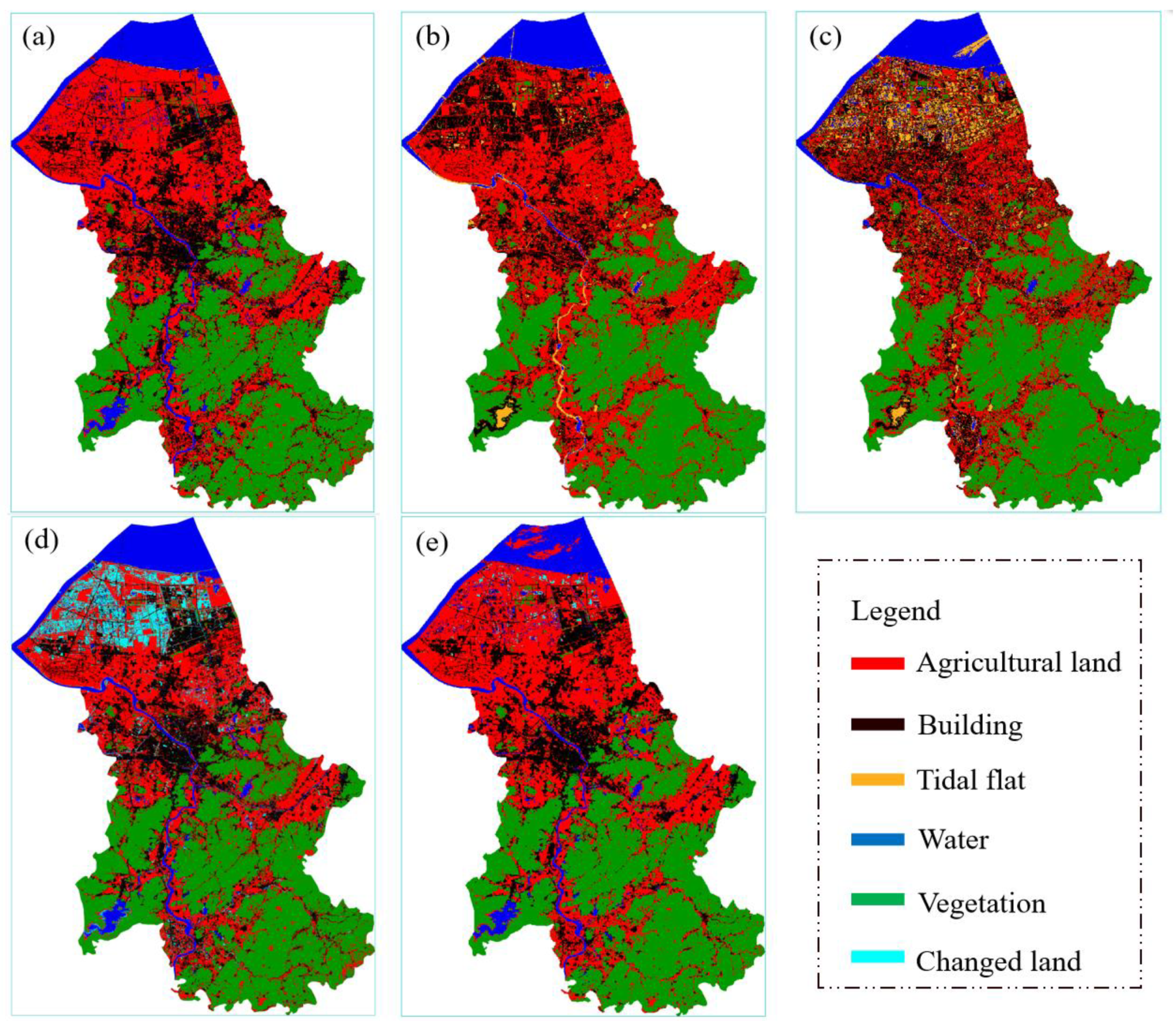
3.2. Classification Results and LUCC Statistics

The U-Net model used in this study experienced 400 epochs. The metrics of model training show that overall accuracy and loss value on training and testing data converge to above 0.97 and below 0.04, respectively. The training indicators are finally obtained through randomization parameter training. Patches per epoch and patches per batch were set to 300 and 1. The patch sample rate was 16, and the value of class weight used to highlight feature pixels at the beginning of training was set between 0.58 and 2.55. Loss weight was set to 0.46 for highlighting feature pixels when checking training effects.

Figure 8 presents all the classification results based on NDVI datasets. In this figure, (a), (b), and (c) represent MLC classification results of five land-cover types except changed land based on time series NDVI, mean NDVI, and single NDVI, respectively. The classification images from single NDVI and mean NDVI have many areas of confusing classification. The difference in the classification results of the main urban area in the north of Shangyu is particularly obvious. In these areas, many agricultural lands are wrongly identified as buildings in the mean NDVI, while most of them are classified as tidal flats in the single NDVI result. This phenomenon is largely due to the lack of temporal details, resulting in less information available for classification methods. For LUCC detection, (d) and (e) are the classification images of all six land-cover types based on time-series NDVI processed by MLC and U-Net, respectively. Additionally, the main difference is that a lot of agricultural land is misclassified as changed land in MLC. This is consistent with the statistics of the results (Figure 9).

In the statistics, the area of changed land is up to 89.87 square kilometers, accounting for 6.4% of Shangyu according to MLC results. It is too sensitive to change information extraction, especially in a farmland area. The statistical area of changed land in U-Net is fairer. According to the regional overview issued by the government of the study area in 2022, the area of vegetation cover in Shangyu district is 538.54 square kilometers (other land-use types are not indicated or do not match). The difference is only 13.3 square kilometers (2.5% of the actual area), which illustrates that the method based on time-series NDVI and U-Net in vegetation cover extraction is very effective.

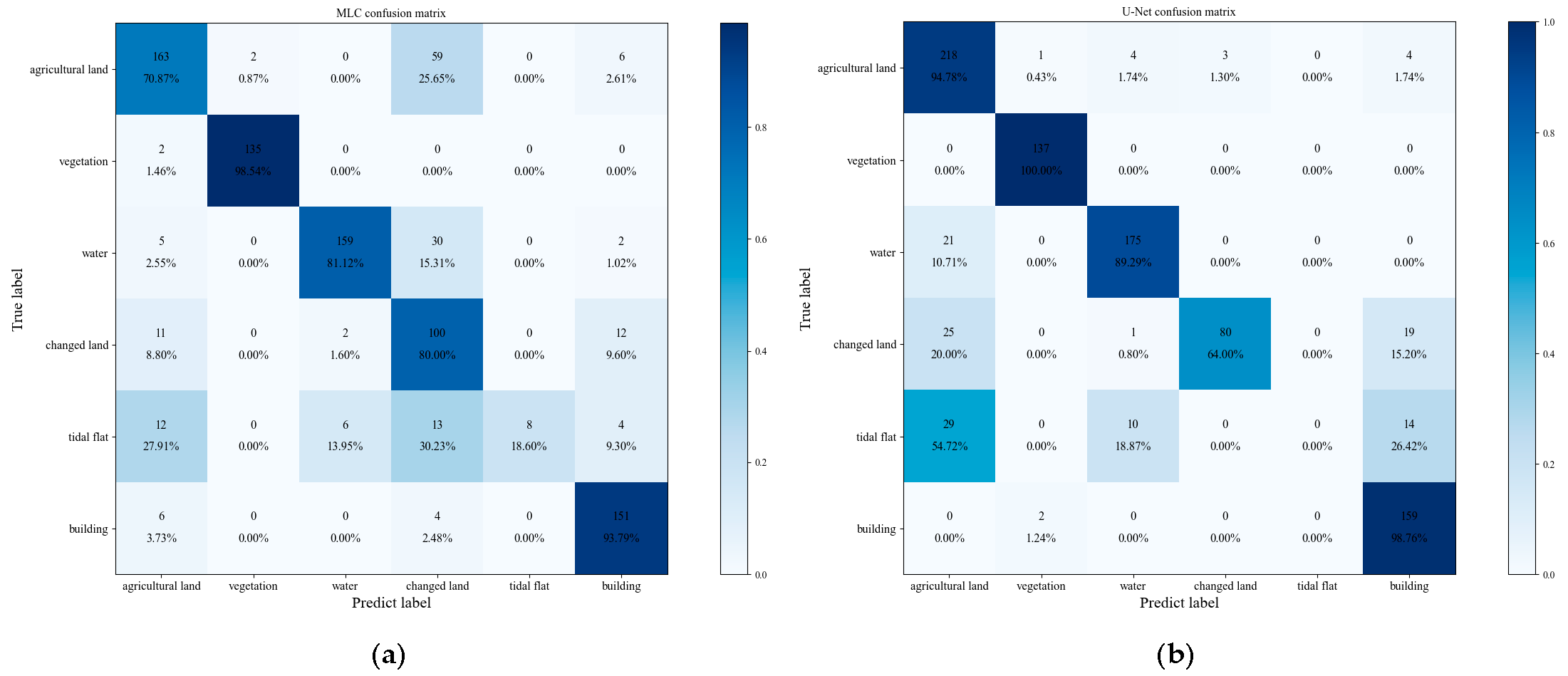
3.3. Confusion Matrix Analysis

According to the validation samples of raster data, which have been described before,

Table 3. Accuracy evaluation of confusion matrix.

Data	Method	Kappa	Overall Accuracy	Class	Recall	Precision	F1-Score
Single NDVI	MLC	0.36	52.32	Agricultural land	46.62	61.46	0.53
				Vegetation	56.79	77.28	0.65
				Water	62.12	86.67	0.72
				Buildings	54.15	45.91	0.50
				Tidal flats	39.65	0.51	0.01
Mean NDVI	MLC	0.45	62.15	Agricultural land	67.31	65.87	0.67
				Vegetation	48.16	91.60	0.63
				Water	44.84	99.25	0.62
				Buildings	71.01	52.11	0.60
				Tidal flats	52.15	2.02	0.04
Time-series NDVI	MLC	0.71	80.40	Agricultural land	85.98	77.11	0.81
				Vegetation	56.49	90.98	0.70
				Water	71.73	89.92	0.80
				Buildings	91.00	78.86	0.84
				Tidal flats	34.64	64.44	0.45
	MLC	0.59	69.65	Agricultural land	62.65	78.15	0.70
				Vegetation	56.50	90.97	0.70
				Water	68.84	95.02	0.80
				Buildings	90.10	80.35	0.85
				Tidal flats	34.89	64.50	0.45
				Changed land *	—
	U-Net	0.68	78.05	Agricultural land	84.23	75.04	0.79
				Vegetation	54.34	86.87	0.67
				Water	74.54	88.35	0.81
				Buildings	85.29	79.21	0.82
				Tidal flats	0.00	0.00	0.00
				Changed land *	—

* Indicates that these data lack samples in the ground truth. However, this class exists in the result of the classifier, which causes the denominator to be 0 during calculation and leads to meaningless data.

presents the confusion matrix results of each classification strategy. It shows that time-series NDVI is better for LULC classification than other types of NDVI data, not only in the overall accuracy but also in any class of land cover. Because the verification data has no intersection with the U-Net training or testing data, the information of these parcels has never been exposed to network training that can use them to test the robustness of the method. The accuracy results illustrate that the robustness of U-Net is better than MLC. In addition, after adding the sample of changed land in MLC, there are a lot of areas incorrectly identified as changed land that appear in these validation samples, which leads to a decrease in accuracy. A total of 61,633 pixels, which only account for 1.16% of the total, were classified as changed land by the U-Net classifier, while the MLC was up to 818,515, which accounts for 15.43% of the total. Various precision indexes of five and six classification types based on MLC also show that the expansion of the classification system will lead to a decline in the overall accuracy.

When using point validation data, the overall accuracy of MLC and U-Net is 79.38% and 85.26%, respectively, in the confusion matrix results (Figure 10a,b). This also proves that the U-Net method has higher precision than the MLC method. For changed land, although TP accounts for more than U-Net in the MLC method, the problem of extracting too much changed land still exists. The calculated F1-scores of MLC and U-Net are 0.77 and 0.66, respectively. It is considered that U-Net is more reasonable for the classification of changed land. One problem with U-net is that the classification effect of small samples, such as tidal flats (training sample pixels account for less than 0.1% of the total input images), is poor.

4. Discussion

4.1. Comparison of Classification Accuracy

When MLC was used for supervised classification, the accuracy of classification results obtained from different types of NDVI datasets varied greatly. Using raster validation samples for accuracy evaluation can reflect many problems. The overall accuracy of single-scene NDVI data was 52.32%, and the Kappa coefficient was 0.36. The classification effect was not good due to the lack of time-series information and the multiple values of the same type of land cover in a single image, resulting in excessive misclassification. Among them, the classification effect of Water was the best, with an F1-score of 0.72. Due to the asymmetry between actual ground truth and input samples that is mainly caused by the low area ratio and the large spectral difference, the classification effect of tidal flats was the worst, with an F1-score of only 0.01. Considering that the vegetation cover varies greatly in different periods, the mean NDVI of 12 months was used as the classification basis. Compared with single-scene NDVI, the classification accuracy of the mean NDVI was significantly improved, with an overall accuracy of 62.15% and Kappa coefficient of 0.45. Among them, the F1-score of agricultural land was 0.67, followed by buildings, vegetation, and water, but there was significant room for improvement. In order to give full play to the vegetation-sensitive characteristics of NDVI and more accurately reflect the change in vegetation cover in a period of time, the 12-month time-series NDVI was used for supervised classification. The overall accuracy of this method is 80.40%, and the Kappa coefficient is 0.71. Among them, buildings and agricultural land have achieved great classification effects, and the classification effect of difficult-to-distinguish tidal flats has also been significantly improved.

In view of the advantages of time-series NDVI, this study carried out change detection based on it. The changed land was regarded as an independent sample type. MLC and U-Net were, respectively, used for classification. Due to the complexity and diversity of the variable land-cover classes and the difficulty of feature extraction, the overall accuracy of the MLC decreased to 69.65%, and there were a lot of “excessive” phenomena. However, the deep-learning method could retrieve deeper feature information so as to effectively distinguish the “Changed land” from other land classes, with a total accuracy of 78.05%.

4.2. Deficiency and Implication

There are still some problems in the application of deep-learning methods for LULC classification and LUCC detection based on time-series NDVI, which leads to the deviation of classification results. First, the annotation of deep learning samples consumes a lot of time and energy and is prone to errors, resulting in model deviation; second, there are geometric distortions in remote-sensing images of different periods, such as road deformation and house distortion. These geometric changes will be incorrectly classified as change areas; third, unstable objects can interfere with change detection, such as (1) moving aircraft and factory chimney emissions of gas, (2) agricultural greenhouses that vary significantly with the seasons, and (3) the influence of a partial sun angle and cloud shadows. Fourth, the complexity of ground feature types in urban areas can reduce the accuracy of classification. The characteristics of land cover, such as the unbalanced proportion of each category and the fragmentation of land-cover patches, make it difficult to identify and extract features. Three kinds of problems were found in the classification results: (1) the extraction effect of tidal flats with a small and variable area ratio was not ideal; (2) in the north, agricultural land and towns are intersected and scattered, while in the south, woodlands are interspersed with some small areas of agricultural land. The boundary contour of different categories is not clear enough, leading to classification errors; (3) a large area of northern water was misclassified as agricultural land, and some water was also found in the agricultural land classification. This is because there is a large area of fish ponds and paddy fields in this area. Although the semantics are different, the spectral characteristics are similar, which affects the classification of water and agricultural land.

In view of the problems in this experiment, the LULC classification method used in this article still has a lot of room for progress. First, it is necessary to optimize the model algorithm to reduce the workload of manual annotation as much as possible while ensuring classification accuracy. Second, making full use of the contextual information in the image to improve the classification accuracy is the direction of efforts; third, the data sources used in this study are relatively simple. A good research direction might involve fully integrating the advantages of different data sources (e.g., DEM, radar images, and spatial–temporal big data) to improve classification accuracy.

5. Conclusions

In this article, we used the 2021–2022 time-series NDVI image that was generated from PlanetScope satellite images to obtain LUCC maps of the study area. PlanetScope satellite products have the advantages of high temporal and spatial resolution, which makes generated NDVI data have a good interpretation for classification. By comparing the classification accuracy of the MLC method, the evaluation metrics demonstrate that time-series NDVI is far better than single NDVI and mean NDVI as basic data for land-cover classification under complex environments. Meanwhile, editing samples based on MLC results can also be an efficient way to train a deep-learning model. The other method of LUCC detection is the U-Net image-segmentation model. Through confusion matrix analysis, it was found that U-Net is better than MLC and can improve the situation of excessive classification to changed land, which is significant in LUCC detection. However, the classification of small samples, such as tidal flats, needs to be improved.

The results show that the process framework is an efficient and reliable method for information extraction in LUCC. In the future, the application and research of the PlanetScope satellite data will continue to increase; the ability of the deep-learning model to be transferred to other regions also makes it preferred by remote-sensing application researchers.

References

1. Chu, X.L.; Lu, Z.; Wei, D.; Lei, G.P. Effects of land use/cover change (LUCC) on the spatiotemporal variability of precipitation and temperature in the Songnen Plain, China. J. Integr. Agric. 2022, 21, 235–248. [Google Scholar] [CrossRef]
2. Ul Din, S.; Mak, H.W.L. Retrieval of Land-Use/Land Cover Change (LUCC) Maps and Urban Expansion Dynamics of Hyderabad, Pakistan via Landsat Datasets and Support Vector Machine Framework. Remote Sens. 2021, 13, 3337. [Google Scholar] [CrossRef]
3. Vali, A.; Comai, S.; Matteucci, M. Deep Learning for Land Use and Land Cover Classification Based on Hyperspectral and Multispectral Earth Observation Data: A Review. Remote Sens. 2020, 12, 2495. [Google Scholar] [CrossRef]
4. Seydi, S.T.; Akhoondzadeh, M.; Amani, M.; Mahdavi, S. Wildfire Damage Assessment over Australia Using Sentinel-2 Imagery and MODIS Land Cover Product within the Google Earth Engine Cloud Platform. Remote Sens. 2021, 13, 220. [Google Scholar] [CrossRef]
5. Li, G.; Zhang, F.M.; Jing, Y.S.; Liu, Y.B.; Sun, G. Response of evapotranspiration to changes in land use and land cover and climate in China during 2001–2013. Sci. Total Environ. 2017, 596, 256–265. [Google Scholar] [CrossRef]
6. Souza, C.M.; Shimbo, J.Z.; Rosa, M.R.; Parente, L.L.; Alencar, A.A.; Rudorff, B.F.T.; Hasenack, H.; Matsumoto, M.; Ferreira, L.G.; Souza, P.W.M.; et al. Reconstructing Three Decades of Land Use and Land Cover Changes in Brazilian Biomes with Landsat Archive and Earth Engine. Remote Sens. 2020, 12, 2735. [Google Scholar] [CrossRef]
7. Sanchez-Espinosa, A.; Schroder, C. Land use and land cover mapping in wetlands one step closer to the ground: Sentinel-2 versus landsat 8. J. Environ. Manag. 2019, 247, 484–498. [Google Scholar] [CrossRef]
8. Cai, G.Y.; Ren, H.Q.; Yang, L.Z.; Zhang, N.; Du, M.Y.; Wu, C.S. Detailed Urban Land Use Land Cover Classification at the Metropolitan Scale Using a Three-Layer Classification Scheme. Sensors 2019, 19, 3120. [Google Scholar] [CrossRef] [Green Version]
9. Fu, Y.Y.; Ye, Z.R.; Deng, J.S.; Zheng, X.Y.; Huang, Y.B.; Yang, W.; Wang, Y.H.; Wang, K. Finer Resolution Mapping of Marine Aquaculture Areas Using WorldView-2 Imagery and a Hierarchical Cascade Convolutional Neural Network. Remote Sens. 2019, 11, 1678. [Google Scholar] [CrossRef] [Green Version]
10. Huang, Y.H.; Wu, C.B.; Yang, H.J.; Zhu, H.T.; Chen, M.X.; Yang, J. An Improved Deep Learning Approach for Retrieving Outfalls Into Rivers From UAS Imagery. IEEE Trans. Geosci. Remote Sens. 2022, 60, 14. [Google Scholar] [CrossRef]
11. Aguiler, M.A.Z. Classication of land-cover through machine learning algorithms for fusion of Sentinel-2a and planetscope imagery. In Proceedings of the IEEE Latin American GRSS and ISPRS Remote Sensing Conference (LAGIRS), Santiago, Chile, 21–26 March 2020; pp. 246–253. [Google Scholar]
12. Francini, S.; McRoberts, R.E.; Giannetti, F.; Mencucci, M.; Marchetti, M.; Mugnozza, G.S.; Chirici, G. Near-real time forest change detection using PlanetScope imagery. Eur. J. Remote Sens. 2020, 53, 233–244. [Google Scholar] [CrossRef]
13. Gabr, B.; Ahmed, M.; Marmoush, Y. PlanetScope and Landsat 8 Imageries for Bathymetry Mapping. J. Mar. Sci. Eng. 2020, 8, 143. [Google Scholar] [CrossRef] [Green Version]
14. Cheng, Y.; Vrieling, A.; Fava, F.; Meroni, M.; Marshall, M.; Gachoki, S. Phenology of short vegetation cycles in a Kenyan rangeland from PlanetScope and Sentinel-2. Remote Sens. Environ. 2020, 248, 20. [Google Scholar] [CrossRef]
15. Yan, J.N.; Wang, L.Z.; Song, W.J.; Chen, Y.L.; Chen, X.D.; Deng, Z. A time-series classification approach based on change detection for rapid land cover mapping. ISPRS-J. Photogramm. Remote Sens. 2019, 158, 249–262. [Google Scholar] [CrossRef]
16. Wei, B.C.; Xie, Y.W.; Wang, X.Y.; Jiao, J.Z.; He, S.J.; Bie, Q.; Jia, X.; Xue, X.Y.; Duan, H.M. Land cover mapping based on time-series MODIS-NDVI using a dynamic time warping approach: A casestudy of the agricultural pastoral ecotone of northern China. Land Degrad. Dev. 2020, 31, 1050–1068. [Google Scholar] [CrossRef]
17. Chu, H.S.; Venevsky, S.; Wu, C.; Wang, M.H. NDVI-based vegetation dynamics and its response to climate changes at Amur-Heilongjiang River Basin from 1982 to 2015. Sci. Total Environ. 2019, 650, 2051–2062. [Google Scholar] [CrossRef]
18. Gao, W.D.; Zheng, C.; Liu, X.H.; Lu, Y.D.; Chen, Y.F.; Wei, Y.; Ma, Y.D. NDVI-based vegetation dynamics and their responses to climate change and human activities from 1982 to 2020: A case study in the Mu Us Sandy Land, China. Ecol. Indic. 2022, 137, 14. [Google Scholar] [CrossRef]
19. Matongera, T.N.; Mutanga, O.; Sibanda, M.; Odindi, J. Estimating and Monitoring Land Surface Phenology in Rangelands: A Review of Progress and Challenges. Remote Sens. 2021, 13, 2060. [Google Scholar] [CrossRef]
20. Zhou, J.X.; Chen, J.; Chen, X.H.; Zhu, X.L.; Qiu, Y.A.; Song, H.H.; Rao, Y.H.; Zhang, C.S.; Cao, X.; Cui, X.H. Sensitivity of six typical spatiotemporal fusion methods to different influential factors: A comparative study for a normalized difference vegetation index time series reconstruction. Remote Sens. Environ. 2021, 252, 21. [Google Scholar] [CrossRef]
21. Kong, F.J.; Li, X.B.; Wang, H.; Xie, D.F.; Li, X.; Bai, Y.X. Land Cover Classification Based on Fused Data from GF-1 and MODIS NDVI Time Series. Remote Sens. 2016, 8, 741. [Google Scholar] [CrossRef]
22. Jia, K.; Liang, S.L.; Wei, X.Q.; Yao, Y.J.; Su, Y.R.; Jiang, B.; Wang, X.X. Land Cover Classification of Landsat Data with Phenological Features Extracted from Time Series MODIS NDVI Data. Remote Sens. 2014, 6, 11518–11532. [Google Scholar] [CrossRef] [Green Version]
23. Ashourloo, D.; Shahrabi, H.S.; Azadbakht, M.; Rad, A.M.; Aghighi, H.; Radiom, S. A novel method for automatic potato mapping using time series of Sentinel-2 images. Comput. Electron. Agric. 2020, 175, 13. [Google Scholar] [CrossRef]
24. Baeza, S.; Paruelo, J.M. Land Use/Land Cover Change (2000-2014) in the Rio de la Plata Grasslands: An Analysis Based on MODIS NDVI Time Series. Remote Sens. 2020, 12, 381. [Google Scholar] [CrossRef] [Green Version]
25. Phalke, A.R.; Ozdogan, M.; Thenkabail, P.S.; Erickson, T.; Gorelick, N.; Yadav, K.; Congalton, R.G. Mapping croplands of Europe, Middle East, Russia, and Central Asia using Landsat, Random Forest, and Google Earth Engine. ISPRS-J. Photogramm. Remote Sens. 2020, 167, 104–122. [Google Scholar] [CrossRef]
26. Tassi, A.; Vizzari, M. Object-Oriented LULC Classification in Google Earth Engine Combining SNIC, GLCM, and Machine Learning Algorithms. Remote Sens. 2020, 12, 3776. [Google Scholar] [CrossRef]
27. Talukdar, S.; Singha, P.; Mahato, S.; Shahfahad; Pal, S.; Liou, Y.A.; Rahman, A. Land-Use Land-Cover Classification by Machine Learning Classifiers for Satellite Observations-A Review. Remote Sens. 2020, 12, 1135. [Google Scholar] [CrossRef] [Green Version]
28. Ghayour, L.; Neshat, A.; Paryani, S.; Shahabi, H.; Shirzadi, A.; Chen, W.; Al-Ansari, N.; Geertsema, M.; Amiri, M.P.; Gholamnia, M.; et al. Performance Evaluation of Sentinel-2 and Landsat 8 OLI Data for Land Cover/Use Classification Using a Comparison between Machine Learning Algorithms. Remote Sens. 2021, 13, 1349. [Google Scholar] [CrossRef]
29. Schneider, A. Monitoring land cover change in urban and pen-urban areas using dense time stacks of Landsat satellite data and a data mining approach. Remote Sens. Environ. 2012, 124, 689–704. [Google Scholar] [CrossRef]
30. Wang, X.; Liu, S.C.; Du, P.J.; Liang, H.; Xia, J.S.; Li, Y.F. Object-Based Change Detection in Urban Areas from High Spatial Resolution Images Based on Multiple Features and Ensemble Learning. Remote Sens. 2018, 10, 276. [Google Scholar] [CrossRef] [Green Version]
31. Ma, L.; Liu, Y.; Zhang, X.L.; Ye, Y.X.; Yin, G.F.; Johnson, B.A. Deep learning in remote sensing applications: A meta-analysis and review. ISPRS-J. Photogramm. Remote Sens. 2019, 152, 166–177. [Google Scholar] [CrossRef]
32. Yuan, Q.Q.; Shen, H.F.; Li, T.W.; Li, Z.W.; Li, S.W.; Jiang, Y.; Xu, H.Z.; Tan, W.W.; Yang, Q.Q.; Wang, J.W.; et al. Deep learning in environmental remote sensing: Achievements and challenges. Remote Sens. Environ. 2020, 241, 24. [Google Scholar] [CrossRef]
33. Alhassan, V.; Henry, C.; Ramanna, S.; Storie, C. A deep learning framework for land-use/land-cover mapping and analysis using multispectral satellite imagery. Neural Comput. Appl. 2020, 32, 8529–8544. [Google Scholar] [CrossRef]
34. Solorzano, J.V.; Mas, J.F.; Gao, Y.; Gallardo-Cruz, J.A. Land Use Land Cover Classification with U-Net: Advantages of Combining Sentinel-1 and Sentinel-2 Imagery. Remote Sens. 2021, 13, 3600. [Google Scholar] [CrossRef]
35. Zhang, X.; Yang, G.X.; Xu, X.J.; Yao, X.; Zheng, H.B.; Zhu, Y.; Cao, W.X.; Cheng, T. An assessment of Planet satellite imagery for county-wide mapping of rice planting areas in Jiangsu Province, China with one-class classification approaches. Int. J. Remote Sens. 2021, 42, 7610–7635. [Google Scholar] [CrossRef]
36. Houborg, R.; McCabe, M.F. High-Resolution NDVI from Planet’s Constellation of Earth Observing Nano-Satellites: A New Data Source for Precision Agriculture. Remote Sens. 2016, 8, 768. [Google Scholar] [CrossRef] [Green Version]
37. GB/T 21010-201; Current Land Use Classification. China National Standardization Management Committee: Beijing, China, 2017; p. 16.
38. Tewkesbury, A.P.; Comber, A.J.; Tate, N.J.; Lamb, A.; Fisher, P.F. A critical synthesis of remotely sensed optical image change detection techniques. Remote Sens. Environ. 2015, 160, 1–14. [Google Scholar] [CrossRef] [Green Version]
39. Cabral, A.I.R.; Silva, S.; Silva, P.C.; Vanneschi, L.; Vasconcelos, M.J. Burned area estimations derived from Landsat ETM plus and OLI data: Comparing Genetic Programming with Maximum Likelihood and Classification and Regression Trees. ISPRS-J. Photogramm. Remote Sens. 2018, 142, 94–105. [Google Scholar] [CrossRef]
40. Kumar, M.S.; Jayagopal, P. Delineation of field boundary from multispectral satellite images through U-Net segmentation and template matching. Ecol. Inform. 2021, 64, 14. [Google Scholar] [CrossRef]
41. Zhang, J.; Xie, T.J.; Yang, C.H.; Song, H.B.; Jiang, Z.; Zhou, G.S.; Zhang, D.Y.; Feng, H.; Xie, J. Segmenting Purple Rapeseed Leaves in the Field from UAV RGB Imagery Using Deep Learning as an Auxiliary Means for Nitrogen Stress Detection. Remote Sens. 2020, 12, 1403. [Google Scholar] [CrossRef]
42. Morgan, G.R.; Wang, C.Z.; Li, Z.L.; Schill, S.R.; Morgan, D.R. Deep Learning of High-Resolution Aerial Imagery for Coastal Marsh Change Detection: A Comparative Study. ISPRS Int. J. Geo-Inf. 2022, 11, 100. [Google Scholar] [CrossRef]
43. Ronneberger, O.; Fischer, P.; Brox, T. U-Net: Convolutional Networks for Biomedical Image Segmentation. In Medical Image Computing and Computer-Assisted Intervention—MICCAI 2015; Springer International Publishing: Cham, Switzerland, 2015; pp. 234–241. [Google Scholar] [CrossRef] [Green Version]
44. Li, H.X.; Wang, C.Z.; Cui, Y.X.; Hodgson, M. Mapping salt marsh along coastal South Carolina using U-Net. ISPRS-J. Photogramm. Remote Sens. 2021, 179, 121–132. [Google Scholar] [CrossRef]
45. Wei, J.J.; Zhang, Y.H.; Wu, H.A.; Cui, B. An Efficient Change Detection for Large SAR Images Based on Modified U-Net Framework. Can. J. Remote Sens. 2020, 46, 272–294. [Google Scholar] [CrossRef]
46. Foody, G.M. Status of land cover classification accuracy assessment. Remote Sens. Environ. 2002, 80, 185–201. [Google Scholar] [CrossRef]
47. Maxwell, A.E.; Warner, T.A.; Guillen, L.A. Accuracy Assessment in Convolutional Neural Network-Based Deep Learning Remote Sensing Studies-Part 2: Recommendations and Best Practices. Remote Sens. 2021, 13, 2591. [Google Scholar] [CrossRef]
Figure 1. Schematic diagram of the study area, Shangyu district, Shaoxing City, Zhejiang Province, China (the digital orthophoto map is processed on 10 adjacent images obtained by PlanetScope satellite on 17 May 2022).
Water 14 03363 g001
Figure 2. Method framework of LUCC research based on NDVI from PlanetScope satellite images.
Water 14 03363 g002
Figure 3. U-Net network architecture processing diagram (with a 464 × 464 × 12 image as an example).
Water 14 03363 g003
Figure 4. Comparison between manually edited samples and MLC results of three grounds.
Water 14 03363 g004
Figure 5. Formation and composition of various classes at raster validation data.
Water 14 03363 g005
Figure 6. Annual NDVI images displayed by time series.
Water 14 03363 g006
Figure 7. Annual NDVI value curves (each curve represents the NDVI value of a typical feature, and each point in the curve represents the mean value of 10 typical features).
Water 14 03363 g007
Figure 8. Classification results of (a) MLC method without change detection based on time-series NDVI; (b) MLC method change detection based on mean NDVI; (c) MLC method change detection based on single NDVI; (d) MLC method including change detection based on time-series NDVI; (e) U-Net method including change detection based on time-series NDVI.
Water 14 03363 g008
Figure 9. Area statistics of each ground feature comparing MLC and U-Net.
Water 14 03363 g009
Figure 10. Confusion matrix results at 902-point validation data. (a) MLC confusion matrix. (b) U-Net confusion matrix.
Water 14 03363 g010