Effect of Static Magnetic Fields on the Composition of Marine Biofouling in Seawater Transportation Pipelines

Abstract

The use of seawater for mining purposes in Chile has progressively increased in recent years as fast as the interest on the negative effects of biofouling on the inner part of pipelines used to transport seawater. To prevent biofouling, chemical antifouling compounds are traditionally used, thus, causing negative environmental impacts. The aim of this research has, therefore, been to evaluate the efficiency of static magnetic fields (SMF) generators to mitigate the biofouling. Hence, experimental activities have been conducted on high density polyethylene (HDPE) pipes equipped with neodymium magnets during two experimental periods in the year of 2019, i.e., autumn–winter (A–W) and spring–summer (S–S), and under two types of SMF, i.e., continuous-type (PCS) and pulse-type (PPS). Physicochemical parameters and cell viability of microorganisms composing the biofilm were investigated. Metagenomic analyses on biofilm were conducted as well. The results showed that the cell viability was the highest, i.e., 757,780 cells/cm², during S–S and the lowest, i.e., 349,151 cells/cm², in A–W, both under PCS. In S–S, as well as A–W, biofilm was characterized for the most abundant eukaryotic operational taxonomic units (OTUs) under PPS conditions. The presence of OTUs, such as Articiflavibacter spp., Chaetonotida spp. and Desmodorida spp., was observed only from SMF tests.

1. Introduction

As a consequence of water scarcity that is currently affecting Chile, as well as many other countries in the world, the use of seawater as a water resource for industrial processes, e.g., mining, has progressively increased in the last decades [1]. Usually mining areas are far from the coastline, which implies the transportation of seawater for long distance (longer than 100 km) is performed by pipelines [2,3]. Marine microorganisms and high salinity in seawater are responsible for the formation of marine life-based biofouling on the inner part of the pipelines, thus, decreasing notably the transport efficiency and, consequently, the industrial systems performance, as well as causing the materials’ property decay and, consequently the shortening of their service life [4]. A practical and traditional approach to prevent the biofouling is the addition of chemical antifouling compounds to seawater, but this method is not free of environmental concerns [5].

The richness in nutrients and the high biodiversity that characterize Chile’s marine environment [6] are the key factors for a rapid biofouling formation on the surface of all types of materials exposed to seawater [5,6,7]. Biofouling is composed of biofilms, i.e., a community of microorganisms attached to a solid surface; [8,9] described a high microbial richness (with more than 7300 species revealed from 101 biofilm metagenomes), including sessile bacteria, microalgae including diatoms, microscopic fungi, heterotrophic flagellates and sessile ciliates (heterotrophic protists) [9,10]. In general, it has been described that biofouling represents a resistant structure that is composed of layers of biofilm, whose structure is the result of the effects produced by several external agents of climatic or anthropogenic origin [8], better known with the generic name of disturbances. Disturbances are generally divided in two categories: pulse-type and continuous-type disturbances. A pulse-type disturbance causes a short-term impact that alters the density of communities [11], e.g., natural disturbances are commonly pulse-type disturbances and are followed by a reorganization phase. Conversely, a continuous-type disturbance causes a long-term impact, sufficient to keep the equilibrium system perturbed for a long time [11,12,13].

Static magnetic field (SMF) represents a sort of disturbance that can affect microbial communities. An SMF is a ubiquitous environmental factor for all living organisms during the evolutionary process. Various studies have proven that bacteria, algae, invertebrates, plants, birds, mice and even humans are capable of detecting the Earth’s magnetic field for orientation in navigation and migration, in case of escape and nest building [14]. Continuous and pulse exposures of organisms to SMFs of higher intensity than the geomagnetic field has been studied along the years. Several hypotheses have been proposed to explain the interactions between SMFs and biological systems, including magnetic induction, magnetite hypothesis and free radical pair mechanism [15]. Nevertheless, the exact mechanisms that govern the effect of SMFs on living systems are largely unknown, and there is no single theory that can comprehensively explain the interaction between magnetic field and organisms.

Some studies have described the effect of SMF on microorganisms [16] through morphological studies using a transmission electron microscope (TEM) and have detected damages to the bacterial cell wall caused by exposure to SMF. In fungi, a mycelial growth inhibition has been observed as a response to 300 mT SMF coupled with morphological and biochemical changes [17]. The effects of SMF on microorganisms not only depend on the species and their morphology but also on the characteristics of the culture medium where the magnetic field is active [18]. SMFs in aqueous systems produce changes in the environment properties, thus, modifying the kinetics of physicochemical processes and, consequently, the performance of technological and biological systems that rely on such processes. These variations are generally small but are sufficient to significantly affect biological and industrial systems [19].

Despite the impacts of SMFs on unicellular microorganisms, there are very few studies describing the effects of SMFs on complex micro communities, such as a marine biofilm, where interspecific biotic, as well abiotic interactions occur among different species of microorganisms and the surrounding environment. Some studies have shown that SMF has an impact on biofilms, however, most of these studies have been performed with single species and in the laboratory. For example, it was determined that in the presence of 200 mT, SMF significantly enhanced biofilm formation and swarming in Pseudomonas aeruginosa [20]. In exoelectrogenic biofilms of Geobacteraceae, it was shown that the use of low-intensity magnetic field (105 and 150 mT) with short-term application increases biofilm conductivity [21], and Letuta and Tikhonova [22] demonstrated that Escherichia coli biofilms are stimulated in the presence of low-intensity SMF (20–35 mT). Therefore, the aim of this research has been to study the composition of the biofilm growing on the inner surface of pipelines, transporting seawater and the effects that the SMFs supplied as continuous- and pulse-type disturbance caused on it, thus, contributing knowledge that will be useful in the future for developing a new antifouling system with a low environmental impact.

2. Materials and Methods

2.1. Experimental Pipeline Transportation System

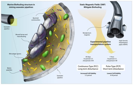
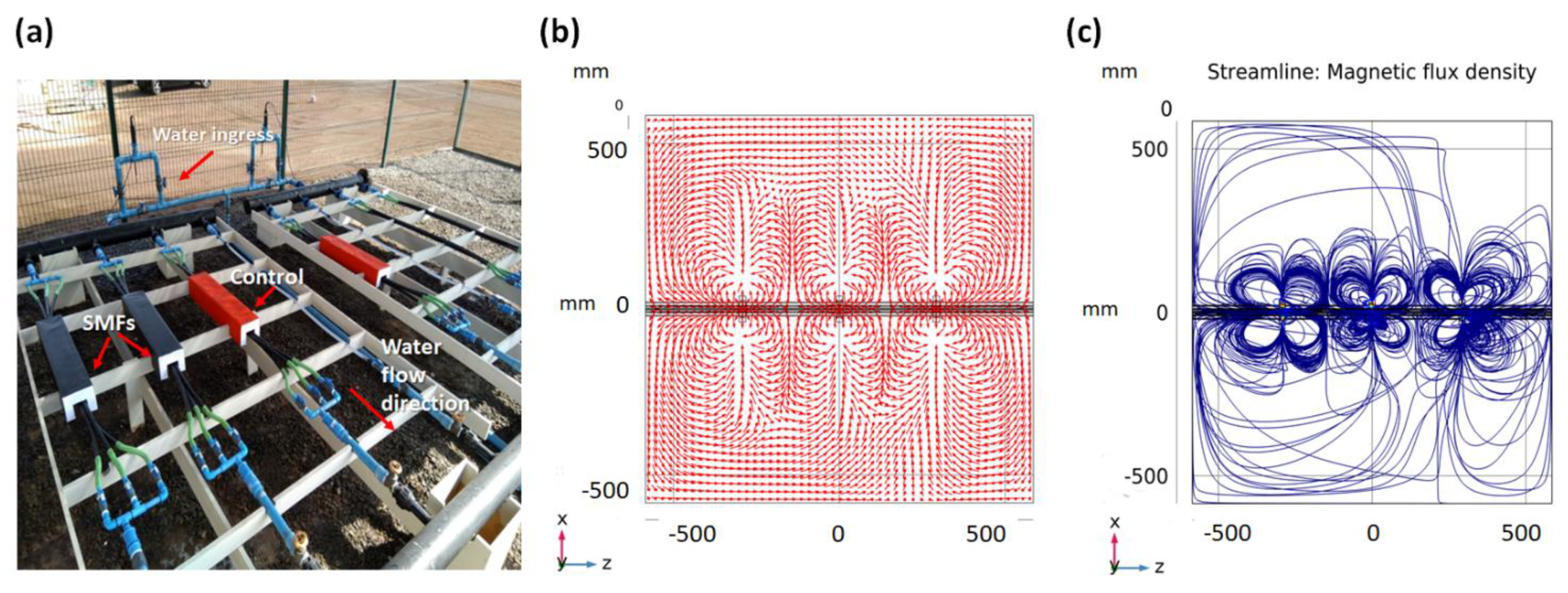
Eighteen high density polyethylene (HDPE) pipes with a diameter of 1.8 cm and a length of 120 cm were used to transport seawater. The pipeline transportation system was fed with raw seawater collected directly from San Jorge Bay in Antofagasta (latitude 23.70263° S, longitude 70.41984° O) and flowing through the pipeline system continuously and uninterruptedly for 60 observation days during two survey periods, i.e., austral autumn –winter (A–W, June–July) and spring–summer (S–S, November–December) (Figure 1a). The average flow rate was the same during the two periods, i.e., 0.35 m³/s. SMF tests were conducted on two separate experimental pipeline transportation systems, in triplicate. Experiments were performed, according to 3 different conditions: (i) pulse-type application of SMF (test Pipeline Pulse type SMF or PPS); (ii) continuous-type application of SMF (test Pipeline Continuous type SMF or PCS); (iii) no application of a static magnetic field as control (test C).

2.2. Tests on Biofouling

SMF tests were conducted under the 3 different conditions, as follows:

• In test 1, the experimental pipeline transportation system with seawater flowing continuously was exposed daily to pulse-type SMF (PPS) for 1 h across 60 days.
• In test 2, the experimental pipeline transportation system with seawater flowing continuously was exposed daily to continuous-type SMF (PCS) for 1 h across 60 days.
• In test 3, (control), the experimental pipeline transportation system with seawater flowing continuously was exposed daily to no SMF (C) across 60 days.

The first SMF tests survey was carried out during A–W period, the second during the S–S period.

2.3. Static Magnetic Field (SMF) Characterization and Control

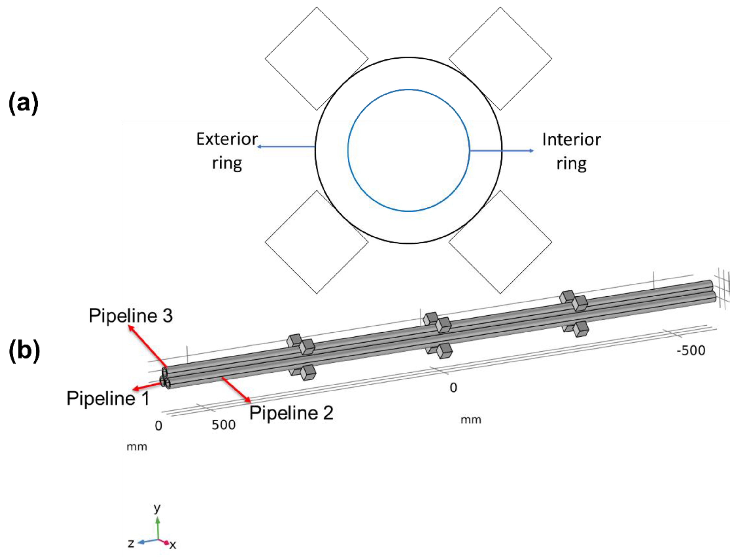
The magnetic field was produced by neodymium magnets (Nd₂Fe₁₄B of grade N33) of moderate intensity, corresponding to 5000 G (Socoter Ltd., Santiago, Chile), coated with Ni/Cu/Ni, having dimensions of 20 × 20 × 20 mm³. The strength of SMF was measured through an AC/DC Gaussmeter model PCE-MFM 3000 (PCE Americas Inc., Southampton, UK). The rare earth (RE) content in the RE–Fe alloy of the magnet, ranges between 30 to 35 Wt%. According to manufacture specifications, the corresponding remaining flux density B_r, coercivity values bH_c and jH_c, and maximum stored energy (BH)_max are, respectively 1.164 T, 11.43 kOe and 25.99 kOe, and 33.06 MGOe. The visual control of the SMF was performed by using COMSOL Multiphysics software v5.5. (Comsol Company, Stockholm, Sweden), which is described below.

2.4. Modeling the SMF

The considered geometry consists of three cylinders accounting for the pipelines and 3 sets of 4 cubes which are the magnets. Seawater flows through the pipelines with a mean speed of 1.35 ± 0.4 m/s determined in two steps. (1) Calculating the flow rate (Q) via measuring the time needed to fill a recipient. (2) Calculating the speed using $U=Q/A$, where $U$ is the magnitude of the velocity and $A$ is the section of the pipeline. In this case, $A$ = 2.5 cm². Then, $U$ = 1.38 m/s. Next step in the analysis is the calculation of the magnetic Reynolds number ($R{e}_m$). This number is defined through $R{e}_m=\left(UL\right)/\lambda$ [23], where $\lambda ={({\mu }_0{\sigma }_i)}^{-1}$ is the magnetic diffusivity, ${\mu }_0$ the magnetic permeability of vacuum and ${\sigma }_i$ is the fluid conductivity. The latter means that if $R{e}_m\ll 1$, the magnetic flux density $\mathit{B}$ influences the fluid velocity $\mathit{u}$; however, there is little influence of $\mathit{u}$ on $\mathit{B}$. It turns out that $R{e}_m\approx {10}^{-5}$, which is ≪ 1. Therefore, we computed the magnetic flux density $\mathit{B}$ in space using the magnetic fields no currents formulation, as the fluid will not affect $\mathit{B}$. In this case, $\mathit{B}$ is computed through the magnetic scalar potential ($\phi$). This formulation was used in the environment of COMSOL Multiphysics v5.5.

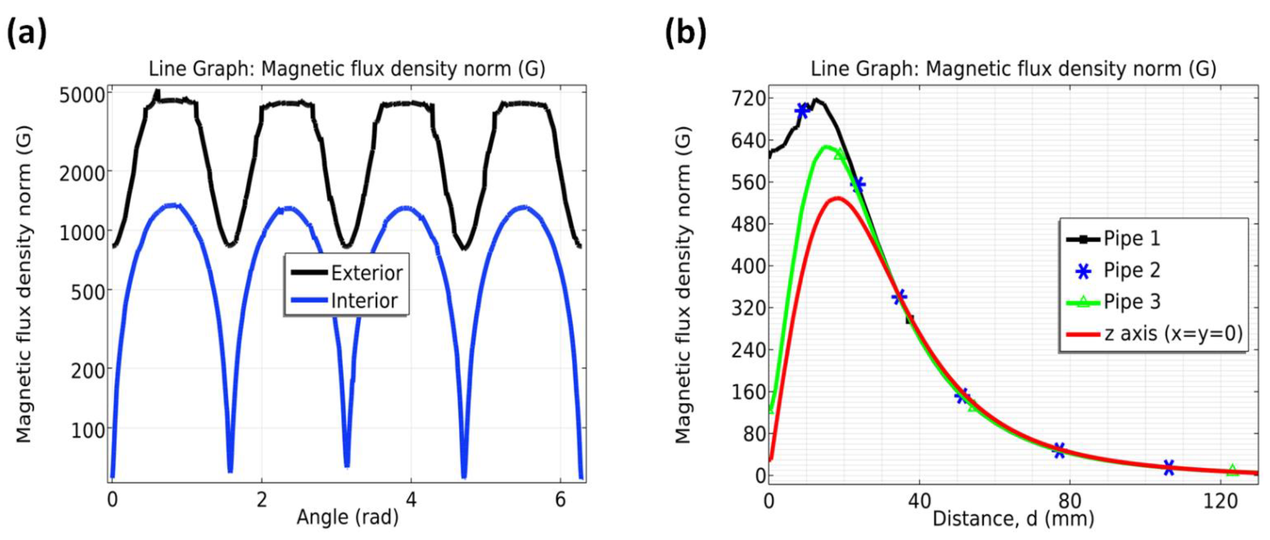
The measurements described in 2.3 were used with the aim to find the magnetization of the individual permanent magnets so that the magnetic fields no currents formulation can be defined. The components of $\mathit{B}$ at (x,y,z) away from the permanent magnet of dimensions 2a, 2b and 2c homogeneously magnetized along the z-direction, i.e. $\mathit{M}=M_0{\widehat{\mathit{e}}}_z$, can be found by evaluating the equations in [24,25]; see also [26] for a complete description. Accordingly, the analytical solution for $\mathit{B}$ in the magnetization axis can be expressed in terms of the magnetic permeability of the ferromagnetic material and geometrical dimensions of the magnet evaluated in a $t{g}^{-1}$ function. The orthogonal components to the magnetization show a logarithmic form. Simplifying equations, it can be reduced to Equation (1), for which $L=2a$, W = 2b, D = 2c are the length, width, and depth of a rectangular magnet, $B_r$ is the remanent flux density, $B_r=\mu M_0$, and d is the distance measured along the magnetization axis. A measurement at $x=L/2$, $y=W/2$ and$z>D$, allows finding $B_r$ or $M_0$.

$$\left|\mathit{B}\left(d\right)\right|=\frac{B_r}{\pi }\left\{arctan\left(\frac{L·W}{2d\sqrt{4d^2+L^2+W^2}}\right)-arctan\left(\frac{L·W}{2\left(D+d\right)\sqrt{4{(D+d)}^2+L^2+W^2}}\right)\right\}$$

(1)

Measuring $\left|\mathit{B}\right|$ at the side of each magnet via Gaussmeter, one finds B_r to then compute $\mathit{B}$ in space using COMSOL Multiphysics, based on the magnetic fields no currents formulation.

2.5. Measurement of Physicochemical Parameters

During the experimental SMF tests, daily measurements of physicochemical parameters of seawater in the effluent, including temperature (°C), pH, salinity (psu), electrical conductivity (S/m) and dissolved oxygen (mg/L), were performed by using a HI 98,194 multi-parameter probe (Hanna Instruments Inc., Woonsocket, RI, USA).

2.6. Biofilm Analysis

At the end of the 60 days of experimentation, the experimental pipes were removed to carry out the biofilm sampling. Once the pipes were removed, they were cut longitudinally, obtaining two parts. The biomass was obtained by scraping the surface. Subsequently, 100 mg of biomass was weighed and placed in test tubes with marine saline solution, followed by periods of sonication for 30 s, alternated by 30 s of ice bath. This process was repeated three times. After sonication, the supernatant of each sample was taken, and serial dilutions were made in marine saline solution.

2.6.1. Cell Viability

The quantification of viable bacteria was performed by means of epifluorescence microscopy using the 10⁻² working dilution with the LIVE/DEAD^® BacLightTM Bacterial Viability kit, according to the supplier’s instructions (cat. no. L7012, Thermofisher, Waltham, MA, USA), allowing the differentiation of live and dead bacteria present in the biomass to be removed from the experimental pipes.

2.6.2. Metagenomic Analysis

To evaluate the effect of SMF on the biofilm structure, and the microbial communities in the pipes with the treatments and the control condition were characterized after 60 days of operation in the A–W and S–S periods. The extraction of total DNA from biofilm collected from each test was performed by using the phenol:chloroform method [27]. The gDNA purification was subsequently performed, according to the UltraClean^® 15 DNA Purification Kit by MO BIO protocol (cat. no. 12100-300). The extraction was visualized on a 0.8% agarose gel stained with SYBR Safe DNA gel stain (INVITROGEN, Waltham, MA, USA) by using a 1 kb molecular weight marker (Fermentas, cat. no. SM0311). Total DNA samples were processed by the Laboratorio Genoma Mayor SpA. (Santiago, Chile) for metagenomic analysis by considering 16S rRNA and 18S rRNA marker genes on the Illumina MiSeq platform with 200,000 reads per sample and bioinformatic analysis. The analyzed data correspond to overlapping amplicon sequences obtained on the Illumina platform HiSeq 2 × 250 using the method described by Dr Knight’s lab [28]. These sequences correspond to 34 samples from the V3–V4 region of the 16S rDNA gene and 30 samples from the V4 region of 18S rDNA gene. The bioinformatic protocol of DADA2 on the R platform for sample analysis was used. The DADA2 package infers sequence variants of the accurate amplicon sequences (ASV) from amplicon sequencing data, replacing the OTU clustering approach. The DADA2 pipeline takes, as input, the fastq files demultiplexed and generates the sequence variants and their sample abundances after removing errors from substitution and chimera. The taxonomic classification is done through a native implementation of the naive Bayesian Classifier RDP, and the assignment of the 16S rDNA gene sequences is done by exact match.

2.7. Statistical Analysis

To evaluate the significance of variation of the species richness and their relative abundance by varying the SMF tests, the experimental data were processed using the univariate statistical analyses performed in Minitab 17 (Minitab LLC, State College, PA, USA). The analysis of biofilm composition was carried out by using a biological database composed of those OTUs that exhibited a frequency of occurrence over 20% during the period of study. A multivariate canonical redundancy analysis (RDA) was used to evaluate the influence of the environmental variables (temperature, salinity and DO) on the variance of species composition (and their relative abundance) during survey period (A–W, S–S), SMF tests (PPS, PCS) and C conditions. The significance of the ordination axes was evaluated by 500 Monte Carlo permutations [29]. This analysis was computed CANOCO version 4.5 (Biometrics-Plant Research International, Wageningen, The Netherlands).

3. Results

3.1. Characterization of the Pipeline Transportation System

A qualitative analysis of the SMF is reported in Figure 1. Both Figure 1b,c show the SMF characteristics in the surrounding area of the pipeline transportation system. The SMF vectors exhibit a marked variable direction very close to the magnetic source (Figure 1b). However, as the evaluation point for the SMF strength moves away from the source, the SMF becomes homogenous in areas distant from the magnets. The presence of three magnet rings in a row around the pipe generates repulsion forces that are responsible for causing the formation of the characteristic “rose petals” shape (Figure 1c), where the color scale indicates the SMF intensity that is maximum next to the magnets.

To obtain more insights about the SMF strength, Figure 2 shows the points where SMF was evaluated. Considering the X–Y plane (Figure 2a), two circumferences are drawn (black and blue color) and indicate the exterior and interior ring, respectively. The magnets are superimposed, since they correspond to each of the three magnet arrays, placed at different positions along the z-axis, as shown in Figure 1. Figure 2b displays the three pipelines, which are numbered, surrounded by an array of four magnets. An evaluation line is defined along the symmetry axis of each pipeline, and the symmetry line of the whole system along the z-axis is at x = y = 0.

Figure 3 reports the results of data elaboration performed with COMSOL software. Observing Figure 3, it can be noticed that the SMF intensity varies as a function of the angle (along the rings in Figure 2a): it is maximum next to the field source (magnet) and minimum at the midpoint between two magnets. At the point where the circumference with the largest radius (2.5 cm) is tangent to the magnets, a maximum SMF intensity close to 5000 G was found. This value agrees with the experimental measurements performed with the gaussmeter. When a radius smaller than 1 cm is detected, the SMF intensity decreases considerably, up to achieving a reduction by 70%, compared to the maximum value (Figure 3a). Therefore, the SMF profile along the HDPE pipe (according to the description in Figure 2b) presents points of maximum next to the magnet rings and a gradual decay in points that are more and more distant from the magnets. In points far from the magnets, the maximum SMF intensity ranges between 720 G and 520 G. At a distance longer than 120 mm from the magnet ring, the SMF intensity tends to be zero (Figure 3b).

The physicochemical parameters of the seawater flowing inside the pipeline transportation system were analyzed during the two survey periods, i.e., A–W and S–S (

Table 1. Physicochemical parameters of seawater measured during the tests.

Period	Test	T (°C)	pH	EC (µS/cm)	Salinity (p.s.u.)	D.O. (mg/L)
	C	16.2 ± 0.6	8.0 ± 0.1	52,741 ± 310	34.9 ± 0.2	6.3 ± 0.8
A–W	PPS	16.2 ± 0.6	8.0 ± 0.1	52,735 ± 310	34.8 ± 0.2	6.1 ± 0.7
	PCS	16.2 ± 0.6	8.0 ± 0.1	52,735 ± 315	34.8 ± 0.2	6.1 ± 0.8
	C	19.4 ± 0.7	7.7 ± 0.2	50,855 ± 420	33.6 ± 0.5	5.1 ± 0.5
S–S	PPS	19.0 ± 0.5	7.7 ± 0.2	50,203 ± 413	33.2 ± 0.4	5.4 ± 0.3
	PCS	19.0 ± 0.5	7.7 ± 0.2	50,203 ± 411	33.2 ± 0.4	5.4 ± 0.3

Notes: A–W, autumn–winter period of study; S–S, spring–summer period of study; T, temperature; EC, electrical conductivity; DO, dissolved oxygen.

). It was noticed that the temperature of the seawater flowing inside the pipelines remained constant around 16 °C from A–W and 19 °C from S–S. No significant differences in temperature profile were found comparing results from the three sets of tests, i.e., PPS, PCS and C during both survey periods (Table 1). From A–W, dissolved oxygen (DO) concentration was found equal to 6.3 mg/L in test C and 6.1 mg/L in the other two tests, whereas from S–S, the DO concentration was approximately 5.1 mg/L in test C, and 5.4 mg/L in the other two tests. Values of pH were detected equal and stable in all the tests conducted, showing a value of 8.0 from A–W and 7.7 from S–S. Salinity values were similar in both survey periods, i.e., 34.9 p.s.u. in test C during both survey periods and 34.8 p.s.u. in tests PPS and PCS from A–W and about 33 p.s.u. from S–S.

3.2. Cell Viability in Biofilms

The cell viability of bacteria forming the biofilm extracted from the inner surface of pipes of the experimental pipeline transportation system was evaluated by using the Live/Dead epifluorescence method. The number of live bacteria was significantly higher than those dead during both survey periods. In more details, during A–W, the highest number of live cells was detected for the test PPS (642,843 cells/cm²), compared to test PCS and test C (Figure 4a). It is also evident that only the PCS treatment showed a significantly lower number of live cells (419,318 cells/cm²), compared to the control (552,213 cells/cm²). Conversely, from S–S, the highest number of live cells was found for test PCS (Figure 4b) (757,780 cells/cm²), compared to test PPS (372,942 cells/cm²) and test C (421,489 cells/cm²), thus, showing a significant difference between them. On the other hand, no significant difference was noticed for the number of dead cells among all tests (Figure 4b).

3.3. Biofilm Composition

Metagenomic analysis revealed that during the survey periods (A–W and S–S), the bacterial biofilm community was composed of a total of 819 taxa, mainly represented by Proteobacteria, Bacteroidetes, Planctomycetes, Flavobacteriaceae and Fusobacteria groups. Among all taxa identified, 40 exhibited a frequency of occurrence higher than 20% during the A–W period, and 38 presented a frequency of occurrence and relative abundance higher than 20% and 2%, respectively, during S–S period. Therefore, all the statistical analyses were performed considering only these OTUs. During the A–W period, it was observed that most of the OTUs present in the control tests were tolerant to the two types of SMF disturbances applied (Figure 5a).

However, it can be observed that Bacillus spp. is only present in the control and is not representative in any of the treatments. In contrast, Arcticiflavibacter spp. and Marinicella spp. are present in the control and in both PPS and PCS treatments, but without significant differences in relative abundance (Figure 5a). In contrast, Sedimenticola spp., Lodidimonas spp., Sneathiella spp., Gracilimonas spp. and Lutimonas spp. are only present in PPS. In the PCS case it is also possible to find some species that are present only in this treatment, such as Colwellia spp. and Pseudofulvibacter spp. Only in the case of Arcobacter spp. was it possible to determine an increase in relative abundance in the PCS treatment, with respect to the control. In the opposite direction, it was possible to determine a decrease in relative abundance for Halioglobus spp. in the PCS treatment, with respect to the control (Figure 5a). For the S–S period it was possible to determine that only Candidatus tenderia was present in the control and in both treatments with a relative abundance without significant differences (Figure 5b). On the other hand, for Marinobacter spp. It was observed that despite being present in the control and in both treatments, a decrease in relative abundance was observed in the PPS treatment, with respect to the control condition. Other species, such as Kangiella spp. and Maribacter spp., are only present in the treatments and not in the control. It is also possible to highlight that in the PCS treatment, Pseudoalteromonas spp., Oceanospirillum spp., Marinicella, Lutimonas and Halodesulfovibrio spp. are maintained in the control and in the PCS treatment, without the presence of a relative abundance greater than 5% in the PPS treatment (Figure 5b). On the other hand, species, such as Marinobacter, Pseudoalteromonas, Lutimona and Marinicella, are present in both A–W and S–S periods studied. In addition, it was evidenced that Pseudoalteromonas is sensitive to the PPS treatment since in both study periods it was only observed in the control and in the PCS treatment (Figure 5).

A total number of 441 taxa of eukaryotes were identified in the biofilm community during the entire experimental period. The most representative groups were Protists, Nematodes, Arthropods and Ascidians. Among all taxa identified, only 17 of them showed a frequency of occurrence higher than 20% and a relative abundance higher than 2% during the A–W period, whereas during the S–S period, only 18 exhibited a frequency of occurrence over 20% and relative abundance higher than 2%. In general, the composition of the eukaryotes forming the biofilm during the A–W period (Figure 6a) did not vary significantly among all tests. Thus, Syndiniales, Stolidobranchia spp., Pleurosigma spp., Monhysterida spp., Harpacticoida spp. And Chromadorida spp. Are present in the control, as well as in both PPS and PCS treatments (Figure 6a). In contrast, Navicula spp. and Mammalia spp. were only present in the control and Lecudina spp. and Desmodorida spp. were only observed in the PCS treatment. Only in the case of Chromadorida was it possible to observe a significant increase in relative abundance in the PCS treatment with respect to the control, and for Pleurosigma there was a significant increase in the PPS treatment, with respect to the control (Figure 6a). For the S–S period, Enoplida spp., Cyclidium spp., Cryptocaryon spp. and Chlamydomyxa spp. were present in the control and in both treatments (Figure 6b). It is only possible to observe a significant decrease in relative abundance in PCS with respect to the control for Cyclidium. On the other hand, for Aplanochytrium spp. it was possible to determine a significant increase in relative abundance in the PPS only, with respect to the control (Figure 6b). It was also possible to determine that only Desmodorida is present in both A–W and S–S study periods.

With regard to bacterial species richness during the A–W period, no differences were observed among all tests (Figure 7a), whereas during the S–S period, a higher species richness was found in the PPS test than PCS and C tests (Figure 7a). Moreover, concerning the relative abundance of bacteria, once more no significant difference was observed among all tests during A–W period. On the contrary, during S–S period, the abundance observed in test C was higher than in tests PPS and PCS (Figure 7b).

About the eukaryote species richness, significant differences were observed among tests during the A–W and S–S periods (Figure 7c). More in detail, during the A–W period, a higher species richness was observed in test PPS than in tests PCS and C. Whereas during the S–S period, no differences in species richness were observed among all tests (Figure 7c). The relative abundance of eukaryotes (Figure 7d) showed a slight variation among all tests during the A–W period, whereas during S–S period, the relative abundance in test PPS was higher than in both PCS and C tests (Figure 7d).

Canonical redundancy analysis (RDA) showed that composition of the bacterial species community varied significantly during seasons. Significant increases of the relative abundance of several species were observed during the S–S period (Figure 8a) with species such as Candidatus_tenderia (Cnt), Marinifilum spp. (Mnf) and Spongibacterium spp. (Spo) present only during this survey period (Figure 8a). On the other hand, a higher species richness was detected during A–W, showing a significant increase in Articiflavibacter spp. (Afb) and Arcobacter spp. (Arb) abundance (Figure 8a). During the S–S period, the composition of bacteria from both tests PPS and PCS was similar. During the A–W period, Articiflavibacter spp. (Afb) was the most abundant species in test C, whereas in both tests PPS and PCS, this species was as abundant as others (Figure 8a). Moreover, a significant correlation between temperature and season was found, as well as an increase in dissolved oxygen (DO) that was evident during the A–W period (Figure 8a).

Canonical redundancy analysis (RDA) conducted for the eukaryote species showed that their composition varied significantly between seasons. Fragilidium spp. (Frg), Polykrikos spp. (Ply) and Parvilucifera spp. (Pvr) were only detected during the S–S period (Figure 8b), whereas Cercozoa spp. (Cer) and D2P04A09 spp. (D2p) were only found during the A–W period (Figure 8b).

4. Discussion

In this study, seawater temperature was influenced by seasonality despite the Humboldt Current influencing the San Jorge Bay in Antofagasta maintains relatively homogeneous the water temperatures throughout the year [8,30]. Therefore, during the A–W period, the temperature was 16.2 °C, while during the S–S period, the temperature was a little higher and equal to 19 °C, showing a relative difference up to 20%. 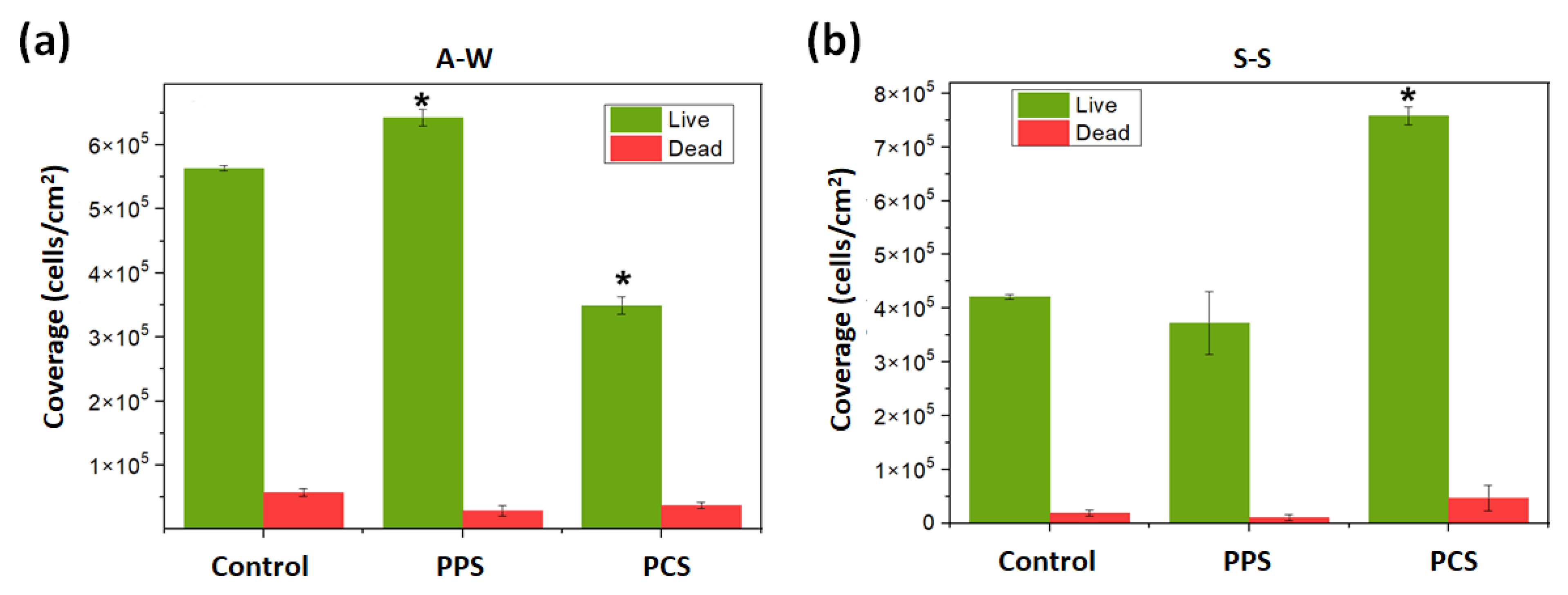The temperature influenced other parameters such as pH, electrical conductivity, salinity and DO, that showed higher values in the A–W period than in S–S (Table 1): differences between the two survey periods were less than 5% for pH, EC and salinity and approximately 20% for DO. During the same survey period, no significant difference among all environmental parameters was observed by varying the test (i.e., PCS, PPS and C), whereas the SMF significantly affected the cell viability of the biofilm extracted from the inner surface of pipes of the experimental pipeline transportation system (Figure 4). This result agrees with the three different effects that SMF can have on biofilm, as follows: (i) stimulatory; (ii) inhibitory, or (iii) unobservable [18] and with the different sensitiveness to SMF that each species can show. For example, Serrano et al. [31] determined that the enzymatic activity of superoxide dismutase (SOD) for the microalga Scenedesmus obliquus exhibited an increase in its activity as a response to a continuous-type SMF perturbation, whereas Nannochloropsis gaditana increased the enzymatic activity when exposed only to the pulse-type SMF perturbation. According to Sergio et al. [32], disturbances can alter interspecific interactions and produce community-level effects on species, thus, causing a decrease in biomass and cell viability, as well as changes in community structure and biodiversity.

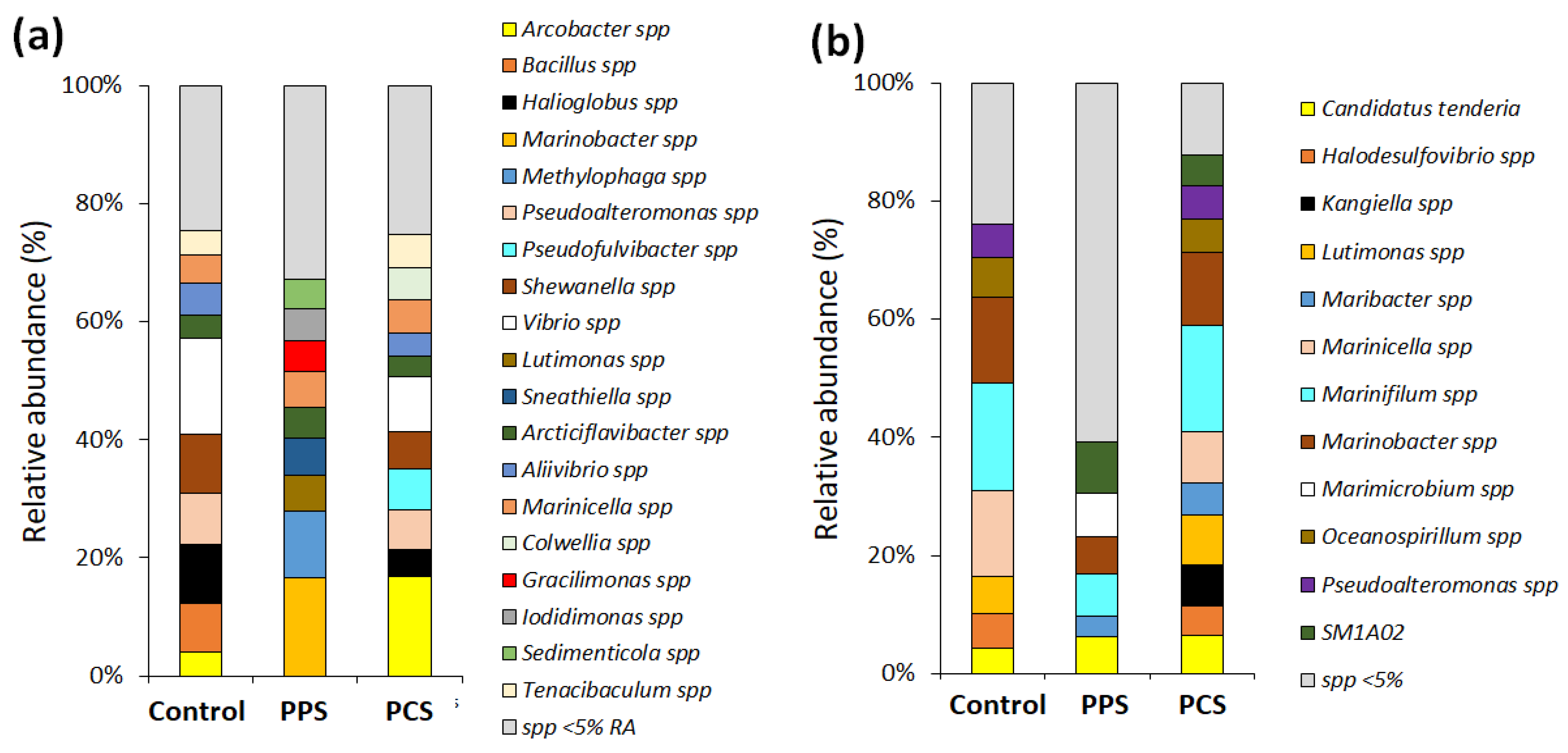
Through the metagenomic studies, the effects of SMFs on the biofilm composition were analyzed. The bacterial composition of the biofilm mainly consisted of OTUs belonging to families of γ-Proteobacteria, α-Proteobacteria, Bacteroidetes and Planctomycetes. These groups of bacteria are the main colonizers of marine biofilm, as highlighted in a study on materials of plastic origin, such as HDPE/LDPE immersed in seawater [33]. Carson et al. [34] demonstrated that microorganisms are particularly abundant on polystyrene material by electron microscopy, whereas Oberbeckmann et al. [35] basing their conclusions on DGGE band variation, suggested that polymer composition not only influences the abundance of attached microorganisms, but also affects the community structure of the biofilm. Results from the present work have highlighted that the variability of OTUs in the control tests depends on seasonality, whereas SMF disturbances did not significantly affect the community behavior. The variability of OTUs in results from tests PPS and PCS during each survey period depends on the sensitivity and tolerance of each species to the magnetic intensity gradient as well as type of perturbation (pulse or continuous). Arcticiflavibacter spp. and SM1A02 spp. were found only in SMF tests, whereas they were absent in test C. Genera sensitive to SMF disturbance, and they are negatively affected and, therefore, replaced by more tolerant genera, such as the Arcobacter spp. that is abundant in both PPS and PCS tests (Figure 4a).

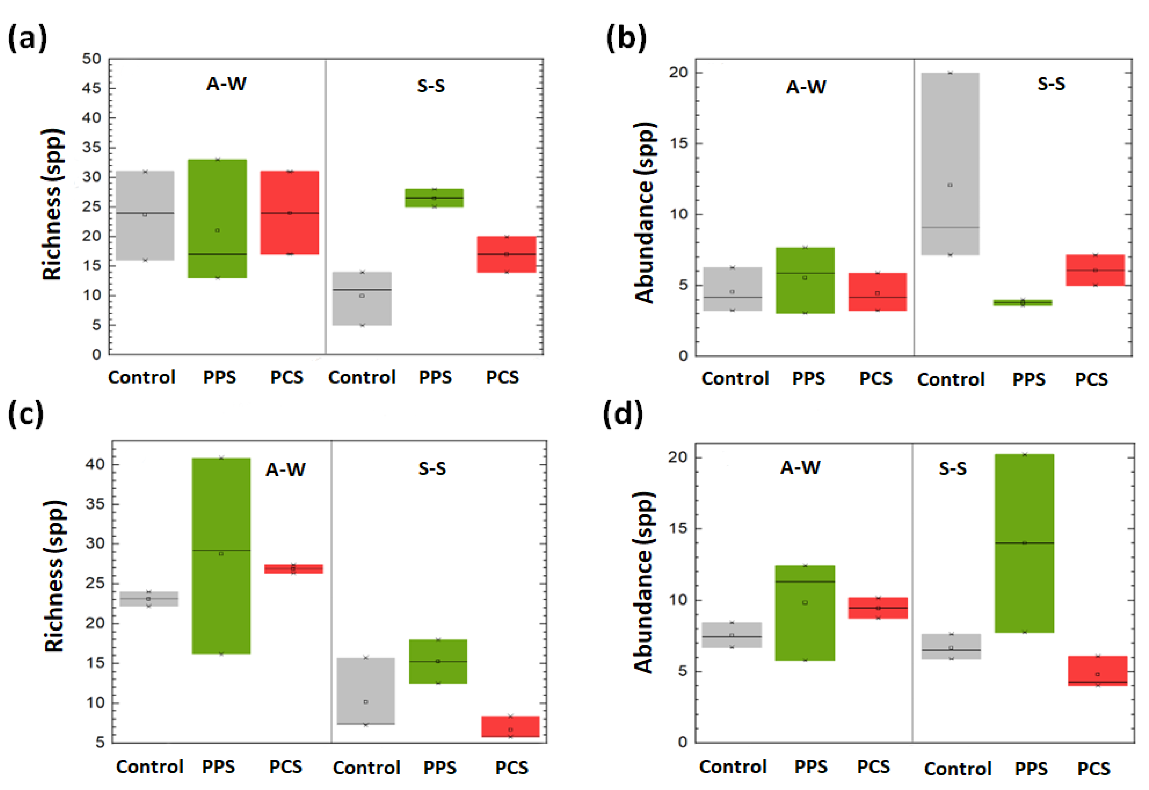
Regarding to the richness and relative abundance of OTUs, no relevant effects among all tests were observed during the A–W period. However, during the S–S period, a higher richness of OTUs was found in test PPS than PCS and C tests. This result is a consequence of the effects of SMF on the species that take part to the biofilm colonization and attachment process, thus, governing the mechanisms responsible for the diversifications in community composition by varying the SMF perturbation. On the contrary, the relative abundance of species during the S–S period was higher in test C than test PPS. Therefore, test PPS was characterized for exhibiting a great richness of species, as well as a low relative abundance. This controversial result is caused by the stress that SMF induces on microbial community that constantly must adapt to and recover from the changes of the environmental conditions.

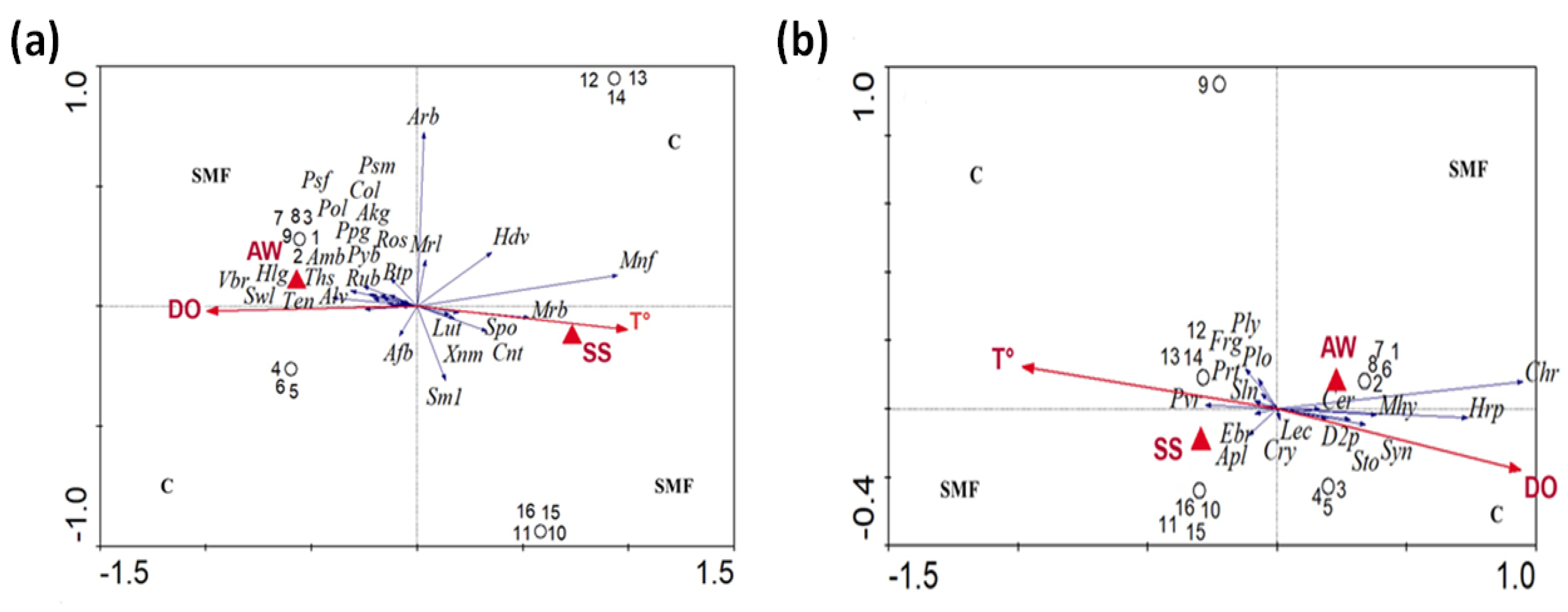
Canonical redundancy analysis (RDA) showed a significant difference in bacterial composition between SMF tests and C test. The relative abundance of OTUs observed during the S–S period was significantly different between the two group of tests, i.e., under SMF perturbation and control. In both cases, OTUs are positively correlated with temperatures that represents a key factor for biofilm growth, as well as abundance on sediments surface layers, as found by Battin et al. [36]. Conversely, a significant positive correlation between DO concentration and richness of OTUs was observed during the A–W period. This result is in agreement with those from Kress and Herut [37]. In test C, the relative abundance of an unique OTU was found, whereas in SMF tests, relative abundances of 17 OTUs were detected, thus, showing that the species richness of these tests is positively correlated with seasonality and DO concentration. Similar results were obtained by Kohno et al. [38] in studying the effects of SMF perturbations on Staphylococcus aureus and Escherichia coli mutants under aerobic and anaerobic conditions, thus, proving that bacterial growth was only inhibited by SMF under anaerobic conditions, whereas no effect was observed under aerobic conditions.

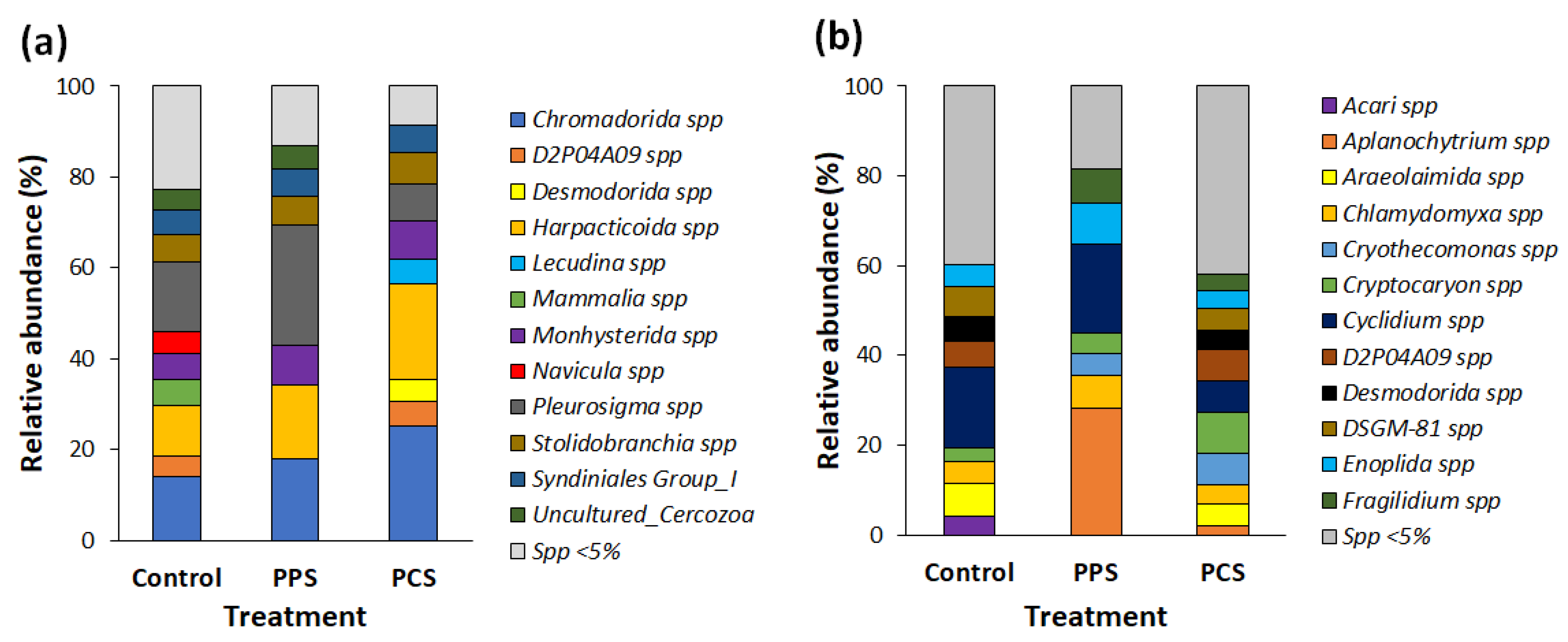
As concerns the composition of eukaryotes, mainly protists and invertebrate larvae were detected, whereas no relevant differences were observed in the composition of OTUs in biofilm between SMF tests and C test. Moreover, the richness of OTUs in test PPS was higher during the A–W period than during the S–S period. Relative abundance was the highest in the PPS test during both survey periods. Finally, RDA showed evident differences in bacteria composition between seasons as well as among the tests, i.e., PPS, PCS and C (Figure 7b).

As was noticed for bacterial community, the relative abundance of eukaryotic OTUs during the S–S period was correlated with temperature, whereas during the A–W period, it was correlated with DO. Conversely to results from studies on bacteria, the highest richness of eukaryote OTUs was found in test C during the S–S period. According to this result, studies from the literature have showed that among all marine protists, ecologically redundant taxa or dormant species have the potential to increase considerably in number after an environmental perturbation more than other species [39]. Conversely, many rare taxa may contribute stronger to microbial community dynamics despite their low proportional abundance [40,41]. In this study, Aplanochytrium spp. (belonging to the Stramenopiles), a protist not very abundant in seawater, increased its relative abundance under SMF conditions during the S–S period. It has been described as participating in prey–predator interactions in the grazing food web of the marine ecosystem [42]. Additionally, evidence have showed that some specialized OTUs belonging mainly to parasites (Cercozoa and MALV) thrive in specific seasonal periods, thus, abruptly increasing their abundance [39]. In general, Cercozoa both as generalists and as specialists, compose an important group of the protist community, thus, generating connections with a variety of other protists and influencing trophic pathways through parasitism [41]. Although the dynamics of eukaryotes exhibited in SMF tests, as well as in test C, prove that the diversification of OTUs are related to their tolerance and adaptation skills to SMF, Hadfield et al. [43] indicate that the colonization of eukaryotic microorganisms or invertebrate larvae also strongly depends on the composition of the primary biofilm.

5. Conclusions

This paper shows the results of the effect of SMF on the marine microbial communities colonizing pipelines for seawater transportation. Depending on the type of perturbation, i.e., pulse-type or continuous-type, and seasonality, the communities forming the biofilm show different dynamics. The cell viability of bacteria in biofilms colonizing the inner surface of the transport pipes was evaluated in the S–S and A–W periods, showing that the number of live bacteria was higher than the number of dead bacteria. During the S–S period, the highest number of live cells (757,780 cells/cm²) was detected under PCS, while in the A–W period it was detected under PPS (642,843 cells/cm²), and the lowest viability (349,151 cells/cm²) was obtained under PCS. This would indicate that during the A–W period, pulse-type perturbation stimulated the microorganisms’ growth, whereas continuous-type perturbation reduced the growth rate. During the S–S period, continuous-type perturbation stimulated the growth of microorganisms while pulse-type perturbation did not generate effects. Moreover, the microorganisms’ community composition was affected by the skill of species to adapt to external perturbations produced by SMF, as well as by seasonal and environmental factors. Metagenomic analysis showed the presence of 819 taxa for bacteria and 441 taxa for eukaryotes in both A–W and S–S sampling periods. In the case of bacteria, only 40 taxa in the A–W period and 38 taxa in the S–S period exhibited a frequency of occurrence greater than 20%, but only 12 OTUs presented relative abundances higher to 5% in S–S (see Figure 5b). In the case of eukaryotes, the most representative groups were Protists, Nematodes, Arthropods and Ascidians. Among them, only 17 taxa in the A–W period and 18 taxa in the S–S period presented a relative abundance greater than 2%. RDA showed that composition of the bacterial community varied significantly during the annual seasonality, with a significant increase in the relative abundance of OTUs, such as Candidatus tenderia or Marinifilum during the S–S period, while in the A–W period, Articiflavibacter spp. and Arcobacter spp. were the most abundant. As regards eukaryote, the RDA resulted in the same trend showed by microorganisms’ composition: eukaryotes’ composition varied significantly with annual seasonality, for example, Acari spp., Fragilidium spp. and Aplanochytrium spp. were only detected during the S–S period, while Cercozoa were found only during the A–W period.

This research work demonstrates that SMF is capable of directly affecting the composition of biofilms attached to the inner surface of pipelines, transporting seawater and indirectly of the phenomena of biofouling that is due to extracellular polymeric substances (EPS), as the amount and chemical composition of EPS secreted by microorganisms depend on several factors, including microorganism’s strains and abundance. Moreover, results from this study have highlighted that SMF effects on biofilm formation and composition also depend on operating conditions, such as the biodiversity of the geographical region, the position of magnets, the intensity of the SMF, the time of service and the seasonality. Therefore, further studies that are focused on aspects relating to the amount and composition of EPS, as well as the operating conditions of SMF application, are necessary to deeply understand the real potentiality of this treatment to prevent the biofouling formation.

References

1. Jones, E.; Qadir, M.; van Vliet, M.T.; Smakhtin, V.; Kang, S.-M. The state of desalination and brine production: A global outlook. Sci. Total Environ. 2018, 657, 1343–1356. [Google Scholar] [CrossRef] [PubMed]
2. Herrera-León, S.; Lucay, F.; Kraslawski, A.; Cisternas, L.A.; Gálvez, E.D. Optimization approach to designing water supply systems in non-coastal areas suffering from water scarcity. Water Resour. Manag. 2018, 32, 2457–2473. [Google Scholar] [CrossRef]
3. Herrera-León, S.; Cruz, C.; Kraslawski, A.; Cisternas, L.A. Current situation and major challenges of desalination in Chile. Desalination Water Treat. 2019, 171, 93–104. [Google Scholar] [CrossRef]
4. Al-Juboori, R.A.; Yusaf, T. Biofouling in RO system: Mechanisms, monitoring and controlling. Desalination 2012, 302, 1–23. [Google Scholar] [CrossRef]
5. Momba, M.N.B.; Kfir, R.; Venter, S.N.; Cloete, T.E. An overview of biofilm formation in distribution systems and its impact on the deterioration of water quality. Water SA 2000, 26, 59–66. [Google Scholar]
6. Vergara, O.A.; Echevín, V.; Sepúlveda, H.H.; Quiñones, R.A. Controlling factors of the seasonal variability of productivity in the southern Humboldt Current System (30–40° S): A biophysical modeling approach. Cont. Shelf Res. 2017, 148, 89–103. [Google Scholar] [CrossRef]
7. De Carvalho, C.C.C.R. Marine biofilms: A successful microbial strategy with economic implications. Front. Mar. Sci. 2018, 5, 126. [Google Scholar] [CrossRef] [Green Version]
8. Salta, M.; Wharton, J.; Blache, Y.; Stokes, K.R.; Briand, J.-F. Marine biofilms on artificial surfaces: Structure and dynamics. Environ. Microbiol. 2013, 15, 2879–2893. [Google Scholar] [CrossRef] [PubMed]
9. Zhang, W.; Ding, W.; Li, Y.-X.; Tam, C.; Bougouffa, S.; Wang, R.; Pei, B.; Chiang, H.; Leung, P.; Lu, Y.; et al. Marine biofilms constitute a bank of hidden microbial diversity and functional potential. Nat. Commun. 2019, 10, 517. [Google Scholar] [CrossRef] [Green Version]
10. Wang, S.; Su, X.; Cui, H.; Wang, M.; Hu, X.; Ding, W.; Zhang, W. Microbial richness of marine biofilms revealed by sequencing full-length 16S rRNA genes. Genes 2022, 13, 1050. [Google Scholar] [CrossRef] [PubMed]
11. Singer, A.; Johst, K. Transience after disturbance: Obligate species recovery dynamics depend on disturbance duration. Theor. Popul. Biol. 2017, 115, 81–88. [Google Scholar] [CrossRef] [PubMed]
12. Paine, R.T.; Tegner, M.J.; Johnson, E. Ecological surprises. Ecosystems 1998, 1, 535–545. [Google Scholar] [CrossRef]
13. Watanabe, K.; Yoshimura, C.; Omura, T. Stochastic model for recovery prediction of macroinvertebrates following a pulse-disturbance in river. Ecol. Model. 2005, 189, 396–412. [Google Scholar] [CrossRef]
14. Gould, J.L. Magnetoreception. Curr. Biol. 2010, 20, R431–R435. [Google Scholar] [CrossRef] [PubMed] [Green Version]
15. Fedele, G.; Green, E.W.; Rosato, E.; Kyriacou, C.P. An electromagnetic field disrupts negative geotaxis in Drosophila via a CRY-dependent pathway. Nat. Commun. 2014, 5, 4391. [Google Scholar] [CrossRef] [Green Version]
16. Ji, W.; Huang, H.; Deng, A.; Pan, C. Effects of static magnetic fields on Escherichia coli. Micron 2009, 40, 894–898. [Google Scholar] [CrossRef]
17. Albertini, M.C.; Accorsi, A.; Citterio, B.; Burattini, S.; Piacentini, M.P.; Uguccioni, F.; Piatti, E. Morphological and biochemical modifications induced by a static magnetic field on Fusarium culmorum. Biochimie 2003, 85, 963–970. [Google Scholar] [CrossRef]
18. Anaya, M.; Barbará, E.; Padrón, J.; Borrego, S.F.; Valdés, O.; Molina, A. Influencia del campo magnético sobre el crecimiento de microorganismos patógenos aislados ambiente del Archivo Nacional de la República de Cuba. Biomedica 2015, 35, 325–336. [Google Scholar] [CrossRef] [Green Version]
19. Insua, A. Magnetically treated water effect on biological processes. Rev. Elecetronica Vet. 2009, 10, 040916. [Google Scholar]
20. Raouia, H.; Hamida, B.; Khadidja, A.; Ahmed, L.; Abdelwaheb, C. Effect of static magnetic field (200 mT) on biofilm formation in Pseudomonas aeruginosa. Arch. Microbiol. 2019, 202, 77–83. [Google Scholar] [CrossRef]
21. Li, C.; Wang, L.; Liu, H. Enhanced redox conductivity and enriched Geobacteraceae of exoelectrogenic biofilms in response to static magnetic field. Appl. Microbiol. Biotechnol. 2018, 102, 7611–7621. [Google Scholar] [CrossRef] [PubMed]
22. Letuta, U.G.; Tikhonova, T.A. Magnetic fields and magnetic isotope 25Mg effects on biofilms formation by bacteria E. coli. Dokl. Biochem. Biophys. 2019, 484, 85–87. [Google Scholar] [CrossRef] [PubMed]
23. Davidson, P.A. Kinematics of MHD: Advection and diffusion of a magnetic field. In An Introd. To Magnetohydrodyn; Cambridge University Press: Cambridge, UK, 2010; pp. 102–106. [Google Scholar] [CrossRef]
24. Yang, Z.J.; Johansen, T.H.; Bratsberg, H.; Helgesen, G.; Skjeltorp, A.T. Potential and force between a magnet and a bulk Y1Ba2Cu3O7-δsuperconductor studied by a mechanical pendulum. Supercond. Sci. Technol. 1990, 3, 591–597. [Google Scholar] [CrossRef]
25. Camacho, J.M.; Sosa, V. Alternative method to calculate the magnetic field of permanent magnets with azimuthal symmetry. Rev. Mex. Fis. E. 2013, 59, 8–17. [Google Scholar]
26. Furlani, E.P. Permanent Magnet and Electromechanical Devices: Materials, Analysis, and Applications; Academic Press: Cambridge, MA, USA, 2001. [Google Scholar]
27. Sambrook, J.; Fritsch, E.R.; Maniatis, T. Molecular Cloning A Laboratory Manual (2nd ed.). Cold Spring Harbor, NY Cold Spring Harbor Laboratory Press, 1989-References-Scientific Research Publishing. Available online: https://www.scirp.org/(S(i43dyn45teexjx455qlt3d2q))/reference/ReferencesPapers.aspx?ReferenceID=1480044 (accessed on 28 April 2022).
28. Caporaso, J.G.; Lauber, C.L.; Walters, W.A.; Berg-Lyons, D.; Lozupone, C.A.; Turnbaugh, P.J.; Fierer, N.; Knight, R. Global patterns of 16S rRNA diversity at a depth of millions of sequences per sample. Proc. Natl. Acad. Sci. USA 2011, 108 (Supp. S1), 4516–4522. [Google Scholar] [CrossRef] [Green Version]
29. Ter Braak, C.J.F.; Smilauer, P. CANOCO Reference Manual and CanoDraw for Windows User’s Guide: Software for Canonical Community Ordination (version 4.5); Wageningen University&Research: Ithaca, NY, USA, 2002. [Google Scholar]
30. Gutiérrez, D.; Akester, M.; Naranjo, L. Productivity and sustainable management of the Humboldt current large marine ecosystem under climate change. Environ. Dev. 2016, 17, 126–144. [Google Scholar] [CrossRef]
31. Serrano, G.; Miranda-Ostojic, C.; Ferrada, P.; Wulff-Zotelle, C.; Maureira, A.; Fuentealba, E.; Gallardo, K.; Zapata, M.; Rivas, M. Response to static magnetic field-induced stress in Scenedesmus obliquus and Nannochloropsis gaditana. Mar. Drugs 2021, 19, 527. [Google Scholar] [CrossRef]
32. Sergio, F.; Blas, J.; Hiraldo, F. Animal responses to natural disturbance and climate extremes: A review. Glob. Planet. Chang. 2018, 161, 28–40. [Google Scholar] [CrossRef]
33. Sudhakar, M.; Doble, M.; Murthy, P.S.; Venkatesan, R. Marine microbe-mediated biodegradation of low- and high-density polyethylenes. Int. Biodeterior. Biodegradation 2008, 61, 203–213. [Google Scholar] [CrossRef]
34. Carson, H.S.; Nerheim, M.S.; Carroll, K.A.; Eriksen, M. The plastic-associated microorganisms of the North Pacific Gyre. Mar. Pollut. Bull. 2013, 75, 126–132. [Google Scholar] [CrossRef]
35. Oberbeckmann, S.; Loeder, M.G.; Gerdts, G.; Osborn, A.M. Spatial and seasonal variation in diversity and structure of microbial biofilms on marine plastics in Northern European waters. FEMS Microbiol. Ecol. 2014, 90, 478–492. [Google Scholar] [CrossRef]
36. Battin, T.J.; Wille, A.; Sattler, B.; Psenner, R. Phylogenetic and functional heterogeneity of sediment biofilms along environmental gradients in a glacial stream. Appl. Environ. Microbiol. 2001, 67, 799–807. [Google Scholar] [CrossRef]
37. Kress, N.; Herut, B. Spatial and seasonal evolution of dissolved oxygen and nutrients in the Southern Levantine Basin (Eastern Mediterranean Sea): Chemical characterization of the water masses and inferences on the N:P ratios. Deep Sea Res. Part I Oceanogr. Res. Pap. 2001, 48, 2347–2372. [Google Scholar] [CrossRef]
38. Kohno, M.; Yamazaki, M.; Kimura, I.; Wada, M. Effect of static magnetic fields on bacteria: Streptococcus mutans, Staphylococcus aureus, and Escherichia coli. Pathophysiology 2000, 7, 143–148. [Google Scholar] [CrossRef]
39. Caron, D.; Countway, P. Hypotheses on the role of the protistan rare biosphere in a changing world. Aquat. Microb. Ecol. 2009, 57, 227–238. [Google Scholar] [CrossRef] [Green Version]
40. Shade, A.; Jones, S.E.; Caporaso, J.G.; Handelsman, J.; Knight, R.; Fierer, N.; Gilbert, J.A. Conditionally rare taxa disproportionately contribute to temporal changes in microbial diversity. MBio 2014, 5, e01371-14. [Google Scholar] [CrossRef] [Green Version]
41. Genitsaris, S.; Monchy, S.; Viscogliosi, E.; Sime-Ngando, T.; Ferreira, S.; Christaki, U. Seasonal variations of marine protist community structure based on taxon-specific traits using the eastern English Channel as a model coastal system. FEMS Microbiol. Ecol. 2015, 91, fiv034. [Google Scholar] [CrossRef]
42. Hamamoto, Y.; Honda, D. Nutritional intake of Aplanochytrium (Labyrinthulea, Stramenopiles) from living diatoms revealed by culture experiments suggesting the new prey–predator interactions in the grazing food web of the marine ecosystem. PLoS ONE 2019, 14, e0208941. [Google Scholar] [CrossRef]
43. Hadfield, M.G. Biofilms and marine invertebrate larvae: What bacteria produce that larvae use to choose settlement sites. Annu. Rev. Mar. Sci. 2011, 3, 453–470. [Google Scholar] [CrossRef]
Figure 1. Characterization of the static magnetic field (SMF) in experimental pipeline transportation system. (a) picture of the pipeline transportation system used to perform SMF tests; (b) direction of the SMF (red arrows); (c) shape of the SMF (blue lines).
Water 14 03362 g001
Figure 2. (a) Cross section view in the X–Y plane showing two rings where the SMF is evaluated. (b) Sketch of the three pipelines surrounded by the magnets. An evaluation line is defined as the symmetry axis of each pipeline and another evaluation line, which is the symmetry axis of the whole system, along the z-coordinate.
Water 14 03362 g002
Figure 3. (a) Magnetic field strength around an outer circumference of a radius such that it is tangent to each of the inner sides of the magnets (black) and SMF strength around a circumference of an in-ner radius that is 65% of the outer radius and intersects the pipes (blue). (b) SMF strength gradient along the symmetry axis of the experimental pipes and SMF strength along the symmetry axis of the three pipes.
Water 14 03362 g003
Figure 4. Viability coverage of bacteria with Live/Dead staining during experimental studies. (a) A–W period and (b) S–S period. Experimental pipelines exposed to pulse-type SMF (PPS), continuous-type (PCS) and control (C) condition. (*) is referred to the significant difference by 95% confidence. The error bars correspond to the standard deviation of the triplicate of each of the samples analyzed.
Water 14 03362 g004
Figure 5. Relative abundances of top genera of bacteria forming biofilm showing relative abundance >5% in the pulse type SMF tests (PPS), continuous type SMF tests (PCS) and control (C) conditions in survey periods. (a) Autumn–Winter period; (b) Spring–Summer period.
Water 14 03362 g005
Figure 6. Relative abundances of top genera of eukaryotes forming the biofilm of the SMF pulse type (PPS), continuous type (PCS) and (C) control tests during the survey periods with relative abundance >5%. (a) Autumn–Winter period and (b) Spring–Summer period.
Water 14 03362 g006
Figure 7. Richness and relative abundance of species identified with the 16S rRNA gene (a,b) and with the 18S rRNA gene (c,d) in both survey periods of exposure to pulse-type (PPS) and continuous-type (PCS) SMF perturbations. The control group was not exposed to SMF.
Water 14 03362 g007
Figure 8. Canonical Redundancy Analysis (RDA) conducted for bacteria (a) and eukaryotes (b), according to the environmental conditions (i.e., temperature and dissolved oxygen concentration), and OTU abundance during Autumn–Winter (A–W) and Spring–Summer (S–S) survey periods under both static magnetic field (SMF) perturbations and control (C). OTUs bacteria (a): Aliivibrio (Alv), Aliikangiella (Akg), Amylibacter (Amb), Arcobacter (Arb), Arcticiflavibacter (Afb), Blastopirellula (Btp), Candidatus_tenderia (Cnt), Colwellia (col), Halioglobus (Hlg), Halodesulfovibrio (Hdv), Lutimonas (Lut), Marinicella (Mrl), Marinifilum (Mnf), Marinobacter (Mrb), Polaribacter_4 (Pol), Propionigenium (Ppg), Pseudoalteromonas (Psm), Pseudofulvibacter (Psf), Psychrilyobacter (Pyb), Roseibacillus (Ros), Rubripirellula (Rub), Shewanella (Swl), SM1A02 (Sm1), Spongiibacterium (Spo), Tenacibaculum (Ten), Thalassotalea (Ths), Vibrio (Vbr), Xanthomarina (Xnm). OTUS eukaryotes (b): Aplanochytrium (Apl), Cercozoa (Cer), Chromadorida (Chr), Cryothecomonas (Cry), D2P04A09 (D2p), Ebria (Ebr), Fragilidium (Frg), Harpacticoida (Hrp), Lecudina (Lec), Monhysterida (Mhy), Parvilucifera (Pvr), Ploimida (Plo), Polykrikos (Ply), Protoperidinium (Prt), Selenidium (Sln), Stolidobranchia (Sto), Syndiniales (Syn). DO, dissolved oxygen; T, temperature.
Water 14 03362 g008