
A Multi-Model Multi-Scale Approach to Estimate the Impact of the 2007 Large-Scale Forest Fires in Peloponnese, Greece

1
School of Rural, Surveying and Geoinformatics Engineering, National Technical University of Athens, 15780 Athens, Greece
2
Department of Civil Engineering, University of Bristol, Bristol BS8 1TR, UK
*
Author to whom correspondence should be addressed.
Water 2022, 14(20), 3348; https://doi.org/10.3390/w14203348
Submission received: 18 June 2022
/
Revised: 5 September 2022
/
Accepted: 13 October 2022
/
Published: 21 October 2022
(This article belongs to the Section Hydrology)
Abstract
:The hydrological impact of large-scale forest fires in a large basin is investigated on both a daily and an hourly basis. A basin of 877 km2 was chosen, with 37% of its area having been burnt in the summer of 2007. Five models are employed, namely SWAT (semi-distributed), GR4J, GR5J, and GR6J (lumped) for the daily time step, and HEC-HMS (semi-distributed) for the hourly time step. As SWAT and HEC-HMS implement the SCS-CN method, the change in the Curve Number (CN) from pre-fire to post-fire conditions is estimated along with the post-fire trend of CN for both time steps. Regarding the daily time step, a 20% post-fire increase in CN proved necessary for the accurate streamflow prediction, whereas ignoring this led to an underestimation of 22% on average. On an hourly time basis, CN was 95 for burnt areas after the fire, with a mildly decreasing trend after the third year and still above 90 until the fifth year. When neglecting this, peak flow is seriously underestimated (35–70%). The post-fire trend lines of CN for the two-time steps showed statistically equal slopes. Finally, GR models accurately predicted runoff while constraining one model parameter, which proved useful for the realistic prediction of other variables.
1. Introduction
The effects on hydrological processes of forest fires have been studied by many researchers for more than fifty years since the appearance of work by Rycroft [1] and Colman [2]. It is known that of all the components of the water cycle, runoff, infiltration, evapotranspiration, and erosion are those that are most influenced by forest fires. The vast majority of relevant studies examine the fire effects on small basins (smaller than 50 km2) [3,4,5,6,7,8], as systematic measurements from large basins are rarely acquired for both the pre-fire and post-fire periods [9,10,11]. The common method to deal with the assessment of the impact of forest fires is the well-known paired catchment method for response to fires [4,11,12,13,14,15,16,17]. In that method, two similar basins are used, one burnt and the other unburnt, in order to compare the results before and after a forest fire, either a wildfire or a prescribed one. However, test basins are usually of a small size [13,18,19]. In some studies, owing to the lack of data for the pre-fire period, gauges were established after the fires in both burnt and unburnt areas, which enabled comparisons of the basin response [18]. Of course, this is a variant of the paired catchment approach. Some other researchers chose to relate rainfall intensity to peak discharge data from detailed measurements in a multi-year post-fire period (e.g., [9]). Again, burnt areas are generally small.
An alternative approach to studying the effects of large-scale forest fires is to use hydrological models in order to simulate post-fire basin responses to real or hypothetical fires [3,20,21,22]. This becomes the only alternative when dealing with the impact of other factors acting simultaneously with fires, e.g., climate change [23].
Regarding the timescale, knowledge about the impact of fires on daily streamflow is quite limited [3,8,21], while fire effects on peak flows have not yet been studied extensively in large basins. Thus, the main objective of this study is to enhance the existing knowledge regarding the impact of fires on streamflow in large basins, both on a daily and sub-daily timescale and their possible interconnection. By adopting the approach of the use of hydrological models, the aforementioned impact of fires is translated into model parameter changes that are required for the reproduction of observed post-fire flows. This inevitably relates results to a specific model. In this work, we try to avoid using only one specific model, as will be explained next.
The most common method used within the frame of the adopted approach is the SCS Curve Number method [6,24,25,26,27,28,29], as this is quite simple and can simulate the effect of land use change (see description in Section 2.2). However, there is no universally accepted approach for the selection of a Curve Number (CN) for burnt areas. In the above-mentioned studies, the researchers estimated the values of CN for post-fire conditions. In particular, Cydzik and Hogue [26] estimated the post-fire CN for a small basin (51 km2) in California using HEC-HMS. Papathanasiou et al. [28] estimated the post-fire CN for three fire scenarios and a real fire event in a basin with an area of 127 km2, whereas McLin [30] estimated CN using HEC-HMS for a burnt area of 174 km2 in Los Alamos. Havel et al. [31] used SWAT to estimate the changes in total annual volume for runoff and other hydrological variables and, then, they correlated the magnitude of changes with the percentage of burnt area. To this end, those authors used multiple sub-catchments with areas ranging from 5 km2 to 270 km2. However, their study was based on data for only one year after the fire. Finally, NRCS [32] provides guidance for selecting the values of CN for various classes of soil burn severity.
Given the above, our first choice is the SCS-CN method, which by far constitutes the most widely used method for estimating streamflow volume; besides, linking the fire effect to only one parameter, such as CN, can hopefully minimize model equifinality [33,34]. Despite the studies in which Curve Number is estimated for post-fire flood events, insufficient knowledge exists regarding the values of CN for burnt areas on the daily time step. Additionally, it is expected that CN is dependent on a timescale through an unknown relationship. In this work, we employ two models that incorporate the SCS-CN method, namely SWAT [35,36,37] for the daily time step and HEC-HMS for the hourly time step. The assets of these two models are that they have been extensively used to simulate land use changes and the hydrological impact of fires, e.g., [6,24,25,26,28,38,39,40,41,42,43,44].
Although the SCS-CN method has been extensively employed as mentioned above, we believe that using a single model may provide a partial view of the fire effect on rates of total flow and other hydrological variables, such as percolation and evapotranspiration. To remedy this, we adopt the multi-model approach that has emerged in the last two decades. For example, Goswami et al. [45] in their work on regionalisation for flow prediction in ungauged basins provide an excellent summary of the arguments for using a multi-model approach, which are valid also for our work. Specifically, in that paper it is stated that “it is recognised that (i) the plurality of models and modelling approaches may be valid for the same catchment and application [46], (ii) each model has its inherent strengths and weaknesses, (iii) each makes use of different information, processing different forms of knowledge, and (iv) it is possible to use a number of models simultaneously whereby the strengths of individual models are pooled and perceptible weaknesses de-emphasised to produce a consensus output.”
In this vein, in addition to SWAT and HEC-HMS, we also use three lumped models from the Suite of GR hydrological models for precipitation-runoff modelling. These models are selected with the purpose for covering a wide spectrum of model structures, given that GR models are radically different from those that are based on the SCS-CN method.
All selected models are of the conceptual type. While models incorporating knowledge on the physics of fire effects on catchments, e.g., the Macaque models [44,47] are intuitively more attractive. In this work we preferred models of wide use that have been implemented within well-tested computer packages. Regarding to data requirements, although a number of recent studies make use of remote sensing products [48,49,50], in this work we use typical data sets for hydrological variables and geospatial information. This precluded the use of fully distributed models, which would be much more flexible in describing spatial variation of fire effect through using spatially variable model parameters. Thus, semi-distributed and lumped models remain the only alternatives.
To sum up, our first research question is how forest fires affect the hydrological variables for large basins, with regard to both measured (daily, monthly, and annual runoff volume, peak discharge, flood volume) and unmeasured variables (e.g., event-based, daily, monthly, and annual volume of percolation) for different timescales. This question has two facets: the temporal variation of the above quantities in the post-fire period, and the connection of model parameters between timescales. A second question to be addressed relates to differences between the semi-distributed and lumped modelling approaches with regard to issues in the first question.
2. Materials and Methods
2.1. Hydrological Modelling
2.1.1. The Soil and Water Assessment Tool (SWAT)
The Soil and Water Assessment Tool (SWAT) was developed by Arnold for the USDA Agricultural Research Service (ARS) in order to predict the impact of land management practices on water, sediment and agricultural chemical yields in large complex watersheds with varying soils, land uses and management conditions over long periods of time [37]. SWAT is a semi-distributed model which divides the studied basin into hydrologically homogeneous spatial units named hydrological response units (HRUs) based on information about land use, soils and ground slope. The water cycle is simulated by SWAT using the following water balance equation [37]
where SWt is the final soil water content (mm H2O), SW0 is the initial soil water content on day i (mm H20), t is time (days), Rday is the amount of precipitation on day i (mm H2O), Qsurf is the amount of surface runoff on day i (mm H2O), Eα is the amount of evapotranspiration on day i (mm H2O), wseep is the amount of water entering the vadose zone from the soil profile on day i (mm H2O), and Qgw is the amount of return flow on day i (mm H2O) [37].
The data required by the model are the digital elevation model (DEM) in grid format, and the land use and soil type, also in grid format. In addition, the model needs the daily precipitation at a number of gauges and the mean daily air temperature in order to estimate the potential evapotranspiration.
2.1.2. HEC-HMS
The model HEC-HMS was developed by the US Army Corps of Engineers to simulate the precipitation-runoff processes in dendritic watershed systems [51]. Regarding the data requirements, HEC-HMS makes use of the geomorphometric characteristics of the test basin. These can be extracted using the tool HEC GeoHMS, which is an extension toolbox of ArcGIS. Furthermore, the spatially averaged precipitation is used in a semi-distributed spatial context, whereas the user can choose a method for simulating losses, a transform method to convert the excess rainfall to direct runoff and a method for flow routing. Additionally, the user can specify a baseflow method.
2.1.3. SCS-CN Method
The SCS-CN method is used in order to estimate the direct surface runoff as
where Q is the cumulative direct runoff depth (mm), P is the cumulative rainfall depth from the beginning of the studied storm (mm), S is the potential maximum retention (mm), and Ia denotes the initial abstractions before ponding (mm). The quantity S is estimated from a dimensionless parameter, the Curve Number or CN, as
The Curve Number takes values from 0, when S→∞, to 100, when S = 0. In general, this method is widely used because the required input is readily available, and the approach allows linkages among CN and soil type, land use, and management practices [42]. Additionally, the fact that this approach is implemented within many hydrological computer packages makes it very convenient, as it can be used by modellers in different regions of the world through applying values for the parameters that correspond to the land use and soil type of the studied area.
As mentioned in the Introduction, the reason for selecting models that implement the SCS-CN method is the wide application of the latter in runoff prediction after forest fires (e.g., [26,28,31,39]). However, it is known that after a wildfire, the intense heating of soil leads to the creation of a hydrophobic soil layer which repels water, causes a decrease in infiltration rate and enhances runoff [52]. Given the absence of measurements indicating the creation of a hydrophobic soil layer and the inability of widely used models to simulate hydrophobicity directly, it is assumed that the SCS-CN method is able to take into account hydrophobicity indirectly by changing the value of Curve Number. It goes without saying that changes in CN reflect the overall effect of changes in various hydrological processes.
2.1.4. Suite of GR Hydrological Models
The Suite of GR Hydrological Models is a free package that encompasses six lumped conceptual rainfall-runoff models for four different timescales, namely hourly (GR4H), daily (GR4J, GR5J and GR6J), monthly (GR2M) and annual (GR1A). The number in the name of each model denotes the number of model parameters. In this study, we use only the three daily hydrological models to examine their behaviour and limitations in presence of changes due to forest fires and compare results with those obtained through other models (in our case, SWAT). The first four parameters of the selected GR models are common to all of them and include the following: the maximum capacity of the runoff production store (mm) (X1), the groundwater exchange coefficient (mm) (X2), the one day ahead maximum capacity of the routing store (mm) (X3), and the time base of the unit hydrograph (days) (X4). The additional parameter for GR5J is the inter-catchment exchange threshold (dimensionless) (X5) and, for GR6J, the coefficient for emptying exponential store (mm) (X6).
A detailed description can be found in [53,54,55] for GR4J, GR5J, and GR6J, respectively. The inputs for the models are the daily values of precipitation, potential evapotranspiration, minimum and maximum daily air temperature and observed runoff. Although the models produce outputs for all basic hydrological processes, in this study we use only the results for simulated discharge, actual evapotranspiration and percolation.
2.2. The Testing Framework
A testing framework is set up which comprises the following steps: (1) the SWAT model and models of the Suite of GR hydrological models are calibrated and verified based on existing daily hydrological data for the pre-fire period; (2) the SWAT model is applied using data for the post-fire period by changing the Curve Number in the burnt areas with the purpose to capture changes in the hydrological regime after the fire; (3) each one of the models of the GR Suite of hydrological models is applied for the post-fire period using parameters from the pre-fire period and parameter sets obtained from post-fire data on a year-by-year basis; then the results are compared to those of SWAT; different post-fire calibrations are attempted which are further commented at the end of this subsection; (4) the HEC-HMS is calibrated and verified based on four flood events occurred in the pre-fire period; (5) then, four flood events having occurred in the post-fire period are used in order to estimate the change of Curve Number in burnt areas for each event separately, which reveals also the Curve Number temporal evolution. Steps 2 and 3 will help us identify how forest fires affect the hydrological variables, both measured (daily, monthly, and annual runoff volume) and unmeasured ones. Step 4 will help us identify the impacts of forest fires at the hourly time step focusing on peaks, flood volumes and infiltration. The temporal variability of the quantities of interest is investigated in Steps 2 and 4. The Nash–Sutcliffe Efficiency, or NSE [56] is employed as an indicator of model performance.
In some cases, Curve Number under normal antecedent moisture conditions, denoted as CNII, needs to be converted into an increased value for wet antecedent moisture conditions, denoted as CNIII, through the following empirical relationship [57].
With regard to the post-fire calibration of GR models on a year-by-year basis (Step 3), an attempt is made to exploit the correspondence of model parameters to physics, even if this correspondence is a very loose one. In preliminary tests, we considered that only the runoff production mechanism is affected by the fire, which dictates that only parameter X1 is influenced. By optimizing X1 while keeping all other parameters to their pre-fire values led to very poor performance of models. As a result, this type of calibrations was abandoned. On the other end of the spectrum, all parameters are simultaneously optimized using default parameter ranges. This type of calibration is named “unconstrained X1”. Then, the pre-fire value of X1 is used as the upper bound of X1, while all other parameters are optimized as previously, which is termed as “constrained X1” calibration. This can potentially keep the basin water storage in post-fire period below its pre-fire values, as expected in reality.
With regard to the hourly time for the post-fire period (Step 5 above) we first compared observed hydrographs and hydrographs simulated through HEC-HMS as the latter was constructed for the pre-fire period. Then, we changed the Curve Number in order to find the value that best reproduces the observed flood peak discharge. When using the hourly time step, the basin was not subdivided neither into HRUs, nor into sub-basins. By assuming that the change in CN is due only to the change in CN of burnt areas, the latter being denoted as CNIIBurnt, one can write
where PUA is the percentage of unburnt area (63.3%), PBA is the percentage of burnt area (36.7%), CNIIPreFire is 68.6 and CNIIPostFire is the value of CNII for the entire basin for post-fire conditions.
Finally, a threshold of CNIIburnt was considered which was set equal to 95.
2.3. Description of the Study Area
The Alpheios river is the most important river of the Peloponnesus region in Greece, South-eastern Europe. The climate of the river basin is Mediterranean with wet winters and hot and dry summers. The total annual precipitation on the catchment is approximately 1067 mm. The total length of the river main reach is more than 110 km.
In summer 2007, large-scale forest fires broke out in many regions of Greece. The region which was most severely affected was Southern and Western Peloponnese. In these fires, 67 people lost their lives (49 in the region of Peloponnese), whereas the total burnt area was more than 2700 km2 (approximately 1800 km2 in the region of Peloponnese). Forests were affected more than any other land use category. Additionally, it is estimated that approximately 300 km2 of the burnt areas were within the Natura 2000 area [58]. Natura 2000 is known to be a network to protect biodiversity in the European Union and ensure the long-term survival of Europe’s most valuable and threatened species and habitats.
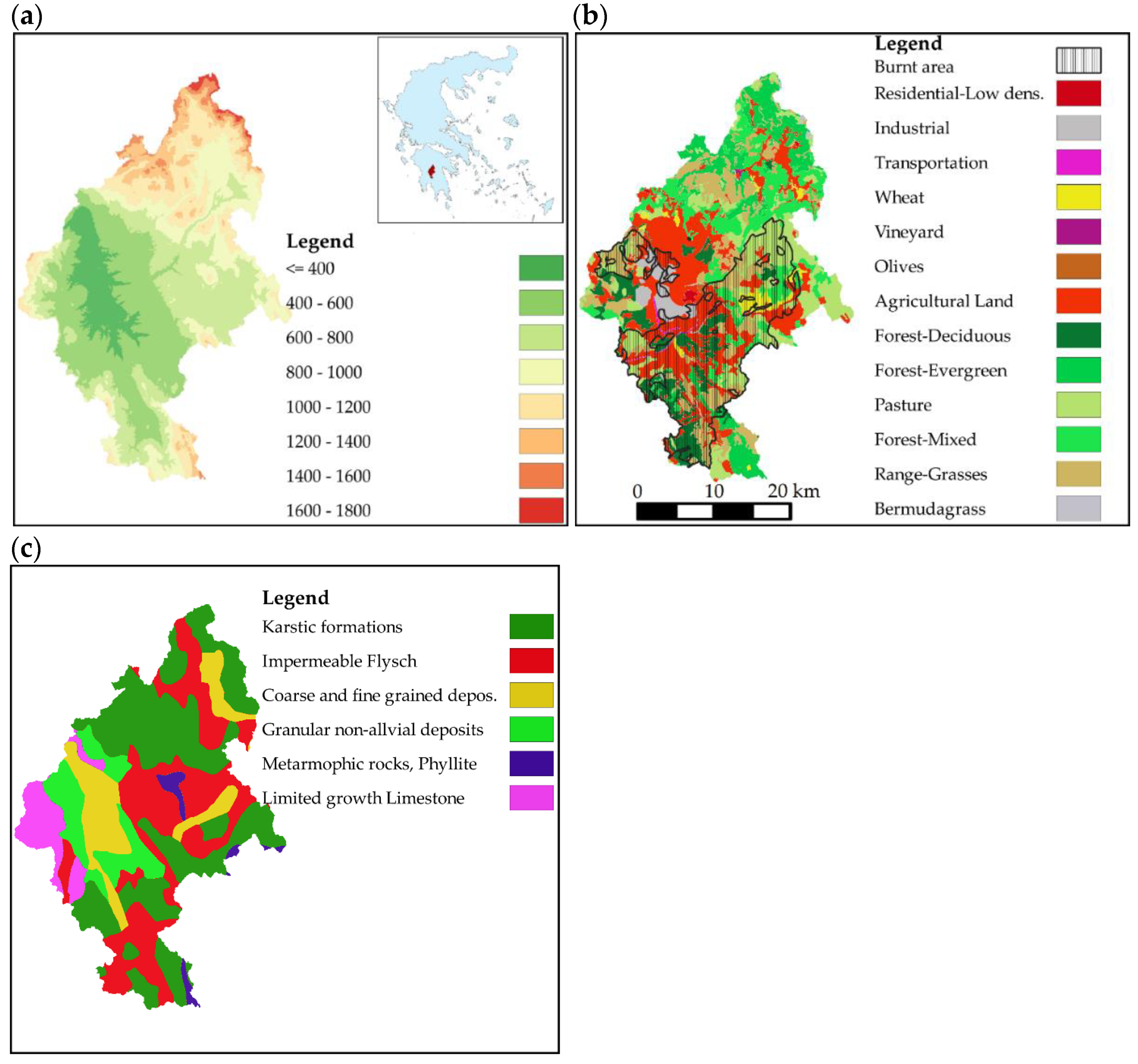
In this study, we examine the hydrological response of the sub-basin upstream of the Karytaina Bridge (37.479448° N, 22.049843° E). The examined river reach is the main one of the Alpheios river. The surface area of the basin is 877 km2, its ground elevation ranges from 272 m to 1878 m with a mean value of 762 m and the length of the main channel is equal to 35.5 km. Information on ground elevation is shown in Figure 1a.
2.4. Data Used
Regarding precipitation, data for the period from 1990–1991 to 2012–2013 are available for 14 stations within and around the basin at the daily time step, and 5 stations at the hourly time step. The double mass curve method is used to verify the statistical homogeneity of annual precipitation depths. Furthermore, a cross correlation test is employed to examine if the stations, especially those outside of the basin, show similar precipitation patterns. This test is necessary because the use of the Thiessen polygon method in the mountainous terrain and microclimatic conditions of the region could severely affect the accuracy of the spatially averaged precipitation depths. Parallel to the Thiessen polygon method, a correction for elevation differences is applied. The rainfall lapse rate is estimated through regressing mean annual precipitation depth on ground elevation for 11 stations. This was found equal to 43.9 mm/100 m. Owing to missing data for some stations, the effective number of stations used to extract the daily time series of precipitation fluctuated between six and twelve.
Potential evapotranspiration is estimated using the Hargreaves method [59]. For this maximum and minimum air temperature data are extracted from two stations (Mornos Dam for the period from October 1990 to September 2002 and Megalopolis from October 2002 to December 2013). The first one of these stations is away from the study basin, but this was the only resort, since there are not air temperature gauges in the area that could cover the period required. The reduction of air temperature with respect to the mean basin elevation is estimated using the values given by Giandotti for Mediterranean catchments South of the 45th parallel. The average daily temperature T is estimated as:
where Tmax and Tmin is the maximum and minimum air temperature respectively.
For the study of the effects of fires on flood discharge, the available data included only one hourly stage time series at the basin outlet, Karytaina Bridge, and hourly rainfall depths from 5 stations within and around the basin for the most significant flood events occurred in the period from 2000 to 2013. Since the lack of precipitation data was frequent, only the events with at least two rain gauges without gaps were considered. The Thiessen polygon method was applied in order to estimate the spatially averaged rainfall. The stages were converted into discharges using the rating curves constructed within the frame of this study.
It should be noted that no significant hydraulic works have been constructed in the test basin. Additionally, due to the use of a rather short data record, the influence of climate change can be considered of minor importance compared to the fire effect. As a result, in this work the separation of the effects of various factors from the fire effect is not considered necessary and is ignored.
The land use data are extracted from maps 1:100,000 of the Corine 2000 project. The main land uses are the cultivated areas and forest areas (deciduous, evergreen and sclerophyllous vegetation) with percentages of area equal to 27.34% and 22.8%, respectively (Figure 1b). Finally, regarding the soil data, the hydro soil map of Greece is used which was developed by the former Hellenic Ministry of Development (Figure 1c). The most prevalent soil type is karstic formations with high values of permeability (39.1% of area) and flysch (29%) which is impermeable. Table 1 presents all the types of soil in the basin with their corresponding hydrologic soil groups and percentages of area within the basin.
3. Results
3.1. Modelling of Daily Streamflow
3.1.1. SWAT—Pre-Fire Period
As mentioned in Section 2, the SWAT model is applied in order to identify differences in the hydrological response of the test basin between the pre-fire and post-fire period. SWAT is calibrated and verified in the pre-fire conditions and then, the knowledge about the basin is used to capture the post-fire regime by modifying only the infiltration mechanism through changing the Curve Number of the SCS method in particular. The aim of this process is to identify how forest fires affect the hydrological variables, both measured (daily, monthly, and annual runoff volume) and unmeasured ones (annual volume of infiltration). The following assumptions are made: (i) the basin is not subdivided into sub-basins but only into 54 HRUs (see description in Section 2.2) using land use, soil type and ground slope as determinants with a threshold of 5% for the percentage of area for each determinant; (ii) the simulation time step is one day.
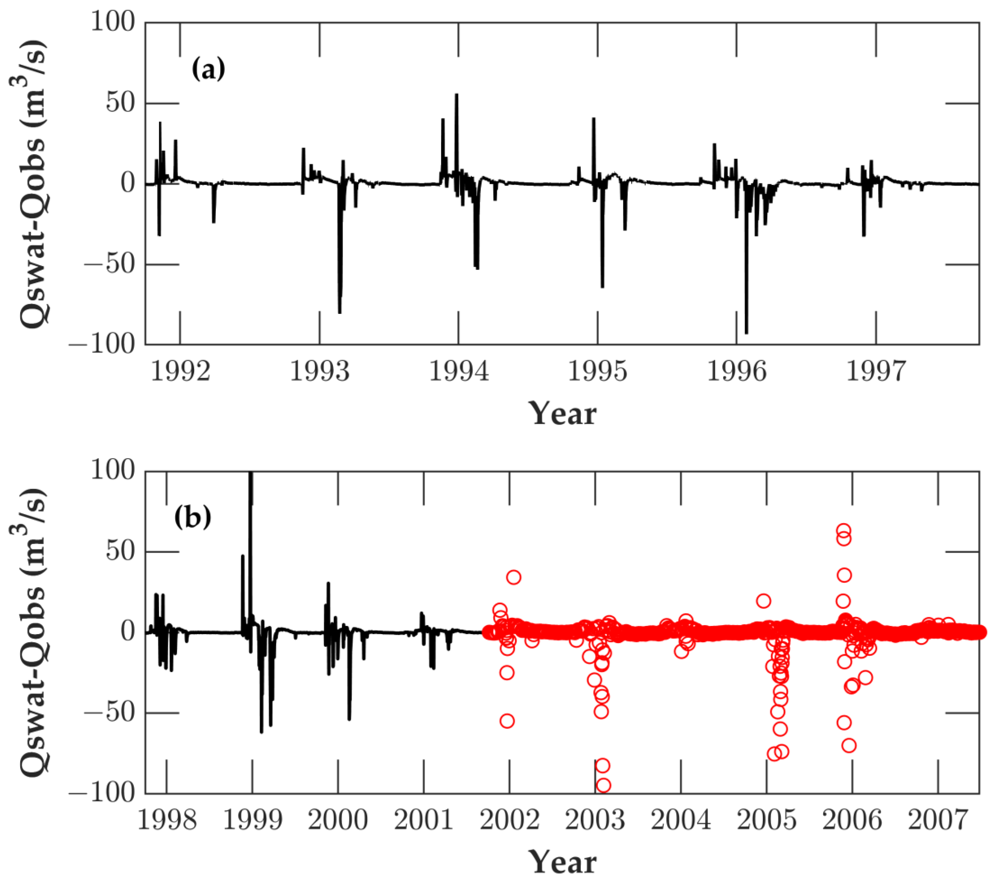
The model is calibrated manually based on mean daily discharge rates for a five-year period (1991–92 to 1996–97). It is noted that the observed daily discharge is obtained through averaging sub-daily values. This was performed by the hydrology section of Public Power Corporation of Greece employing water levels at the two-hour time step converted into discharges using rating curves. The first hydrological year in the data set is used to “warm up” the model. The verification process is based on daily discharge data obtained both from sub-daily values for a four-year period (1997–98 to 2000–01) and stage measurements for the period from 2001–02 to 6/2007. More specifically, for the latter period, instantaneous stage measurements are available, usually in the morning, with a frequency of three measurements per week on average. The stages are converted into discharges via rating curves, which were constructed based on 136 pairs of hydrometric measurements. The Nash-Sutcliffe efficiency is found equal to 0.61 in calibration and 0.71 in verification with model prediction errors (or differences between observed and simulated discharge) depicted in Figure 2a and Figure 2b respectively.
In Table 2, we present the values of Curve Number for normal antecedent moisture conditions (denoted as CNII) for the pre-fire conditions. It should be noted that there are no instances of hydrologic soil type C because there is no such soil type in the basin.
3.1.2. SWAT—Post Fire Period
In order to identify the effect of forest fire on the basin hydrologic regime, it is assumed that only the Curve Number in burnt areas changed after the fire. All the other parameters are assumed to remain unchanged. In general, after the fire, land use in burnt areas is changed from forest areas to some new form of area. Fire severity determines the degree of change, which is usually not homogeneous within a catchment. There are remote sensing methods to identify fire severity [60,61,62], but these were not used in this study. It is assumed that a new land use appears which is termed “burnt areas” and has new characteristics that differ from those of the previous land use but are the same for the same soil type. The new land use is related to a new value for CN. Given that we aim to identify the impact of fires on infiltration for which the SCS-CN method is commonly used, we consider that the above assumption is reasonable.
After the calibration and verification of the model, all the burnt areas are homogenised by adopting a weighted average of the Curve Number for all land uses per soil type for technical reasons. This complies with the above-mentioned assumption about homogeneous fire severity. The average CN can give an idea of the average change in CN in the entire burnt area. In this case, for burnt areas, no distinction of CN is created between land uses, but the values of CN are different for each soil type (Table 2).
By considering the above assumptions regarding CN, we performed two sets of calculations. First, for each hydrological year after the fire, we estimated the differences between the observed and simulated mean annual flow rates by ignoring the change in CN due to fire; the temporal evolution of fire effects is assessed using the Nash–Sutcliffe efficiency per year of the post-fire period. The results confirmed the existing knowledge of the effects of fires. Specifically, by excluding the first year after the fire, the model is found to systematically underestimate the mean annual discharges by 5–22%. Additionally, from Table 3 (fifth column), it is found that ignoring the change in CN due to fire leads to very low values of NSE for the first few years after the fire, while this is gradually improving with time. The weighted average value of CN for the burnt areas was 57.6 in the pre-fire period.
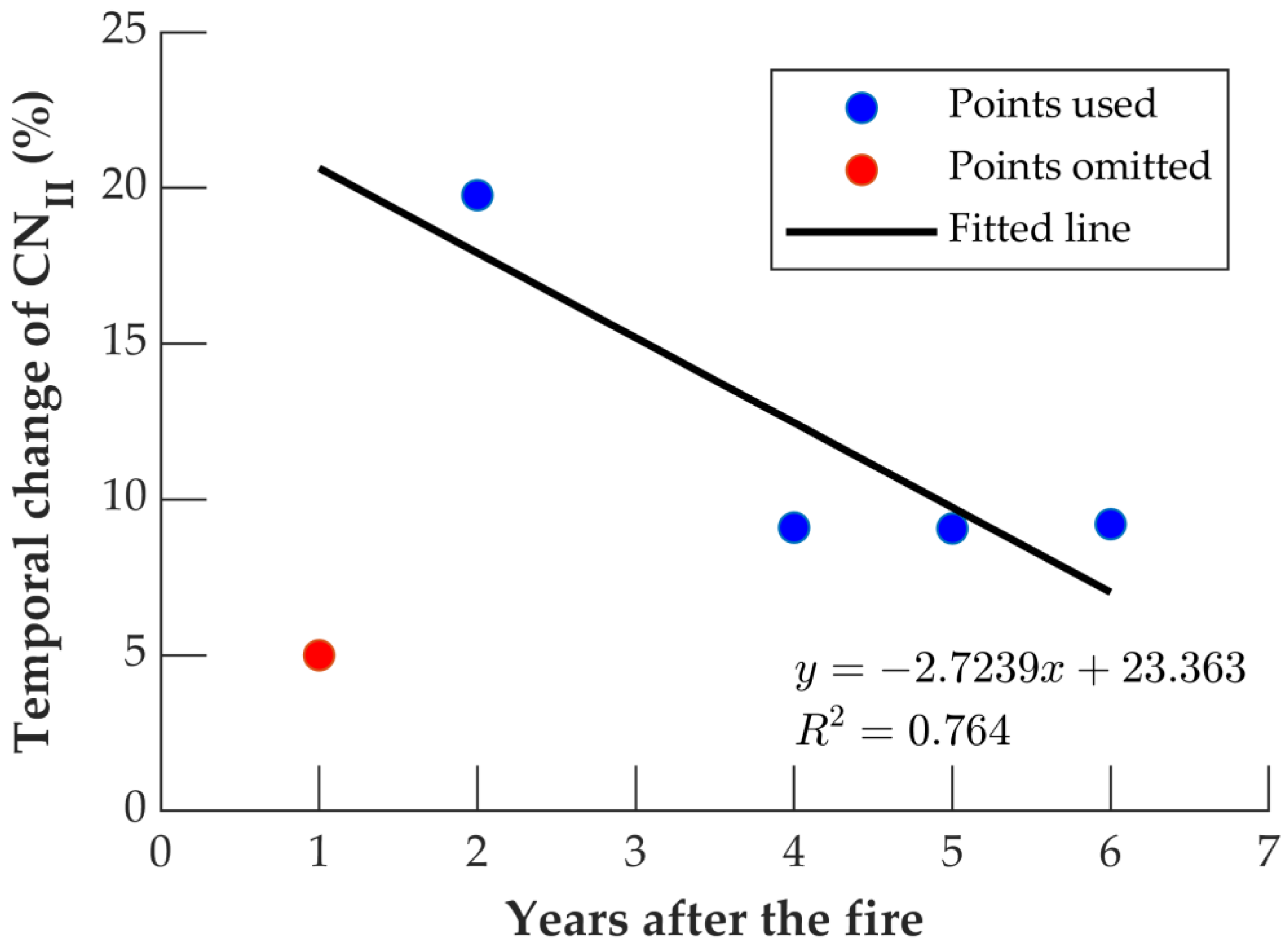
In the second set of calculations, we varied the Curve Number of the burnt areas under normal antecedent moisture conditions (II), i.e., CNIIburnt, with the sole purpose of increasing NSE for each hydrological year. As shown in Table 3, the sixth column, after the fire there is an abrupt increase in CNIIburnt but, thereafter, a gradual decrease follows. Even though the improvement in efficiency is not significant, it seems that an increase in the Curve Number could help better simulate the observed values. The temporal change in CNIIburnt expressed as a percentage of the pre-fire CNII of the same areas is shown in Figure 3. For the first year after the fire, the change was unexpectedly low (5%), while for the third year, this was absolutely unrealistic (−30%). Both estimates correspond to low NSE values and are therefore unreliable. By omitting the first and third years, a linear falling trend in the change in CNIIburnt is found (Figure 3). The rate of fall per year is approximately 2.7%. With regard to the CN changes for the first and third years that are against theory [63], the available information does not allow a safe explanation, but unusual model inputs constitute the most probable cause. It is noteworthy that the first year was very dry. However, the general picture shows an abruptly increased runoff after the fire and then a gradual decrease with time.
3.1.3. Suite of GR Hydrological Models
Three models with different numbers of parameters were used to identify the capability of lumped conceptual models. Maximizing the runoff prediction accuracy was the basis for model construction, while model output variables, such as actual evapotranspiration and percolation, were also examined. The models were calibrated and verified using the same general procedure and performance criterion as in the case of SWAT. The only difference is that, unlike SWAT, these models were calibrated automatically using the Irstea-HBAN procedure [64]. For the pre-fire period, the values of NSE for the calibration of GR4J, GR5J, and GE6J were 0.80, 0.79, and 0.82, respectively. The values for verification were 0.74, 0.69, and 0.78, respectively.
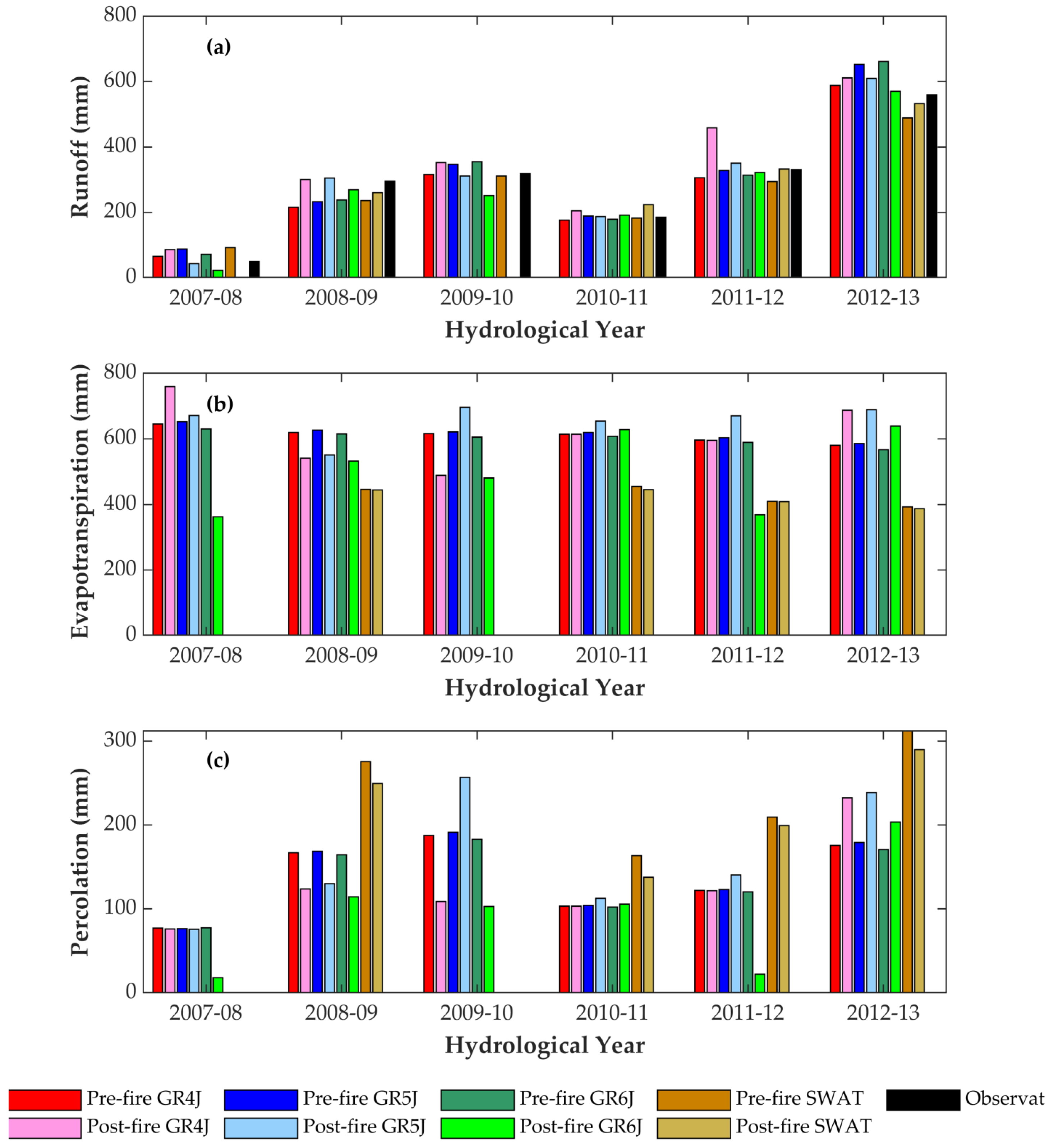
Concerning the post-fire period, model calibration on a year-by-year basis, first the “unconstrained X1” calibrations are performed. High values of NSE were obtained for all models (Table 4), whereas models with pre-fire parameters gave medium to poor NSE. Figure 4 depicts the comparison of water cycle components for each of the three GR models and SWAT using pre-fire parameters and parameters obtained using post-fire data. For SWAT, some years with poor model performance were omitted, as mentioned in Section 3.1.2. As revealed in Figure 4a, there were no large deviations between model runoff predictions. Specifically, all GR models show the same pattern, as pre-fire-based model predictions are consistently above or below post-fire-based model predictions. In general, GR models calibrated for post-fire years predict higher runoff (up to 50%) compared to the predictions of models based on pre-fire years, which is consistent with what is theoretically expected. Yet, for the first year after the fire, which is particularly dry, post-fire-based runoff predictions are approximately 30% lower than those predicted with pre-fire-based models. This shows the high complexity of the studied phenomena and the difficulty in accurately modelling them.
Considering the actual evapotranspiration (Figure 4b), there were two findings. Firstly, for SWAT models, results were very similar between pre-fire and post-fire conditions, which indicates that our choice to change only the Curve Number does not affect evapotranspiration, although some decrease is normally expected. The second finding was that the results of the GR models and pre-fire conditions were consistent with regard to their magnitude. However, when the models were calibrated for the post-fire conditions, a high variability of results rose, which implies that models compensate for the new hydrologic conditions by changing the evapotranspiration along with other variables, without faithfully reproducing real phenomena.
Finally, regarding the percolation (Figure 4c), SWAT predicts decreased values, which is consistent with most studies found in the literature and is theoretically expected from the model structure. GR models predict the same annual volumes for pre-fire-based parameters. However, for post-fire-based models, the percolation volumes are inconsistent: the GR6J model correctly predicts lower percolation for all the years after the fire, whereas GR5J predicts lower percolation for two years only and GR4J for one.
The above inconsistencies led us to resort to the “constrained X1” calibration described in Section 2.2. With the exception of the first year after the fire, using this approach, all models predicted higher simulated runoffs for all the remaining post-fire years as expected (Figure 5a). The value of the NSE (Table 4) was high for all models and practically the same as in the case of “unconstrained X1”. With regard to actual evapotranspiration and percolation, the “constrained X1” post-fire calibration removed inconsistencies (Figure 5b,c).
3.2. Modelling of Flood Events
3.2.1. General
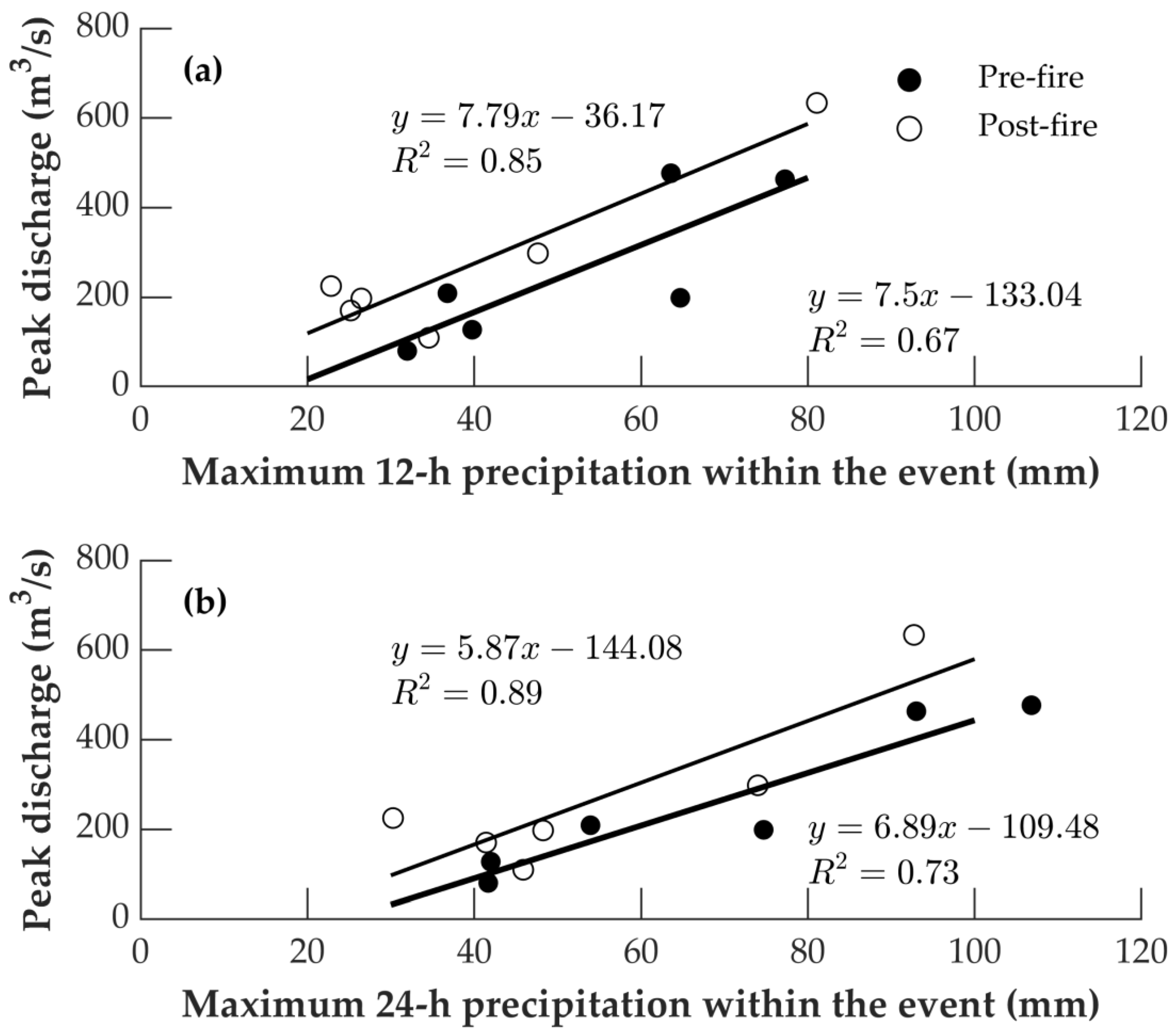
Prior to using HEC-HMS, the time lag, tlag, was estimated as the time interval that maximises the cross-correlation coefficient between rainfall and streamflow series. This quantity is meant to characterise the basin’s response time. The results are shown in Table 5, where we observe that, although tlag before the fire exceeded 10 h for all studied events, the first year after the fire it was diminished to 8 h. However, after the second year, tlag rose again and returned to values similar to those of the pre-fire period. Additionally, we compared the maximum values of the 12 h (Figure 6a) and 24 h rainfall depth (Figure 5b), as obtained from the observed hyetograph, with the maximum observed discharge for each flood event. As expected, events in the post-fire period showed a higher flood peak for the same amount of maximum rainfall. This is revealed by the increasing linear trends presented in Figure 6a,b. It is worth mentioning that the greater the maximum rainfall is, the greater the divergence of flood peaks appears to be between the pre-fire and the post-fire period. The coefficient of determination (R2) was high and statistically significant at the 5% significance level for all linear trend lines fitted. Specifically, for the case with 24 h maximum precipitation, the p-values were 0.00438 and 0.02996 for the pre-fire and post-fire periods, respectively. The corresponding p-values for the case with 12 h maximum precipitation were 0.047 and 0.008517.
3.2.2. Calibration and Verification of the Model in Pre-Fire Conditions
The model HEC-HMS mentioned in the introduction and described in Section 2.1.2 was applied to the data at the hourly time step for the pre-fire period. Before using the model, it was necessary to perform a geomorphological analysis aimed at extracting the necessary information for the model setup. This was implemented using the toolbox HEC-GeoHMS. A Digital Elevation Model (DEM) was used, which had a pixel size of 5.5 m. The DEM was supplied by the National Cadastre and Mapping Agency S.A. of Greece and the geodetic reference system was the European Terrestrial Reference System 1989 (ETRS89), which was converted into the Greek Geodetic Reference System ′87 (GGRS87).
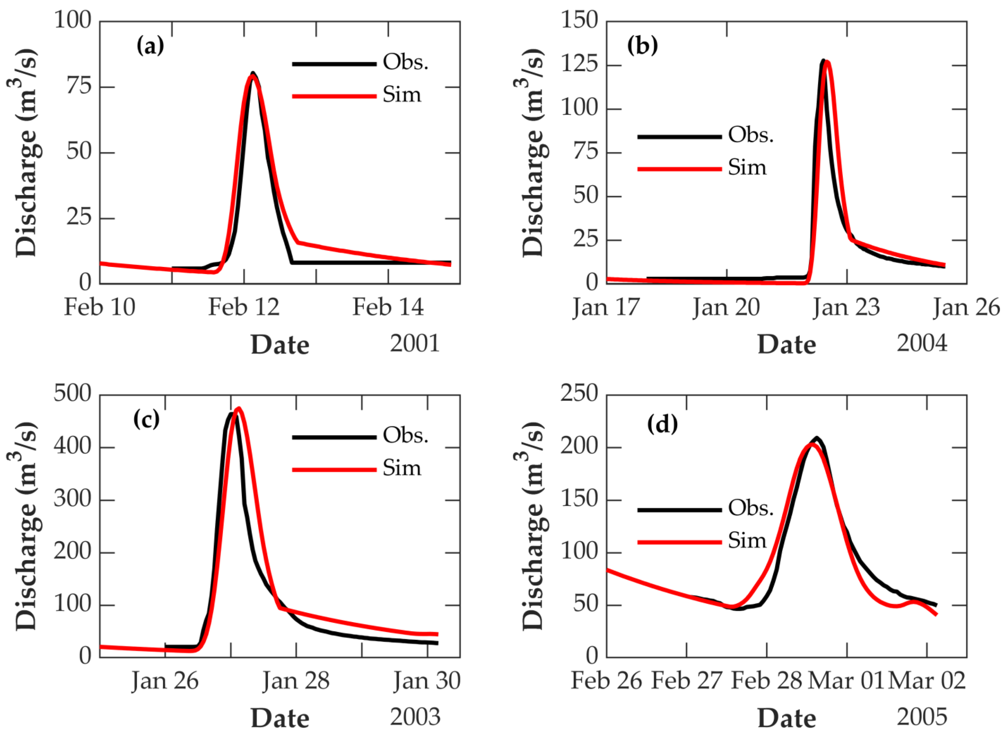
For the calibration and verification of the model, four flood events were used, two of which served for the calibration (2000–01, 2003–04) and two for the verification (2002–03, 2004–05). The SCS-CN method was used as the loss method in all cases. The only parameters that were involved in calibration were the Curve Number, the lag time, and the recession constant of baseflow. Since the aim of this part of the study was to focus on peak flows, the calibration was based on the minimization of the difference between the simulated and observed peak flow rates. In Figure 7, we present the simulated and observed discharge hydrographs for all four events examined. The Curve Number was estimated to be equal to 68.6, the lag time was 600 min (i.e., 10 h), and the recession constant was equal to 0.7. As shown in Table 6, the error in peak flow rate is quite small for the verification period, whereas the flood volume is also well simulated.
3.2.3. On Floods in Post-Fire Conditions
Flood Event in November 2007
In 2007, a major flood occurred for which the only information, apart from hourly precipitation, was the maximum flood stage obtained from the flood trail. This was equal to 10.24 m above the riverbed. The peak discharge was estimated using the rating curve, but the highest measured discharge corresponded to a stage of 5 m. Therefore, the estimated discharge is unknown, which is most probably the reason why the model underestimates the estimated discharge by approximately 10% (Table 7). The flood volume is not presented here, as there was no full discharge hydrograph available.
Flood Event in 9 January 2009–18 January 2009
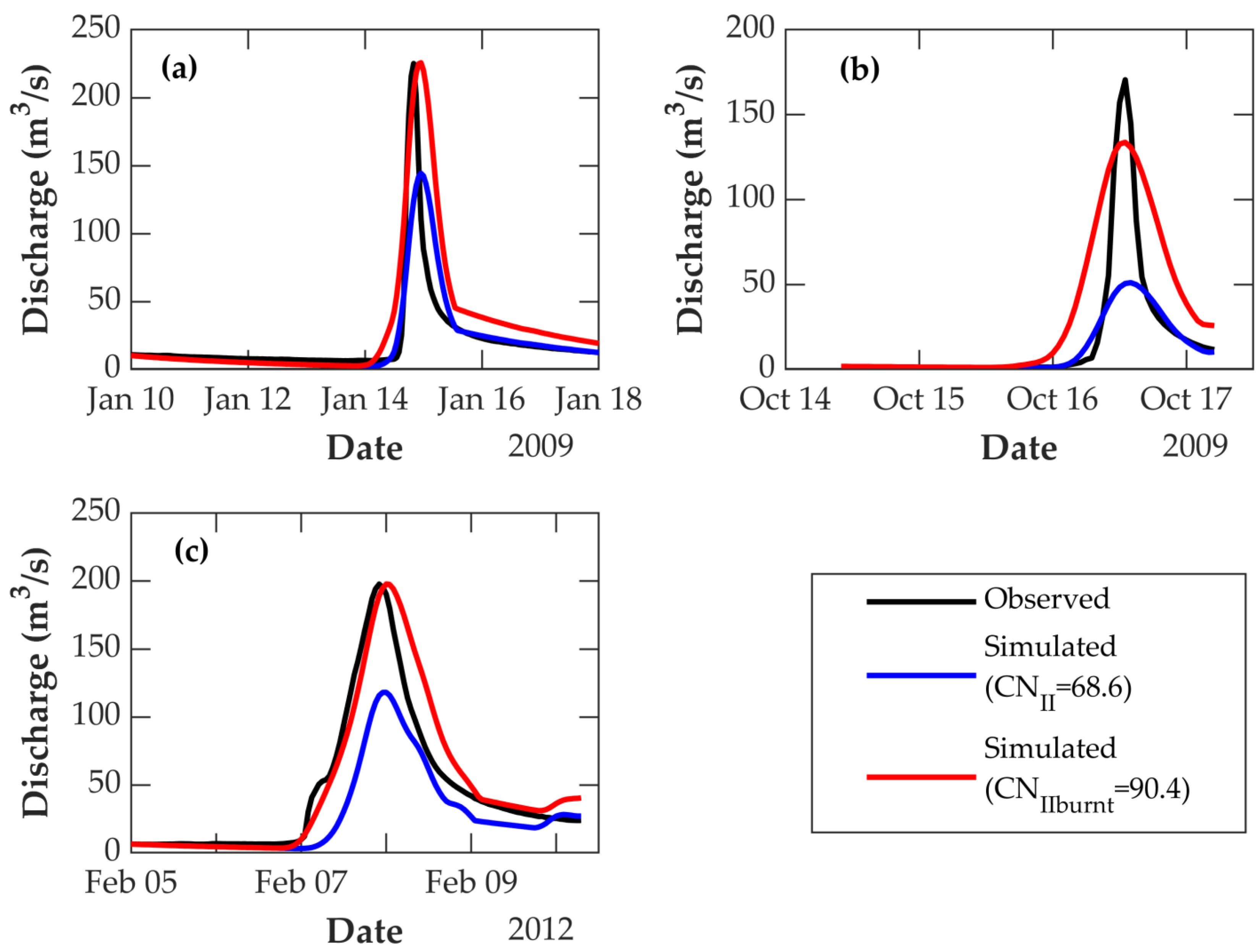
The cumulative precipitation of the five-day period preceding this event was 32.7 mm. According to the SCS-CN method, the CNIII, i.e., CN for wet antecedent moisture conditions, had to be used, which was estimated at 83.4 for the pre-fire period through converting the value of CNII (68.6) into CNIII through Equation (4). For the post-fire period, CNIII was found to be equal to 89.2 and can be converted into CNIIPostFire by inverting Equation (4). Therefore, CNIIPostFire was found to be equal to 78.2 and CNIIBurnt was again equal to 95. In Figure 8a, we depict the simulated hydrographs for the post-fire flood event (for various values of CN) compared to the respective measured ones. It appears that if it is assumed that the hydrological regime did not change after the fire (i.e., CNII = 68.6 for the entire basin), then the model underestimates the peak flow by approximately 36% (Table 7), despite the fact that the model could simulate the slopes of the rising and falling limb of the observed hydrograph satisfactorily. Regarding the flood volume and taking into consideration the change in the Curve Number, the model failed to reproduce it in a satisfactory way because the base length of the simulated hydrograph was wider than that of the observed hydrograph, which apparently helped reproduce the peak flow.
Flood Event in 14 October 2009–17 October 2009
For this flood, the model failed to accurately simulate both the peak flow and flood volume. More specifically, the model underestimated the peak flow by approximately 70%, but when the fire was taken into consideration, the underestimation was only 21.6% (Table 7), although the CNIIBurnt took its maximum value, i.e., 95. From Figure 8b, it becomes obvious that the model inaccurately simulated both the rising and falling limbs of the hydrograph. The cause of this was probably because of an error in the hourly precipitation data, as, for this event, there were only two stations with available data, and one of them was lying outside of the basin.
Flood Event in 5 February 2012–10 February 2012
For the last flood event, the model underestimated the peak flow by 37%. However, when the change in CNII in the burnt areas was taken into consideration, the percent relative error became practically zero. By examining Figure 8c, HEC-HMS seems to describe very well the rising limb and accurately simulate the peak flow. The parameter CNIIBurnt was equal to 90.4. It turns out that CN decreases after some years (here, five years), which is most probably related to the development of the vegetation in the burnt area. As seen in Table 7, for this event, the model could simulate the flood volume fairly well (relative error −9.7%).
Finally, the modified values of the Curve Number were plotted against the date of the occurrence of the related flood event. It appears that, after the third year, CNII began to decrease at a slow rate. However, until the fifth year, the Curve Number still remained above 90. A second-order polynomial fit to this trend is shown in Figure 9. It is noted that all values of the Curve Number after the first year belong to the falling limb of the fitted polynomial, as expected from the anticipated recovery of vegetation, and, in general, land use changes after the fire.
3.3. Comparing Results at the Two Timescales
This study showed that after the fire, the Curve Number of burnt areas increases in both timescales. The magnitude of change is, however, different from one timescale to another. This is because SWAT is a continuous-time model that modifies CN in dry periods, whereas HEC-RAS is an event-based model that keeps CN constant in time. Moreover, the inaccuracy in the representation of flood processes when using a daily time step, superimposed on other sources of error, can justify the differences in CN values, at least in part. Moreover, it appears that there is a high linear correlation between the CN values on the two timescales. More specifically, after plotting the values of CNII for the two timescales against time expressed in years after the fire and fitting a linear trend line, the cross-correlation of the predicted values through these trend lines is found to be high. The two linear trend lines shown in Figure 10 have slopes that are statistically significant at approximately the 10% significance level. We adopted the 10% significance level, i.e., the maximum acceptable value, because of the high uncertainty of factors involved in the analysis. Contrary to the absolute values of the two slopes, the slope difference is statistically insignificant. This implies that the rate of decrease is statistically the same for both timescales. Conversely, the intercepts of the two lines are significant at a very low significance level (below 0.01) and the same holds for their difference. The latter implies a systematic deviation between the Curve Numbers for the two timescales, with the hourly scale showing larger values by approximately 40%.
4. Discussion
A large-scale forest fire affects many components of the water cycle, such as evapotranspiration, infiltration, and runoff. Furthermore, it changes the land use, increases erosion, and can create a water-repellent soil layer. In recent years, the issue of change has become of major importance for the hydrological sciences. The scientific initiative of the International Association of Hydrological Sciences (IAHS) for the decade 2013–2022, entitled “Panta Rhei-Everything Flows” [65], aims at making predictions of water resource dynamics in a changing environment. The key questions are: (i) how we can identify hydrological changes; (ii) what is the amount of data required for the identification of the potential impact of catchment changes; (iii) is the use of models necessary for such identification and, if so, what type of models are preferred.
It is widely accepted that all models suffer from various kinds of uncertainty, such as data uncertainty, parameter estimation uncertainty, model structural uncertainty, and perceptual model uncertainty [66]. Those uncertainties, superimposed on model equifinality, create models that may not be able to inform us about a change. This has been expressed by George Box [67] in his quote: “All models are wrong, but some models are useful”. There are methodologies that employ only observed data to identify a change. These cannot, however, identify the cause of change, nor can they help acquire in-depth knowledge about the processes involved. Usually, the selection of a model is based on the goal of the study, data availability, and prior experience with the use of a specific model.
In this study, after 2001, there were no observed daily discharges available, but only measurements with a frequency of one every two or three days. This rendered the use of models inevitable. We selected a wide spectrum of models, from semi-distributed (SWAT and HEC-HMS) to lumped (GR4J, GR5J, and GR6J) and from models using the SCS-CN method for the estimation of infiltration (SWAT and HEC-HMS) to simple conceptual models with four to six parameters (GR models).
The comparison of our results with results from the literature reveals that our results are consistent with most of the existing studies. Considering flood events at the hourly time-step, Cydzik and Hogue [26] calculated the post-fire CN to be approximately 85 for the first year, while the pre-fire value was approximately 57. The CN almost reached its pre-fire values after three years. Lag time decreased from 2 h to 1.5 h for the three years after the fire. Papathanasiou et al. [28] found CN to increase for two sub-basins from 40 and 45 to 82 and 79, respectively. The lag time decreased for the first sub-basin from 2 h to 1.5 h, whereas in the other sub-basin, lag time was not affected. McLin et al. [30] found a strong correlation between the relative increase in CN and the relative decrease in lag time for the post-fire condition. The change for both variables was from 0 to 75%. The Burned Area Emergency Rehabilitation team, BAER, [68] assigned CN values equal to 65, 85, and 90 for low, medium, and high severity burnt areas, respectively. For the daily time step, Havel et al. [31] estimated the increase in CN to be approximately 5, 10, and 15 for low, medium, and high-burnt severity.
With regard to the first research question set in the introduction, our modelling effort using a variety of models revealed that the daily runoff volume and hourly peak discharge are severely underestimated for the post-fire period if no model recalibration is performed. The percent underestimation is in the order of more than 20% and 30% for the daily and hourly timescales, respectively. The lack of measurements for other variables, such as percolation, combined with the large scale of the fire phenomena and model equifinality, prevented us from drawing safe conclusions about variables other than runoff. Regarding the temporal evolution of model parameters in the post-fire period we recall that parameter combinations that would allow for gradual runoff decrease were naturally expected. Indeed, we have been able to verify such behaviour for SWAT and HEC-HMS, despite the high complexity of hydrological processes due to the spatial extent of the study basin. Of course, this was achieved through confining the recalibration parameter set to only one parameter, i.e., the Curve Number. Moreover, the rate of post-fire fall of the Curve Number proved to be independent of the timescale. This timescale invariance is certainly promising for future modelling methodologies.
Regarding the second question, our search of the literature revealed that the existing knowledge on fire effects in small basins is far from sufficient for the prediction of runoff in large basins using semi-distributed hydrological models. For such a prediction, the small test basin should be similar to the modelled unit of the semi-distributed model in many respects, namely, its topography, soil, vegetation, climatology, burn severity, and fire extent, to mention only a few. It goes without saying that the results from the experimental basins would be more desirable than any model predictions. Unfortunately, experimental basins are small in size, and their measurements are very unlikely to cover the whole spectrum of the required information for a large basin. In the case of lumped models, it becomes impracticable to exploit the above-mentioned idea of basin similarity, and, hence, the model calibration exercise remains the only alternative. Some of our tests with lumped models revealed some inconsistencies in the fire effect on processes other than runoff, the latter being the only variable involved in model calibration and, consequently, being forced to be consistent with measurements.
Although no wide consensus has been established with regard to the questions posed in this work, we believe that there is a favorable perspective for this, which is justified by the recent intensification of related research efforts worldwide (e.g., [69,70,71,72], to mention but a few.) Additionally, one should not lose sight of the fact that many anthropogenic influences act simultaneously (e.g., forest fires, deforestation, large-scale hydraulic works) and affect the same hydrological variables by: (i) altering the rate of evaporation, (ii) modifying the velocity and amount of overland flow, (iii) altering the amount of infiltration into the ground, and (iv) affecting the amount of intercepted water [73].
The issue of the identification of the best model features remains open, and models that are different from those used in this work would merit further study, e.g., Hydrologiska Byråns Vattenavdelning (HBV) [74], SACRAMENTO [75], Australian Water Balance Model (AWBM) [76], and Hydrological Model Focusing on Sub-Flows Variation (HMSV) [77]. On top of that, the choice of model performance measure induces some uncertainty. In this work, only NSE was employed, although other measures could also be used [78,79,80].
5. Conclusions
In this paper, the hydrologic effects of a large-scale forest fire were investigated using five models, namely SWAT, GR4J, GR5J, GR6J, and HEC-HMS. The use of the models proved useful in extracting information that could not otherwise be extracted. With respect to the spatial variability of modelled processes, the selected models cover a wide spectrum, i.e., from lumped models of the GR model suite to semi-distributed models SWAT and HEC-HMS. Regarding the mathematical representation of processes, SWAT and HEC-HMS implement the SCS-CN method, whereas the GR Suite models employ a different modelling approach. With regard to the employed time step, four models (SWAT, GR3J, GR4J, and GR5J) used the daily time step, whereas HEC-HMS was run at the hourly time step.
The results of our investigation allow us to draw the following conclusions:
- For both the daily and hourly time steps, there was a significant increase in the Curve Number after the fire was found.
- For daily streamflow, the SWAT model gave low values of the Nash–Sutcliffe efficiency when applied to the post-fire period, after it had been calibrated and verified for the pre-fire period. However, an increase in the Curve Number by approximately 20% clearly improved the NSE for the post-fire period. The Curve Number showed a decreasing trend with respect to time after the fire, which is consistent with the presumed regeneration of the vegetation. It appeared that, when used without recalibration after the fire, the SWAT model underestimates the daily streamflow by approximately 22% on average.
- For the hourly time step study using the HEC-HMS model, the threshold of the Curve Number in burnt areas was set to 95. The results showed that for a period of approximately three years after the fire, the Curve Number was still 95 in the burnt areas during the flood events, with a slow decrease rate after the third year. However, until the fifth year, the Curve Number still remained above 90. The model underestimated the peak flow in the basin by 35–70% (60 m3/s to 300 m3/s in absolute values), whereas the model proved capable of simulating the post-fire flood events in a satisfactory way if the modeller has knowledge about the change in Curve Number due to fire.
- The linear trend lines of the Curve Number in burnt areas with respect to time for the two-timescales show the same slope but different intercepts, with the latter being larger for the hourly scale. This implies that the magnitude of the Curve Number is systematically higher in the case of the hourly time step, but its rate of temporal decrease is timescale-independent.
- Past findings suggest that the hydrologic effects of a forest fire can be highly variable and difficulties in the model were verified in this study; specifically, in the first year after the fire, which was particularly dry, all models faced difficulties, which revealed that a unique model structure, such as that of the selected models, may not be sufficient.
- The lumped models employed in this work for daily simulations (GR Suite) showed very high performance with respect to the accuracy of prediction of the observed streamflow. Their credibility in predicting post-fire hydrological variables other than runoff was found to be considerably enhanced by employing parameter constraints in calibration. In this work, the use of the pre-fire value of parameter X1 (runoff production store capacity) as the upper bound in post-fire calibration proved particularly useful for a realistic simulation of internal model variables, such as actual evapotranspiration and percolation.
Author Contributions
Conceptualization, I.N. and S.C.B.; methodology, I.N. and S.C.B.; software, S.C.B.; validation, S.C.B. and I.N.; formal analysis, I.N. and S.C.B.; investigation, S.C.B.; data curation, S.C.B.; writing—original draft preparation, S.C.B. and I.N.; writing—review and editing, I.N. and S.C.B.; visualization, I.N. and S.C.B.; supervision, I.N. All authors have read and agreed to the published version of the manuscript.
Funding
This research received no external funding.
Institutional Review Board Statement
Not applicable.
Informed Consent Statement
Not applicable.
Data Availability Statement
Hydrological and geospatial data are available on request from the Public Power Corporation of Greece and the National Cadastre and Mapping Agency S.A. of Greece, respectively.
Acknowledgments
The authors would like to express their gratitude to I. Kouvopoulos from the Public Power Corporation of Greece, as well as other members of staff of the corporation, for their kind supply of data for discharge and precipitation.
Conflicts of Interest
The authors declare no conflict of interest.
References
- Rycroft, H.B. A Note on the Immediate Effects of Veldburning on Stormflow in a Jonkershoek Stream Catchment. J. S. Afr. For. Assoc. 1947, 15, 80–88. [Google Scholar] [CrossRef]
- Colman, C.A. Fire and water in southern California’s mountains. Calif. For. Range Exp. Stn. Misc. Pap. 1953, 3, 1–8. [Google Scholar]
- Lavabre, J.; Torres, D.S.; Cernesson, F. Changes in the hydrological response of a small Mediterranean basin a year after a wildfire. J. Hydrol. 1993, 142, 273–299. [Google Scholar] [CrossRef]
- Townsend, S.A.; Douglas, M.M. The effect of three fire regimes on stream water quality, water yield and export coefficients in a tropical savanna (northern Australia). J. Hydrol. 2000, 229, 118–137. [Google Scholar] [CrossRef]
- Pierson, F.B.; Robichaud, P.R.; Spaeth, K.E. Spatial and temporal effects of wildfire on the hydrology of a steep rangeland watershed. Hydrol. Process. 2001, 15, 2905–2916. [Google Scholar] [CrossRef]
- Springer, E.P.; Hawkins, R.H. Curve number and peakflow responses following the Cerro Grande fire on a small watershed. In Proceedings of the Watershed Management Conference “Managing Watersheds for Human and Natural Impacts Engineering, Ecological and Economic Challenges”, Williamsburg, VA, USA, 19–22 July 2005. [Google Scholar]
- Shakesby, R.A.; Doerr, S.H. Wildfire as a hydrological and geomorphological agent. Earth-Sci. Rev. 2006, 74, 269–307. [Google Scholar] [CrossRef]
- Lane, P.N.; Sheridan, G.J.; Noske, P.J. Changes in sediment loads and discharge from small mountain catchments following wildfire in south eastern Australia. J. Hydrol. 2006, 331, 495–510. [Google Scholar] [CrossRef]
- Moody, J.A.; Martin, D.A. Initial hydrologic and geomorphic response following a wildfire in the Colorado Front Range. Earth Surf. Process. Landf. 2001, 26, 1049–1070. [Google Scholar] [CrossRef]
- Moody, J.A.; Martin, D.A.; Haire, S.L.; Kinner, D.A. Linking runoff response to burn severity after a wildfire. Hydrol. Process. 2008, 22, 2063–2074. [Google Scholar] [CrossRef]
- Stoof, C.R.; Vervoort, R.W.; Iwema, J.; van den Elsen, E.; Ferreira, A.J.D.; Ritsema, C.J. Hydrological response of a small catchment burned by experimental fire. Hydrol. Earth Syst. Sci. 2012, 16, 267–285. [Google Scholar] [CrossRef] [Green Version]
- Scott, D.F.; Van Wyk, D.B. The effects of wildfire on soil wettability and hydrological behaviour of an afforested catchment. J. Hydrol. 1990, 121, 239–256. [Google Scholar] [CrossRef]
- Scott, D.F. The hydrological effects of fire in South African mountain catchments. J. Hydrol. 1993, 150, 409–432. [Google Scholar] [CrossRef] [Green Version]
- Soler, M.; Sala, M.; Gallart, F. Post fire evolution of runoff and erosion during an eighteen month period. Soil erosion and degradation as a consequence of forest fires. In Soil Degradation and Desertification in Mediterranean Environments; Sala, M., Rubio, J.L., Eds.; Geoforma Ediciones: Logroño, Spain, 1994; pp. 149–161. [Google Scholar]
- Soto, B.; Basanta, R.; Benito, E.; Perez, R.; Diaz-Fierros, F. Runoff and erosion from burnt soils in northwest Spain. Soil Erosion as a consequence of forest fires. In Soil Degradation and Desertification in Mediterranean Environments; Sala, M., Rubio, J.L., Eds.; Geoforma Ediciones: Logroño, Spain, 1994; pp. 91–98. [Google Scholar]
- Mayor, A.G.; Bautista, S.; Llovet, J.; Bellot, J. Post-fire hydrological and erosional responses of a Mediterranean landscape: Seven years of catchment-scale dynamics. Catena 2007, 71, 68–75. [Google Scholar] [CrossRef]
- Bart, R.; Hope, A. Streamflow response to fire in large catchments of a Mediterranean-climate region using paired-catchment experiments. J. Hydrol. 2010, 388, 370–378. [Google Scholar] [CrossRef]
- Inbar, M.; Tamir, M.; Wittenberg, L. Runoff and erosion processes after a forest fire in Mount Carmel, a Mediterranean area. Geomorphol. 1998, 24, 17–33. [Google Scholar] [CrossRef]
- Rulli, M.C.; Rosso, R. Hydrologic response of upland catchments to wildfires. Adv. Water Resour. 2007, 30, 2072–2086. [Google Scholar] [CrossRef]
- Cerrelli, G.A. FIRE HYDRO, a simplified method for predicting peak discharges to assist in the design of flood protection measures for western wildfires. In Proceedings of the Watershed Management Conference “Managing Watersheds for Human and Natural Impacts Engineering, Ecological and Economic Challenges”, Williamsburg, VA, USA, 19–22 July 2005. [Google Scholar]
- Feikema, P.M.; Sherwin, C.B.; Lane, P.N. Influence of climate, fire severity and forest mortality on predictions of long term streamflow: Potential effect of the 2009 wildfire on Melbourne’s water supply catchments. J. Hydrol. 2013, 488, 1–16. [Google Scholar] [CrossRef]
- Batelis, S.C.; Nalbantis, I. Potential effects of forest fires on streamflow in the Enipeas river basin, Thessaly, Greece. Environ. Process. 2014, 1, 73–85. [Google Scholar] [CrossRef] [Green Version]
- Versini, P.A.; Velasco, M.; Cabello, A.; Sempere-Torres, D. Hydrological impact of forest fires and climate change in a Mediterranean basin. Nat. Hazards 2013, 66, 609–628. [Google Scholar] [CrossRef]
- Earles, T.A.; Wright, K.R.; Brown, C.; Langan, T.E. Los Alamos forest fire impact modelling. J. Am. Water Resour. Assoc. 2004, 40, 371–384. [Google Scholar] [CrossRef]
- Goodrich, D.C.; Canfield, H.E.; Burns, I.S.; Semmens, D.J.; Miller, S.N.; Hernandez, M.; Levick, L.R.; Guertin, D.P.; Kepner, W.G. Rapid post-fire hydrologic watershed assessment using the AGWA GIS-based hydrologic modeling tool. In Proceedings of the Watershed Management Conference “Managing Watersheds for Human and Natural Impacts Engineering, Ecological and Economic Challenges”, Williamsburg, VA, USA, 19–22 July 2005. [Google Scholar]
- Cydzik, K.; Hogue, T.S. Modeling Postfire Response and Recovery using the Hydrologic Engineering Center Hydrologic Modeling System (HEC-HMS). J. Am. Water Resour. Assoc. 2009, 45, 702–714. [Google Scholar] [CrossRef]
- Nalbantis, I.; Lymperopoulos, S. Assessment of flood frequency after forest fires in small ungauged basins based on uncertain measurements. Hydrol. Sci. J. 2012, 57, 52–72. [Google Scholar] [CrossRef]
- Papathanasiou, C.; Alonistioti, D.; Kasella, A.; Makropoulos, C.; Mimikou, M. The impact of forest fires on the vulnerability of peri-urban catchments to flood events (The case of the Eastern Attica Region). Glob. NEST 2012, 14, 294–302. [Google Scholar]
- Papathanasiou, C.; Makropoulos, C.; Mimikou, M. Hydrological modelling for flood forecasting: Calibrating the post-fire initial conditions. J. Hydrol. 2015, 529, 1838–1850. [Google Scholar] [CrossRef]
- McLin, S.G.; Springer, E.P.; Lane, L.J. Predicting floodplain boundary changes following the Cerro Grande wildfire. Hydrol. Process. 2001, 15, 2967–2980. [Google Scholar] [CrossRef]
- Havel, A.; Tasdighi, A.; Arabi, M. Assessing the hydrologic response to wildfires in mountainous regions. Hydrol. Earth Syst. Sci. 2017, 22, 2527–2550. [Google Scholar] [CrossRef] [Green Version]
- NRCS. Hydrologic Soil Cover Complexes. In National Engineering Manual; USDA Natural Resources Conservation Service; NRCS: Washington, DC, USA, 2004; Chapter 9; p. 210-VI-NEH. [Google Scholar]
- Bertalanffy Von, L. General Systems Theory; Braziller: New York, NY, USA, 1962. [Google Scholar]
- Beven, K.J.; Freer, J. Equifinality, data assimilation, and uncertainty estimation in mechanistic modelling of complex environmental systems. J. Hydrol. 2001, 249, 11–29. [Google Scholar] [CrossRef]
- Arnold, J.G.; Williams, J.R.; Srinivasan, R.; King, K.W. SWAT: Soil and Water Assessment Tool; US Department of Agriculture, Agricultural Research Service: Temple, TX, USA, 1999.
- Neitsch, S.L.; Arnold, J.G.; Williams, J.R. Soil and Water Assessment Tool User’s Manual; US Department of Agriculture, Agricultural Research Service: Temple, TX, USA, 1999.
- Neitsch, S.L.; Arnold, J.G.; Kiniry, G.R.; Williams, J.R. Soil and Water Assessment Theoretical Tool Documentation; US Department of Agriculture, Agricultural Research Service: Temple, TX, USA, 2005.
- Bladon, K.D.; Silins, U.; Emelko, M.B.; Flannigan, M.; Dupont, D.; Robinne, F.; Wang, X.; Parisien, M.A.; Stone, M.; Thompson, D.K.; et al. Assessing the Impact of Active Land Management in Mitigating Wildfire Threat to Source Water Supply Quality; AGU Fall Meeting Abstracts: Washington, DC, USA, 2014; Volume 1, p. 4. [Google Scholar]
- Havel, A. Hydrologic and Hydraulic Response to Wildfires in the Upper Cache la Poudre Watershed Using a SWAT and HEC-RAS Model Cascade. Ph.D. Thesis, Colorado State University, Fort Collins, CO, USA, 2016. [Google Scholar]
- Liu, J.; Paul, S.; Manguerra, H. ArcSWAT Modeling Analysis for Post-Wildfire Logging Impacts on Sediment and Water Yields at Salmon-Challis National Forest, Idaho, USA. In Proceedings of the Watershed Management 2015 Symposium, Reston, VA, USA, 5–7 August 2015; pp. 240–250. [Google Scholar]
- Narsimlu, B.; Gosain, A.K.; Chahar, B.R.; Singh, S.K.; Srivastava, P.K. SWAT model calibration and uncertainty analysis for streamflow prediction in the Kunwari River Basin, India, using sequential uncertainty fitting. Environ. Process. 2015, 2, 79–95. [Google Scholar] [CrossRef]
- Putz, G.; Burke, J.M.; Smith, D.W.; Chanasyk, D.S.; Prepas, E.E.; Mapfumo, E. Modelling the effects of boreal forest landscape management upon streamflow and water quality: Basic concepts and considerations. J. Environ. Eng. Sci. 2003, 2, S87–S101. [Google Scholar] [CrossRef]
- Stengel, V.G. Comparing Simulated Hydrologic Response Before and After the 2011 Bastrop Complex Wildfire. Ph.D. Thesis, Texas State University, San Marcos, TX, USA, 2014. [Google Scholar]
- Watson, F.G. Large Scale, Long Term, Physically Based Modelling of the Effects of Land Cover Change on Forest Water Yield. Ph.D. Thesis, University of Melbourne, Melbourne, Australia, 1999. [Google Scholar]
- Goswami, M.; O’Connor, K.M.; Bhattarai, K.P. Development of regionalisation procedures using a multi-model approach for flow simulation in an ungauged catchment. J. Hydrol. 2007, 333, 517–531. [Google Scholar] [CrossRef]
- Sivapalan, M.; Takeuchi, K.; Franks, S.W.; Gupta, V.K.; Karambiri, H.; Lakshmi, V.; Liang, X.; McDonnell, J.J.; Mendiondo, E.M.; O’Connell, P.E.; et al. IAHS Decade on Predictions in Ungauged Basins (PUB), 2003–2012: Shaping an exciting future for the hydrological sciences. Hydrol. Sci. J. 2003, 48, 857–880. [Google Scholar] [CrossRef] [Green Version]
- Watson, F.G.; Vertessy, R.A.; Grayson, R.B. Large-scale modelling of forest hydrological processes and their long-term effect on water yield. Hydrol. Process. 1999, 13, 689–700. [Google Scholar] [CrossRef]
- Lane, P.N.; Feikema, P.M.; Sherwin, C.B.; Peel, M.C.; Freebairn, A.C. Modelling the long term water yield impact of wildfire and other forest disturbance in Eucalypt forests. Environ. Model. Softw. 2010, 25, 467–478. [Google Scholar] [CrossRef]
- Zhou, Y.; Zhang, Y.; Vaze, J.; Lane, P.; Xu, S. Improving runoff estimates using remote sensing vegetation data for bushfire impacted catchments. Agr. For. Meteorol. 2013, 182, 332–341. [Google Scholar] [CrossRef]
- Zhou, Y.; Zhang, Y.; Vaze, J.; Lane, P.; Xu, S. Impact of bushfire and climate variability on streamflow from forested catchments in southeast Australia. Hydrol. Sci. J. 2015, 60, 1340–1360. [Google Scholar] [CrossRef] [Green Version]
- US Army Corps of Engineers Hydrologic Engineering Center. Hydrologic Modeling System. In HEC-HMS User’s Manual; Hydrologic Engineering Center: Davis, CA, USA, 2015. [Google Scholar]
- DeBano, L.F. The role of fire and soil heating on water repellency in wildland environments: A review. J. Hydrol. 2000, 231, 195–206. [Google Scholar] [CrossRef]
- Perrin, C.; Michel, C.; Andréassian, V. Improvement of a parsimonious model for streamflow simulation. J. Hydrol. 2003, 279, 275–289. [Google Scholar] [CrossRef]
- Le Moine, N. Le Bassin Versant de Surface vu Par le Souterrain: Une Voie D’amélioration des Performances et du Réalisme des Modèles Pluie-débit? Ph.D. Thesis, University Paris 6, Paris, France, 2008. [Google Scholar]
- Pushpalatha, R.; Perrin, C.; Le Moine, N.; Mathevet, T.; Andréassian, V. A downward structural sensitivity analysis of hydrological models to improve low-flow simulation. J. Hydrol. 2011, 411, 66–76. [Google Scholar] [CrossRef]
- Nash, J.; Sutcliffe, J.V. River flow forecasting through conceptual models part I—A discussion of principles. J. Hydrol. 1970, 10, 282–290. [Google Scholar] [CrossRef]
- Chow, V.T.; Maidment, D.R.; Mays, L.W. Applied Hydrology; McGraw-Hill: New York, NY, USA, 1988. [Google Scholar]
- WWF. Ecological Assessment of the Wildfires of August 2007 in the Peloponnese; World Wide Fund: Greece, Athens, 2007. [Google Scholar]
- Hargreaves, G.H.; Samani, Z.A. Reference crop evapotranspiration from ambient air temperature. Am. Soc. Agric. Eng. 1985, 1, 96–99. [Google Scholar] [CrossRef]
- Roy, D.P.; Boschetti, L.; Trigg, S.N. Remote sensing of fire severity: Assessing the performance of the normalized burn ratio. IEEE Geosci. Remote Sens. Lett. 2006, 3, 112–116. [Google Scholar] [CrossRef] [Green Version]
- Escuin, S.; Navarro, R.; Fernandez, P. Fire severity assessment by using NBR (Normalized Burn Ratio) and NDVI (Normalized Difference Vegetation Index) derived from LANDSAT TM/ETM images. Int. J. Remote Sens. 2008, 29, 1053–1073. [Google Scholar] [CrossRef]
- Keeley, J.E. Fire intensity, fire severity and burn severity: A brief review and suggested usage. Int. J. Wildland Fire 2009, 18, 116–126. [Google Scholar] [CrossRef]
- Saxe, S.; Hogue, T.S.; Hay, L. Characterization and evaluation of controls on post-fire streamflow response across western US watersheds. Hydrol. Earth Syst. Sci. 2018, 22, 1221–1237. [Google Scholar] [CrossRef] [Green Version]
- Michel, C. Hydrologie appliquée aux petits bassins ruraux. In Hydrology Handbook; Cemagref: Anthony, France, 1991. (In French) [Google Scholar]
- Montanari, A.; Young, G.; Savenije, H.H.G.; Hughes, D.; Wagener, T.; Ren, L.L.; Koutsoyiannis, D.; Cudennec, C.; Toth, E.; Grimaldi, S.; et al. “Panta Rhei—Everything flows”: Change in hydrology and society—The IAHS scientific decade 2013–2022. Hydrol. Sci. J. 2013, 58, 1256–1275. [Google Scholar] [CrossRef]
- Wagener, T.; Gupta, H.V. Model identification for hydrological forecasting under uncertainty. Stoch. Environ. Res. Risk Assess. 2005, 19, 378–387. [Google Scholar] [CrossRef]
- Box, G.E. Science and statistics. J. Am. Stat. Assoc. 1976, 71, 791–799. [Google Scholar] [CrossRef]
- BAER. Burned Area Emergency Rehabilitation Plan for Cerro Grande Fire; US Forest Service: Los Alamos, NM, USA, 2000.
- Fortesa, J.; Latron, J.; García-Comendador, J.; Tomàs-Burguera, M.; Company, J.; Calsamiglia, A.; Estrany, J. Multiple temporal scales assessment in the hydrological response of small mediterranean-climate catchments. Water 2020, 12, 299. [Google Scholar] [CrossRef] [Green Version]
- Cao, L.; Elliot, W.; Long, J.W. Spatial simulation of forest road effects on hydrology and soil erosion after a wildfire. Hydrol. Process. 2021, 35, e14139. [Google Scholar] [CrossRef]
- Balocchi, F.; Rivera, D.; Arumi, J.L.; Morgenstern, U.; White, D.A.; Silberstein, R.P.; Ramírez de Arellano, P. An Analysis of the Effects of Large Wildfires on the Hydrology of Three Small Catchments in Central Chile Using Tritium-Based Measurements and Hydrological Metrics. Hydrology 2022, 9, 45. [Google Scholar] [CrossRef]
- Ruíz-García, V.H.; Borja de la Rosa, M.A.; Gómez-Díaz, J.D.; Asensio-Grima, C.; Matías-Ramos, M.; Monterroso-Rivas, A.I. Forest Fires, Land Use Changes and Their Impact on Hydrological Balance in Temperate Forests of Central Mexico. Water 2022, 14, 383. [Google Scholar] [CrossRef]
- Onyutha, C.; Willems, P. Investigation of flow-rainfall co-variation for catchments selected based on the two main sources of River Nile. Stoch. Environ. Res. Risk Assess. 2018, 32, 623–641. [Google Scholar] [CrossRef]
- Bergström, S. Development and application of a conceptual runoff model for Scandinavian catchments. In SMHI RHO 7; SMHI: Norrköping, Sweden, 1976. [Google Scholar]
- Burnash, R.J.C. The NWS River forecast system-catchment modeling. In Computer Models of Watershed Hydrology; Singh, V.P., Ed.; Water Resources Publications: Littleton, CO, USA, 1995; pp. 311–366. [Google Scholar]
- Boughton, W. The Australian water balance model. Environ. Model. Softw. 2004, 19, 943–956. [Google Scholar] [CrossRef]
- Onyutha, C. Hydrological Model Supported by a Step-Wise Calibration against Sub-Flows and Validation of Extreme Flow Events. Water 2019, 11, 244. [Google Scholar] [CrossRef] [Green Version]
- Waseem, M.; Mani, N.; Andiego, G.; Usman, M. A review of criteria of fit for hydrological models. Int. Res. J. Eng. Technol. (IRJET) 2017, 4, 1765–1772. [Google Scholar]
- Althoff, D.; Rodrigues, L.N. Goodness-of-fit criteria for hydrological models: Model calibration and performance assessment. J. Hydrol. 2021, 600, 126674. [Google Scholar] [CrossRef]
- Onyutha, C. A hydrological model skill score and revised R-squared. Hydrol. Res. 2022, 53, 51–64. [Google Scholar] [CrossRef]
Figure 1.
Physical characteristics of the study domain: (a) Ground elevation of the Alpheios river basin at Karytaina Bridge (Greek Geodetic Reference System ‘87); (b) land uses following the SWAT classification showing also the burnt areas from the forest fire in 2007; (c) soil types.
Figure 1.
Physical characteristics of the study domain: (a) Ground elevation of the Alpheios river basin at Karytaina Bridge (Greek Geodetic Reference System ‘87); (b) land uses following the SWAT classification showing also the burnt areas from the forest fire in 2007; (c) soil types.

Figure 2.
Absolute values of differences between observed and simulated daily discharge for: (a) calibration; (b) verification; red circles indicate errors for discharges computed based on instantaneous stage measurements with a frequency of three per week; SWAT model is employed.
Figure 2.
Absolute values of differences between observed and simulated daily discharge for: (a) calibration; (b) verification; red circles indicate errors for discharges computed based on instantaneous stage measurements with a frequency of three per week; SWAT model is employed.

Figure 3.
The temporal change of CNII of burnt areas after the fire as a percentage of the pre-fire CN and the fitted linear trendline; CN values were obtained using SWAT; for the third year, the change is out of range [0%, 25%].
Figure 3.
The temporal change of CNII of burnt areas after the fire as a percentage of the pre-fire CN and the fitted linear trendline; CN values were obtained using SWAT; for the third year, the change is out of range [0%, 25%].

Figure 4.
Simulated annual volumes for: (a) runoff; (b) evapotranspiration; (c) estimated percolation using parameters from the pre-fire period and parameters from the post-fire data on a year-by-year basis (un-constrained X1 for GR models).
Figure 4.
Simulated annual volumes for: (a) runoff; (b) evapotranspiration; (c) estimated percolation using parameters from the pre-fire period and parameters from the post-fire data on a year-by-year basis (un-constrained X1 for GR models).

Figure 5.
Simulated annual volumes for: (a) runoff; (b) evapotranspiration; (c) estimated percolation using parameters from the pre-fire period and parameters from the post-fire data on a year-by-year basis (constrained X1 for GR models).
Figure 5.
Simulated annual volumes for: (a) runoff; (b) evapotranspiration; (c) estimated percolation using parameters from the pre-fire period and parameters from the post-fire data on a year-by-year basis (constrained X1 for GR models).

Figure 6.
Comparison of (a) 12-h and (b) 24-h maximum rainfall depth and the observed peak flow within the event.
Figure 6.
Comparison of (a) 12-h and (b) 24-h maximum rainfall depth and the observed peak flow within the event.

Figure 7.
Simulated versus observed hydrographs for two calibration events (a,b) and two verification events (c,d); HEC-HMS is used.
Figure 7.
Simulated versus observed hydrographs for two calibration events (a,b) and two verification events (c,d); HEC-HMS is used.

Figure 8.
Comparison of the observed hydrograph simulation for different values of Curve Number: (a) Flood event in 9 January 2009–18 January 2009; (b) flood event in 14 October 2009–17 October 2009; (c) flood event in 5 February 2012–10 February 2012; HEC-HMS is used.
Figure 8.
Comparison of the observed hydrograph simulation for different values of Curve Number: (a) Flood event in 9 January 2009–18 January 2009; (b) flood event in 14 October 2009–17 October 2009; (c) flood event in 5 February 2012–10 February 2012; HEC-HMS is used.

Figure 9.
Trend of Curve Number CNII, as revealed through analysis at the flood event scale; HEC-HMS is used.
Figure 9.
Trend of Curve Number CNII, as revealed through analysis at the flood event scale; HEC-HMS is used.

Figure 10.
Comparison of values of Curve Number for the burnt areas only, against time expressed in the number of years after the fire (SWAT and HEC-HMS models).
Figure 10.
Comparison of values of Curve Number for the burnt areas only, against time expressed in the number of years after the fire (SWAT and HEC-HMS models).


Table 1.
Soil categories and hydrologic soil groups in the study basin.
| Soil Type | Hydrologic Soil Group | Percentage of Area (%) |
|---|---|---|
| Karstic formations | A | 39.1 |
| Limited growth limestone | B | 6.8 |
| Flysch | D | 29.1 |
| Metamorphic rocks | C | 2.0 |
| Granular non-alluvial deposits | B | 10.4 |
| Coarse and fine-grained deposits of pebbles, gravel and sand | B | 12.6 |
Table 2.
The values of CNII obtained through the calibration process of SWAT.
| SWAT Land Use | Land Use | Hydrologic Soil Group | |||
|---|---|---|---|---|---|
| A | B | C | D | ||
| PAST | Pasture | 33 | 50 | - | 71 |
| UIDU | Urban Industrial | 71 | 78 | - | 89 |
| AGRL | Generic agriculture | 38 | 63 | - | 74 |
| FRSD | Deciduous Forest | 28 | 50 | - | 71 |
| FRSE | Evergreen Forest | 28 | 50 | - | 71 |
| FRST | Mixed Forest | 28 | 50 | - | 71 |
| RNGE | Grasslands/Herbaceous | 38 | 61 | - | 76 |
| Burnt areas | 36.3 | 59.7 | - | 72.8 | |
Table 3.
Results of post-fire modelling using SWAT.
| Hydrological Year | Annual Mean of Daily Observed Flow Rate (m3/s) | Annual Mean of Daily Simulated Flow Rate (m3/s) | Percentage Error in Annual Mean of Mean Daily Flow Rate (%) | Post Fire NSE | Change of CNII (%) | New * NSE |
|---|---|---|---|---|---|---|
| 2007–08 | 1.39 | 2.56 | 81.36 | 0.429 | - | - |
| 2008–09 | 8.22 | 6.58 | −21.94 | 0.420 | 19.77 | 0.507 |
| 2009–10 | 8.86 | 8.65 | −5.98 | 0.423 | 0.00 | 0.423 |
| 2010–11 | 5.14 | 5.08 | −5.27 | 0.710 | 9.10 | 0.728 |
| 2011–12 | 9.21 | 8.17 | −15.33 | 0.779 | 9.07 | 0.798 |
| 2012–13 | 15.55 | 13.60 | −15.82 | 0.681 | 9.21 | 0.690 |
Note: * After adjustment taking into consideration the change in CN due to fire.
Table 4.
Comparison of NSE values for pre-fire and post-fire period using the GR models.
| Year | GR4J | GR5J | GR6J | ||||||
|---|---|---|---|---|---|---|---|---|---|
| NSE Pre-Fire * | NSE Post-Fire ** | NSE Post-Fire *** | NSE Pre-Fire * | NSE Post-Fire ** | NSE Post-Fire *** | NSE Pre-Fire * | NSE Post-Fire ** | NSE Post-Fire *** | |
| 2007–2008 | 0.76 | 0.94 | 0.93 | 0.68 | 0.93 | 0.93 | 0.83 | 0.84 | 0.84 |
| 2008–2009 | 0.69 | 0.82 | 0.81 | 0.68 | 0.78 | 0.78 | 0.67 | 0.83 | 0.83 |
| 2009–2010 | 0.76 | 0.83 | 0.83 | 0.68 | 0.81 | 0.81 | 0.78 | 0.85 | 0.85 |
| 2010–2011 | 0.89 | 0.90 | 0.90 | 0.88 | 0.89 | 0.88 | 0.87 | 0.92 | 0.91 |
| 2011–2012 | 0.88 | 0.90 | 0.88 | 0.86 | 0.89 | 0.87 | 0.89 | 0.85 | 0.85 |
| 2012–2013 | 0.69 | 0.78 | 0.74 | 0.62 | 0.78 | 0.72 | 0.74 | 0.79 | 0.75 |
Notes: *: parameters obtained through calibration for the pre-fire period. **: parameters obtained through calibration for the post-fire period (unconstrained X1). ***: parameters obtained through calibration for the post-fire period (constrained X1).
Table 5.
Comparison of time lag, tlag, for pre- and post-fire flood events.
| Flood Event | Time lag tlag (h) | Correlation Coefficient | Flood Event | Time lag tlag (h) | Correlation Coefficient |
|---|---|---|---|---|---|
| Post-fire | Pre-fire | ||||
| 2012–2013 | 11 | 0.625 | 2005–06 | 10 | 0.656 |
| 2011–2012 | 24 | 0.645 | 2004–05 | 14 | 0.656 |
| 2010–2011 | 11 | 0.782 | 2003–04 | 9 | 0.768 |
| 2009–2010 | 12 | 0.488 | 2002–03 | 11 | 0.783 |
| 2008–2009 | 8 | 0.719 | 2000–01 | 12 | 0.645 |
Table 6.
Errors in simulated flood peak flow and flood volume (HEC-HMS model).
| Quantity | Calibration Events | |||||
|---|---|---|---|---|---|---|
| 2000–2001 | 2003–2004 | |||||
| Observed | Simulated | Error (%) | Observed | Simulated | Error (%) | |
| Peak flow (m3/s) | 80.4 | 79.3 | 1.4 | 137.8 | 127.1 | 7.8 |
| Volume (m3) | 5267.1 | 6450.7 | −22.5 | 11,223.5 | 10,392.5 | 7.4 |
| Verification Events | ||||||
| 2002–2003 | 2004–2005 | |||||
| Observed | Simulated | Error (%) | Observed | Simulated | Error (%) | |
| Peak flow (m3/s) | 463.4 | 474.5 | −2.4 | 209.1 | 202.7 | 3.1 |
| Volume (m3) | 35,239.9 | 40,823.8 | −15.8 | 24,311.1 | 24,247.6 | 0.3 |
Table 7.
Comparison of the observed and simulated peak flow and flood volume for different values of the Curve Number for four flood events (HEC-HMS model).
Table 7.
Comparison of the observed and simulated peak flow and flood volume for different values of the Curve Number for four flood events (HEC-HMS model).
| November 2007 | Observed | Simulated with CNIIPreFire = 68.6 (Error %) | Simulated with CNIIburnt = 95 (Error %) | 9 January 2009–18 January 2009 | Observed | Simulated with CNIIPreFire = 68.6 (Error %) | Simulated with CNIIburnt = 95 (Error %) |
| Peak flow (m3/s) | 633.7 | 334.8 (47.2) | 566.2 (10.7) | Peak flow (m3/s) | 225.1 | 144.3 (35.9) | 225.7 (−0.2) |
| Volume (m3) | - | - | - | Volume (m3) | 14,332.2 | 13,780.4 (3.9) | 21,197.5 (−47.9) |
| 14 October 2009–17 October 2009 | Observed | Simulated with CNIIPreFire = 68.6 (Error %) | Simulated with CNIIburnt = 95 (Error %) | 5 February 2012–10 February 2012 | Observed | Simulated with CNIIPreFire = 68.6 (Error %) | Simulated with CNIIburnt = 95 (Error %) |
| Peak flow (m3/s) | 170.5 | 51.1 (70) | 133.7 (21.6) | Peak flow (m3/s) | 197.6 | 124.4 (37) | 197.6 (0.0) |
| Volume (m3) | 4262.6 | 2817.5 (33.9) | 7651.8 (−79.5) | Volume (m3) | 21,104.7 | 14,323.9 (32.1) | 23,159.5 (−9.7) |
Publisher’s Note: MDPI stays neutral with regard to jurisdictional claims in published maps and institutional affiliations. |
© 2022 by the authors. Licensee MDPI, Basel, Switzerland. This article is an open access article distributed under the terms and conditions of the Creative Commons Attribution (CC BY) license (https://creativecommons.org/licenses/by/4.0/).
Share and Cite
MDPI and ACS Style
Batelis, S.C.; Nalbantis, I. A Multi-Model Multi-Scale Approach to Estimate the Impact of the 2007 Large-Scale Forest Fires in Peloponnese, Greece. Water 2022, 14, 3348. https://doi.org/10.3390/w14203348
AMA Style
Batelis SC, Nalbantis I. A Multi-Model Multi-Scale Approach to Estimate the Impact of the 2007 Large-Scale Forest Fires in Peloponnese, Greece. Water. 2022; 14(20):3348. https://doi.org/10.3390/w14203348
Chicago/Turabian StyleBatelis, Stamatis C., and Ioannis Nalbantis. 2022. "A Multi-Model Multi-Scale Approach to Estimate the Impact of the 2007 Large-Scale Forest Fires in Peloponnese, Greece" Water 14, no. 20: 3348. https://doi.org/10.3390/w14203348
Note that from the first issue of 2016, this journal uses article numbers instead of page numbers. See further details here.