Long-Term Flooding Maps Forecasting System Using Series Machine Learning and Numerical Weather Prediction System

Abstract

Accurate real-time forecasts of inundation depth and area during typhoon flooding is crucial to disaster emergency response. The development of an inundation forecasting model has been recognized as essential to manage disaster risk. In the past, most researchers used multiple single-point forecasts to obtain surface flooding depth forecasts with spatial interpolation. In this study, a forecasting model (QPF-RIF) integrating a hydrodynamic model (SOBEK), support vector machine–multi-step forecast (SVM-MSF), and a self-organizing map (SOM) were proposed. The task of this model was divided into four parts: hydrodynamic simulation, point forecasting, inundation database clustering, and spatial expansion. First, the SOBEK model was used in simulating inundation hydrodynamics to construct the flooding maps database. Second, the SVM-MSF yields water level (inundation volume) forecasted with a 1 to 72 h lead time. Third, the SOM clustered the previous flooding maps database into several groups representing different flooding characteristics. Finally, a spatial expansion module produced inundation maps based on forecasting information from forecasting flood volume and flood causative factors. To demonstrate the effectiveness of the proposed forecasting model, we presented an application to the Yilan River basin in Taiwan. Our forecasting results indicated that the proposed model yields accurate flood inundation maps (less than 1 cm error) for a 1 h lead time. For long-term forecasting (46 h to 72 h ahead), the model controlled the error of the forecast results within 7 cm. In the testing events, the model forecasted an average of 83% of the flooding area in the long term. This flood inundation forecasting model is expected to be useful in providing early flood warning information for disaster emergency response.

1. Introduction

In recent years, the issue of climate change has received much attention due to global warming, which leads to rising sea levels and a higher frequency of extreme climate. Due to the location and climate of Taiwan, there are an average of 3.6 typhoons that would annually cross Taiwan. The hourly precipitation during typhoon events can exceed 100 millimeters per hour, the equivalent of one-tenth of the average annual precipitation of the world. The strong wind and heavy precipitation sometimes result in serious disasters such as debris flow or flood inundation. To prevent the loss of citizen life and property, a sophisticated early warning system and comprehensive urban inundation management system are necessary.

Flood depth forecasting is the most crucial technique for constructing the inundation early warning system. According to the processing principle, the model for flooding simulation can be divided into physical-based or data-driven models. The physical-based models tend to reproduce the local hydrological process underlying physical equations, such as continuous or conservation of momentum equations, and several empirical formulas. Given its versatility and convenience, there is much research and practical applications that employ the physical-based rainfall-runoff model to simulate discharge and flooding. Beven et al. [1] developed the TOPMODEL and tested it on three U.K. catchments, Crimple Beck, Hodge Beck, and Wye headwater. As a result of the comparisons in their study, TOPMODEL can be seen as a useful approach for ungauged catchments of up to 500 km² in humid-temperature climates. Ji et al. [2] applied the SOBEK model in the Yellow River estuary. Their analyzed results indicated that the SOBEK has strong adaptability and can be applied in an estuary. Santhi et al. [3] employed Soil Water Assessment Tool (SWAT) to initiate the development of a total maximum daily load program in the Bosque River Watershed, Texas. This study showed that SWAT could effectively predict the flow, sediment, and nutrients. Besides single physical-based model simulation, Betrie et al. [4] linked SWAT and SOBEK for sediment transport simulation. The results showed that the coupled models could simulate the observed hydrodynamics and sediment deposition due to backwater effects, which cannot be simulated with the SWAT model alone.

Though physical-based models seem to more intuitively simulate the regional flooding situation, the accuracy of the simulation highly relies on local survey accuracy and exact determination. Moreover, the computing time of physical-based models might be too long to achieve the early warning requirement. Therefore, more and more researchers turned to data-driven ways to enhance the effect of real-time forecasting. In the past few years, most of the researchers concentrated on the accuracy of discharge forecasting on a single section, with little attention to local and large-scale flooding forecasting. Han et al. [5] used the support vector machine (SVM) to forecast the flood level of a single point and focus on how to optimize the parameters of the model to overcome under- and over-fitting problems. Chang et al. [6] presented a two-stage procedure underlying the clustering-based hybrid inundation model to construct the regional flood inundation forecasting model. The results showed that the model proposed in their study could generate flood inundation maps 1 h ahead, which well matched the simulated flood inundation results and reduced computing time. Pyayt et al. [7] introduced how to import data-driven models and artificial intelligence techniques into an early warning system. Aggarwal et al. [8] forecasted the stage and discharge in the Mahanadi River, India, with three models, which were the persistence model, feed-forward neural network, and SVM. The results showed that forecasting of stage and discharge over a longer time by the SVM was more accurate than those by the other two models. In addition, SVM has been proven to have an advantage in groundwater level forecasting [9,10], water quality [11,12], flood susceptibility [13], and flood detection [14]. However, the data-driven model has certain requirements for the amount of data and data quality, which results in the data-driven models being hard to use in a novel study area since they lack observed information. To overcome the previous dilemma, more and more researchers have adopted remote sensing (RS) technology or rainfall-runoff models to increase the amount of data. RS technology has become indispensable in monitoring changes in water bodies due to its high spatio-temporal coverage [15]. Flooding maps were analyzed by combining RS and geographic information systems with rainfall-runoff models, machine learning, and deep learning [16]. Examples of such rainfall-runoff models include the SOBEK model [17,18], 2D-DOFM (2D diffusive overland flow model) [19], 2D zero-inertia inundation model [20], FLO-2D [21], and WASH123D [22]. Wu et al. [22] indicated that the simulated results from WASH123D were corrected using a physical real-time correction technique and compared with direct simulation without correction in Fengshan River Basin, Taiwan. In these approaches, the SOBEK model was a powerful modeling suite with an integrated modeling framework for the river, estuary, and stormwater systems, capable of simulating hydrodynamics of flood inundation phenomena.

In view of this, several studies selected remote sensing, reproductive, and real-time estimating data as the database of the data-driven model. Wu et al. [23] developed an ANN-based model for the two-dimensional (2D) inundation simulation with real-time measurements at the roadside IoT (Internet of Things) sensors. The proposed model could estimate the inundation depths with an acceptable accuracy at the ungauged locations in time and space. Chang et al. [6] proposed a hybrid short-term urban flooding forecasting system which was named SOM-R-NARX. In their studies, investigative data of the study area consisted of 31 historical rainfall events, and 24 designed rainfall events were employed to forecast the average flooding depth and cluster in different flooding distributions.

In this study, to construct a mid- to long-term flooding forecasting model without data from local flooding monitoring stations, we reproduced 3000 sets of simulated rainfall events and 15 historical rainfall events from 2005 to 2018 as a standard. These reproductive rainfall events were put into the SOBEK model and built into the flooding events database to establish the following mid- and long-term flooding forecasting model. The environmental factors and terrestrial information the SOBEK needed to simulate the flooding were the most novel information, which was updated in 2019, to ensure the model could simulate current flooding situations. This is not the same as most researchers who tend to use multiple single-point forecasts to obtain surface flooding depth forecasts with spatial interpolation [18]. This study proposed a quantitative precipitation forecast mapping regional-inundation forecasting model (QPF-RIF), which integrated support vector machine-multi-step forecast (SVM-MSF) and self-organizing map (SOM) to generate 2D inundation maps without spatial interpolation. The steps could be simplified as follows. Firstly, the SVM-MSF was used to forecast the total flooding volume in the study area with reproductive rainfall events and the simulated flooding database mentioned in the previous paragraph. Secondly, SOM was used to cluster the flooding events into 25 to 81 different categories of inundation maps through their flooding properties. Finally, the forecasted total flooding volume was used to select the closest inundation properties and disperse the total flooding volume across the grids. To demonstrate the effectiveness of the proposed forecasting model (QPF-RIF), we presented an application to Yilan County, Taiwan. More details about the study area and methodologies can be found in Section 2 and Section 3.

2. Study Area and Data

2.1. Study Area

Taiwan is located in the western Pacific Ocean and is affected by the Pacific subtropical high and the Siberia cold air masses. Besides monsoons, typhoons, which always attack Taiwan in the summer and autumn, are not only the major resources of water supply but contribute to several disasters such as property destruction and flooding. Yilan County, located in the northeast of Taiwan, is one of the areas that suffers the most from flooding. For effective disaster prevention and property damage reduction, the real-time flood forecasting system for Yilan County is a prerequisite. Therefore, Yilan County was adopted as the study area to develop a real-time flooding map forecasting system. Due to the monsoon season and typhoons, the average annual precipitation for Yilan County is over 2700 mm, which is three times of world’s average annual precipitation. The topography and river system of Yilan County is shown in Figure 1. The elevation of Yilan County decreases from west to east, and the terrain includes mountains, valleys, piedmont alluvial plains, swamps, and dune and coastal zones. The major river system of Yilan County is divided into five partitions, from north to south are Detzukou River, Yilan River, Langyang River, Donshan River, and Suao River. The total length and catchment area of these rivers are 150.13 km and 1368.17 km², respectively.

2.2. Rainfall and Flooding Data

Owing to the lack of historical flooding events for constructing a flooding forecasting model, we used 15 historical rainfall events to reproduce 3000 sets of simulated rainfall events. These historical rainfall events included 14 typhoons and a single heavy rainfall. They are listed in

Table 1. Description of typhoons and storms used in this study.

Number	Name	Alert Time (Date Month Year hh:mm)	Duration Time (h)
1	Haitang	16 July 20056 14:30	84
2	Matsa	3 August 2005 08:30	72
3	Talm	30 August 2005 08:30	63
4	Sepat	16 August 2007 08:30	78
5	Krosa	4 October 2007 17:30	78
6	Fung-Wong	26 July 2008 11:30	72
7	Sinlaku	11 September 2008 08:30	102
8	Jangmi	26 September 2008 23:30	72
9	Morakot	5 August 2009 20:30	105
10	Parma	3 October 2009 05:30	84
11	Megi	21 October 2010 02:30	69
12	Saola	30 July 2012 20:30	100
13	Souldelor	6 August 2015 11:30	69
14	Dujuan	27 September 2015 08:30	57
15	Storm	11 October 2017 22:00	103
16	Storm	8 September 2018 00:00	72
17	Migta	29 September 2019 08:00	52

Note 1: The bold event names represent the events used to demonstrate the results of flooding forecasts. Note 2: Events 15 and 17 were not used to reproduce the simulated rainfall events.

. Besides the rainfall events used to reproduce data, to verify the model with independent heavy rainstorm and typhoon events, the heavy rainfall on 11 October 2017, and Typhoon Migta (not included in training data) were also used in this study as the control events. To more effectively forecast the long-term flooding maps, the rainfall data used in this study were quantitative precipitation forecasts (QPF) predicted by the Central Weather Bureau of Taiwan. The resolution of QPF is 0.0125 degrees of latitude and longitude. The total forecasting length of QPF is 72 h.

Furthermore, these simulated rainfall events were used to build a database of the flooding map with SOBEK. Unlike the simulated rainfall that used the historical rainfall events from 2005 to 2018 as raw data, the terrestrial and environmental factors that were used in the SOBEK model to build the flooding database were updated in 2019 in order to ensure the model could effectively forecast the flooding maps in line with local conditions. These flooding maps and simulated rainfalls were used to construct the QPF-RIF proposed in this study.

In addition, Emergency Management Information Cloud (EMIC) data were also adopted in this study as the standards to compare the accuracy of flooding maps forecasted by QPF-RIF. EMIC data, including flooding depths at specific locations and flooding range during events, were collected from reporting by citizens and inspection by public officials. Of note, the flooding range reported in the EMIC data showed that the grid was flooded during the event, and the time of flooding was not taken into account. The remaining area, which was unreported, might be unflooded or flooded but not reported.

3. Methodology

In order to effectively and immediately forecast the flooding maps of Yilan, we proposed a real-time flooding forecasting model based on SVM-MSF and SOM, which is named QPF-RIF. In this section, we introduce the methodologies used in this study. In Section 3.1, we describe the research progress. SVM-MSF and SOM are illustrated in Section 3.2 and Section 3.3, respectively. Finally, the performance measures and determination process are introduced in Section 3.4.

3.1. Research Progress

For a clear understanding of the entire research, the research progress is detailed and illustrated in this section. The research progress was divided into model construction and verifying the performance of model two partitions.

In the first partition, model construction contained five steps, as shown in Figure 2. In the first step, the 15 historical rainfall events were collected and used to reproduce 3000 sets of rainfall events under different scenarios. Afterward, these simulated rainfall events were put into SOBEK and simulated 3000 sets of flooding events. These simulated rainfall events and flooding databases were used as the basis for subsequent modeling. In the second step, we filtered the severe events in the pattern as the standard for the study area zoning. Combing watershed features and flooding characteristics, flood-prone areas in Yilan County were divided into 9 sub-regions. At the same time, gridding ensemble rainfall data in Yilan County were divided and used to create 19 virtual rainfall stations. Thirdly, we established the corresponding total flooding volume forecasting model for the 9 sub-regions with SVM-MSF. These forecasted flooding volumes were the basis for subsequent gridding flooding depth forecasting. In the fourth step, we used SOM to classify 3000 sets of simulated flooding events into 25 to 81 categories of flooding species. We calculated the weights represented by each grid (a portion of each grid) in each category. These weights were used to divide the total flooding volume into the separated gridding flooding depth. Finally, we used the total flooding volume forecasted by SVM-MSF to select the corresponding flooding category classified by SOM. Then, we used the weights of this category to convert the total flooding volume to the flooding depth in each grid.

In the second partition, the model performance was evaluated under specific events with performance measures. When it came to evaluating the model performances of SVM-MSF, the most severe flooding events were picked, one each from training and testing events as the determined events. The performance measures adopted in this procedure were the root mean square error (RMSE), mean absolute error (MAE), and correlation coefficient (CC), which is described in Section 3.4. As for the performance of SOM, performance measures RMSE and MAE were employed. Finally, the adjusted and combined results were verified using the most severe testing flooding event and two historical rainfall events. The performance measure used in this section is the true positive value that was imported from the confusion matrix, which was often used to indicate the performance of the classified model.

3.2. Support Vector Machine–Multi-Step Forecast

The support vector machine (SVM) was published by Vapnik in 1990, and the initial main purpose of SVM was to resolve classified problems. In 1995, the SVM evolved to regressive uses and was also known as support vector regression [24]. By introducing structural risk minimization, the SV was enabled to reduce the error of the target function without over-amplifying the construction of the model. Additionally, the solving process of SVM can be transformed into a quadratic programming problem and be quickly solved by standardized processes.

As Figure 3a shows the SVM construction, the input vectors of SVM were mapped to the high dimensional feature space through different kernel functions. The most commonly used kernel functions are listed below, such as linear function (LN), polynomial function (PN), radial basis function (RBF), and sigmoid function (SG). Besides kernel functions, there was a degree of freedom (degree), tolerance (epsilon, and penalty parameter (cost), which would significantly affect model accuracy and should be determined. The details of SVM principles can be found in Vapnik (1995, 1998) [24,25]. The program used in this study was Python (=3.6) with the scikit-learn package (=0.22.1).

To enhance the performance of the model to forecast severe flooding events, during the training and testing phases 1000 sets of severe events were selected from 3000 sets of simulated events as the database. The ratio of training to testing data was 3:1; that is, training and testing events were 750 and 250, respectively. The sampling method was simple random sampling.

To ensure the model was capable enough for mid- and long-term forecasting, the multi-steps forecasting (MSF) technique was adopted in this study. The main principle of MSF is using the t-n hour forecasted results as inputs for the next round of forecasting at t-n+1 h. The technique might effectively increase the amount of information received from previous forecasting iterations in long-term forecasts.

3.3. Self-Organizing Map

A self-organizing map (SOM) is a feed-forward and unsupervised artificial neural network and was proposed by Kohonen in 1982 [26]. In training processes, SOM can effectively classify complex data only through the distribution and characteristics of input data without target value.

The schematic diagram of SOM is drawn below in Figure 3b. SOM maps high-dimensional data to low-dimensional data through the characteristic mapping method. In order to facilitate the visualization of the training results, we usually selected two dimensions as the output dimension of SOM. Due to the introduction of the concept of competitive learning, topological neurons competed with each other to find winning neurons based on each input vector. The winning neurons and their neighbor neurons had the chance to adjust the weights and biases. Finally, the neurons in the output layer generated the data feature map according to the characteristics of input vectors.

The construction process of SOM is divided into six steps. Firstly, the data preprocessing should be strictly enforced, and the training dataset used in SOM should be normalized to avoid training bias due to inconsistent data scales. Secondly, the size of the topological graph settled in SOM should be determined. Proper topological size causes the trained data feature map to be more representative. Thirdly, setting reasonable stop-training conditions not only saves training resources but avoids training bias. There are two commonly used stop-training conditions, one is fixed iterations of training, and the other is the early stopping technique. Both stopping methods were used in this study; once one of these conditions was met, the training process stopped. Fourthly, the shape of the neighborhood, distance function, and learning rate should be determined. The neighborhoods are centered on the winning neuron, and the shape of it can be user-defined, such as a circle, rectangle, hexagon, and so on. Both the learning rate and distance function are functions of the number of training iterations. Namely, the learning rate and distance function decay as the number of training iterations increases. The equations of learning rate and distance function can be formed as below Equations (1) and (2), respectively.

$$a\left(t\right)=a_0\exp \left(-\frac{t}{\tau }\right)$$

(1)

In Equation (1), $a_0$ and $a\left(t\right)$ are the initial learning rate and current learning rate, respectively. The $\tau$ and $t$ are the total number of training iterations and the current training iteration, respectively.

$$R\left(t\right)=R_0\exp \left(-\frac{t}{\epsilon }\right)$$

(2)

In this equation, $R_0$ is the initial neighborhood radius, and $R\left(t\right)$ is the neighborhood radius in this training iteration.

Fifthly, find the winning neuron by calculating the Euclidean distances between each neuron and input vectors. The neuron with the smallest Euclidean distance from the input vectors is the winning neuron. Finally, modify the weights of all selected neurons according to the winner neuron, neighborhood radius, and learning rate. More details about the principles of SOM can be found in Kohonen (1990) [27]. In order to realize the above SOM algorithm, in this study, we used Python (=3.6) with the miniSOM package to classify the simulated inundation maps.

3.4. Determination and Performance Measures

In order to optimize the performance of the model, determining the user-defined hyper-parameters and input combinations are indispensable processes. For more rigorous optimization of the parameters and inputs, were adopted the grid search method. The concept of a grid search is to evaluate all parameter combinations in a feasible solution space. The operation of the grid search method is divided into the following three partitions. Firstly, set the upper and lower limits (boundaries) according to the reasonable range of each parameter. Secondly, set the grid size between the upper and lower limits based on the computing resources and influence rate of the parameters. Finally, determine all parameter combination sets by the conditions of the previous two partitions.

In addition to evaluating the performance of the method, rational performance measures could help us objectively compare the pros and cons of each model. The performance measures used in this study are Root Mean Square Error (RMSE), Mean Absolute Error (MAE), Correlation Coefficient (CC), and True Positive Rate (TPR) used in the confusion matrix.

4. Results and Discussion

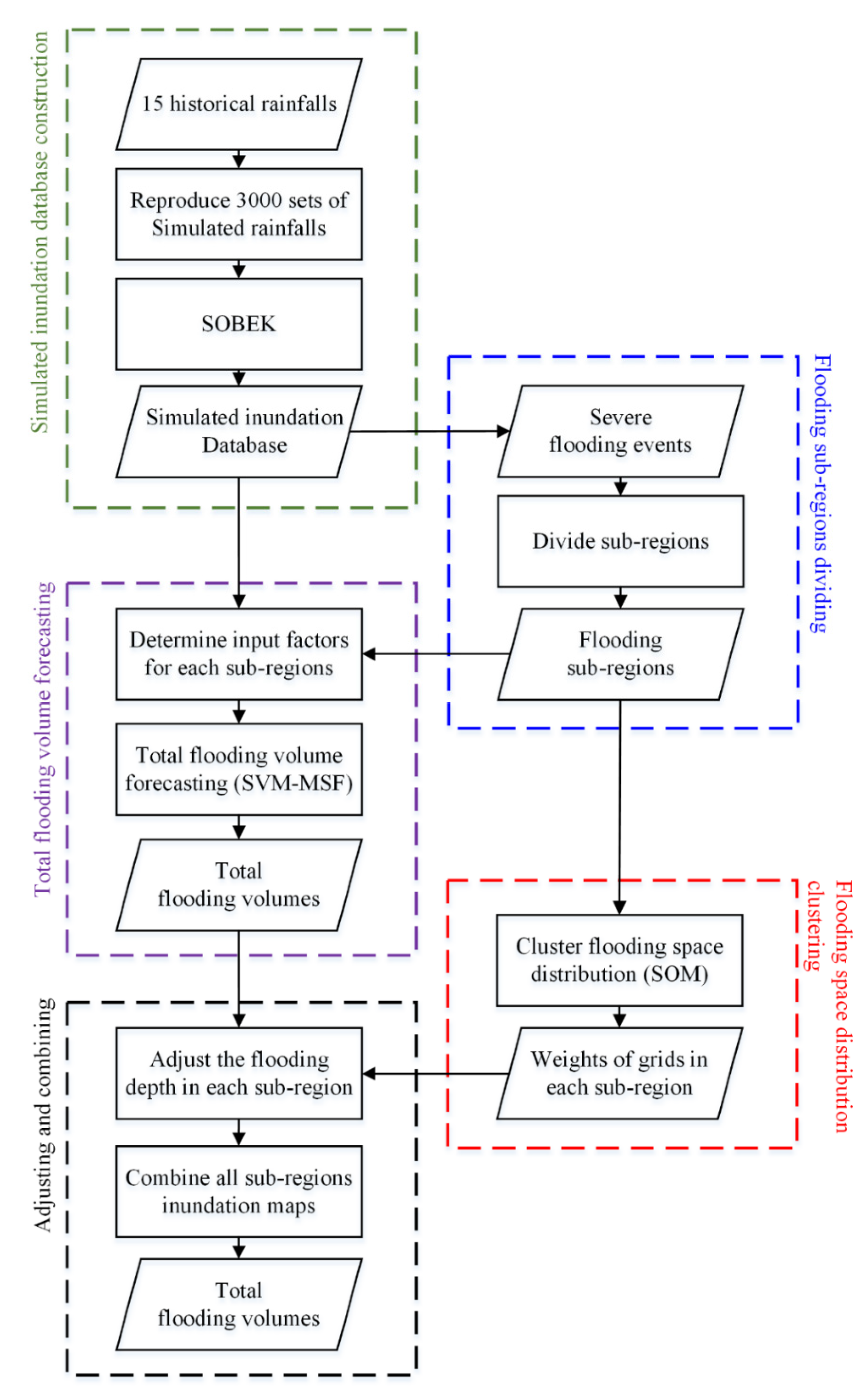
The results of the five steps mentioned in Section 3.1 are presented in this section. In Section 4.1, the flooding and virtual rainfall station sub-regions, which were divided by previous simulated flooding events, are shown. In Section 4.2, the results of the total flooding volume forecasted by SVM-MSF are illustrated. How SOM was used to classify the 3000 simulated flooding events into several categories results are shown in Section 4.3. Finally, the SVM-MSF and SOM merger results are presented in Section 4.4.

4.1. Sub-Region and Virtual Rainfall Station

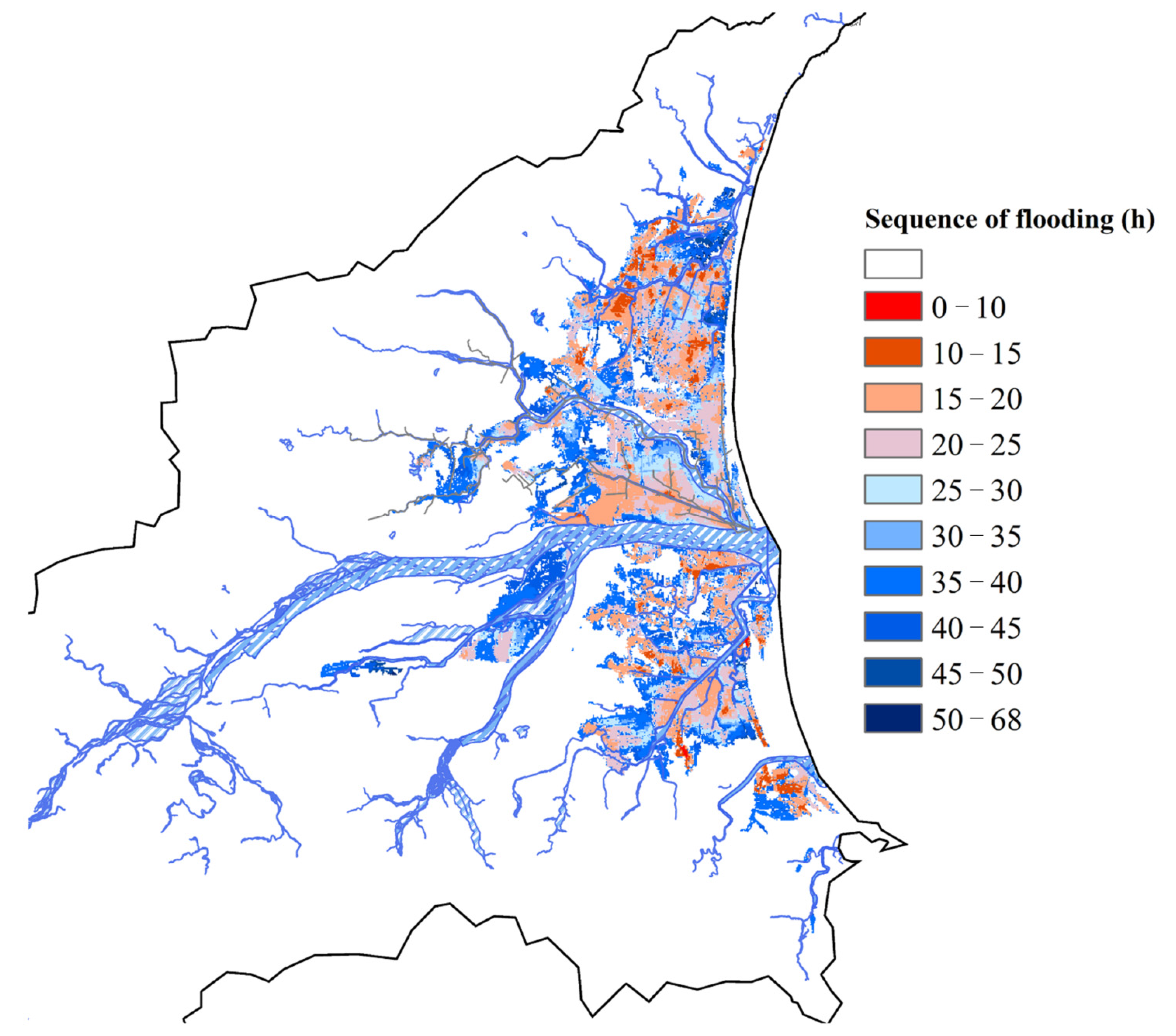
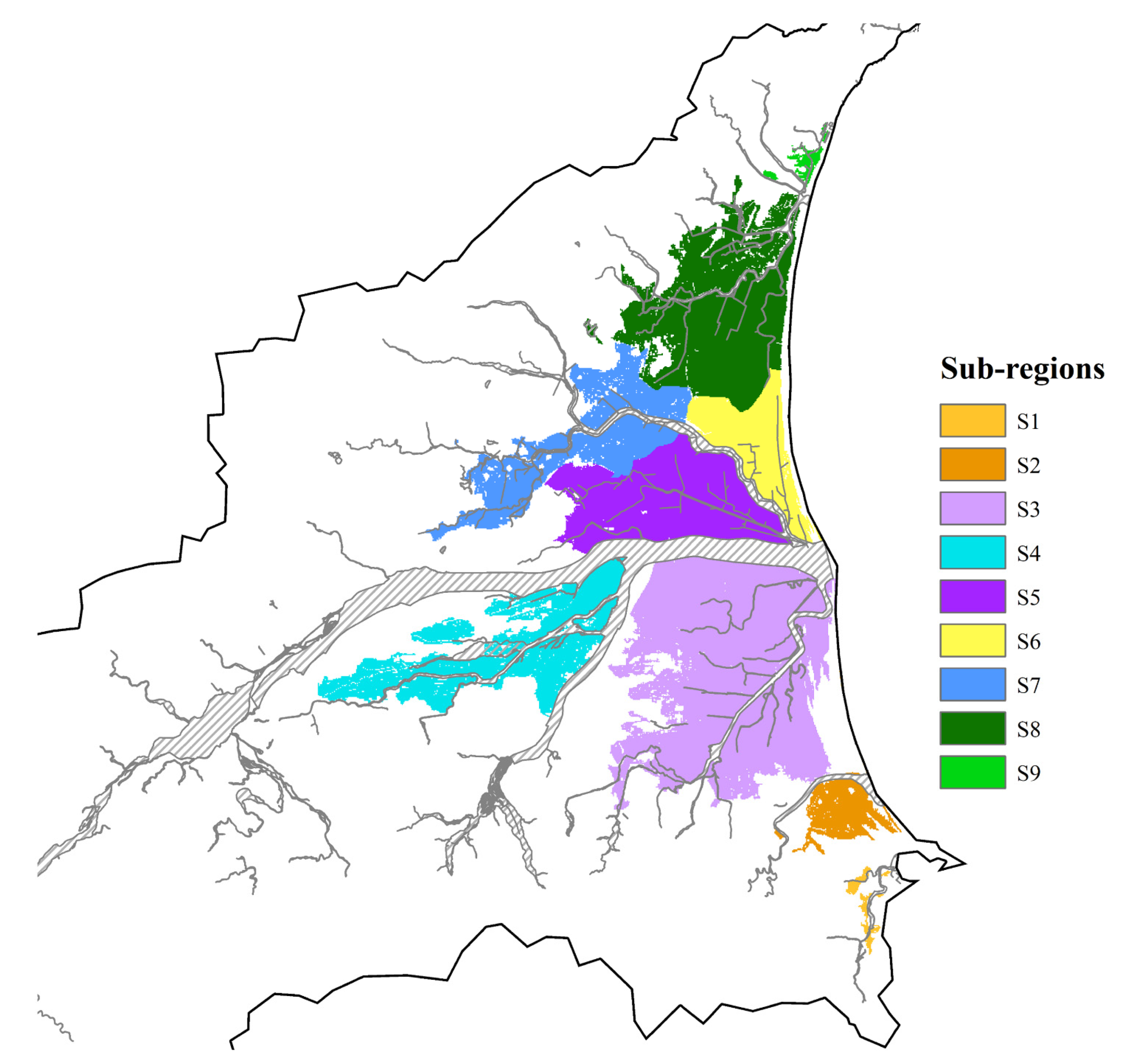
The most severe flooding event among the 3000 simulated flooding events was selected as the standard for dividing the flooding sub-regions in order to contain severe flooding characteristics. Figure 4 shows the order of the flood sequence; the colored labels in the figure represent the time when the grid began to flood. The grids closer to the dark red indicate earlier flooding and are regarded as the starting position for the flooding. Otherwise, the areas closer to the blue indicate the later flooding region. The interconnected red areas will be considered as the same starting position. By examining flooding sequences and watershed features, we judged which areas had the same flooding characteristics and divided them into nine sub-regions, as Figure 5 shows. From south to north, we named these sub-regions S1 to S9, respectively.

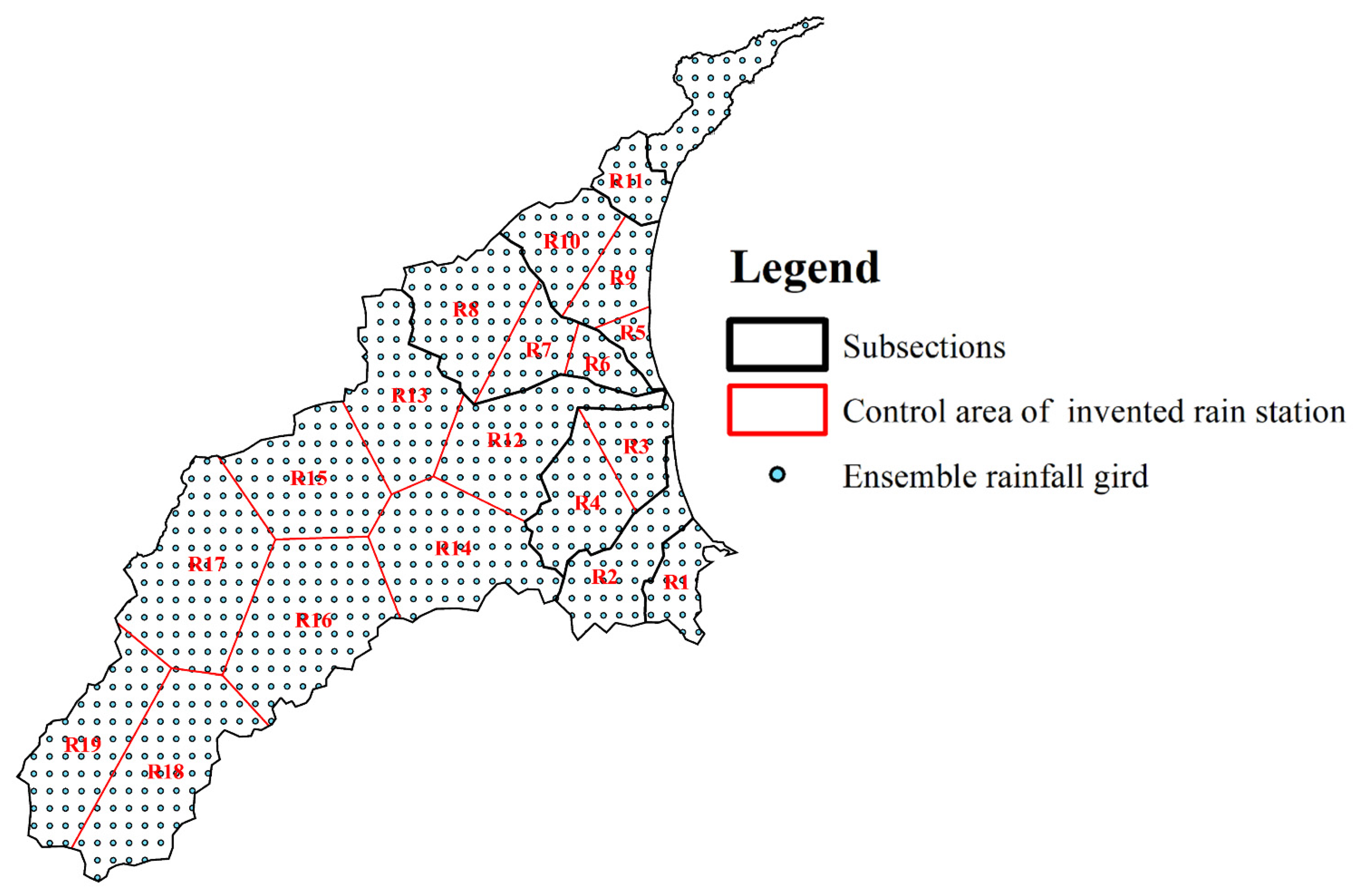
The ensemble gridded rainfall data used to construct the total flooding volume forecasting models in this study and the control area of each rainfall station are shown in Figure 6. Each spot on the figure represents the cumulative rainfall for an hour on the $20\times 20{ \mathrm{m}}^2$ grid. However, even though we had such detailed rainfall information, there were still two predicaments to be overcome. Too many adjacent rainfall inputs caused a high dependency and led the model to overfit. In addition, the huge number of inputs might lead to determination difficulties and long computational times, which cannot be applied in real time. For the above reasons, we simplified the rainfall inputs from original grids scaling to 19 virtual rainfall station data according to the catchments, control areas, and Thiessens’s polygon method. Given that mountainous rainfall cannot cause an immediate threat to urban flooding, a virtual rainfall station located in a mountainous area could cover a larger control area, such as virtual rainfall stations 15 to 19 on the left-hand side of the figure. On the contrary, the heavy rainfall in the urban area might lead to flood inundation caused by inner water rapidly rising. Hence, the control area of the virtual rainfall station, which was located in the metropolis, was smaller than those in the mountainous area.

4.2. Performance of SVM

As mentioned in Section 3.2, different parameter combinations for SVM would greatly affect model performance. The optimal parameters (kernel function, cost, ε, and γ) and input combinations determined by the grid search method are listed in

Table 2. The optimal parameters of SVM-MSF in nine sub-regions.

Sub-Region	Input	Kernel Function	Cost	ε	γ
S1	R1(t), R2(t)	RBF	2−1	2−7	2−3
S2	R1(t), R1(t − 1), R1(t − 2), R2(t), R2(t − 1), R2(t − 2)	RBF	23	2−7	2−3
S3	R3(t), R3(t − 1), R3(t − 2), R4(t)	RBF	2−3	2−7	23
S4	R12(t), R12(t − 1), R13(t), R13(t − 1), R13(t − 2), R14(t), R14(t − 1), R14(t − 2)	RBF	21	2−7	21
S5	R6(t), R6(t − 1), R6(t − 2)	RBF	2−3	2−7	2−3
S6	R5(t), R6(t), R6(t − 1), R6(t − 2), R7(t), R7(t − 1), R7(t − 2), R7(t − 3)	RBF	21	2−7	21
S7	R6(t), R7(t), R8(t), R8(t − 1), R8(t − 2)	RBF	21	2−7	23
S8	R9(t), R9(t − 1), R10(t), R10(t − 1), R10(t − 2)	RBF	2−1	2−7	23
S9	R11(t)	RBF	23	2−7	2−1

. We could summarize from the table that rainfall information upstream would take longer than rainfall information downstream. This pattern can be found most clearly in S6. For the downstream data (R5), there is only one hour of data required, and as the data areas move upstream, two hours (R6) and three hours (R7) of data are required. The pattern was in line with our assumptions on time of flow concentration that the early rainfall in mountainous areas would cause urban external water flooding. On the other hand, urban rainfall might directly cause accumulated flooding, so only short-term rainfall information was required. It is worth noting that rainfall data in mountainous areas (R15–R19) were not needed by the model for flood forecasting in urban areas. The determined results showed that rainfall in the mountainous areas of the study did not significantly flood the urban area, and the water source was mainly handled by the existing drainage system. For heavy rainfall events, urban floods were still dominated by local rainfall and near-regional rainfall.

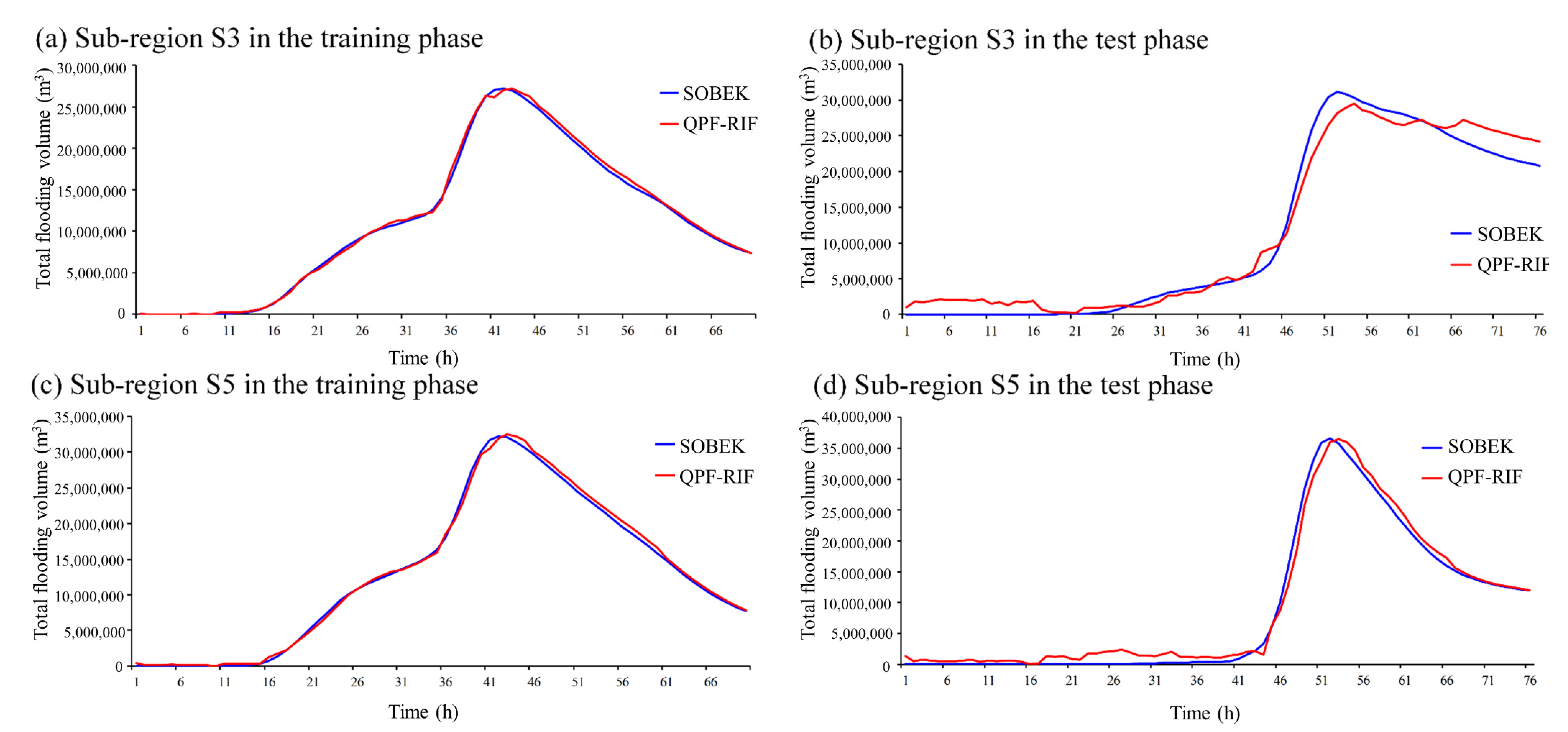
Due to the limited contexts, the performances of the model were presented with the most severe flooding events in training and testing events. That is, the following discussions focus on sub-region S3 (Donshan river) which had the maximum area, and sub-region S5 (Meifu drainage) which was the most prone to flooding and tended to flood most severely. The total flooding volume hydrographs were presented under two different conditions, short-term (t + 1) and long-term (t + 72) forecasting results. The results of the short-term forecast are shown in Figure 7. Figure 7a,c present the 1 h ahead forecasting results with the most severe flooding event in the training stage in the S3 and S5 sub-regions. The red curve represents the forecasting total flooding volume from the SVM-MSF model, and the blue curve was simulated by SOBEK. Each point of data in the red curve is the flooded volume predicted by the SVM-MSF using the input data available one hour before. As the figure shows, the results forecasted by SVM-MSF almost ideally fitted the SOBEK results, which were considered target values no matter the rising limb, falling limb, and even peak value. For the peak value timing forecasting, the lag time of the peak value was less than 0.5 h in the training phase. That is, there was no hysteresis effect when showing the training phase. In addition, according to the distance between the red and blue lines, the forecasting performance of sub-region S5 was slightly worse than that of S3. Nonetheless, the SVM-MSF forecasts are fairly close to the flooding simulations by SOBEK. The forecasting results in the testing phase, as Figure 7b,d shows, were slightly overestimated in the foremost flat period and falling limbs. For the rising limbs, it was slightly underestimated. These over- and underestimates were mainly caused by slight hysteresis forecasts, with the curve moving overall to the right. The lag time was also a trifle longer than the results in the training phases but could still last than an hour for the peak value forecasting. In sub-region S3, the model tended to underestimate the peak value. On the contrary, it accurately forecasted the peak value in sub-region S5 in spite of being overestimated in other segments. It was speculated that sub-region S3 faced more uncertainty due to the larger control area, which led to worse performance on peak value forecasting.

The performance measures of all sub-regions are listed in

Table 3. RMSE, MAE, CC, and CE of SVM-MSF in training and testing sections.

Sub-Region	RMSE (m)	MAE (m)	CC	CE
Training
1	6.65	5.38	0.70	0.81
2	5.10	3.56	0.99	0.82
3	6.12	4.52	0.99	0.98
4	1.20	0.76	0.90	0.90
5	16.75	12.03	0.98	0.90
6	7.72	6.03	0.99	0.96
7	3.33	2.62	0.91	0.91
8	6.41	5.12	0.99	0.99
9	2.83	2.15	0.98	0.98
Testing
1	6.02	5.21	0.67	0.82
2	4.86	3.48	0.99	0.98
3	5.82	4.45	0.99	0.98
4	1.16	0.74	0.90	0.92
5	16.13	11.73	0.99	0.95
6	7.52	5.86	0.99	0.98
7	3.31	2.60	0.94	0.92
8	6.20	4.99	0.99	0.99
9	2.61	2.01	0.98	0.96

. The RMSE and MAE listed in the table have been averaged by the gridded number of each sub-region and presented the mean of all grids. We derived from the performance measures that the RMSEs were less than 7.72 m³ and the MAEs were less than 6.03 m³ in all sub-regions except S5. Namely, the error of peak value and average flooding depth forecasting were both less than 5 mm. Even though the RMSE and MAE in sub-region S5 were higher than in other sub-regions, the average error of forecasting flood depth was still less than 1 cm. The rationale that the error of forecasting the flooding depth in sub-region S5 was higher than in the other sub-regions was that the uncertainty and scope of S5 were larger than the remaining eight sub-regions. In terms of CC, except for sub-region S1, the other eight sub-regions achieved excellent performance with a CC value higher than 0.9, no matter the training or testing scenarios. The CC value of sub-region S1 was 0.7. The reason that S1 had a worse performance was that fewer flooding events could be referred to, and the circumstances of each flood that could have occurred in S1 were very different, further increasing the difficulty of forecasting.

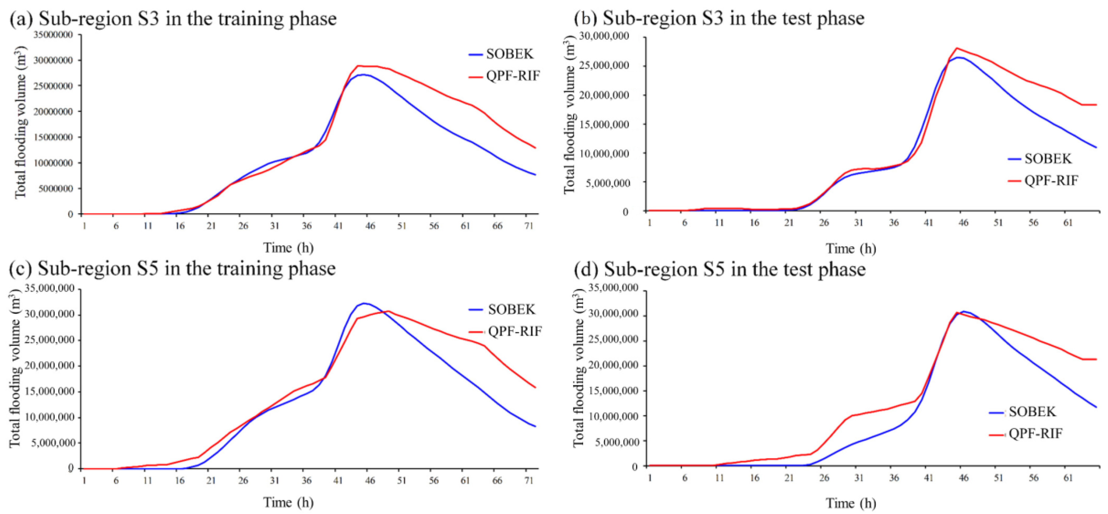
Figure 8 shows the long-term forecasting flooding volume hydrographs. The MSF results from forecasting 1 to 72 h ahead (t + 1 to t + 72) were shown in these figures. We also chose sub-regions S3 and S5 as representative analyses due to the space limitation. In sub-region S3, the SVM-MSF can accurately forecast the rising limbs and the timing of flooding peak (about 46 h lead time) both in the training and testing phases. Regarding the peak value and value of falling limbs, the model tended to slightly overestimate. On the other hand, in sub-region S5, no matter what phases tended to overestimate rising limbs and falling limbs. However, for peak value forecasting, the model effectively forecasted timing and value. It is worth noting that in the two sub-regions, there was no serious lag time hysteresis in the training or testing phases, mainly because our rainfall data contained more upstream rainfall data, which can contain future information. The existing lag time may come from the uncertainty of future on-site rainfall.

In summary, the SVM-MSF caught the trend of the total flooding volume no matter short-, mid-, or long-term forecasting, especially for characteristics of the peak value. The possible sources for errors in mid- and long-term forecasting were mainly the accumulative errors generated by recursive forecasting and the uncertainties from the numerical weather prediction system.

4.3. Performance of SOM

In this section, we are going to discuss the parameters used by the SOM and the topologies clustered by the SOM. First of all, the optimal parameters (determined by the grid search method) used in the SOM to classify several different types of inundation distribution are listed. In addition, the classified results are presented as average flooding depth maps. As in the previous sections, due to the space limitation of the article, in this section, we used sub-region S3 to discuss the determination process and the final training results of topology.

According to the principle of SOM, a reasonable topology size would highly affect the representativeness of the groups. Thus, we focused on the determination of topology size in this section.

Table 4. Determination of SOM in sub-region S3.

Topo Size	RMSE (m)	MAE (m)
5 × 5	0.079	0.034
6 × 6	0.084	0.033
7 × 7	0.091	0.039
8 × 8	0.093	0.039
9 × 9	0.083	0.034

shows the classified results in sub-region S3 with different topology sizes. To quantify the model performance, RMSE and MAE were also employed as a benchmark for the forecasting error of the maximum flooding and average depths. As the table shows, the model had the best RMSE and second place MAE, while the topology size was settled as $5\times 5$. When using the topology size $5\times 5$, the RMSE improved by 5% compared with the suboptimal solution of $9\times 9$, while the MAE part only increased by 3% compared with the suboptimal solution of $6\times 6$. Given that disaster researchers often concentrate more on situations with severe disasters, RMSE optimized by 5% should be considered a critical factor. In view of this, the optimal topology size for sub-region S3 was $5\times 5$. Other sub-regions were determined by the topology size with the same standards. The other optimal sizes of topologies are listed in

Table 5. The optimal parameters of SOM.

Sub-Region	Topo Size	RMSE (m)	MAE (m)
S1	9 × 9	0.0135	0.0009
S2	8 × 8	0.0458	0.0034
S3	5 × 5	0.0790	0.0099
S4	9 × 9	0.0242	0.0011
S5	7 × 7	0.1199	0.0264
S6	9 × 9	0.0411	0.0035
S7	9 × 9	0.0721	0.0086
S8	7 × 7	0.0890	0.0165
S9	5 × 5	0.0367	0.0029

. As shown in the table, the RMSEs and MAEs of sub-regions S3, S5, and S8 were higher than those of the others. The reason was that these three sub-regions were the areas with the most severe flooding conditions (located downstream of major rivers), which was consistent with the actual situation of flooding.

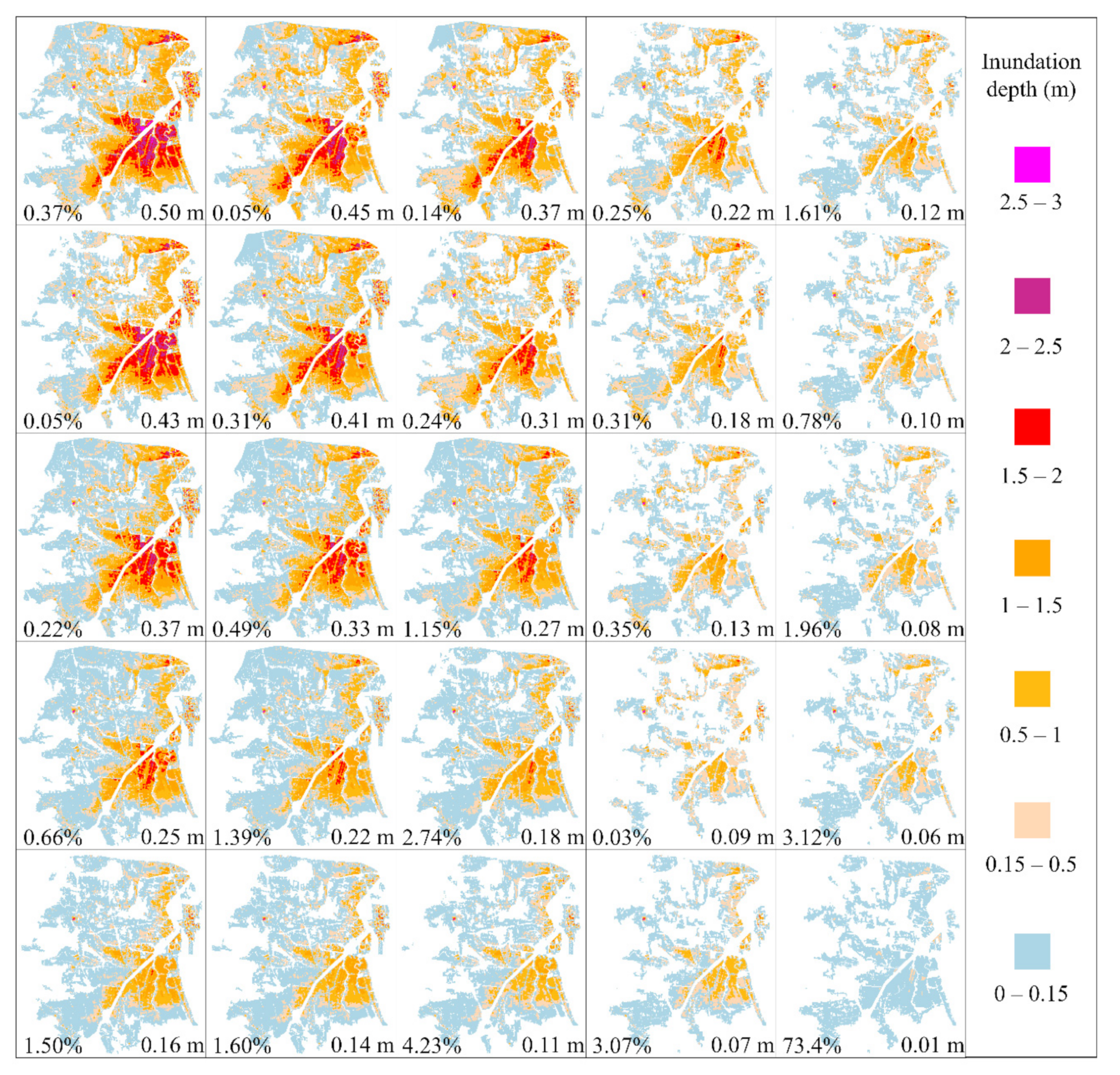
According to the determination previously mentioned, 3000 sets of simulated flooding events in sub-region S3 were divided into 25 categories with SOM. The clustering results by SOM, without artificial ranking, are shown in Figure 9. The values in the lower left corner of sub-figures indicate the proportion of this category in all training data, and the lower right corner shows the average flooding depth of all the grids in each category. With these values, we analyzed the probability of floods in this category and how severe the flooding was. As shown in the lower-left corner of the graph, although in the flooding database, there were still 73.4% flooding maps, the average flooding depth was less than 1 cm. As the average flooding depth of the grid increased, the probability of its occurrence significantly decreased. However, when the average depth of flooding was higher than 0.1 m, the odds for all groups were fairly close. This phenomenon reflected the climate characteristics in the study area. When moderate rainfall or long-term weak rainfall occurred, there were very few floods in the area, and most floods were caused by extreme weather events. From flood depth and distribution analysis, each adjacent flooding map had high correlations, and the average flood depth gradually increased from the bottom right category to the top left category. To be more specific, each category had its own unique characteristics; from the right category to the left, it was found that the categories tended to gradually increase the flooding range. On the other hand, from the bottom category to the top, it tended to deepen the flooded area.

4.4. Adjusted and Combined Results

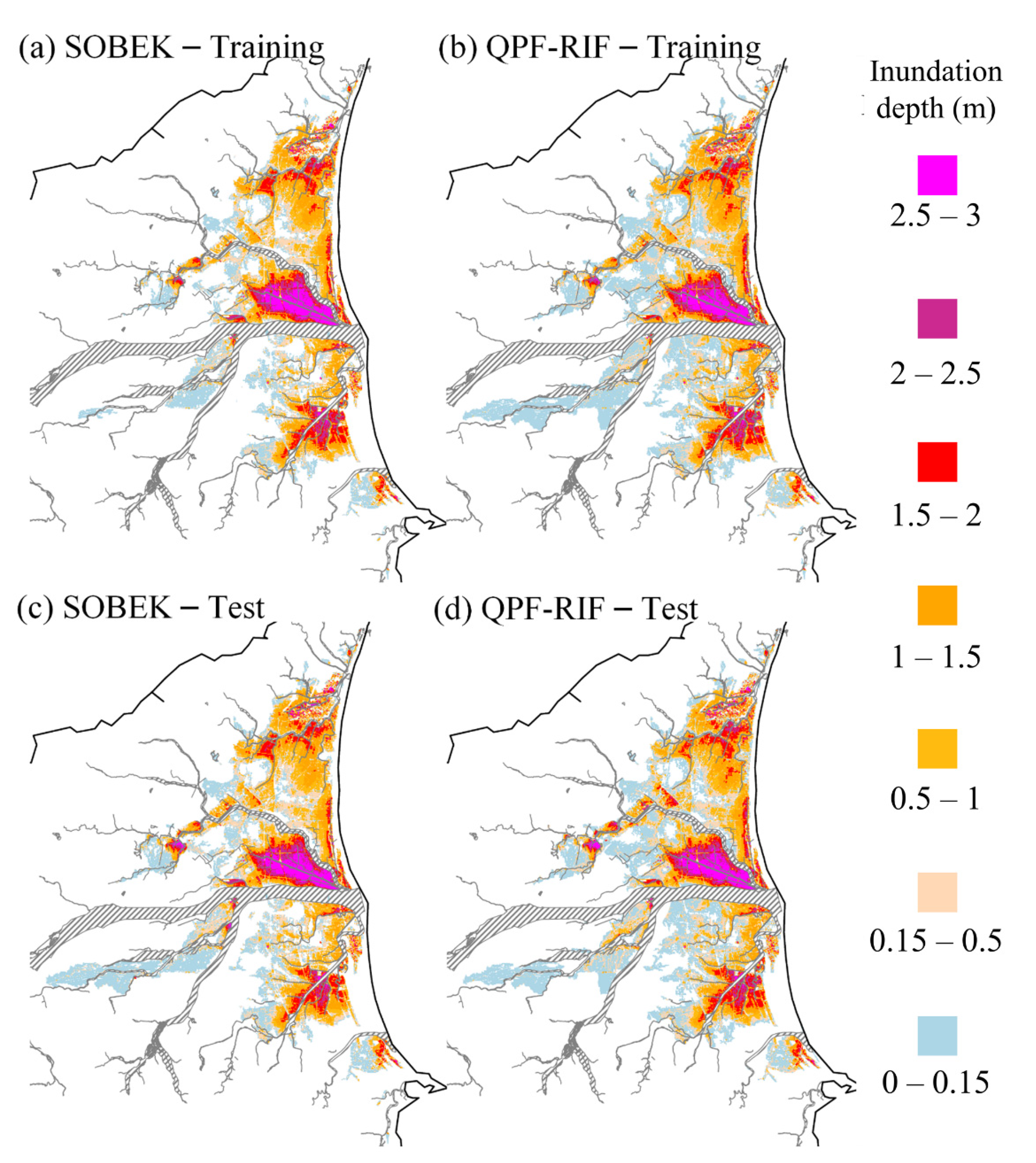
The Yilan County-wide flooding depth forecasting maps were generated by combining the results of SVM-MSF and SOM clustering and were named QPF-RIF. For the demonstration event, the most severe training and testing events in the database were selected, and the timing was the time when the flooding depth was the deepest (approximately 51 h). The results of flooding depth forecasting maps are shown in Figure 10. On the left-hand side, Figure 10a shows the flooding depth map simulated by SOBEK, Figure 10b is the forecasting result from QPF-RIF in the most severe training event, and Figure 10c,d is from the testing event. As mentioned in the previous section, the most severely flooded sub-regions during historical events were S3, S5, and S8, which is in line with the situation in this event. As the figure shows, the flooding depth map can accurately be forecasted by the QPF-RIF proposed in this study. A flooding area shallower than 0.15 m is shown as light blue in this figure. The range of the inundation zone exceeding 0.15 to 3 m is marked in sequence from light blue to purple, as the labels show. From Figure 10, regardless of the events of the training or testing groups, the results of the SOBEK simulated severe flooding area (deeper than 0.15 m) are quite close to that of the long-term QPF-RIF forecasts, both in terms of inundation range and depth indication. The obvious disadvantage of QPF-RIF was that the forecast in the light blue area was larger than that simulated by the SOBEK model. The main reason was that the group average mentioned in Section 4.3 contained information from multiple events. The shallow flooding areas may have occurred at some points in the remaining events, which were taken into account by the model. Although shallow flooding areas may be overestimated, it is enough to confirm that QPF-RIF proposed in this study is able to effectively simulate the flooding depths close to those resulting from SOBEK, which are considered actual values in this study.

Besides the simulated events, the model was also calibrated by recent heavy rainfall and typhoon events. There must be sufficient rainfall intensity and flooding-related data collected for the selected events. Thus, during the heavy rainfall event on 11 October 2017, Typhoons Saola, Megi, and Migta were adopted.

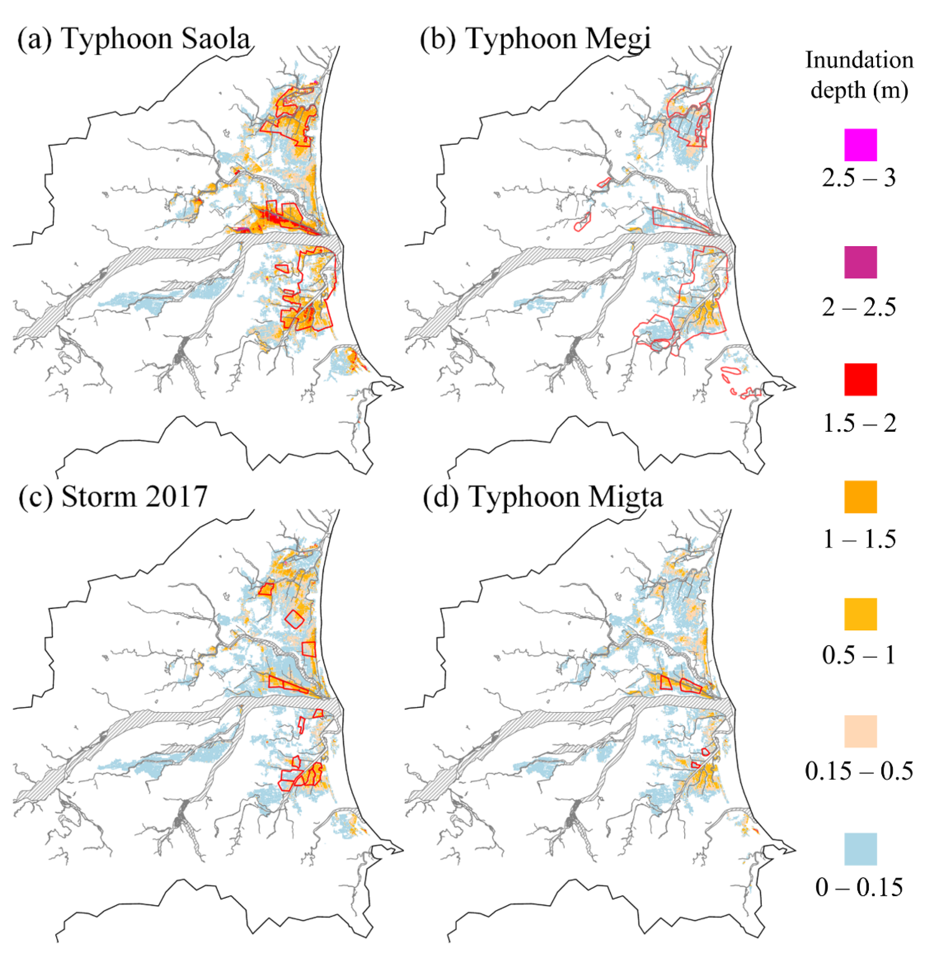
Figure 11 shows the comparisons between the flooding depth forecasted by QPF-RIF and the EMIC report information mentioned in Section 2. In Figure 11a, the forecasted flooding depth and EMIC of Typhoon Saola are shown. The color of each grid represents the depth of flooding forecasted by QPF-RIF, and the area marked by the red line is the actual flooding area framed according to the EMIC. Compared with EMIC data, in the S3, S5, and S8 sub-regions, models accurately forecasted the flooding area, especially in areas with severe inundation (both sides of the riverbanks and low-lying urban areas). As forecasts from the model, the local flooding depth in these three areas was deeper than 0.5 m, which was also close to the actual flooding depth of the most serious flooding position in the reported data.

The forecasting result of Typhoon Megi is plotted in Figure 11b. As shown in the figure, the floods in this event were milder than those in Typhoon Saola, and the flooding areas of Typhoon Megi were more dispersed, such as in sub-region S1 and the upper reaches of the Yilan River. In general, except for some underestimations downstream of sub-regions S3 and S8, other flooding areas and levels were effectively forecasted. Figure 11c shows the comparison between the flooding depth forecasted by the QPF-RIF and the EMIC using the heavy rainfall event data on 11 October 2017. According to the EMIC report, flooding occurred in sub-region S3 with a depth ranging from 0 to 90 cm. The model forecasted flooding area was indeed highly similar to the grids from EMIC. The partial grids forecasted flooding depths greater than 15 cm and, even rarer, deeper than 1 m, which was similar to the reported information. There were also some small flooding areas reported in sub-regions S6, S9, and the right bank of S5. The depths forecasted in these areas were also similar to the EMIC data. In general, most areas with severe flooding can be pre-warned by QPF-RIF forecasting in this heavy rainfall case. Finally, the comparison between the forecasted results and the range of EMIC in Typhoon Migta is shown in Figure 11d. According to the EMIC report, flooding that occurred in sub-regions S3 and S5 was lesser than that in Typhoon Megi. Only small-scale shallow water was reported in sub-region S3. In the sub-region S5, the flooding depth of the EMIC report was about 0.5 to 1 m, which was similar to the forecasting value.

The EMIC-reported information did not perfectly represent all the flooded locations in the study area during the historical events and was based on the results of surveys from residents and public officials. The full confusion matrix cannot be used in this study due to data limitations. Hence, in the following, the TPR (used in the confusion matrix) will be adopted to calculate the forecast accuracy in the EMIC flooding range to quantify the model performance. The TPRs of five historical storm events are listed below in

Table 6. TPR of adjusted and combined results with different flooding standards.

Event	TPR (%)
	Threshold 0 *	Threshold 0.15 *	Threshold 0.30 *
Parma	64	26	17
Megi	54	20	12
Saola	83	63	54
Storm 2017	77	63	26
Migta	89	61	49

* Thresholds 0, 0.15, and 0.30 represent that only the water depth over 0, 0.15, and 0.3 m were considered as inundation.

under three different flooding standards (0, 0.15, and 0.30 m). Standard 0 represents the area where the water level was over 0 cm, as seen as a flooding area, the standard 15 and standard 30 represent the same. As Table 6 shows, QPF-RIF forecasted about 83% of the flooding area of the EMIC reports in Typhoons Saola, Migta, and the storm in 2017 under standard 0. That is, the model forecasted over 80% of the inundation area no matter how shallow the water or severe the inundation. Limited by the contents of EMIC reports, the information cannot correctly reflect the real depth of floods. However, we still can use standards 15 and 30 to evaluate the proportion of the area suffering from the disaster in this event. As standard 15 shows, in the last three events, the ratio of the flooding area over 15 cm to the total EMIC-reported area was about 60%. For standard 30, the proportions of each event were quite different. In Typhoons Saola and Migta, the area that flooded deeper than 30 cm was over half of the total EMIC-reported area. On the other hand, in other events, the flooding area over 30 cm was less than 30%. We can use these thresholds to determine whether the flooding in this rainfall event was a shallow and harmless event or a situation that will actually cause economic losses.

In addition, the TPRs in Typhoons Parma and Megi were obviously smaller than the other three events. The rationale was that large-scale hydraulic structures were built in the study area in 2012, which led to quite different flooding characteristics after 2012. As mentioned in Section 2, the study area and data used to construct the SOBEK model were updated in 2019. Thus, the model was reasonable to underestimate the inundation severity for typhoon events that happened before 2012. The TPRs of standard 0 showed the accuracy of events after 2012 at an average of 24% higher than those before 2012. Also, the TPRs of standards 15 and 30 have substantial differences. The proof model does have the ability to catch flood protection by hydraulic structures.

In sum, the results of this research proved that QPF-RIF has sufficient ability to forecast the medium- and long-term flooding range and depth, especially in severely flooded areas. It can effectively assist in policy formulation, pump scheduling, and disaster prevention operations.

5. Conclusions

In this study, we proposed QPF-RIF, which can forecast the future (72 h lead time) flooding depth maps without setting up urban flood monitoring stations and was constructed by the simulated flooding database.

The results can be consolidated into the following points. Firstly, the 1 h ahead forecasting results of SVM-MSF can almost perfectly fit the total flooding volume simulated by SOBEK, and the average error of flooding depth can be controlled by less than 1 cm. It can effectively provide, more than 46 h ahead, advance forecasts under the condition that the forecasting ensemble rainfall data is credible. Secondly, we could obviously discover that the clustering algorithm used in this study can effectively distinguish severe flooding in various types of flooding areas or large-scale shallow areas. Also, it can accurately map the total flooding volume to each grid, and the average error of all the grids is within 7 cm. Thirdly, the flooding depth maps forecasted by QPF-RIF, which was fused by SVM-MSF and SOM, could be highly analogous to the maps simulated by SOBEK seen as the target value in this study, especially for areas with severe flooding and has a more accurate performance. There might be slight overestimations for slight water accumulative grids, and this does not affect the accuracy of the overall availability. Finally, verification results for three typhoons and one single heavy rainfall event demonstrate that the QPF-RIF has highly flooding depth and range forecasting capabilities (83% of flooding area). Except for a few areas where flooding has not been simulated in the flooding database and cannot be accurately forecasted, QPF-RIF can effectively and accurately forecast flood-prone areas and deeper flooding areas several hours ahead.

In conclusion, the QPF-RIF proposed in this study can accurately forecast the long-term flooding distribution and depth and provide more reliable real-time and future information. In the future, reducing the uncertainty caused by the forecasting ensemble rainfall data and incorporating real-time monitoring data, such as applying machine learning methods, statistical methods, and mobile pumping station information to achieve the purpose of real-time correction of the inundation maps, might be feasibility challenged.

References

1. Beven, K.J.; Kirkby, M.J.; Schofield, N.; Tagg, A.F. Testing a physically-based flood forecasting model (TOPMODEL) for three UK catchments. J. Hydrol. 1984, 69, 119–143. [Google Scholar] [CrossRef]
2. Ji, Z.; De Vriend, H.; Hu, C. Application of SOBEK model in the Yellow River estuary. In Proceedings of the International Conference on Estuaries and Coasts, Hangzhou, China, 9–11 November 2003; Available online: http://www.irtces.org/pdf-hekou/114.pdf (accessed on 28 August 2022).
3. Santhi, C.; Arnold, J.G.; Williams, J.R.; Dugas, W.A.; Srinivasan, R.; Hauck, L.M. Validation of the swat model on a large rwer basin with point and nonpoint sources. J. Am. Water Resour. Assoc. 2001, 37, 1169–1188. [Google Scholar] [CrossRef]
4. Betrie, G.D.; van Griensven, A.; Mohamed, Y.A.; Popescu, I.; Mynett, A.E.; Hummel, S. Linking SWAT and SOBEK using open modeling interface (OPENMI) for sediment transport simulation in the Blue Nile River basin. Trans. ASABE 2011, 54, 1749–1757. [Google Scholar] [CrossRef]
5. Han, D.; Chan, L.; Zhu, N. Flood forecasting using support vector machines. J. Hydroinf. 2007, 9, 267–276. [Google Scholar] [CrossRef]
6. Chang, L.C.; Shen, H.Y.; Wang, Y.F.; Huang, J.Y.; Lin, Y.T. Clustering-based hybrid inundation model for forecasting flood inundation depths. J. Hydrol. 2010, 385, 257–268. [Google Scholar] [CrossRef]
7. Pyayt, A.L.; Mokhov, I.I.; Lang, B.; Krzhizhanovskaya, V.V.; Meijer, R.J. Machine learning methods for environmental monitoring and flood protection. World Acad. Sci. Eng. Technol. 2011, 78, 118–123. [Google Scholar]
8. Aggarwal, S.K.; Goel, A.; Singh, V.P. Stage and discharge forecasting by SVM and ANN techniques. Water Resour. Manag. 2012, 26, 3705–3724. [Google Scholar] [CrossRef]
9. Vadiati, M.; Rajabi Yami, Z.; Eskandari, E.; Nakhaei, M.; Kisi, O. Application of artificial intelligence models for prediction of groundwater level fluctuations: Case study (Tehran-Karaj alluvial aquifer). Environ. Monit. Assess. 2022, 194, 619. [Google Scholar] [CrossRef]
10. Samani, S.; Vadiati, M.; Azizi, F.; Zamani, E.; Kisi, O. Groundwater Level Simulation Using Soft Computing Methods with Emphasis on Major Meteorological Components. Water Resour. Manag. 2022, 36, 3627–3647. [Google Scholar] [CrossRef]
11. Li, T.; Lu, J.; Wu, J.; Zhang, Z.; Chen, L. Predicting Aquaculture Water Quality Using Machine Learning Approaches. Water 2022, 14, 2836. [Google Scholar] [CrossRef]
12. Derdour, A.; Jodar-Abellan, A.; Pardo, M.Á.; Ghoneim, S.S.M.; Hussein, E.E. Designing Efficient and Sustainable Predictions of Water Quality Indexes at the Regional Scale Using Machine Learning Algorithms. Water 2022, 14, 2801. [Google Scholar] [CrossRef]
13. Ha, M.C.; Vu, P.L.; Nguyen, H.D.; Hoang, T.P.; Dang, D.D.; Dinh, T.B.H.; Şerban, G.; Rus, I.; Brețcan, P. Machine Learning and Remote Sensing Application for Extreme Climate Evaluation: Example of Flood Susceptibility in the Hue Province, Central Vietnam Region. Water 2022, 14, 1617. [Google Scholar] [CrossRef]
14. Tanim, A.H.; McRae, C.B.; Tavakol-Davani, H.; Goharian, E. Flood Detection in Urban Areas Using Satellite Imagery and Machine Learning. Water 2022, 14, 1140. [Google Scholar] [CrossRef]
15. Farhadi, H.; Esmaeily, A.; Najafzadeh, M. Flood monitoring by integration of Remote Sensing technique and Multi-Criteria Decision Making method. Comput. Geosci. 2022, 160, 105045. [Google Scholar] [CrossRef]
16. Farhadi, H.; Najafzadeh, M. Flood Risk Mapping by Remote Sensing Data and Random Forest Technique. Water 2021, 13, 3115. [Google Scholar] [CrossRef]
17. Chang, H.K.; Lin, Y.J.; Lai, J.S. Methodology to set trigger levels in an urban drainage flood warning system–an application to Jhonghe, Taiwan. Hydrol. Sci. J. 2017, 63, 31–49. [Google Scholar] [CrossRef]
18. Chang, M.J.; Chang, H.K.; Chen, Y.C.; Lin, G.F.; Chen, P.A.; Lai, J.S.; Tan, Y.C. A support vector machine forecasting model for typhoon flood inundation mapping and early flood warning systems. Water 2018, 10, 1734. [Google Scholar] [CrossRef] [Green Version]
19. Chang, T.J.; Wang, C.H.; Chen, A.S. A novel approach to model dynamic flow interactions between storm sewer system and overland surface for different land covers in urban areas. J. Hydrol. 2015, 524, 662–679. [Google Scholar] [CrossRef] [Green Version]
20. Chang, L.C.; Chang, F.J.; Wang, Y.P. Auto-configuring radial basis function networks for chaotic time series and flood forecasting. Hydrol. Process. 2009, 23, 2450–2459. [Google Scholar] [CrossRef]
21. Chang, L.C.; Shen, H.Y.; Chang, F.J. Regional flood inundation nowcast using hybrid SOM and dynamic neural networks. J. Hydrol. 2014, 519, 476–489. [Google Scholar] [CrossRef]
22. Wu, R.-S.; Sin, Y.-Y.; Wang, J.-X.; Lin, Y.-W.; Wu, H.-C.; Sukmara, R.B.; Indawati, L.; Hussain, F. Real-Time Flood Warning System Application. Water 2022, 14, 1866. [Google Scholar] [CrossRef]
23. Wu, S.-J.; Hsu, C.-T.; Shen, J.-C.; Chang, C.-H. Modeling the 2D Inundation Simulation Based on the ANN-Derived Model with Real-Time Measurements at Roadside IoT Sensors. Water 2022, 14, 2189. [Google Scholar] [CrossRef]
24. Vapnik, V. The Nature of Statistical Learning Theory; Springer Science and Business Media: Berlin, Germany, 1995. [Google Scholar]
25. Vapnik, V. Statistical Learning Theory; Wiley: New York, NY, USA, 1998. [Google Scholar]
26. Kohonen, T. Self-organized formation of topologically correct feature maps. Biol. Cybern. 1982, 43, 59–69. [Google Scholar] [CrossRef]
27. Kohonen, T. The self-organizing map. Proc. IEEE 1990, 78, 1464–1480. [Google Scholar] [CrossRef]
Figure 1. Study area.
Water 14 03346 g001
Figure 2. Flowchart of research.
Water 14 03346 g002
Figure 3. The structures of (a) SVM and (b) SOM.
Water 14 03346 g003
Figure 4. The order in which flooding occurred.
Water 14 03346 g004
Figure 5. Nine sub-regions in Yilan County divided by flooding characteristics.
Water 14 03346 g005
Figure 6. The mesh of ensemble rainfall and virtual rainfall stations settle in this study.
Water 14 03346 g006
Figure 7. Comparison of the total flooding volume for 1 h lead-time forecasts of the SOBEK and SVM-MSF for S3 and S5 in the training and testing phases.
Water 14 03346 g007
Figure 8. Comparison of the total flooding volume from 1 to 72 h lead-time forecasts of the SOBEK and SVM-MSF for S3 and S5 in the training and testing phases.
Water 14 03346 g008
Figure 9. The results of SOM classification.
Water 14 03346 g009
Figure 10. Comparing the flooding maps simulated by SOBEK and forecasted by QPF-RIF in the training and testing phases.
Water 14 03346 g010
Figure 11. Comparing the flooding maps forecasted by QPF-RIF and flooding area reported by EMIC in 4 historical events.
Water 14 03346 g011