


Impacts of Spatial Interpolation Methods on Daily Streamflow Predictions with SWAT

Department of Civil Engineering, Chungnam National University, Daejeon 34134, Korea
*
Author to whom correspondence should be addressed.
Water 2022, 14(20), 3340; https://doi.org/10.3390/w14203340
Submission received: 17 August 2022
/
Revised: 15 October 2022
/
Accepted: 19 October 2022
/
Published: 21 October 2022
(This article belongs to the Special Issue SWAT Modeling - New Approaches and Perspective)
Abstract
:Precipitation is a significant input variable required in hydrological models such as the Soil & Water Assessment Tool (SWAT). The utilization of inaccurate precipitation data can result in the poor representation of the true hydrologic conditions of a catchment. SWAT utilizes the conventional nearest neighbor method in assigning weather parameters for each subbasin; a method inaccurate in representing spatial variations in precipitation over a large area, with sparse network of gauging stations. Therefore, this study aims to improve the spatial variation in precipitation data to improve daily streamflow simulation with SWAT, even pre-model calibration. The daily streamflow based on four interpolation methods, nearest neighbor (default), inverse-distance-weight, radial-basis function, and ordinary kriging, were evaluated to determine which interpolation method is best represents the precipitation at Yongdam watershed. Based on the results of this study, the application of spatial interpolation methods generally improved the performance of SWAT to simulate daily streamflow even pre-model calibration. In addition, no universal method can accurately represent the long-term spatial variation of precipitation at the Yongdam watershed. Instead, it was observed that the optimal selection of interpolation method at the Yongdam watershed is dependent on the long-term climatological conditions of the watershed. It was also observed that each interpolation method was optimal based on certain meteorological conditions at Yongdam watershed: nearest neighbor for cases when the occurrence probability of extreme precipitation is high during wet to moderately wet conditions; radial-basis function for cases when the number of dry days were high, during wet, severely dry, and extremely dry conditions; and ordinary kriging or inverse-weight-distance method for dry to moderately dry conditions. The methodology applied in this study improved the daily streamflow simulations at Yongdam watershed, even pre-model calibration of SWAT.
1. Introduction
Precipitation inputs are the main driving force of hydrological models [1,2]. Soil & Water Assessment Tool (SWAT) is a widely recognized hydrological model utilized to simulate long-term hydrologic outputs such as streamflow [1,2,3,4,5,6,7,8,9], and water quality [1,4] in gauged and ungauged catchments [10]. Alongside precipitation, SWAT requires five more weather inputs: minimum and maximum temperatures, humidity, solar radiation, and wind speed [10,11]. These weather parameters are recorded from ground observation stations usually installed in distant intervals. While data from ground observation stations can represent the meteorological conditions in its vicinity, it cannot represent the spatial variation of weather parameters over large areas, especially for sparse and heterogenous network of observation stations [1]. The inaccurate representation of these weather variables in hydrological models, especially precipitation, results in the poor representation of the natural hydrologic conditions of a watershed, such as streamflow and water quality. Thus, improving the spatial representation of precipitation inputs in hydrological models, such as SWAT, is necessary to accurately simulate model outputs such as streamflow.
To improve the spatial representation of precipitation inputs in SWAT, previous research has utilized the spatial interpolation methods on ground station data [1,2,3,4,6,7,8,9]. Subsequently, the aforementioned studies [1,2,3,4,6,7,8,9] validated the spatially interpolated precipitation datasets through the comparison between the observed and predicted datasets. Zeiger and Hubbart [3] also applied the same methodology and also proposed to use a pre-calibrated model when validating the spatial interpolation methods, to isolate the effects of the methods from other model parameters, when simulating streamflow.
The interpolation methods utilized from previous studies [1,2,3,4,6,7,8,9] are either classified as deterministic [1,2,3,4,6,7,8,9] or geostatistical [3,4,6,7,8] interpolation methods. Among the deterministic methods successfully applied were: Thiessen polygon [12] or nearest neighbor method (NN) [1,2,4,6,7], inverse-distance-weight (IDW) [1,2,4,6,7,9], and spline [3]; the geospatial methods applied were: co-kriging [7], kriging with external drift [4], ordinary kriging (OK) [3,4,6], and universal kriging [3]. While previous studies [1,2,3,4,6,7,8,9] proved the hypothesis that applying interpolation methods on daily precipitation in SWAT improves the overall performance of the model to simulate daily streamflow, the optimal method concluded from each study varied and did not reach a consensus due to the diversity in research methodology applied. For example, the threshold value to differentiate precipitation intensities, detailed information on the long-term meteorological conditions of the watershed, and various interpolation tools utilized (i.e., grid sizes, weights, and the number of neighboring stations considered during the interpolation process). Moreover, the difference in the results can also be attributed to various factors such as the: catchment size, climate zone conditions, integrity of climate data, the density of gauging stations, and the topographic characteristics of the study area. Without including these aforementioned details, the research results presented can only be interpreted as basin-specific findings. However, if those details were included for each study, generalized findings can be subsequently derived after several studies. While basin-specific findings are important, presenting generalized findings (e.g., optimal interpolation method based on the station density, or hydrological conditions of a basin) is equally significant to determine the general applicability of each interpolation method.
Among the current literature published related to the evaluation of spatial interpolation methods to improve streamflow predictions in SWAT [1,2,3,4,6,7,8,9], only Cheng et al. [7] presented quasi-generalized results, by determining the applicability of each interpolation method based on precipitation intensities. Cheng et al. [7] concluded that TP, IDW, and CK methods outperformed the default NN method for periods with heavy precipitation patterns (i.e., wet period), and NN performed best for light precipitation. While the methodology presented by Cheng et al. [7] is promising in terms of providing both basin-specific and quasi-general findings, further improvements in the methodology can be suggested as follows: (1) defining the exact threshold values to classify precipitation intensities based on known standard, in order to reach objective conclusions; (2) and by skipping the tedious process of using the GIS program to do the daily interpolations, through the use of a pre-processing program. Unfortunately, several researchers [1,2,3,6,8] went through the tedious process of using GIS software to apply spatial interpolation methods on precipitation inputs, before SWAT applications. Masih et al. [2] applied a single interpolation method on daily precipitation for 15 years and specified the potential convenience for SWAT users if an optional component can execute the interpolation of weather input data.
In this study, an improved methodology is proposed to resolve several research gaps in existing methodologies on the improvement of SWAT precipitation inputs in simulating daily streamflow at the Yongdam watershed. The detailed objectives of this study are summarized as follows: (1) to evaluate the applicability of the pre-processing tool to generate daily precipitation inputs, with better spatial variation, to improve daily streamflow simulation with SWAT; (2) to determine the applicability of each interpolation method based on different classifications of precipitation intensities (i.e., classified by the World Meteorological Organization [13]); and (3) to analyze the impacts of various spatial interpolation methods on daily streamflow predictions with SWAT even pre-model calibration (i.e., to isolate the effects of precipitation inputs from other model parameters [3]).
The structure of this paper is summarized as follows: Section 2 includes the description of models and spatial interpolation methods, and an introduction of the study area and input data utilized in this study; the results and discussions are presented in Section 3; and finally, the major findings and future research directions are summarized in Section 4.
2. Materials and Methods
2.1. SWAT
Soil and Water Assessment Tool (SWAT) is a semi-distributed, processes-based watershed model that operates on a daily time step, utilized to evaluate the effects of land use on streamflow, and sediment management in gauged, and ungauged catchments [10]. SWAT divides the watershed into multiple subbasins based on the user-defined stream network threshold value. The subbasins are further subdivided into smaller hydrologic response units (HRUs), which are composed of unique combinations of land use, soil characteristics, and slope to form a homogeneous unit.
Water balance is the driving mechanism responsible for all processes within the model, and causes direct effects on streamflow, sediment, nutrient loadings, etc. [10]. The hydrologic conditions of the watershed are divided into the land phase and the in-stream routing phase. The land phase is a process responsible for determining the quantity of streamflow, sediment, and water quality contaminants from each grid, and routing towards the main channel of each subbasin, while the in-stream routing phase refers to the process where the streamflow, sediment, and water quality contaminants are routed from the channel network towards the watershed outlet [10].
The hydrologic cycle is responsible for providing daily moisture (i.e., precipitation) and energy (i.e., minimum and maximum air temperatures, relative humidity, wind speed, and solar radiation) inputs to regulate the water balance of the watershed [10]. The climate inputs for each subbasin are based on the provided climate information nearest to its subbasin centroid. If missing data is present, SWAT calls the built-in weather generator model known as WXGEN [14], which synthetically generates daily climate data based on the long-term weather statistics specified by the user. However, if long-term weather statistics in an area are unavailable, WXGEN is deemed unusable [15]. In this study, WXGEN was not utilized since there are no missing data with the observed weather inputs.
2.2. Spatial Interpolation Pre-Processing Tool
In this study, the developed spatial interpolation pre-processing tool (unpublished) was used for the following purposes: (1) to improve the spatial representation of ground precipitation data through the use of several interpolation methods, and hence, to improve the daily streamflow simulations even pre-model calibration; (2) to remove any missing data in the climate input during the interpolation process; and (3) to serve as a convenient tool for SWAT-users to improve the performance of SWAT in simulating daily streamflow, even without going through the tedious process of manual interpolation. The tool estimates the daily precipitation at subbasin centroids based on several spatial interpolation methods: (1) inverse-distance-weighting (IDW) method (modifiable power); (2) radial basis function (RBF); and (3) ordinary kriging. The tool requires three kinds of input data: (1) SWAT-generated subbasin shapefile, used to calculate for subbasin centroids; (2) gauging station shapefile, to determine the coordinates of observation stations; and (3) daily observed values from all gauging stations, used to generate spatially interpolated maps.
2.3. Spatial Interpolation Methods
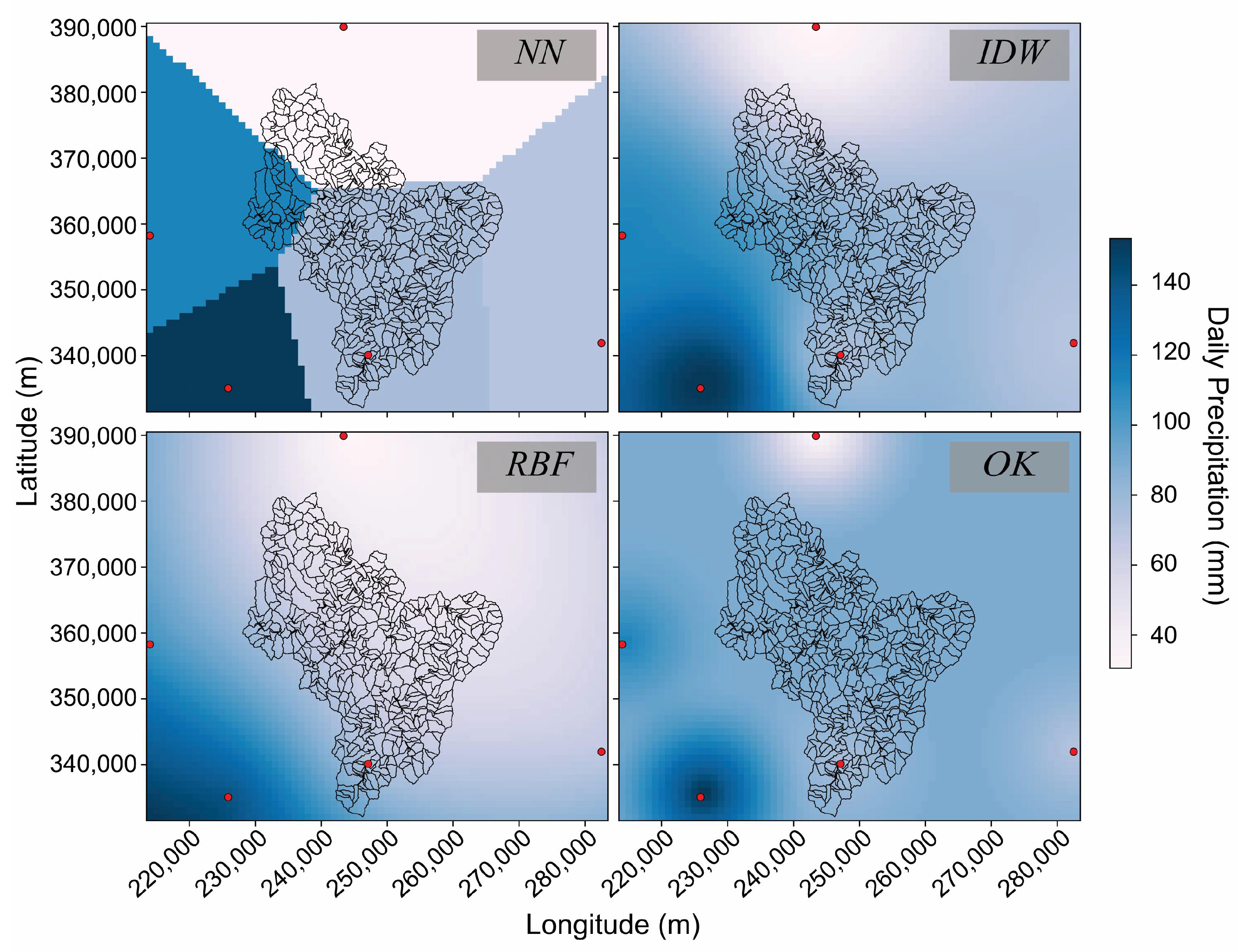
In this study, four interpolation methods, three deterministic methods (i.e., nearest neighbor, radial basis function, inverse-distance-weight), and one geospatial (i.e., ordinary kriging) method, were utilized to determine which spatial interpolation method results in the optimal simulation of daily streamflow in the study area. The visual comparison between the interpolation methods analyzed in this study is shown in Figure 1.
The general formula for all spatial interpolation methods is given as [16]:
where is the interpolated value at an unknown point , is the calculation weight at station , and is the observed value at station , and is the total number of stations. The formula for each interpolation varies depending on how the weights are computed [16].
2.3.1. Nearest Neighbor (NN)
The NN method is the default method utilized within SWAT, which assumes that the precipitation between two stations is linear. NN assigns values to an unknown point, , based on a known value, from the nearest observation point.
2.3.2. Inverse-Distance-Weighting Method (IDW)
IDW is a deterministic method [17] known for its simplicity and widespread applicability [16]. This method assigns interpolated values to unsampled points based on the weighted average of all observed values from known observation stations. Moreover, the interpolated value at an unsampled point is mostly influenced by the nearest observation station, and hence is least influenced by the farthest station. The general formula for IDW is identical to Equation (1), and the weight is given as:
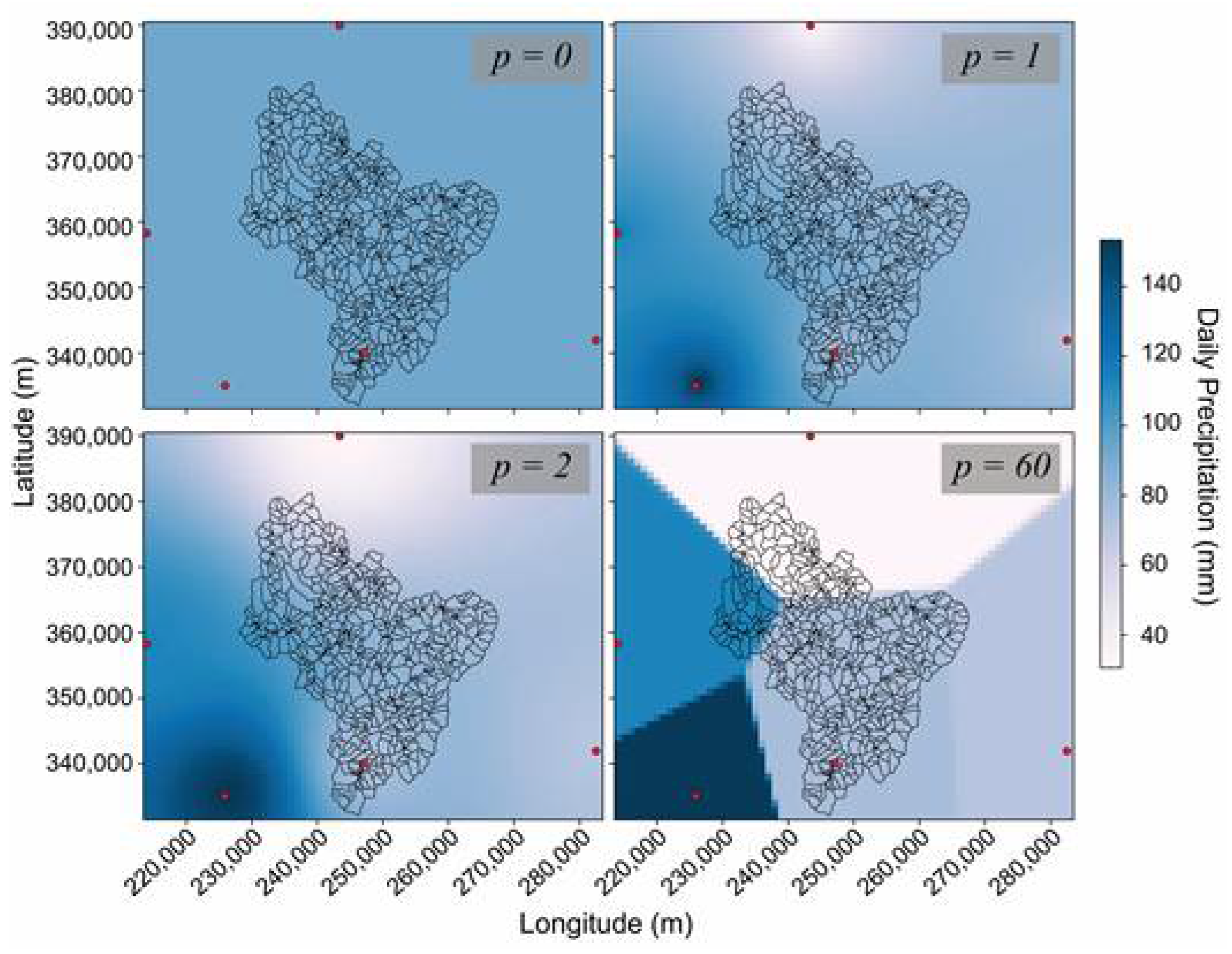
where, is the distance from the unsampled point to the observation station, and is the power value; the power value used in this study is , which has been widely applied on the spatial interpolation of precipitation [3,4,6,7,9,18,19]. The smoothness of the interpolated map depends on the value of . If , the interpolated map will only return the mean value of all observed values; and as the value of increases, the interpolated values at unsampled points will be more localized. If the value of reaches its maximum value, the resulting spatial map will be similar with the NN map (Figure 1). The comparison of IDW maps based on various powers for the same event is shown in Figure 2.
2.3.3. Radial Basis Function (RBF)
RBF is similar to IDW in terms of its simplicity and wide applicability in various fields such as: rainfall-runoff modeling [20,21], flood prediction [22], weather forecasting [23], and estimating precipitation [24,25,26]. The general equation for RBF is given as follows:
wherein, is the radial function; is the weight at ; and is the Euclidean distance between the unknown point and known point . In this study, the linear radial function was utilized for all interpolations, and is given as [27]:
2.3.4. Ordinary Kriging
The ordinary kriging (OK) method is a geostatistical interpolation method that minimizes the variance, and generates unbiased interpolations. Among the various types of Kriging, OK has been frequently used to interpolate daily precipitation inputs in SWAT to improve daily streamflow simulations [3,4,6].
wherein is the partial sill, is the lag-time, is the range, and is the nugget of the semi-variogram.
In this study, the ordinary kriging function from the third-party Python library known as PyKrige [28] was utilized to interpolate daily precipitation inputs.
2.4. Cross-Validation
To determine the accuracy of the model in simulating daily streamflow based on spatially varied precipitation inputs, the simulated daily streamflow was compared with the observed daily streamflow. To quantify the results, two performance indicators were calculated: (1) Nash–Sutcliffe efficiency (NSE) coefficient; (2) root-mean-square error (RMSE).
The Nash–Sutcliffe efficiency coefficient was utilized to determine whether the simulated values can accurately replicate the observed daily streamflow or not. Meanwhile, RMSE was utilized to determine how far the residuals are located from the regression line of data points; it measures the goodness-of-fit of the simulated values with the observed data. NSE values may range from to 1, and RMSE ranges from 0 to . A simulation with NSE = 1, and RMSE = 0, implies an optimal simulation. This study will follow the NSE classifications suggested by Moriasis et al. [29]: very good performance ; good performance ; satisfactory performance ; unsatisfactory performance ; and unacceptable performance . The NSE, and RMSE equations are given as follows:
wherein, the is the number of samples, and corresponds to the mean observed and simulated streamflow, respectively; and and corresponds to the observed and simulated streamflow at iteration, respectively.
2.5. Study Area, Data, and Methodology
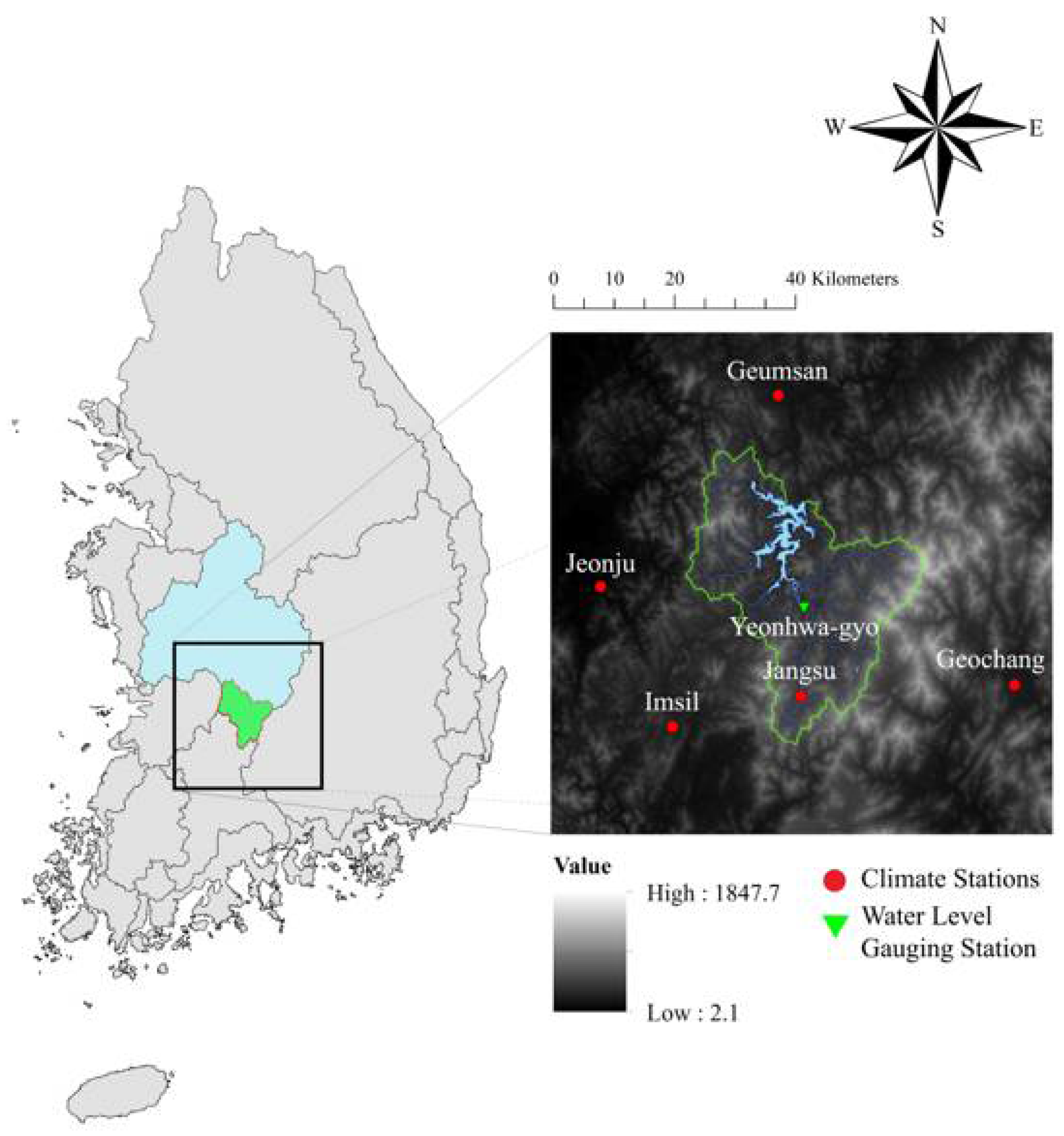
The Yongdam watershed has a catchment size of 930 km2, which is classified as a medium-sized catchment, according to Singh [30]. The min, mean, and max elevations of the basin are 204 m, 525 m, and 1608 m, respectively; with a standard deviation of 207 m, implying that the elevations over the whole basin vary significantly. Furthermore, the basin is situated in the upstream part of the Geum River basin in South Korea, as shown in Figure 3.
Situated between the latitudes of 35.514° to 36.106°, the Yongdam watershed lies within the temperate zone, with cold and dry winters, and hot and humid summers which is further characterized by excessive precipitation during monsoon season locally known as ‘Jangma’ season. Based on the 33 years of precipitation data at Jangsu station (1988 to 2020), the average annual precipitation of the catchment is 1373.44 mm, with an average number of wet days of 150 days, and an average temperature of 11.3 °C [31].
The available daily precipitation, minimum and maximum temperatures, relative humidity, wind speed, and solar radiation data from five nearby automated surface observing systems (ASOS) stations, from the years 2000 to 2020, were obtained from Korea Meteorological Agency (KMA; www.kma.go.kr; accessed on 1 June 2021) database. Table 1 summarizes the detailed information of the five ground observation stations utilized in this study. Based on the annual average precipitations summarized, Jeonju and Jangsu stations had the lowest and highest annual average precipitations, which are also located at the lowest and highest elevations; suggesting that orographic precipitation exists in these areas.
SWAT is a hydrological model that requires a warm-up period, and thus the first four years (2000–2003) were assigned as a warm-up period, while the remaining 17 years (2004–2020) were analyzed in this study. Furthermore, the observed streamflow data at the Yeonhwa-gyo gauging station from the year 2004 to 2020 was retrieved from the Geum River Flood Control Office database (www.geumriver.go.kr; accessed on 1 July 2021), necessary to verify the model outputs. Finally, three required geographic information system (GIS) maps, the digital elevation map (DEM), soil classification map, and land use cover map, were utilized in SWAT.
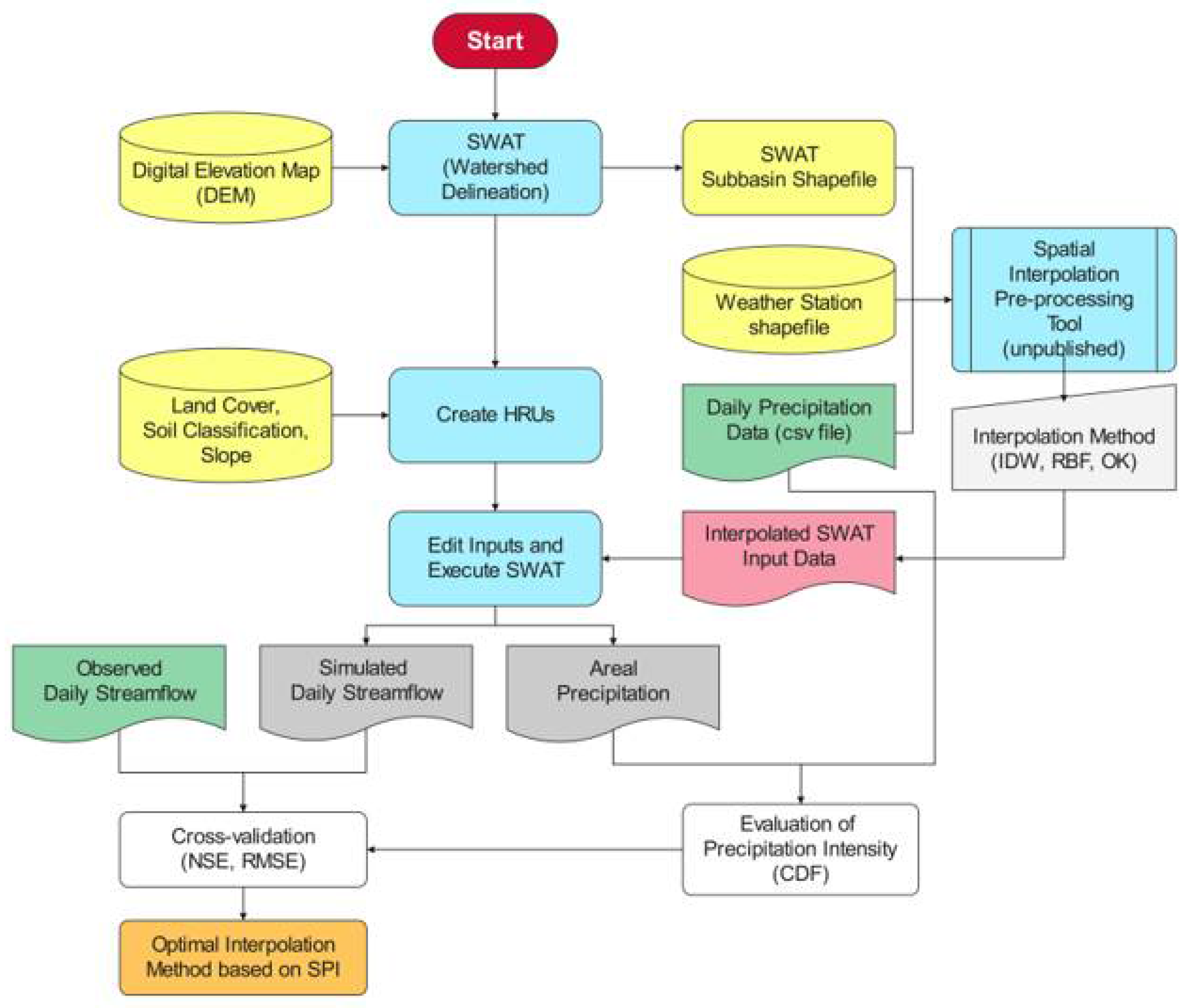
Figure 4 shows the step-by-step procedures of the proposed research methodology. SWAT has three steps: water delineation; creating HRUs; and selecting weather inputs, and program execution.
First, the DEM was utilized to delineate the stream network of the basin. Cho et al. [1] found that maximizing the number of subbasins improves the capabilities of SWAT to simulate daily streamflow. The number of subbasins can be maximized by reducing the defined threshold value when delineating the stream network. In this study, the defined threshold value utilized to delineate the stream network was set to 1 km2, thus resulting in 544 subbasins in total; the delineated subbasin generated is in a form of a shapefile.
For the second step, SWAT disintegrates the subbasins to form HRUs, based on user-specified settings. After completing the first two steps, the spatial interpolation pre-processing tool was utilized to create weather inputs based on the interpolation method selected by the user. The process of creating SWAT inputs was repeated until the SWAT inputs based on all three interpolation methods were completely generated.
The spatial interpolation tool requires two shapefiles (i.e., a subbasin shapefile generated from the first step, and a weather station shapefile that includes the latitude, longitude, and elevation information of each weather station); and one comma-separated values (CSV) file of the observed precipitation data from all stations. After executing the tool, the following files will be generated: (1) subbasin centroid information input file, which replaces the station information input file; and (2) spatially interpolated precipitation time series at each subbasin centroid. These data were used as input data for the third step in SWAT. Finally, the daily streamflow predictions were generated by executing SWAT.
The resulting streamflow and areal precipitations for each case (i.e., interpolation method), were further evaluated and analyzed in this study. First, the cumulative density function (CDF) curves of all four cases (i.e., default NN method, IDW, RBF, and OK) were compared in order to evaluate the difference in precipitation intensities derived from each case. For standardization, the precipitation intensities analyzed were based on the classifications recommended by the World Meteorological Organization (WMO) [13]. Though the unit of intensity originally recommended by the WMO was based on the mm/hour unit, several researchers have successfully applied the same ranges on a daily temporal scale (i.e., mm/day) [9,32]. The WMO classifications adopted in this study are as follows: (1) daily precipitation for no precipitation; (2) daily precipitation for heavy precipitation; and (3) daily precipitation for extreme precipitation events [13].
Finally, the simulated daily streamflow for all four cases was cross-validated by comparing the simulated results with the observed streamflow records, by calculating the NSE and RMSE values for each case. The results of the cross-validation were utilized to determine the optimal interpolation method according to the meteorological conditions of the basin. In this study, the standardized precipitation index recommended by WMO for drought assessments [33], was utilized to identify the long-term meteorological conditions at the Yongdam watershed; the SPI–12 at the study area that has been previously presented by Moazzam et al. [34] was applied in this study. The SPI–12 index [34] at the Yongdam watershed and its respective classification (henceforth, called meteorological conditions) according to WMO [33] are summarized in Table 2.
3. Results and Discussion
3.1. Comparison of Daily Areal Precipitations Based on Different Spatial Interpolation Methods
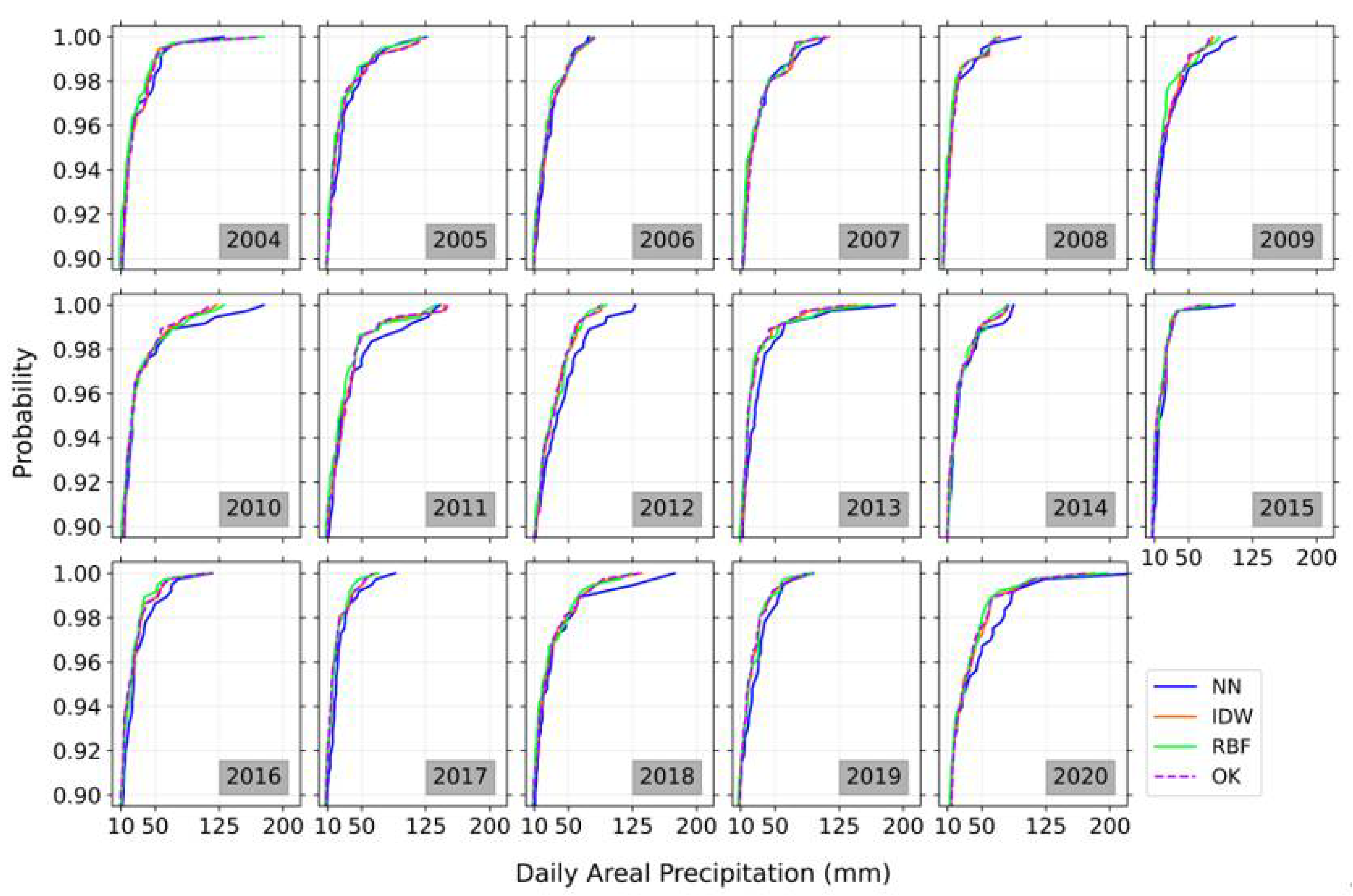
The CDF graphs at Geumsan, Geochang, Imsil, Jangsu, and Jeonju gauging stations (Figure 5) were compared with the CDF graphs of NN-, IDW-, RBF-, and OK-based areal precipitations (Figure 6) to determine which from the observed gauging stations has the most influence on the generated areal precipitations. The NN-based areal precipitations for all cases (Figure 6) were observed to be highly identical to the CDF curve at Jangsu station (Figure 5), which suggests that the NN-based areal precipitation, also the default method used within SWAT, lacks spatial variability over the basin as it solely considers the data from the nearest station and, hence, ignoring the influence of surrounding stations. On the contrary, the CDF curves of IDW-, RBF-, and OK-based areal precipitations were observed to be bounded by the CDF curves of Geumsan, Imsil, Jangsu, and Jeonju gauging stations, suggesting that the areal precipitation generated based on aforementioned method is influenced by the said stations.
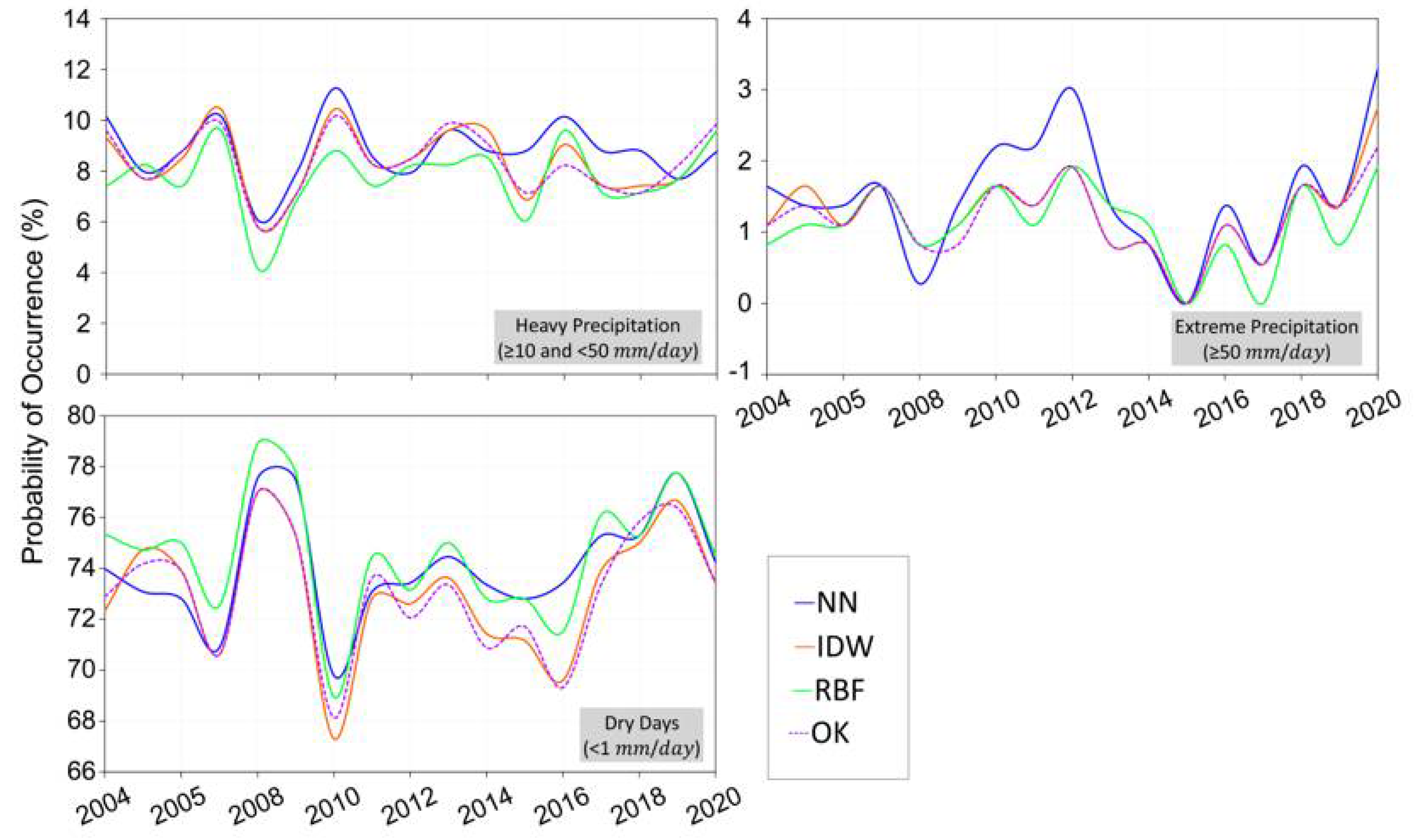
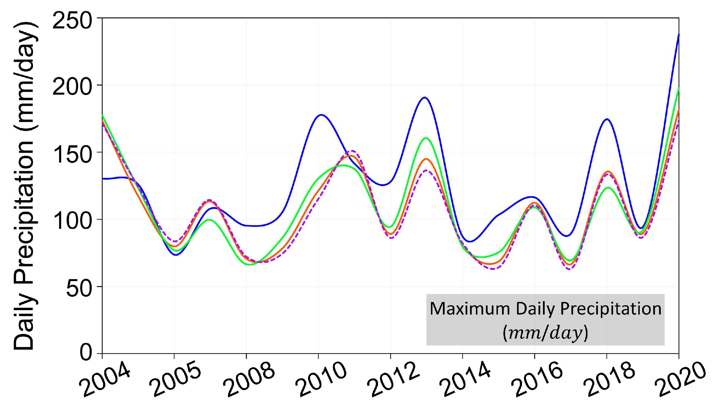
The comparison of occurrence probabilities for various precipitation intensities based on NN-, IDW-, RBF-, and OK-based areal precipitations are shown in Figure 7. NN was observed with the greatest number of days with heavy to extreme () precipitations. Moreover, NN-based precipitation was also observed with the highest magnitude at 100th percentile (i.e., maximum daily precipitation) compared with the other methods shown in Figure 8, thus suggesting that the NN-based precipitation can generate higher flood peaks in the study area.
On the contrary, RBF was observed with the greatest number of dry days , and the least number of days with heavy to extreme () precipitations for majority of the years. Based on these findings, RBF-based daily precipitation is characterized by the least number of wet days, and the least number of days with heavy to extreme precipitations, which can generate lower flood peaks.
The OK-based precipitation was observed with the least number of dry days (i.e., the highest number of wet days), and had the lowest magnitude at 100th percentile (Figure 8) in majority of the years. Based on these results, the daily streamflow that can be generated from utilizing the OK-based daily precipitation will likely results in higher baseflow rates, and lowest peak rates as compared with the other methods. Meanwhile, IDW-based precipitation either had the same or similar results with OK, suggesting similar performance. Ly et al. [16] presented similar findings stating that in terms of hydrological modeling, the streamflow derived from using IDW and geostatistical methods on precipitation data produces comparable results.
3.2. Comparison of Daily Streamflow Based on Different Spatial Interpolation Methods
To quantify the performance of SWAT in simulating daily streamflow based on various precipitation inputs, the NSE and RMSE values are summarized in Table 3. The overall accuracy of SWAT in simulating daily streamflow greatly increased through the utilization of spatial interpolation methods on precipitation inputs, wherein the NSE values increased and the RMSE values decreased.
The default daily simulations (i.e., NN) performed worst in majority of the cases and only outperformed all the other methods in three instances, two when the SPI–12 classification falls under moderately wet conditions (i.e., 2011 and 2020), and one under wet conditions (i.e., 2004; the preceding year 2003 is classified under extremely wet conditions [34]). In addition, during 2004, 2011, and 2020, the NN-based areal precipitation was observed with the highest occurrence probability of extreme precipitation, which is contrary to the findings presented by Cheng et al. [7], who presented that NN-based precipitation performed best for light precipitation patterns. The contradictory in the results can be attributed to the difference in station densities for both studies.
IDW resulted in an overall average performance, neither having the best nor the worst results, regardless of the long-term meteorological conditions of the watershed. It was also observed that most of the IDW results were similar with the results of OK, and vice-versa despite the two methods having different classifications (i.e., deterministic and geospatial methods). Ly et al. [16] reviewed the past literature regarding the performance of using deterministic methods against the geostatistical methods in interpolating daily precipitation inputs in hydrological models, and concluded that while the latter outperformed the former in general, both types of interpolation methods generated comparable results. Moreover, recent researchers [2,35] also concluded the similarity in the streamflow outputs from utilizing IDW and OK interpolated daily precipitation inputs in hydrological models. Dirks et al. [19] also found similar findings, and emphasized that the lack in significant improvements from using OK was due to the limited coverage of semi-variograms. Likewise, in the case of results presented in this study, the coverage of semi-variogram of OK were insufficient to contribute significant influence in areal precipitations; the shortest distance between two gauging stations is approximately 21 km (Imsil to Jangsu station).
While the overall model performance of the model to simulate daily streamflow even pre-model calibration was definitely improved, the NSE values during 2015 (i.e., severely dry) were particularly different. Though the NSE values from IDW, RBF, and OK methods increased as compared with the default NN method, the negative NSE values still implies unacceptable performance. Though both years 2008 and 2015 were classified under severely dry conditions, the former was preceded by wet conditions, while the latter was preceded by dry conditions. Since the model performance for both years improved with RBF precipitation inputs, the feasibility that the other model parameters such as the soil moisture, groundwater, and etc., are the cause of persistent negative NSE values during 2015. Kim and Kim [36] who examined the performance of SWAT in simulating daily streamflow during long-term drought periods (i.e., 2014–2015) at a medium-sized watershed in Korea found out that the modification (calibration) of nine SWAT parameters (i.e., maximum canopy storage, CANMX; SCS curve number, CN2; soil evaporation compensation coefficient, ESCO; saturated hydraulic conductivity, SOL_K; slope length of lateral subsurface flow, SLSOIL; lateral flow travel time, LAT_TTIME; delay time for aquifer recharge, GW_DELAY; threshold water level in shallow aquifer for base flow, GWQMN; and baseflow recession coefficient, ALPHA_BF) greatly improved the model performance (i.e., NSE values) from unacceptable to satisfactory results.
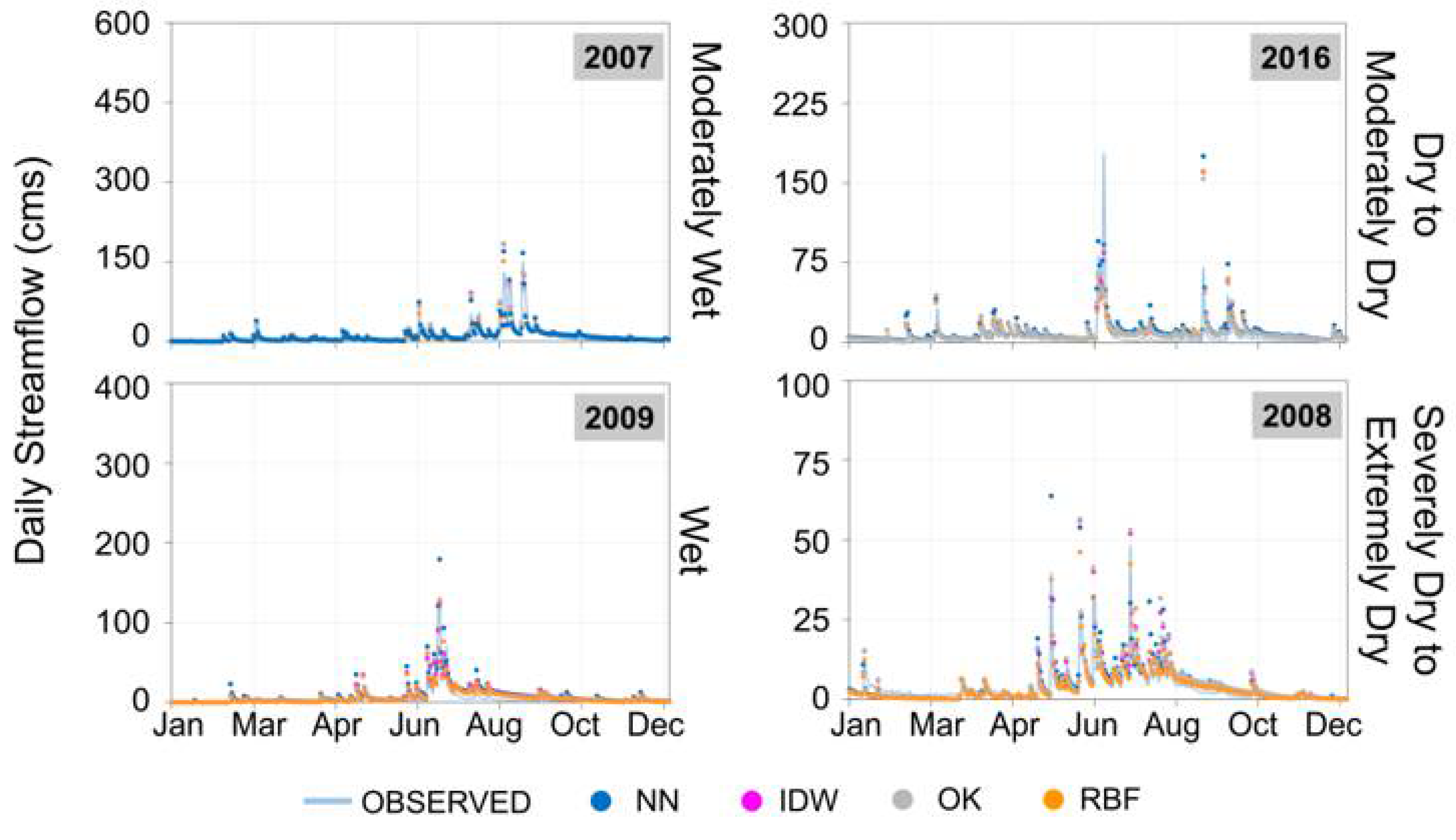
To summarize the performance of each spatial interpolation method on daily streamflow predictions in the study area, NN-(RBF-) based daily precipitation most likely results in higher (lower) flood peaks, and both OK- and IDW-based daily precipitation had the tendency to generate higher baseflow rates and lowest peak rates as compared with the other interpolation methods as shown in Figure 9.
Finally, the comparison between the observed and simulated daily streamflow grouped according to SPI–12 classifications and the optimal interpolation method for each case at the Yongdam dam basin are summarized as follows: for moderately wet conditions, NN performed best; RBF for wet, severely dry, and extremely dry conditions; and OK or IDW for dry to moderately dry conditions.
Finally, RBF performed well in majority of the cases, resulting to decreased RMSE, and improved NSE (i.e., from satisfactory to very good), regardless of the meteorological conditions of the basin. However, it was also observed that RBF particularly performed best during wet conditions, and during severely dry to extremely dry conditions, except during 2015. The characteristics of RBF-based precipitation (i.e., the greatest number of dry days, least number of wet days, least number of days with heavy to extreme precipitations) matches the dry conditions in terms of having lower baseflow rates, and lower flood peaks, as compared with the other methods.
4. Conclusions
This study aims to improve the research gaps in existing methodologies on the improvement of SWAT precipitation inputs in simulating daily streamflow at the Yongdam watershed, with the following detailed objectives: (1) to evaluate the applicability of the pre-processing tool to generate daily precipitation inputs; (2) to determine the applicability of each interpolation method based on WMO classifications of precipitation intensities; and (3) to analyze the impacts of various spatial interpolation methods on daily streamflow predictions with SWAT even pre-model calibration. The key findings presented in this study are summarized as follows:
- –
- The spatial interpolation pre-processing presented in this study improved the overall productivity of interpolating long-term daily precipitation datasets as SWAT inputs. Furthermore, the interpolation methods (i.e., default NN, IDW, RBF, and OK methods) included within the tool were also proven to increase the prediction efficiencies of SWAT to simulate daily streamflow at the Yongdam watershed, even pre-model calibration;
- –
- The applicability of interpolation methods based on the precipitation intensities at the Yongdam watershed, standardized by the World Meteorological Organization [13] are as follows: (1) NN outperformed the other methods in few cases when the occurrence probability of extreme precipitation is high, during wet to moderately wet conditions; (2) RBF-based outperformed the other methods for cases when the number of dry days were high, with minimum number of days with heavy to extreme precipitations;
- –
- Among the methods utilized, the precipitation generated from utilizing RBF mostly outperformed the other methods regardless of the meteorological conditions at the study area;
- –
- Even pre-model calibration, the daily streamflow predictions with SWAT were improved through the use of interpolation methods. However, for cases when long-term drought occurs, the surface, subsurface, and groundwater parameters of the model should be calibrated to improve the daily streamflow predictions;
- –
- The peak flow rates at the study area were found to be sensitive to the type of interpolation methods utilized;
- –
- The selection of the optimal interpolation method at Yongdam watershed can be based on both the meteorological conditions (i.e., SPI) and the precipitation intensities at Yongdam watershed. Thus, the selection of a single method to interpolate the long-term daily precipitation inputs in SWAT, will not result in optimal performance. However, it was also observed that the RBF method outperformed the other methods in majority of the cases based on the meteorological conditions;
- –
- Therefore, based on the results presented in this research, the optimal spatial interpolation method at the Yongdam watershed based on the meteorological conditions of the basin are as follows: NN for moderately wet conditions; RBF for wet, severely dry, and extremely dry conditions; and OK or IDW for dry to moderately dry conditions;
- –
- This study utilized a pre-calibrated model to isolate the effects of interpolation methods from other model parameters, and thus the resulting streamflow cannot be applied to practice (i.e., watershed management, dam operations, and sediment analysis). For practical applications, the model should be calibrated after selecting the best interpolation method for precipitation;
- –
- Finally, the methodology presented in this study was applied to the Yongdam watershed, a medium-sized catchment with complex terrain characteristics (i.e., mountainous). However, due to the complexity of its topography, limitations must be considered in yielding generalized findings. Therefore, it is suggested that this methodology be applied to several catchments with different terrain characteristics to determine the applicability of the methodology even for various catchments;
- –
- The methodology and tool proposed in this study can serve as a means to further understand how spatial interpolation methods affect the daily streamflow predictions at the Yongdam watershed.
Author Contributions
Conceptualization, methodology, software, validation, formal analysis, resources, data curation, writing—original draft preparation, writing—review and editing, M.L.F.; funding acquisition, K.J. All authors have read and agreed to the published version of the manuscript.
Funding
This research was supported and funded by the National Research Foundation of Korea, 2019K1A3A1A05087901.
Institutional Review Board Statement
Not applicable.
Informed Consent Statement
Not applicable.
Data Availability Statement
The daily precipitation, daily minimum temperature, and daily maximum temperature used in this study has been obtained from the Korea Meteorological Agency database accessible after login at https://data.kma.go.kr/ (accessed on 1 June 2021). The spatial interpolation pre-processing tool will be available upon request through the following E-mail address: ([email protected]).
Acknowledgments
The authors would like to thank Lea Dasallas for providing constructive comments to improve the contents of this paper.
Conflicts of Interest
The authors declare no conflict of interest. The funders had no role in the design of the study; in the collection, analyses, or interpretation of data; in the writing of the manuscript, or in the decision to publish the results.
References
- Cho, J.; Bosch, D.; Lowrance, R.; Strickland, T.; Vellidis, G. Effect of Spatial Distribution of Rainfall on Temporal and Spatial Uncertainty of SWAT Output. Trans. ASABE 2009, 52, 1545–1556. [Google Scholar] [CrossRef]
- Masih, I.; Maskey, S.; Uhlenbrook, S.; Smakhtin, V. Assessing the Impact of Areal Precipitation Input on Streamflow Simulations Using the SWAT Model. J. Am. Water Resour. Assoc. 2011, 47, 179–195. [Google Scholar] [CrossRef]
- Zeiger, S.; Hubbart, J. An assessment of mean areal precipitation methods on simulated stream flow: A SWAT model performance assessment. Water 2017, 9, 459. [Google Scholar] [CrossRef] [Green Version]
- Van Der Heijden, S.; Haberlandt, U. Influence of spatial interpolation methods for climate variables on the simulation of discharge and nitrate fate with SWAT. Adv. Geosci. 2010, 27, 91–98. [Google Scholar] [CrossRef] [Green Version]
- Abbas, S.A.; Xuan, Y. Impact of Precipitation Pre-Processing Methods on Hydrological Model Performance using High-Resolution Gridded Dataset. Water 2020, 12, 840. [Google Scholar] [CrossRef] [Green Version]
- Szcześniak, M.; Piniewski, M. Improvement of Hydrological Simulations by Applying Daily Precipitation Interpolation Schemes in Meso-Scale Catchments. Water 2015, 7, 747–779. [Google Scholar] [CrossRef] [Green Version]
- Cheng, M.; Wang, Y.; Engel, B.; Zhang, W.; Peng, H.; Chen, X.; Xia, H. Performance assessment of spatial interpolation of precipitation for hydrological process simulation in the Three Gorges Basin. Water 2017, 9, 838. [Google Scholar] [CrossRef] [Green Version]
- Jang, D.; Kim, D.; Kim, Y.; Choi, W. Application of SWAT Model considering Spatial Distribution of Rainfall. J. Wetlands Res. 2018, 20, 94–103. [Google Scholar] [CrossRef]
- Tuo, Y.; Duan, Z.; Disse, M.; Chiogna, G. Evaluation of precipitation input for SWAT modeling in Alpine catchment: A case study in the Adige river basin (Italy). Sci. Total Environ. 2016, 573, 66–82. [Google Scholar] [CrossRef] [PubMed] [Green Version]
- Arnold, J.G.; Moriasi, D.N.; Gassman, P.W.; Abbaspour, K.C.; White, M.J.; Srinivasan, R.; Santhi, C.; Harmel, R.D.; van Griensven, A.; Van Liew, M.W.; et al. SWAT: Model Use, Calibration, and Validation. Trans. ASABE 2012, 55, 1491–1508. [Google Scholar] [CrossRef]
- Neitsch, S.; Arnold, J.; Kiniry, J.; Williams, J. Soil & Water Assessment Tool Theoretical Documentation Version 2009; Texas Water Resources Institute: College Station, TX, USA, 2011. [Google Scholar]
- Thiessen, A.H. Precipitation Averages for Large Areas. Mon. Weather Rev. 1911, 39, 1082–1089. [Google Scholar] [CrossRef]
- World Meteorological Organization. Volume I—Measurement of Meteorological Variables; World Meteorological Organization: Geneva, Switzerland, 2018; Volume I, ISBN 978-92-63-10008-5. [Google Scholar]
- Sharpley, A.N.; Williams, J. EPIC-Erosion/Productivity Impact Calculator: 1. Model Documentation; US Department of Agriculture: Washington, DC, USA, 1990.
- Schuol, J.; Abbaspour, K.C. Using monthly weather statistics to generate daily data in a SWAT model application to West Africa. Ecol. Model. 2007, 201, 301–311. [Google Scholar] [CrossRef]
- Ly, S.; Charles, C.; Degré, A. Different methods for spatial interpolation of rainfall data for operational hydrology and hydrological modeling at watershed scale. A review. Biotechnol. Agron. Soc. Environ. 2013, 17, 392–406. [Google Scholar]
- Shepard, D. A two-dimensional interpolation function for irregularly-spaced data. In Proceedings of the 1968 23rd ACM National Conference; ACM Press: New York, NY, USA, 1968; pp. 517–524. [Google Scholar]
- Charles, T.H. Statistical Methods in Hydrology, 2nd ed.; Wiley: Hoboken, NJ, USA, 2002; ISBN 9780813815039. [Google Scholar]
- Dirks, K.N.; Hay, J.E.; Stow, C.D.; Harris, D. High-resolution studies of rainfall on Norfolk Island. J. Hydrol. 1998, 208, 187–193. [Google Scholar] [CrossRef]
- Lin, G.-F.; Chen, L.-H. A non-linear rainfall-runoff model using radial basis function network. J. Hydrol. 2004, 289, 1–8. [Google Scholar] [CrossRef]
- Suhaimi, S.; Bustami, R.A. Rainfall Runoff Modeling using Radial Basis Function Neural Network for Sungai Tinjar Catchment, Miri, Sarawak. J. Civ. Eng. Sci. Technol. 2009, 1, 1–7. [Google Scholar] [CrossRef] [Green Version]
- Panigrahi, B.K.; Nath, T.K.; Senapati, M.R. An application of local linear radial basis function neural network for flood prediction. J. Manag. Anal. 2019, 6, 67–87. [Google Scholar] [CrossRef]
- Santhanam, T.; Subhajini, A.C. An Efficient Weather Forecasting System using Radial Basis Function Neural Network. J. Comput. Sci. 2011, 7, 962–966. [Google Scholar] [CrossRef] [Green Version]
- Antal, A.; Guerreiro, P.M.P. A radial basis function approach to estimate precipitations in Brasov County, Romania. Environ. Eng. Manag. J. 2021, 20, 1383–1394. [Google Scholar] [CrossRef]
- Auzani, H.; Has-Yun, K.S.; Nazri, F.A.M. Development of Trees Management System Using Radial Basis Function Neural Network for Rain Forecast. Comput. Water Energy Environ. Eng. 2022, 11, 1–10. [Google Scholar] [CrossRef]
- Luo, X.; Xu, Y.; Xu, J. Application of Radial Basis Function Network for spatial precipitation interpolation. In Proceedings of the 2010 18th International Conference on Geoinformatics, Beijing, China, 18–20 June 2010; pp. 1–5. [Google Scholar]
- Dehghan, M.; Shafieeabyaneh, N. Local radial basis function–finite-difference method to simulate some models in the nonlinear wave phenomena: Regularized long-wave and extended Fisher–Kolmogorov equations. Eng. Comput. 2021, 37, 1159–1179. [Google Scholar] [CrossRef]
- Murphy, B.; Müller, S.; Yurchak, R. GeoStat-Framework/PyKrige: v1.6.1.; Zenodo: Genève, Switzerland, 2021. [Google Scholar]
- Moriasi, D.N.; Arnold, J.G.; Van Liew, M.W.; Bingner, R.L.; Harmel, R.D.; Veith, T. Model Evaluation Guidelines for Systematic Quantification of Accuracy in Watershed Simulations. Trans. ASABE 2007, 50, 885–900. [Google Scholar] [CrossRef]
- Singh, V.P. Chapter 1: Watershed Modelling. In Computer Models of Watershed Hydrology; Water Resources Publications: Littleton, CO, USA, 1995. [Google Scholar]
- Felix, M.L.; Kim, Y.; Choi, M.; Kim, J.; Do, X.K.; Nguyen, T.H.; Jung, K. Detailed Trend Analysis of Extreme Climate Indices in the Upper Geum River Basin. Water 2021, 13, 3171. [Google Scholar] [CrossRef]
- Wang, W.; Hocke, K.; Mätzler, C. Physical Retrieval of Rain Rate from Ground-Based Microwave Radiometry. Remote Sens. 2021, 13, 2217. [Google Scholar] [CrossRef]
- World Meteorological Organization; Svoboda, M.; Hayes, M.; Wood, D.A. Standardized Precipitation Index User Guide; World Meteorological Organization: Geneva, Switzerland, 2012. [Google Scholar]
- Moazzam, M.F.U.; Rahman, G.; Munawar, S.; Farid, N.; Lee, B.G. Spatiotemporal Rainfall Variability and Drought Assessment during Past Five Decades in South Korea Using SPI and SPEI. Atmosphere 2022, 13, 292. [Google Scholar] [CrossRef]
- Ruelland, D.; Ardoin-Bardin, S.; Billen, G.; Servat, E. Sensitivity of a lumped and semi-distributed hydrological model to several methods of rainfall interpolation on a large basin in West Africa. J. Hydrol. 2008, 361, 96–117. [Google Scholar] [CrossRef]
- Kim, D.R.; Kim, S.J. A Study on Parameter Estimation for SWAT Calibration Considering Streamflow of Long-term Drought Periods. J. Korean Soc. Agric. Eng. 2017, 59, 19–27. [Google Scholar] [CrossRef]
Figure 1.
Comparison of all spatial interpolation methods utilized in this study (red markers show the location of all observation stations considered) for the same event.
Figure 1.
Comparison of all spatial interpolation methods utilized in this study (red markers show the location of all observation stations considered) for the same event.

Figure 2.
The visual comparison of IDW maps based on various powers () for the same event.

Figure 3.
Location of the Yongdam watershed (green) in Geum River Basin (blue) and the location of all climate, and water level gauging stations utilized in this study.
Figure 3.
Location of the Yongdam watershed (green) in Geum River Basin (blue) and the location of all climate, and water level gauging stations utilized in this study.

Figure 4.
Flowchart of research methodology.

Figure 5.
Occurrence frequencies of daily precipitation intensities observed at Geumsan, Geochang, Imsil, Jangsu, and Jeonju gauging stations from the year 2004 to 2020.
Figure 5.
Occurrence frequencies of daily precipitation intensities observed at Geumsan, Geochang, Imsil, Jangsu, and Jeonju gauging stations from the year 2004 to 2020.

Figure 6.
Comparison of occurrence frequencies of daily areal precipitation intensities based on four spatial interpolation methods from the year 2004 to 2020.
Figure 6.
Comparison of occurrence frequencies of daily areal precipitation intensities based on four spatial interpolation methods from the year 2004 to 2020.

Figure 7.
Probability of occurrence of dry days, days with heavy precipitation, and days with extreme precipitations based on the default NN-, IDW-, RBF-, and OK-based areal precipitations.
Figure 7.
Probability of occurrence of dry days, days with heavy precipitation, and days with extreme precipitations based on the default NN-, IDW-, RBF-, and OK-based areal precipitations.

Figure 8.
Maximum daily precipitation per year based on the NN-, IDW-, RBF-, and OK-based areal precipitations.
Figure 8.
Maximum daily precipitation per year based on the NN-, IDW-, RBF-, and OK-based areal precipitations.

Figure 9.
Optimal interpolation method based on long-term meteorological conditions at the Yongdam watershed (NN for moderately wet, OK or IDW for dry to moderately dry, and RBF for wet or severely dry to extremely dry conditions).
Figure 9.
Optimal interpolation method based on long-term meteorological conditions at the Yongdam watershed (NN for moderately wet, OK or IDW for dry to moderately dry, and RBF for wet or severely dry to extremely dry conditions).


Table 1.
Detailed information of weather stations utilized in this study.
| No. | Station Name | Longitude °E | Latitude °N | Elevation (m. a. s. l.) | Annual Average Precipitation (mm) |
|---|---|---|---|---|---|
| 1 | Jeonju | 127.155 | 35.822 | 61.4 | 1267.5 |
| 2 | Geumsan | 127.482 | 36.106 | 172.69 | 1289.3 |
| 3 | Geochang | 127.909 | 35.667 | 225.95 | 1263.5 |
| 4 | Imsil | 127.286 | 35.612 | 247.04 | 1336.2 |
| 5 | Jangsu | 127.520 | 35.657 | 406.49 | 1476.8 |
| Year | SPI–12 | WMO Classification | Year | SPI–12 | WMO Classification |
|---|---|---|---|---|---|
| 2004 | 0.40 | Wet | 2013 | −1.00 | Moderately Dry |
| 2005 | 0.60 | Wet | 2014 | −0.70 | Dry |
| 2006 | −0.10 | Dry | 2015 | −1.80 | Severely Dry |
| 2007 | 1.40 | Moderately Wet | 2016 | −0.70 | Dry |
| 2008 | −1.50 | Severely Dry | 2017 | −2.00 | Extremely Dry |
| 2009 | 0.25 | Wet | 2018 | −0.20 | Dry |
| 2010 | 1.00 | Wet | 2019 | −0.90 | Dry |
| 2011 | 1.25 | Moderately Wet | 2020 | 1.10 | Moderately Wet |
| 2012 | 0.25 | Wet |
Table 3.
Annual summary of RMSE, and NSE values for daily streamflow simulations based on NN, IDW, RBF, and OK interpolation methods at Yeonhwa-gyo gauging station.
Table 3.
Annual summary of RMSE, and NSE values for daily streamflow simulations based on NN, IDW, RBF, and OK interpolation methods at Yeonhwa-gyo gauging station.
| Year | Meteorological Condition | NSE | RMSE | ||||||||||||
|---|---|---|---|---|---|---|---|---|---|---|---|---|---|---|---|
| NN | IDW | RBF | OK | NN | IDW | RBF | OK | ||||||||
| 2004 | Wet | 0.70 | ▽ | 0.35 | ▽ | 0.59 | ▼ | 0.22 | 9.41 | △ | 13.84 | △ | 11.03 | ▲ | 15.19 |
| 2005 | Wet | 0.85 | ▲ | 0.87 | △ | 0.83 | ▲ | 0.87 | 8.25 | ▼ | 7.42 | ▲ | 8.62 | ▽ | 7.49 |
| 2006 | Dry | 0.72 | ▲ | 0.79 | △ | 0.74 | ▲ | 0.79 | 10.02 | ▼ | 8.71 | ▽ | 9.60 | ▽ | 8.78 |
| 2007 | Moderately Wet | 0.80 | = | 0.80 | ▲ | 0.82 | ▼ | 0.79 | 8.30 | △ | 8.32 | ▼ | 7.97 | ▲ | 8.63 |
| 2008 | Severely Dry | 0.54 | △ | 0.72 | ▲ | 0.82 | △ | 0.64 | 3.66 | ▽ | 2.85 | ▼ | 2.31 | ▽ | 3.27 |
| 2009 | Wet | 0.54 | △ | 0.75 | ▲ | 0.77 | △ | 0.74 | 7.89 | ▼ | 5.84 | ▽ | 5.61 | ▽ | 5.93 |
| 2010 | Wet | 0.74 | △ | 0.84 | ▲ | 0.86 | △ | 0.79 | 11.84 | ▽ | 9.33 | ▼ | 8.61 | ▽ | 10.65 |
| 2011 | Moderately Wet | 0.79 | ▽ | 0.74 | ▼ | 0.70 | ▽ | 0.72 | 16.47 | △ | 18.27 | ▲ | 19.46 | △ | 18.86 |
| 2012 | Wet | 0.70 | △ | 0.73 | ▲ | 0.75 | = | 0.70 | 15.12 | ▽ | 14.43 | ▼ | 13.99 | ▽ | 15.34 |
| 2013 | Moderately Dry | 0.15 | △ | 0.72 | △ | 0.67 | ▲ | 0.79 | 13.25 | ▽ | 7.58 | ▽ | 8.23 | ▼ | 6.58 |
| 2014 | Dry | 0.56 | △ | 0.63 | △ | 0.62 | ▲ | 0.64 | 7.14 | ▽ | 6.62 | ▽ | 6.65 | ▼ | 6.45 |
| 2015 | Severely Dry | −8.54 | △ | −4.84 | ▲ | −3.89 | △ | −4.18 | 5.86 | ▽ | 4.59 | ▼ | 4.20 | ▽ | 4.32 |
| 2016 | Dry | 0.34 | △ | 0.48 | △ | 0.39 | ▲ | 0.55 | 10.74 | ▽ | 9.50 | ▽ | 10.29 | ▼ | 8.81 |
| 2017 | Extremely Dry | −1.27 | △ | 0.00 | ▲ | 0.37 | △ | 0.02 | 7.31 | ▽ | 4.84 | ▼ | 3.84 | ▽ | 4.79 |
| 2018 | Dry | 0.41 | △ | 0.77 | ▲ | 0.79 | △ | 0.78 | 13.43 | ▽ | 8.40 | ▼ | 7.99 | ▽ | 8.26 |
| 2019 | Dry | 0.45 | △ | 0.54 | △ | 0.53 | ▲ | 0.55 | 7.72 | ▽ | 7.04 | ▽ | 7.07 | ▼ | 6.96 |
| 2020 | Moderately Wet | 0.81 | = | 0.81 | ▼ | 0.78 | ▽ | 0.80 | 17.90 | △ | 17.92 | ▲ | 19.06 | △ | 18.48 |
▽(△): lower (higher) values than the default value NN;▼(▲): lowest (highest) value among the results; =: value equal to the default method; bold values represents the best results among the four interpolation methods used.
Publisher’s Note: MDPI stays neutral with regard to jurisdictional claims in published maps and institutional affiliations. |
© 2022 by the authors. Licensee MDPI, Basel, Switzerland. This article is an open access article distributed under the terms and conditions of the Creative Commons Attribution (CC BY) license (https://creativecommons.org/licenses/by/4.0/).
Share and Cite
MDPI and ACS Style
Felix, M.L.; Jung, K. Impacts of Spatial Interpolation Methods on Daily Streamflow Predictions with SWAT. Water 2022, 14, 3340. https://doi.org/10.3390/w14203340
AMA Style
Felix ML, Jung K. Impacts of Spatial Interpolation Methods on Daily Streamflow Predictions with SWAT. Water. 2022; 14(20):3340. https://doi.org/10.3390/w14203340
Chicago/Turabian StyleFelix, Micah Lourdes, and Kwansue Jung. 2022. "Impacts of Spatial Interpolation Methods on Daily Streamflow Predictions with SWAT" Water 14, no. 20: 3340. https://doi.org/10.3390/w14203340
Note that from the first issue of 2016, this journal uses article numbers instead of page numbers. See further details here.