
Assessing the Performance of SHETRAN Simulating a Geologically Complex Catchment

1
Laboratorio de Ecología Acuática (LEA), Facultad de Ciencias Químicas, Universidad de Cuenca, Av. 12 de Abril S/N y Av. Loja, Cuenca 010203, Ecuador
2
Departamento de Ingeniería Civil, Facultad de Ingeniería, Universidad de Cuenca, Av. 12 de Abril S/N y Av. Loja, Cuenca 010203, Ecuador
3
School of Engineering, Newcastle University, Newcastle upon Tyne NE1 7RU, UK
*
Author to whom correspondence should be addressed.
Water 2022, 14(20), 3334; https://doi.org/10.3390/w14203334
Submission received: 23 September 2022
/
Revised: 14 October 2022
/
Accepted: 18 October 2022
/
Published: 21 October 2022
(This article belongs to the Special Issue Decision-Making Theory and Methodology for Water, Energy and Food Security)
Abstract
:Despite recent progress in terms of cheap computing power, the application of physically-based distributed (PBD) hydrological codes still remains limited, particularly, because some commercial-license codes are expensive, even under academic terms. Thus, there is a need for testing the performance of free-license PBD codes simulating complex catchments, so that cheap and reliable mechanistic modelling alternatives might be identified. The hydrology of a geologically complex catchment (586 km2) was modelled using the free-license PBD code SHETRAN. The SHETRAN evaluation took place by comparing its predictions with (i) discharge and piezometric time series observed at different locations within the catchment, some of which were not taken into account during model calibration (i.e., multi-site test); and (ii) predictions from a comparable commercial-license code, MIKE SHE. In general, the discharge and piezometric predictions of both codes were comparable, which encourages the use of the free-license SHETRAN code for the distributed modelling of geologically complex systems.
1. Introduction
Understanding the main physical processes governing the flow dynamics in the land phase of the hydrologic cycle, as well as the consequences of human activities and climatic changes on this cycle is important for integrated catchment management [1]. This is usually facilitated through the use of different water resources codes. The use of physically-based distributed (PBD) hydrologic codes for this purpose is an interesting alternative. In principle, they do not require calibration because their governing equations are based on the physical description of the main hydrological processes and the geographical variation of physical catchment properties can be acceptably represented in them through a spatially distributed grid. In practice, these models (resulting from the site-specific parameterisation of PBD codes) do require calibration for a number of reasons, particularly dealing with [2,3,4] (i) mismatches between the scale at which the code-embedded physical equations were derived, the scale of data acquisition and the scale at which the modelling is taking place (i.e., modelling resolution); and (ii) sub-grid heterogeneity of the model parameter values.
Due to various aspects, among which their complexity is perhaps the principal one, PBD models have usually been calibrated manually (i.e., Refsgaard [2],Vázquez, Feyen, Feyen and Refsgaard [3]). There has been some automatic calibration in PBD applications, although with modelling simplifications, such as, adopting coarse resolutions and considering in detail only surface and subsurface processes [5,6] or even only surface processes in a very simplified manner [7]. Indeed, only a few automatic calibration studies have focused on all the catchment processes including groundwater flow [8]. Even fewer applications have used semi-automatic calibration and considered the multi-dimensional model parameter space, e.g., through Monte Carlo simulations. This is mainly due to the substantial running time associated with the complexity of the models which requires many thousands of simulations [9,10,11,12,13].
Recent growing computational power and extensive surveying/monitoring capacity has ameliorated to a certain extent earlier limitations for a wider use of PBD codes. Nevertheless, the latest applications of this type of codes are mainly of research nature [7,14,15,16] and are still being affected by substantial running times, which is limiting (i) the modelling resolution [14]; (ii) the physical/distributed representation of components of the hydrological cycle [7]; as well as (iii) a wider non-research use of these PBD codes. But it is not only significant running times that are preventing a wider use of this type of codes: expensive commercial-license costs, even at research rates, prevent users from applying these codes. Thus, there is a need for testing the performance of free-license, preferably open source, PBD codes simulating complex catchments, so that, cheap and reliable mechanistic modelling alternatives might be identified.
One of these non-commercial (free-license) PBD codes is SHETRAN [17]. It has been applied for simulating the hydrological dynamics of a variety of catchments [18,19,20,21,22,23,24], although considering only simple representations of the geology of the modelled systems (with no more than two geological layers/aquifers). Further, the assessment of the performance of SHETRAN applications has traditionally been based on the use of a set of multi-objective model performance statistics [6,15,25], often using performance measures that are correlated or are oversensitive to peak flows [6,15,19,26]. Indeed, the complex nature of these PBD codes, and the associated modelling uncertainties [10,11,25,27], requires the consideration of a set of preferably uncorrelated statistics and, in addition, spatially distributed evaluation tests [2,28] that are still uncommon in SHETRAN applications found in the literature.
Hence, with the intention of contributing to increasing the use of free-license codes in water resources assessments, both, in research and consulting projects, the general objective of this research was to evaluate the performance of the PBD free-license code SHETRAN for simulating simultaneously the surface, subsurface and groundwater dynamics of a geologically complex catchment. The research questions were: (i) is it feasible to describe acceptably well within SHETRAN the geometry and main physical variability of a geologically complex study site? (ii) is it possible to run an evaluation protocol, suitable for PBD codes, that can properly characterise the accuracy of SHETRAN predictions? and (iii) is it possible to obtain SHETRAN predictions for a geologically complex study site that are comparable to predictions from a similar commercial-license code? It has to be stressed that the aim of this research was not optimising the modelling of the study site but testing the capability of SHETRAN to perform congruently while simulating geologically complex systems. To the best of our knowledge, this is the first attempt to apply SHETRAN on such a complex non-experimental study site and this through the application of a more robust modelling protocol than most previous research.
2. Materials and Methods
2.1. The Study Site
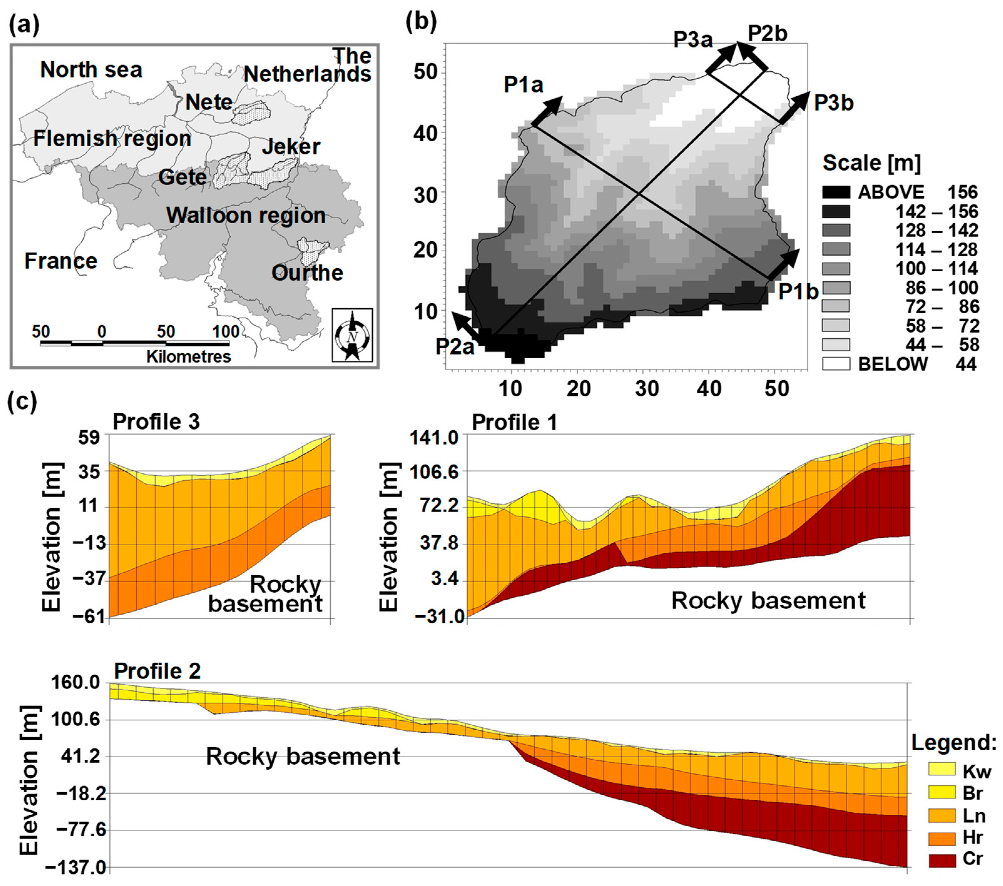
In the forthcoming text only some main characteristics of the study site are listed. Further information can be found in Feyen, et al. [29], Vázquez [9], Vázquez, Feyen, Feyen and Refsgaard [3] and Vázquez and Hampel [12]. The study site is the Gete catchment (586 km2) which is in the central part of Belgium (Figure 1a). The ground elevation (Figure 1b) ranges from approximately 27 m in the north to 174 m in the south. Land use in the area is mainly agricultural, including pasture and cultivated fields, with some local forested patches. Soils have a loamy texture and are deep; nine soil units can be distinguished according to the Belgian soil map. The groundwater table is generally at a depth of 3 to 10 m below surface. The complex lithostratigraphy of the study site comprises nine units, some of which occur only in isolated parts of the catchment. The main units are shown in Figure 1c and this includes a narrow Quaternarian loamy deposit on top of deeper sandy and clayey units resting on top of a low-permeable Palaeozoic rocky basement. The local weather is characterised by moderate humid conditions.
2.2. Hydrological Codes
2.2.1. SHETRAN Hydrological Code
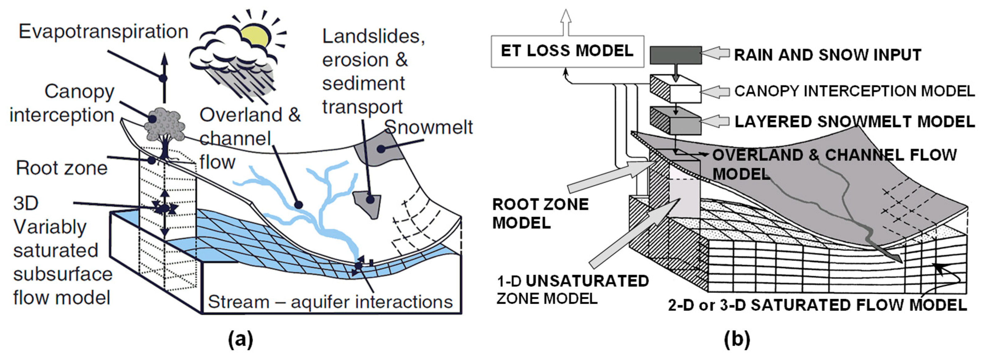
SHETRAN is a PBD code used for the simulation of the land phase of the hydrological cycle and sediment, heat and contaminant transports in river catchments [17,24,30]. The code has a modular structure for simulating each of these components. Simulations are performed by considering the catchment as a set of vertical columns (Figure 2a) with each column divided into finite-difference cells. The lower cells contain aquifer materials and groundwater, higher cells contain soil and soil water and the uppermost cells contain surface waters and the vegetation canopy. The mesh follows the topography of the catchment with channels specified around the edge of the finite-difference cells. The flow of water, sediments and contaminants through the finite difference cells is simulated by partial differential equations of mass and energy conservation and by empirical equations derived from rigorous investigations [6].
With regard to the water movement module that has been applied in the current research, SHETRAN is capable of simulating actual evapotranspiration, overland flow, channel flow, variably saturated subsurface flow (VSS) and exchange between aquifers and rivers (and lakes). The VSS flow is fully 3-dimensional and includes flow in the unsaturated zone (UZ) and flow in the saturated zone (SZ). It can also simulate combinations of confined, unconfined, and perched aquifers. Depending on the status of the surface, subsurface and saturated zone reservoirs water fluxes in different senses can occur among the above referred flow processes. The application of SHETRAN at a catchment scale implies the assumption that smaller scale equations which are embedded in the structure of SHETRAN are valid also at the larger modelling scale; so it is performing an upscaling operation using (modelling grid) effective parameters. SHETRAN can be downloaded from https://research.ncl.ac.uk/shetran/.
2.2.2. MIKE SHE Hydrological Code
MIKE SHE [31], a well-known hydrological code, has been used in a wide range of applications [2,12,16,29,32]. It was chosen to provide evaluation of the performance of SHETRAN for simulating the geologically complex study site. It shares multiple common characteristics with SHETRAN, as both were developed from the Système Hydrologique Européen (SHE), initially created by a British-Danish-French consortium [33,34]. The structure of MIKE SHE can be seen in Figure 2b.

2.2.3. Comparison between SHETRAN and MIKE SHE
Both SHETRAN and MIKE SHE codes are capable of carrying out a three-dimensional catchment representation and they model similar processes. From a modelling viewpoint the main difference is the approach used to model the subsurface flow, with a fully 3-dimensional VSS approach used in SHETRAN but a 1-dimensional UZ and 2 or 3-dimensional SZ approach used in MIKE SHE [24,30,33,34]. An early version of MIKE SHE (2001) was used in this research to make sure that the structure of both models is comparable.
However, the most significant difference between the models is its license of use. Indeed, this is the main reason why MIKE SHE was selected for this validation test: while it holds a commercial-license, SHETRAN is free-license. As a consequence, the MIKE SHE code has multiple (friendly) computational tools that make it relatively easy to set up the models of interest and later extract and analyse the results of simulations; whilst the respective tools for the SHETRAN code are not that user friendly and setting up a study site model or extracting simulations results is not a trivial task, particularly for complex systems. As a consequence, the use of SHETRAN is less frequently reported in literature than MIKE SHE (despite its very high license costs, even for academic versions). This emphasises, on one hand, the need to test the performance of the free-license SHETRAN code for simulating complex natural systems and, on the other hand, identifying the main difficulties in doing so, which will help in the future development of software tools that could reduce the burden of using the SHETRAN code.
The comparison of the model performance only considered the different performance statistics (Section 2.4). The computing times were not considered as the two models (i.e., site-specific parameterisations of the two hydrological codes) were run with different hardware and operating systems.
2.3. Data Availability and Code Parameterisation
A brief description of data availability and the respective code parameterisation is provided in this section. Additional characteristics of the conceptual model of the study site are given in earlier work, such as, Feyen, Vázquez, Christiaens, Sels and Feyen [29] and Vázquez and Hampel [12].
The digital terrain model (DTM; Figure 1b) was defined by processing available point elevation data by means of a Bilinear interpolation method [37]. The definition of the Land Use/Coverage (LUC) was based on the classification of LANDSAT satellite imagery available in digital format from the Co-ordination of Information on the Environment (CORINE) project via the European Environment Agency (EEA) for the period May-August of 1989. Ten LUC classes were considered in the study. This information was assumed to be constant throughout the whole modelling process.
For incorporating the river network into the hydrological model of the study site, digital information about the topology and elevation of the watercourses was processed with the aid of geographical information systems (GIS) software and SHETRAN code associated free-license processor [30]. The river network (Figure 3a) is assumed to run along the boundaries of the computational grid squares; this implies that the resolution of the grid determines the detail of the river in the model set-up. The profile definition of the river tributaries was based on interpolation/extrapolation of a few measured profiles. It must be stated that the river networks defined in SHETRAN and MIKE SHE were similar but not entirely the same, in particular because the procedures implemented and the subroutines available to delineate the network in SHETRAN (Figure 3a) and MIKE SHE (Figure 3b) are different. This is likely to be a source of discrepancy in terms of streamflow model predictions between both models.
The spatial extent of the soil units and their vertical properties could be assessed by using two available soil databases of acceptable quality. Parameters for describing the flow through the soil system were calculated with pedo-transfer functions (PTFs; Vereecken [38]). Every type of soil in the study catchment is described in these soil databases by several horizons with thicknesses that vary from 10 cm in the upper layers to 2 m in the lower layers. For all of the soils, the thickness of the calculation mesh was fixed as 20 cm in the uppermost 2 m. Thus, a particular horizon could be represented by several vertical calculation cells. Greater calculation thicknesses were considered for deeper horizons; that is, the vertical thickness of the calculation mesh was variable in the soil layers.
The complexity of the catchment geological system indicated that a 3D groundwater model (Figure 1c) was necessary for simulating the flows and potential heads. It was constructed based on 12 geological profiles, digital information about the base of the upper layer (Quaternary period), and 160 borehole descriptions in the Walloon region (Figure 1a) of the catchment. Comparison of geological profiles from different origins showed such a wide disparity that the credibility of the geological data was questionable [9]; this is believed to be a potential source for poor piezometric modelling results. In spite of the fact that the geology of the catchment comprises nine units (some of which occur only in isolated parts of the catchment extent), prior modelling suggested that the geological model could be simplified further to include only six units without influencing the global predictions noticeably [3]. Thus, the 3D geological model included five upper units on top of the low-permeable basement (Figure 1c).
The main grid size used in this study is 600 × 600 m2, which is a coarse discretisation for describing accurately hillslope processes happening in the study catchment. Nevertheless, aiming at attaining reasonable simulation times, other studies have been carried out in the past using even coarser discretisations for study sites of comparable size and which are far less complex in geological terms [5,6,20,23,25]. Thus, given that the number of catchment grid elements in the computational domain (Figure 1b) is 1629 (out of 3025 cells that form the computational domain), it is believed that the current modelling resolution represents a fair compromise between representativeness of catchment variability, the complex vertical description of the catchment (six geological layers) and computational time.
For the distributed meteorological characterisation of the study area, there were historical records from 7 rainfall stations (Figure 3c) and information on potential crop evapotranspiration, ETp, estimated through the FAO-24 method [12,39,40] obtained from the meteorological data at two stations. Thiessen polygons were used to account for the spatial distribution of rainfall and ETp. In SHETRAN ETact is calculated from the ETp depending on the crop coefficient for each land cover and a soil water coefficient which reduces ETact as the soil dries [41]; the associated parameter values were obtained from the literature [39,42,43]. Additional information required for the evapotranspiration (ET) module [44] of SHETRAN included canopy storage and drainage parameters, the Leaf Area Index (LAI) and the root density function. These values were also generated from the literature on the basis of the land cover of the catchment [39,43,45,46]. Parameters of the MIKE SHE ET module [47] were assessed on the basis of prior analyses, i.e., Vázquez [9], Vázquez and Hampel [12].
Additional time series information available for the current modelling consisted of groundwater abstractions. On average, total groundwater pumping activity (GWP) was determined to have taken place in the formations Brusseliaan (13.2% of GWP), Landeniaan (43.4% of GWP), Heers (7.6% of GWP) and Cretaceous (35.8% of GWP).
A two-year calibration period [1 January 1985–31 December 1986] was chosen. This period was preceded by a six-month warming-up period for attenuating the effects of the initial conditions. A second two-year period [1 January 1987–31 December 1988] was used for model validation. This calibration and validation split-sample (SS) test was carried out manually by considering the outlet streamflow gauging station and 12 observation piezometers distributed within the catchment area (Figure 3d). Additionally, the validation process included a multi-site (MS) model performance evaluation test (Figure 3d), considering observations of 2 internal flow gauging stations (Grote Gete and Kleine Gete) and 6 piezometers that were not used during the calibration period. This latter test [2,3,13] is more in accordance with the distributed nature of the codes used in this study.
Soil hydro-physical parameters were not calibrated to avoid over parameterisation during model calibration and given that extensive and accurate soil databases were available for the current modelling. For a given soil type, the average hydro-physical parameters, derived from the data included in the available soil databases, were used in all of the computational cells belonging to the spatial extent of the soil unit. The selection of the parameters to be calibrated was based on a preliminary sensitivity analysis. The Manning (roughness) coefficient for both, river (nriv) and overland flow (nov), and the horizontal (Kx) and vertical (Kz) saturated hydraulic conductivity of the geological units, were selected for calibration (Table 1). The range for nov was derived from Engman [48] for the different LUC classes. The range for nriv was derived from Chow, et al. [49]. The ranges of variation for Kx and Kz were defined based on Anderson, et al. [50] and Vázquez, Feyen, Feyen and Refsgaard [3].
The MIKE SHE based model of the study catchment was also calibrated and validated in the same way so that predictions of both models could be compared to each other. Further, the parameterisation of the structure of MIKE SHE was done matching as much as feasible the respective parameterisation adopted in the case of SHETRAN. In MIKE SHE, drains may be specified in the model set-up to improve the simulated hydrograph shape and to account for small canals and ditches present on a scale smaller than the modelling resolution. However, this is not available in SHETRAN. Therefore, this option was not implemented in the MIKE SHE based model of the study site.
2.4. Model Performance
The evaluation protocol was adopted with the intention of evaluating as fairly as possible the SHETRAN performance for modelling this geologically complex study site. It is particularly based on the main findings of some prior modelling experiences (i.e., Vázquez [9], Vázquez and Hampel [12], Vázquez, Willems and Feyen [28], Feyen, Vazquez, Christiaens, Sels and Feyen [29], Dehotin, et al. [51]), as well as on proposed protocols [2,52] for complex PBD models.
The modelling protocol involved four main components, namely, (i) use of appropriate graphical evaluation plots (hydrographs and scatter plots); (ii) use of a set of multi-objective model performance statistics; (iii) analysis of different properties of the simulated time series (peak flows, low flows and hydrograph shape); and (iv) global comparison of the SHETRAN predictions with the ones produced by MIKE SHE [2,11,13,29,31,33,34]. The latter evaluation component (iv) is not uncommon in water resources modelling evaluation (for instance, Dehotin, Vázquez, Braud, Debionne and Viallet [51], Li, et al. [53], Bizhanimanzar, et al. [54]).
2.4.1. Multi-Objective Model Performance Statistics
A multi-objective set of non-correlated statistics was used. The Mean Absolute Error (MAE) is commonly used to measure the average systematic error among the simulated and the observed variables [28]. The MAE is shown in Equation (1), where Pi is the i-th simulated value, Oi is the i-th observed value and n is the number of observations [7]. The Coefficient of Efficiency [55], also known as the Nash and Sutcliffe [56] Efficiency and shown in Equation (2) where is the observed variance and MSE is the Mean Squared Error, is commonly used for an estimation of the overall (combined systematic and random) average error [9]. A third statistic, R2, the square of the Pearson’s type (linear) correlation coefficient was also used, particularly for potential comparison with the results of similar modelling studies, despite the fact that it is not that appropriate for measuring model performance [3,55]. Objective functions that consider low flows were not used as they are considered in the analysis of the time series in the next section:
2.4.2. Analysis of Simulated Time Series
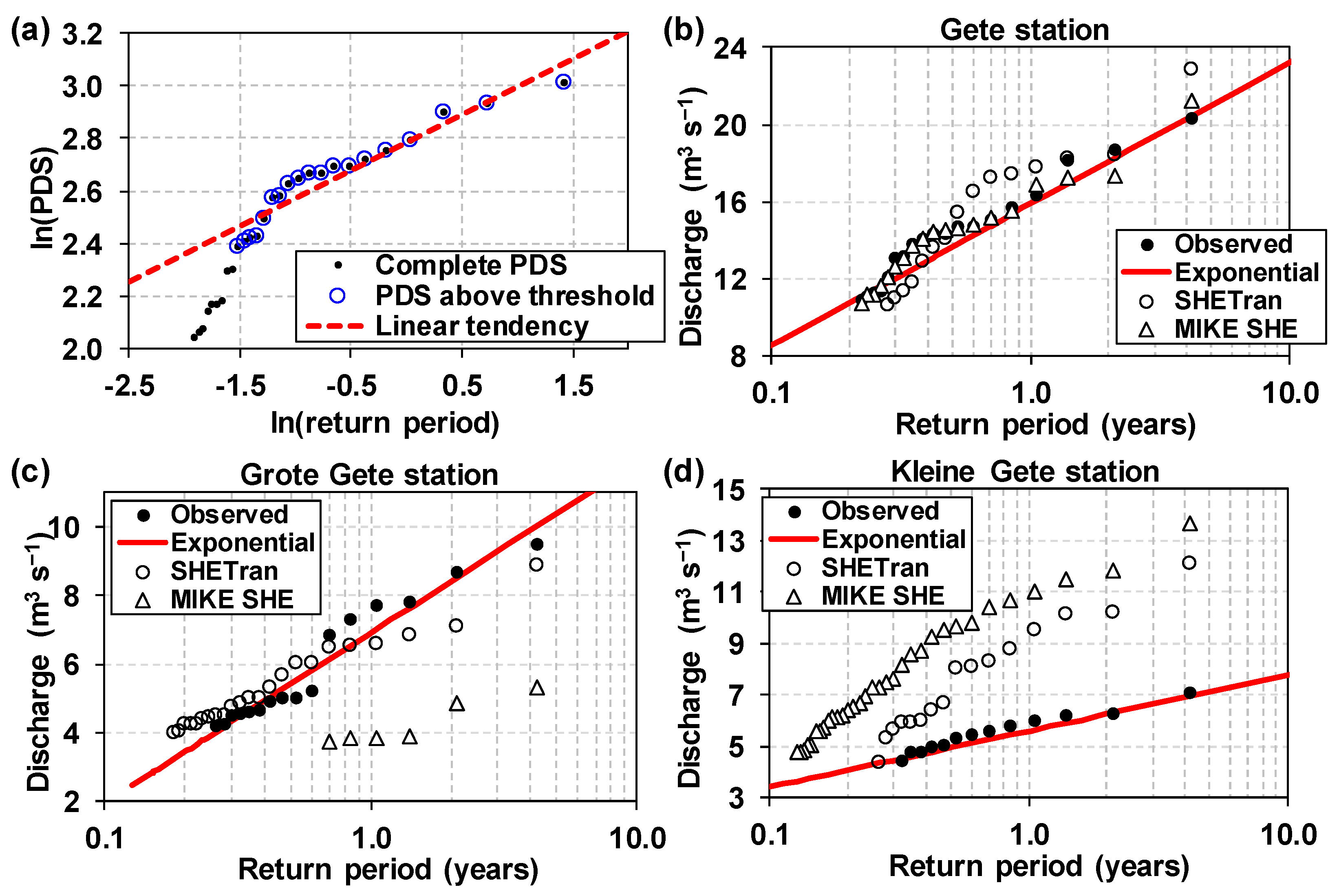
The analysis of the simulated time series considers whether it reproduces the peak flows, low flows and the hydrograph shape. For peak flows, daily values were used in the context of the peaks over threshold (POT) approach [57,58]. It considers the tail of a Generalised Pareto Distribution (GPD) that arises as the limiting distribution of peaks represented by a random variable x over a high threshold xth (i.e., x − xth). The GPD is shown in Equation (3) [57,59], where κsh and κsc are respectively the shape and scale parameters of the distribution:
In the case κsh = 0, G(x) is the exponential distribution. Weibull [9,37,57,60] plotting position of a quantile (observed extremes) was used for calculating the empirical probabilities of exceedance (and the respective empirical return periods). The daily peaks were selected from the total discharge series through a partial duration time series (PDS) approach [11,61,62]. Further information on the above methods can be found in Vázquez, Willems and Feyen [28].
For low flows, the baseflow (Qbs) component of the total hydrograph was used. This considers whether both the shape and magnitude of low flows were acceptably reproduced by the SHETRAN model. Qbs was estimated from the hydrograph for both the observed as well as the simulated hydrographs. This was achieved using a recursive digital filtering approach [63,64,65]. The approach assumes that Qbs, at every time step, evolves proportionally to Q, as given by the general expression used in signal analysis and processing [28]:
where Q(t) = total hydrograph (total signal) ordinate observed at time t [L3 T−1]; Fh(t) = high frequency filtering signal (quicker than the flow-component to be filtered) at time t [L3 T−1]; bF = proportionality factor [-]; aF and cF = filter coefficients [-]. aF may adopt a value between 0 and 1 (and may be thought of as the recession coefficient); the closer its value is to 1, the flatter the flow-component becomes. On the other hand, bF = (1 + aF)/2, whilst, cF = 1.0. The diverse variations of the high frequency filter used in this study (for instance, Vázquez [9],Nathan and McMahon [63], Arnold, Allen, Muttiah and Bernhardt [64], Chapman [66], Willems [67]) differ mainly on the values adopted by these three coefficients aF, bF and cF in response to the physical reasoning behind the formulation.
The low frequency filtered signal, Fl(t), is obtained at time t after subtracting the filtering signal, Fh(t), from the total flow, that is Fl(t) = Qbs = Q(t) − Fh(t). Further details can be found in Vázquez [9]. The filter is passed over the data several times in the forward and backward senses; commonly, three passes (forward, backward and forward again) are implemented with the intention of providing to the user some flexibility to adjust the baseflow estimation product more accurately to site-specific conditions.
3. Results
3.1. Values of the Effective Model Parameters
Table 2 lists the effective values of the parameters that were tuned during model calibration. With regard to the Manning roughness, for keeping the table to a reasonable size, only one value, for the fields cropped with maize, is listed for nov. With the same purpose in mind, only one value for nriv, the average for the whole river network, is listed. Further, the table includes the values of the hydrogeological parameters, calibrated for the geological formations that are in direct contact with the river network, considering two main subcatchments (i.e., zones “A” and “B”) defined by the water divide between the two main river branches of the study site (Figure 3a). For the other geological formations, the average parameter value for the whole catchment area is provided. The table shows that for some of the parameters the calibrated values obtained for both models are very similar in terms of magnitude; for the majority of the parameters, however, the respective calibrated values are importantly different in the two hydrological models.
3.2. Multi-Objective Model Performance Statistics
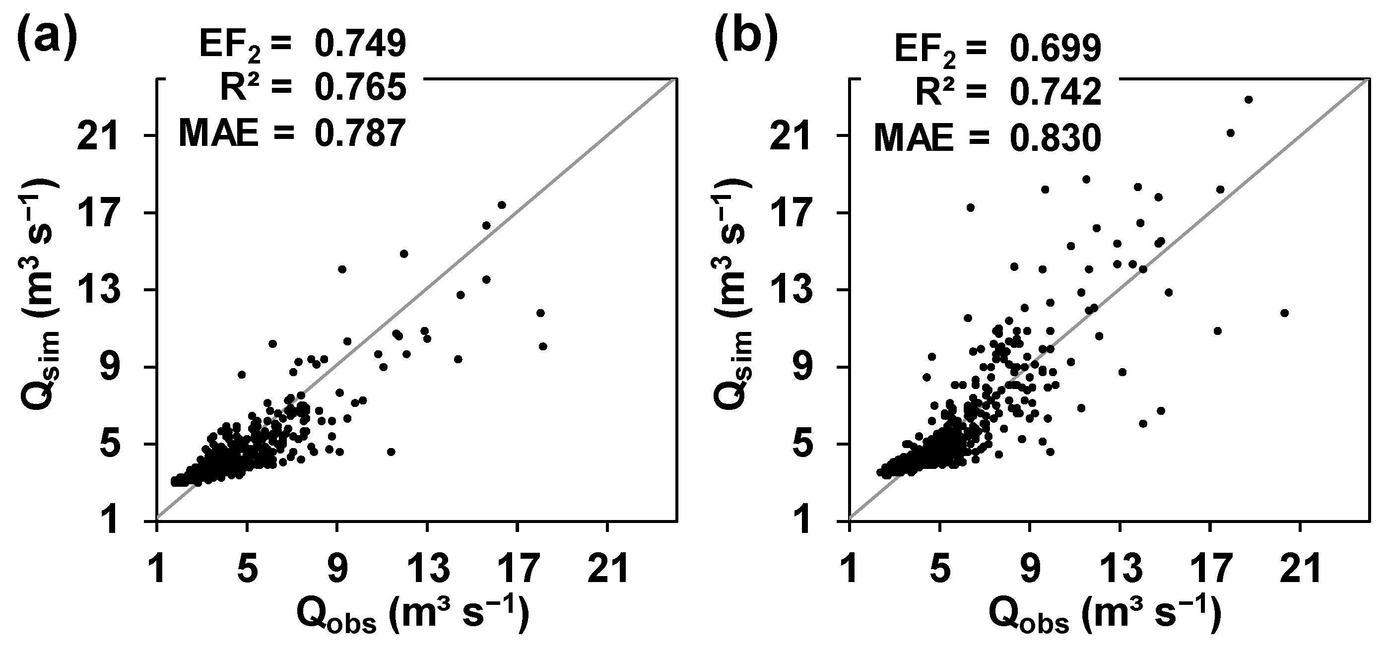
Peak flows were better predicted at the outlet of the catchment by SHETRAN in the calibration period than in the validation one (Figure 4), which is reflected by the better values of the model performance indices for the calibration period. Indeed, Figure 4b (validation period) depicts a wider dispersion of medium and peak flows, which produces the lower model performance. Obtaining better model performances for the calibration period is normal in hydrological modelling.
In general, low flows were over predicted by SHETRAN in both simulation periods. As expected, this was not properly identified by the performance indices (Figure 4), as these statistics used are known to be oversensitive to the simulation of peak flows [3,28,55] but far less sensitive to the simulation of low flows. Low flows simulation is considered in more detail in Section 3.4.
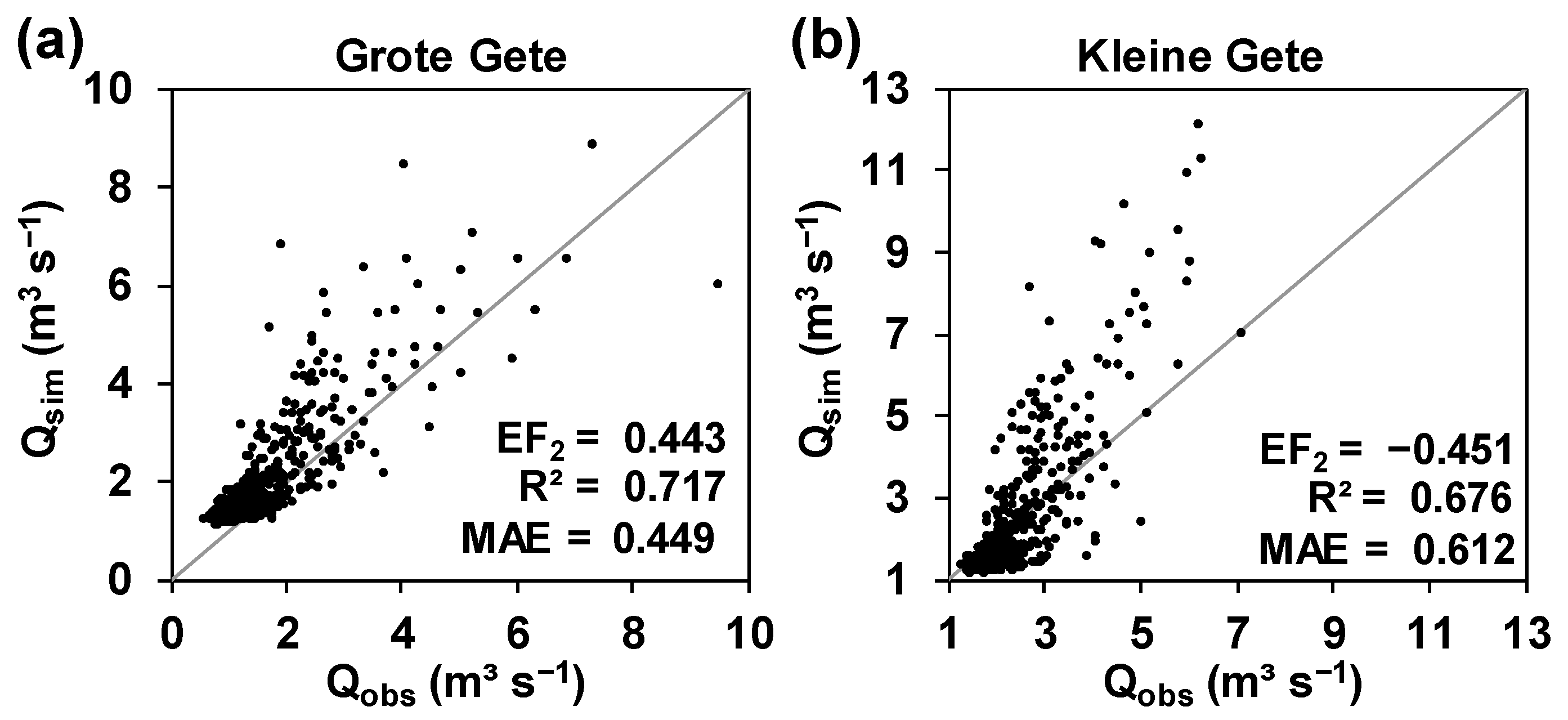
The MS model validation test (Figure 5) for the two internal stations show that the prediction of streamflow at locations that were not considered during model calibration was not as satisfactory as for the outlet of the catchment. This is emphasised by the values of the model performance indices, particularly by EF2. Indeed, this index shows that the predictions were worse for the Kleine Gete station, for which a negative EF2 value was obtained (Figure 5a). In general, streamflow predictions were better at the Grote Gete station (Figure 3d), although many lower, medium and peak flows were over predicted by the model (Figure 5b).
3.3. Comparison of the SHETRAN and MIKE SHE Predictions
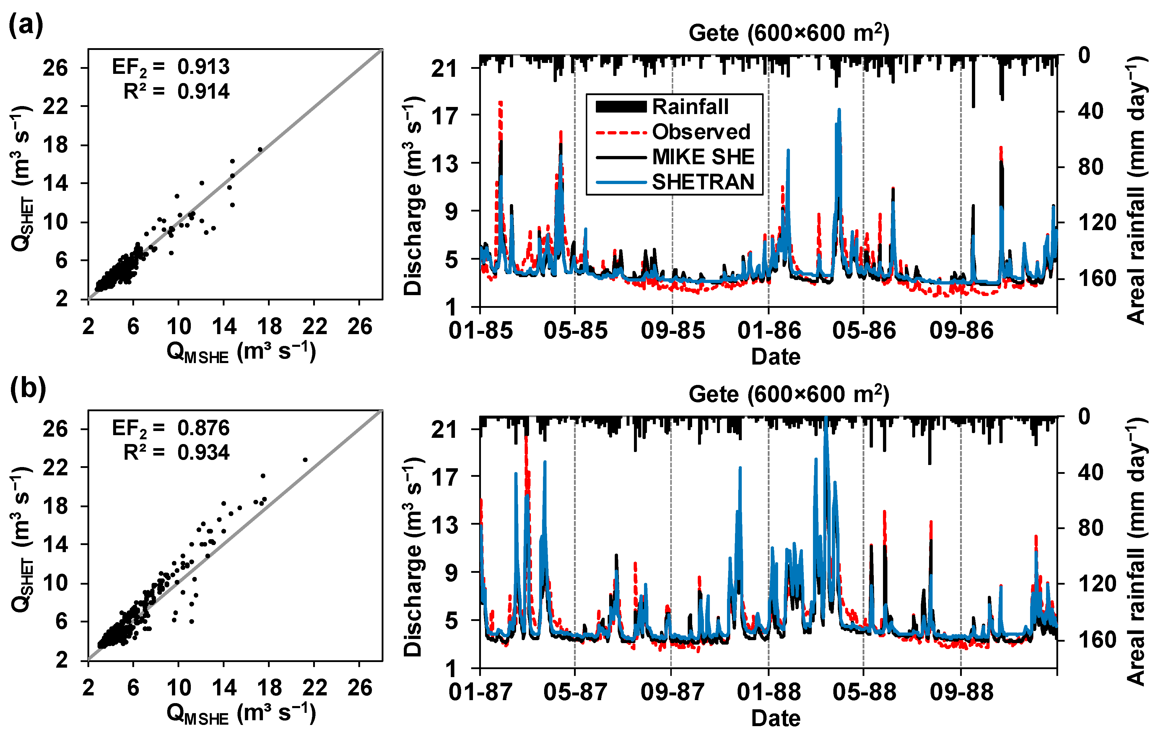
Comparison of the streamflow predictions at the outlet of the catchment for the calibration (Figure 6a) and validation (Figure 6b) periods show similar discharges for SHETRAN (QSHET) and MIKE SHE (QMSHE). This is emphasised by Figure 7, which shows that both SHETRAN (Figure 7a) and MIKE SHE (Figure 7b) had problems simulating streamflow at the outlet of the catchment in terms of peaks and low flows, which can also be seen in the performance statistics. Overall, peak flows were slightly better simulated by MIKE SHE (EF2 = 0.74; Figure 7b) than by SHETRAN (EF2 = 0.70; Figure 7a).
Figure 8 depicts the observed and simulated piezometric levels for some selected wells included in the analysis throughout the calibration and validation periods. The figure shows that the agreement between the observed and simulated piezometric levels, varied markedly, depending on the location within the catchment and the model. In some locations, SHETRAN had problems correctly simulating not only the main magnitude (with a maximum discrepancy of about 3.5 m, Figure 8a) but also the time evolution of piezometric levels (Figure 8a–c); although, in other locations, it represented acceptably well the observed piezometric- -magnitude and -evolution (Figure 8d). Whereas, MIKE SHE predicted the piezometric levels acceptably well in Figure 8a,b, but poorly in Figure 8c,d, where there was no variability in time.
3.4. Analysis of Simulated Time Series
Exponential distributions were obtained for the observed peaks in the calibration and validation periods for the three discharge stations (Figure 9). The POT method (Figure 9a), using the PDS of peak flows extracted automatically from the observed daily hydrographs, suggested peak thresholds (i.e., xth) of 10.9 m3 s−1 (Gete station), 3.9 m3 s−1 (Grote Gete station) and 4.4 m3 s−1 (Kleine Gete station), with which the empirical peak flow distributions of the simulated hydrographs were defined. With respect to the outlet of the study catchment at Gete station, peak flows were better simulated by MIKE SHE (Figure 9b); SHETRAN tended to over-predict them with a higher tendency than MIKE SHE. Moreover, both models had problems producing good predictions for the river discharge in the two internal stations, Grote Gete and Kleine Gete (Figure 9c,d) that were not part of the model calibration (i.e., MS test). However, the SHETRAN results were better than those from MIKE SHE, particularly at Grote Gete.
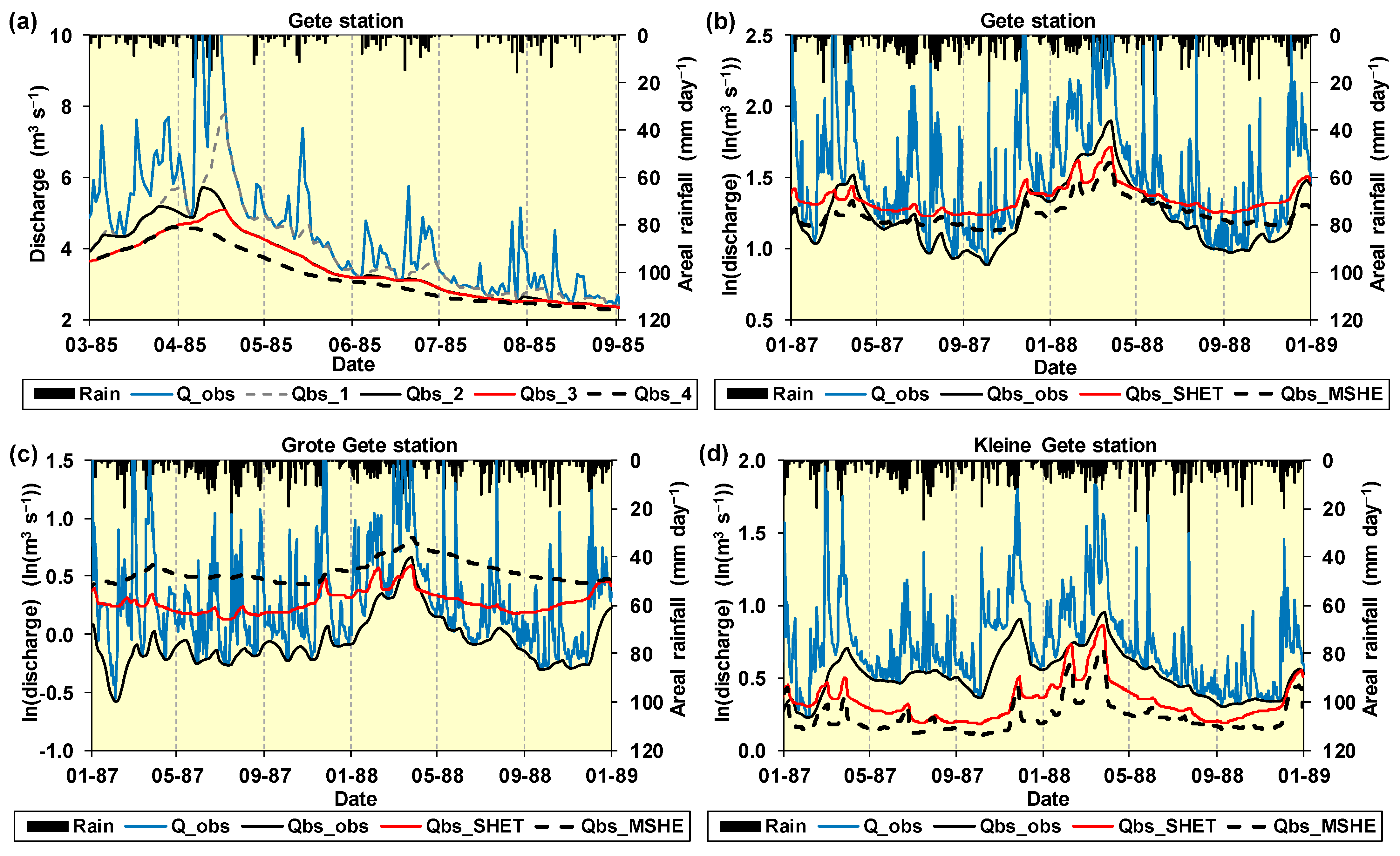
Figure 10a illustrates the outcome for estimating the Qbs time series for the Gete station. Four series corresponding to four (forward and backward) passes of the filter are plotted in the figure. Flatter series were obtained for the higher passes. Additionally, the higher the value adopted by the aF coefficient, the flatter the Qbs series became. A value of 0.94 for aF and the third pass of the filter applied on the observed streamflow were used after comparison with the estimates produced by a previous work that used a more sophisticated recursive filter [9]. This aF value and the third pass were also used for filtering the simulated streamflow from SHETRAN and MIKE SHE.
The magnitudes of the Qbs series obtained for the simulated hydrographs are, in general, higher than the respective magnitudes of the series derived from the observed streamflow in the Gete station, particularly in the periods May-December in 1987 and 1988 (Figure 10b). This accentuates what was already observed in Figure 4: an over-prediction of low flows for both the calibration and validation periods for the SHETRAN model. Qbs estimates were higher for the model predictions than for the observations in the case of the Grote Gete station (Figure 10c). Whereas for the Kleine Gete station (Figure 10d), an under-prediction of the baseflow was observed.
In general, and although not depicted in this manuscript, the frequency analysis of annual historical discharge for the Gete station in the period 1984–1996 showed that the average base flow (Qbs) fraction was 69.2%. This shows the dominant contribution of Qbs to the overall discharge, and is in agreement with the importance of aquifers not only in Flanders, the northern region of Belgium, but also throughout Belgium [68].
4. Discussion
The aim of this research considered the evaluation of the capabilities of SHETRAN for working with geologically complex systems. This is the first attempt to apply SHETRAN on such geologically complex non-experimental study sites. In addition, robust model evaluation was carried out using a multi-objective (using uncorrelated error measures) and MS evaluation protocol on the SHETRAN predictions, which is an aspect that conventionally has not been fully explored. Of the existing research that does consider multi-objective functions (e.g., Zhang, Moreira and Corte-Real [6], Op de Hipt, Diekkrüger, Steup, Yira, Hoffmann and Rode [25], Op de Hipt, Diekkrüger, Steup, Yira, Hoffmann and Rode [26] and Op de Hipt, Diekkrüger, Steup, Yira, Hoffmann, Rode and Näschen [15]) they often use performance measures that are either correlated or measuring the same type of modelling error or performance measures that are oversensitive to peak simulations. Further, the MS evaluation is more in line with the distributed nature of PBD codes than the simple SS test. Indeed, in the current modelling exercise, it revealed important simulation pitfalls for the internal river discharge and piezometric stations/wells. This MS test is therefore very useful in addressing data uncertainties (and locations within the catchment where additional data gathering efforts have to be carried out in the future) and also unsuitable modelling approaches/scales, etc. The issues with simulating the piezometric stations/wells also highlights (i) the mismatch between the 600 × 600 m2 modelling scale and the point scale at which observations were collected; and (ii) the significant load of uncertainty attached to some of the geological data used to build the geological model of the study catchment.
When looking at the comparison between SHETRAN and MIKE SHE based models there are two aspects to consider. Firstly, the ease of setting up the models and the evaluation of the output data and, secondly, the difference in the model structure and coding. With regards to setting up the models the vertical discretisation of the soil and geological components is easy in MIKE SHE. In SHETRAN its implementation is more complex. Indeed, setting up the hydrological model of the geologically complex study site using the free-license set of data processing software tools accompanying the SHETRAN code was not a straight task in this study, with specific-task subroutines needing to be developed to overcome the shortage of user-friendly SHETRAN software tools for the pre-processing of input data when simulating geologically complex catchments. Once these tools had been developed, all the geometrical characteristics of the surface, subsurface and deep underground components of the catchment could be successfully included in the model. But working with the respective software tools available as a part of the commercial-license MIKE SHE code was markedly easier. Similarly, most of the tasks included in model evaluation were easier with the aid of the data processing tools accompanying the MIKE SHE code than it was with the respective free-license SHETRAN code tools; although in both cases it required to a certain extent the building of specific-tasks subroutines.
Considering the model structure and coding, the main difference between the codes that were used in this research is the subsurface component. While SHETRAN uses a 3-dimensional (3D) variably saturated subsurface flow model, MIKE SHE uses a simplified 1-dimensional UZ modelling approach and a 2D or 3D SZ modelling approach (Figure 2). This structural discrepancy is likely to affect the simulation of infiltration and recharge to deeper aquifers. It will therefore affect the different piezometric predictions produced by the two models. Although some discrepancies in the semiautomatic processes for model construction, calibration and validation might have also contributed to them. Another aspect that may have contributed to obtain not only different piezometric predictions but also surface flow predictions is the different ETact approaches in SHETRAN and MIKE SHE. There are other related issues that are different between the codes which are more related to data format, etc. Hence, in the MIKE SHE code there is a clear differentiation between “soils” (UZ) and the underlying geological units (SZ), not only in terms of the different physical and hydraulic parameters, but also, geometrically and functionally (i.e., water table fluctuates only in the SZ, implying a readjustment of the uppermost limit of the SZ). In SHETRAN, this differentiation is less clear, at least in terms of the definition of the physical parameters. For instance, in MIKE SHE, the specific storage is exclusively a hydrogeological parameter, whilst in SHETRAN it is also stored in the soils database. Further, in MIKE SHE both, the specific yield (Sy) and the specific storage (Ss) need to be specified for, respectively, unconfined and confined aquifers, which is not the case for SHETRAN where only a single storage value needs to be specified (and the code decides how to use it under, either, unconfined or confined conditions).
The used MIKE SHE version includes one of the last Unix® (Linux®) based graphical user interface (GUI) versions that were commercially “adapted” to work in Windows®. Before focusing entirely on a 100% Windows® based GUI, the producer of the code (Danish Hydraulic Institute, DHI) incorporated in this version 2001 a second option for (1D) river modelling, which was DHI code MIKE 11 [69]. Starting from the fully Windows® based version in 2002 this became its only river modelling module until very recently, when they added as a newer option their code MIKE HYDRO River [70]. Although it was never the aim of this study to assess the effects of these MIKE SHE code structural changes, because we were always focused on the performance of SHETRAN, we are in a position to state that, despite these structural changes, the respective MIKE SHE based model predictions of the discharge at the outlet of the study site (using MIKE 11) are similar to the ones reported herein. Further, the newest versions of MIKE SHE still use a simplified 1D UZ modelling approach, implying that this part of its structure has not (yet) been modified.
It is believed that further work should focus on improving the availability of pre-processing and post-processing software tools accompanying the SHETRAN code, for both preparing input files (or importing ASCII data, including maps) to easily set-up a model of any geologically complex hydrological system, and easily exporting model outputs to a diverse set of ASCII formats (i.e., space delimited, comma delimited, matrix data, etc.). These would facilitate both model reporting and either automatic calibration or Monte Carlo based sensitivity analyses. It would definitively enhance not only the practical use of this free-license powerful distributed model but also the possibility of easily incorporating into the modelling either remote sensing or other sources of distributed information. Hence, although for computational optimisation binary formats should be preferred, the implementation of software tools for easily handling ASCII formats should be potentiated rather than demonised so that average-skilled practitioners and scientists could get the most out of SHETRAN by easily defining input files (and importing from diverse graphical software) using ASCII formats, and so make the code more accessible.
Although it was never the aim of this research to evaluate the SHETRAN structure nor suggest any modification of it, it is believed that future work should also focus on enhancing the capabilities of SHETRAN, say, for implementing the possibility of carrying out not only rainfall-runoff simulation but also rainfall-stage modelling. This enhancement would provide SHETRAN with the important capability of reducing significant data uncertainty that is normally attached to river discharges derived from rating curves [13].
Finally, the main message of this paper is that the use of the free-license code SHETRAN in any real case or research applications is as feasible as using any similar commercial-license model. There is not any modelling constraint besides the additional programming of specific-task subroutines or the manual completion of needed modelling tasks. In this context, modellers could benefit from the high potentials that the structure of SHETRAN offers for the integrated (simultaneous surface, subsurface and groundwater) modelling of hydrological systems.
5. Conclusions
There is a demand for modelling hydrological complex catchments using cheap and reliable mechanistic codes. This work has tested a code of this type, the free-license PBD SHETRAN code, on a geologically complex 586 km2 catchment. The complex geometry of the study catchment that included six geological units, as well as the spatial variability of the different physical parameters, was successfully incorporated into the distributed model of the site. The model was calibrated by tuning the values of the Manning’s roughness parameters for the simulation of overland flow and river discharge, as well as, the hydraulic conductivities of the geological units. In general, the discharge simulation at the catchment outlet was acceptable, although some peak and low flows were not well simulated. Discharge predictions were of inferior quality for the two internal stations that were not considered in model calibration. The quality of the piezometric predictions varied, mainly as a function of the location of a given piezometric well in the catchment and of the geological unit where its screen was located. Overall, the discharge and piezometric predictions of SHETRAN and the similar but commercial-license MIKE SHE code were comparable. Further, all the modelling approaches and tests that could be implemented with the MIKE SHE code could be also implemented with SHETRAN, although SHETRAN needed the programming of a larger number of specific-task subroutines for data handling. All this encourages the use of the free-license SHETRAN code for carrying out the distributed modelling of geologically complex systems.
Author Contributions
Conceptualisation, R.F.V., J.E.B. and H.H.; methodology, R.F.V., J.E.B. and S.B.; validation, J.E.B., R.F.V. and S.B.; formal analysis, J.E.B. and R.F.V.; investigation, J.E.B., R.F.V., H.H. and S.B.; resources, R.F.V. and H.H.; writing—original draft preparation, R.F.V., J.E.B. and H.H.; writing—review and editing, R.F.V., J.E.B., H.H. and S.B.; visualization, R.F.V. and H.H.; supervision, R.F.V. and H.H.; project administration, R.F.V. and H.H.; funding acquisition, R.F.V. and H.H. All authors have read and agreed to the published version of the manuscript.
Funding
This research received no external funding. The APC was kindly funded by the University of Cuenca, Ecuador.
Data Availability Statement
Restrictions apply to the availability of data used in this research. Data was obtained from several public Belgian institutions and might be available directly from them. These institutions include: the Department Water of AMINAL, DIHO; OC GIS-Vlaanderen; the Royal Meteorological Institute of Belgium; the Flemish Community Department Afdeling Natuurlijke Rijkdommen en Energie; the Laboratory of Hydrogeology and the former Institute of Soil and Water Management of the KULeuven; the Belgian Geological Survey; Le Ministère de la Region Wallone, Direction Générale des Resources Naturelles et de l’Environment, Division d’Eau, Service des Eaux Souterraines and the Centre d’Environment, Université de Liège.
Acknowledgments
Part of the modelling experiments reported herein took place in the scope of the project “Water Management and Climate Change in the Focus of International Master Courses (WATERMAS)” financed by the European “Education, Audiovisual and Culture Executive Agency (EACA)” and directed locally by the first author. Also, in the scope of this project, the second author benefitted from a research stay at the University of Ghent, Belgium. This publication reflects only the authors’ views; thereby, neither the European Union nor EACA is liable for any use that may be made of the information contained herein.
Conflicts of Interest
The authors declare no conflict of interest. The funders had no role in the design of the study; in the collection, analyses, or interpretation of data; in the writing of the manuscript; or in the decision to publish the results.
References
- Feyen, J.; Vázquez, R.F. Modeling hydrological consequences of climate and land use change—Progress and Challenges. MASKANA 2011, 2, 83–100. [Google Scholar] [CrossRef]
- Refsgaard, J.C. Parameterisation, calibration and validation of distributed hydrological models. J. Hydrol. 1997, 198, 69–97. [Google Scholar] [CrossRef]
- Vázquez, R.F.; Feyen, L.; Feyen, J.; Refsgaard, J.C. Effect of grid-size on effective parameters and model performance of the MIKE SHE code applied to a medium sized catchment. Hydrol. Process. 2002, 16, 355–372. [Google Scholar] [CrossRef]
- Beven, K.J. Rainfall-Runoff Modelling: The Primer, 2nd ed.; John Wiley and Sons: Chichester, UK, 2012; p. 457. [Google Scholar]
- Zhang, R.; Santos, C.A.G.; Moreira, M.; Freire, P.K.M.M.; Corte-Real, J. Automatic Calibration of the SHETRAN Hydrological Modelling System Using MSCE. Water Resour. Manag. 2013, 27, 4053–4068. [Google Scholar] [CrossRef] [Green Version]
- Zhang, R.; Moreira, M.; Corte-Real, J. Multi-objective calibration of the physically based, spatially distributed SHETRAN hydrological model. J. Hydroinformatics 2016, 18, 428–445. [Google Scholar] [CrossRef] [Green Version]
- Zhang, J.; Zhang, M.; Song, Y.; Lai, Y. Hydrological simulation of the Jialing River Basin using the MIKE SHE model in changing climate. J. Water Clim. Change 2021, 12, 2495–2514. [Google Scholar] [CrossRef]
- Madsen, H. Parameter estimation in distributed hydrological catchment modelling using automatic calibration with multiple objectives. Adv. Water Resour. 2003, 26, 205–216. [Google Scholar] [CrossRef]
- Vázquez, R.F. Assessment of the performance of physically based distributed codes simulating medium size hydrological systems. Doctoral Dissertation, Katholieke Universiteit Leuven (K.U. Leuven), Leuven, Belgium, 2003. [Google Scholar]
- McMichael, C.E.; Hope, A.S.; Loaiciga, H.A. Distributed hydrological modelling in California semi-arid shrublands: MIKE SHE model calibration and uncertainty estimation. J. Hydrol. 2006, 317, 307–324. [Google Scholar] [CrossRef]
- Vázquez, R.F.; Beven, K.; Feyen, J. GLUE based assessment on the overall predictions of a MIKE SHE application. Water Resour. Manag. 2009, 23, 1325–1349. [Google Scholar] [CrossRef]
- Vázquez, R.F.; Hampel, H. Prediction limits of a catchment hydrological model using different estimates of ETp. J. Hydrol. 2014, 513, 216–228. [Google Scholar] [CrossRef]
- Vázquez, R.F.; Hampel, H. A Simple Approach to Account for Stage-Discharge Uncertainty in Hydrological Modelling. Water 2022, 14, 1045. [Google Scholar] [CrossRef]
- Guerreiro, S.B.; Birkinshaw, S.; Kilsby, C.; Fowler, H.J.; Lewis, E. Dry getting drier—The future of transnational river basins in Iberia. J. Hydrol. Reg. Stud. 2017, 12, 238–252. [Google Scholar] [CrossRef]
- Op de Hipt, F.; Diekkrüger, B.; Steup, G.; Yira, Y.; Hoffmann, T.; Rode, M.; Näschen, K. Modeling the effect of land use and climate change on water resources and soil erosion in a tropical West African catch-ment (Dano, Burkina Faso) using SHETRAN. Sci. Total Environ. 2019, 653, 431–445. [Google Scholar] [CrossRef] [PubMed]
- Cieśliński, R. Determination of retention value using Mike She model in the area of young glacial catchments. Appl. Water Sci. 2020, 11, 5. [Google Scholar] [CrossRef]
- Ewen, J.; Parkin, G.; O’Connell Patrick, E. SHETRAN: Distributed River Basin Flow and Transport Modeling System. J. Hydrol. Eng. 2000, 5, 250–258. [Google Scholar] [CrossRef] [Green Version]
- Mourato, S.; Moreira, M.; Corte-Real, J. Water Resources Impact Assessment under Climate Change Scenarios in Mediterranean Watersheds. Water Resour. Manag. 2015, 29, 2377–2391. [Google Scholar] [CrossRef]
- Đukić, V.; Radić, Z. Sensitivity Analysis of a Physically based Distributed Model. Water Resour. Manag. 2016, 30, 1669–1684. [Google Scholar] [CrossRef]
- Shrestha, P.K.; Shakya, N.M.; Pandey, V.P.; Birkinshaw, S.J.; Shrestha, S. Model-based estimation of land subsidence in Kathmandu Valley, Nepal. Geomat. Nat. Hazards Risk 2017, 8, 974–996. [Google Scholar] [CrossRef] [Green Version]
- Sreedevi, S.; Eldho, T.I.; Madhusoodhanan, C.G.; Jayasankar, T. Multiobjective sensitivity analysis and model parameterization approach for coupled streamflow and groundwater table depth simulations using SHETRAN in a wet humid tropical catchment. J. Hydrol. 2019, 579, 124217. [Google Scholar] [CrossRef]
- Suroso; Wahyuni, A.D.; Santoso, P.B. Prediction of Streamflow at the Pemali catchment area using Shetran model. IOP Conf. Ser. Earth Environ. Sci. 2021, 698, 012009. [Google Scholar] [CrossRef]
- Birkinshaw, S.J.; O’Donnell, G.; Glenis, V.; Kilsby, C. Improved hydrological modelling of urban catchments using runoff coefficients. J. Hydrol. 2021, 594, 125884. [Google Scholar] [CrossRef]
- Escobar-Ruiz, V.; Smith, H.G.; Blake, W.H.; Macdonald, N. Assessing the performance of a physically based hydrological model using a proxy-catchment approach in an agricultural environment. Hydrol. Processes 2019, 33, 3119–3137. [Google Scholar] [CrossRef] [Green Version]
- Op de Hipt, F.; Diekkrüger, B.; Steup, G.; Yira, Y.; Hoffmann, T.; Rode, M. Applying SHETRAN in a Tropical West African Catchment (Dano, Burkina Faso)—Calibration, Validation, Uncertainty Assessment. Water 2017, 9, 101. [Google Scholar] [CrossRef] [Green Version]
- Op de Hipt, F.; Diekkrüger, B.; Steup, G.; Yira, Y.; Hoffmann, T.; Rode, M. Modeling the impact of climate change on water resources and soil erosion in a tropical catchment in Burkina Faso, West Africa. CATENA 2018, 163, 63–77. [Google Scholar] [CrossRef]
- Thiemann, M.; Trosser, M.; Gupta, H.; Sorooshian, S. Bayesian recursive parameter estimation for hydrologic models. Water Resour. Res. 2001, 37, 2521–2536. [Google Scholar] [CrossRef]
- Vázquez, R.F.; Willems, P.; Feyen, J. Improving the predictions of a MIKE SHE catchment-scale application by using a multi-criteria approach. Hydrol. Process. 2008, 22, 2159–2179. [Google Scholar] [CrossRef]
- Feyen, L.; Vazquez, R.F.; Christiaens, K.; Sels, O.; Feyen, J. Application of a distributed physically-based hydrological model to a medium size catchment. Hydrol. Earth Syst. Sci. 2000, 4, 47–63. [Google Scholar] [CrossRef]
- Birkinshaw, S.J. Technical note: Automatic river network generation for a physically-based river catchment model. Hydrol. Earth Syst. Sci. 2010, 14, 1767–1771. [Google Scholar] [CrossRef] [Green Version]
- Refsgaard, J.C.; Storm, B. MIKE SHE. In Computer Models of Watershed Hydrology; Singh, V.P., Ed.; Water Resources Publications: Littleton, CO, USA, 1995; pp. 809–846. [Google Scholar]
- Ma, L.; He, C.; Bian, H.; Sheng, L. MIKE SHE modeling of ecohydrological processes: Merits, applications, and challenges. Ecol. Eng. 2016, 96, 137–149. [Google Scholar] [CrossRef]
- Abbott, M.B.; Bathurst, J.C.; Conge, P.E.; O’Connell, P.E.; Rasmussen, J. An introduction to the European Hydrological System Système Hydrologique Européen, ‘SHE’, 1. History and philosophy of a physically based distributed modeling system. J. Hydrol. 1986, 87, 45–59. [Google Scholar] [CrossRef]
- Abbott, M.B.; Bathurst, J.C.; Cunge, P.E.; O’Connell, P.E.; Rasmussen, J. An introduction to the European Hydrological System Systéme Hydrologique Européen, ‘SHE’, 2. Structure of a Physically-based, Distributed Modelling System. J. Hydrol. 1986, 87, 61–77. [Google Scholar] [CrossRef]
- Bathurst, J.C.; Birkinshaw, S.J.; Cisneros, F.; Fallas, J.; Iroumé, A.; Iturraspe, R.; Novillo, M.G.; Urciuolo, A.; Alvarado, A.; Coello, C.; et al. Forest impact on floods due to extreme rainfall and snowmelt in four Latin American environments 2: Model analysis. J. Hydrol. 2011, 400, 292–304. [Google Scholar] [CrossRef]
- Vázquez, R.F.; Feyen, J. Assessment of the performance of a distributed code in relation to the ETp estimates. Water Resour. Manag. 2002, 16, 329–350. [Google Scholar] [CrossRef]
- Vázquez, R.F.; Feyen, J. Assessment of the effects of DEM gridding on the predictions of basin runoff using MIKE SHE and a modelling resolution of 600 m. J. Hydrol. 2007, 334, 73–87. [Google Scholar] [CrossRef]
- Vereecken, H. Pedotransferfunctions for the generation of hydraulic properties for Belgian soils. Doctoral Dissertation, Katholieke Universiteit Leuven (K.U.Leuven), Leuven, Belgium, 1988. [Google Scholar]
- Allen, G.R.; Pereira, L.S.; Raes, D.; Martin, S. Crop Evapotranspiration-Guidelines for Computing Crop Water Requirements; FAO: Rome, Italy, 1998; p. 300. [Google Scholar]
- Vázquez, R.F.; Feyen, J. Potential Evapotranspiration for the distributed modelling of Belgian basins. J. Irrig. Drain. Eng. 2004, 130, 1–8. [Google Scholar] [CrossRef]
- Feddes, R.A.; Kowalik, P.; Neuman, S.P.; Bresler, E. Finite difference and finite element simulation of field water uptake by plants/Simulation de la différence finie et de l’élément fini de l’humidité du sol utilisée par les plantes. Hydrol. Sci. Bull. 1976, 21, 81–98. [Google Scholar] [CrossRef]
- Shuttleworth, W.J. Evaporation. In Handbook of Hydrology; Maidment, D.R., Ed.; McGRaw Hill: New York, NY, USA, 1993; Volume 1, pp. 4.1–4.47. [Google Scholar]
- NU. SHETRAN Water Flow Component, Equations and Algorithms; Newcastle University: Newcastle, UK, 2001; p. 55. [Google Scholar]
- Rutter, A.J.; Kershaw, K.A.; Robins, P.C.; Morton, A.J. A predictive model of rainfall interception in forests, 1. Derivation of the model from observations in a plantation of Corsican pine. Agric. Meteorol. 1971, 9, 367–384. [Google Scholar] [CrossRef]
- Boons-Prins, E.R.; Koning, G.H.J.D.; Diepen, C.A.V.; Penning, F.W.T.D. Crop-Specific Simulation Parameters for Yield Forecasting across the European Community; Centre for Agrobiological Research: Wageningen, The Netherlands, 1993; p. 200. [Google Scholar]
- Breuer, L.; Eckhardt, K.; Frede, H.-G. Plant parameter values for models in temperate climates. Ecol. Model. 2003, 169, 237–293. [Google Scholar] [CrossRef]
- Kristensen, K.J.; Jensen, S.E. A model for estimating actual evapotranspiration from potential evapotranspiration. Nord. Hydrol. 1975, 6, 170–188. [Google Scholar] [CrossRef] [Green Version]
- Engman, E.T. Roughness coefficients for routing surface runoff. J. Irrig. Drain. Eng. 1986, 112, 39–53. [Google Scholar] [CrossRef]
- Chow, V.T.; Maidment, D.R.; Mays, L.W. Applied Hydrology; McGraw-Hill International Editions: Singapore, 1988; p. 572. [Google Scholar]
- Anderson, M.P.; Woessner, W.W.; Hunt, R. Applied Groundwater Modelling Simulation of Flow and Advective Transport, 2nd ed.; Academic Press: Cambridge, MA, USA, 2015; p. 630. [Google Scholar]
- Dehotin, J.; Vázquez, R.F.; Braud, I.; Debionne, S.; Viallet, P. Hydrological modelling using unstructured and irregular grids: Example of 2D groundwater modelling. J. Hydrol. Eng. 2011, 16, 108–125. [Google Scholar] [CrossRef] [Green Version]
- Biondi, D.; Freni, G.; Iacobellis, V.; Mascaro, G.; Montanari, A. Validation of hydrological models: Conceptual basis, methodological approaches and a proposal for a code of practice. Phys. Chem. Earth Parts A/B/C 2012, 42–44, 70–76. [Google Scholar] [CrossRef]
- Li, D.; Liang, Z.; Zhou, Y.; Li, B.; Fu, Y. Multicriteria assessment framework of flood events simulated with vertically mixed runoff model in semiarid catchments in the middle Yellow River. Nat. Hazards Earth Syst. Sci. 2019, 19, 2027–2037. [Google Scholar] [CrossRef] [Green Version]
- Bizhanimanzar, M.; Leconte, R.; Nuth, M. Modelling of shallow water table dynamics using conceptual and physically based integrated surface-water–groundwater hydrologic models. Hydrol. Earth Syst. Sci. 2019, 23, 2245–2260. [Google Scholar] [CrossRef] [Green Version]
- Legates, D.R.; McCabe, G.J. Evaluating the use of ‘goodness-of-fit’ measures in hydrological and hydroclimatic model validation. Water Resour. Res. 1999, 35, 233–241. [Google Scholar] [CrossRef]
- Nash, J.E.; Sutcliffe, J. River flow forecasting through conceptual models, I, A discussion of principles. J. Hydrol. 1970, 10, 282–290. [Google Scholar] [CrossRef]
- Willems, P. Compound intensity/duration/frequency-relationships of extreme precipitation for two seasons and two storm types. J. Hydrol. 2000, 233, 189–205. [Google Scholar] [CrossRef]
- Pandey, M.D.; van Gelder, P.H.A.J.M.; Vrijling, J.K. Bootstrap simulations for evaluating the uncertainty associated with peaks-over-threshold estimates of extreme wind velocity. Environmetrics 2003, 14, 27–43. [Google Scholar] [CrossRef]
- Pickands, J. Statistical Inference using extreme order statistics. Annals Stat. 1975, 3, 119–131. [Google Scholar]
- Hong, H.P.; Li, S.H. Plotting positions and approximating first two moments of order statistics for Gumbel distribution: Estimating quantiles of wind speed. Wind. Struct. 2014, 19, 371–387. [Google Scholar] [CrossRef]
- Stedinger, J.R.; Vogel, R.M.; Foufoula-Georgiou, E.F. Frequency Analysis of extreme events. In Handbook of Hydrology; Maidment, D.R., Ed.; McGraw-Hill Inc.: New York, NY, USA, 1993; pp. 18.11–18.66. [Google Scholar]
- Vimos-Lojano, D.J.; Martínez-Capel, F.; Hampel, H.; Vázquez, R.F. Hydrological influences on aquatic communities at the mesohabitat scale in high Andean streams of southern Ecuador. Ecohydrology 2019, 12, e2033. [Google Scholar] [CrossRef]
- Nathan, R.J.; McMahon, T.A. Evaluation of automated techniques for baseflow and recession analysis. Water Resour. Res. 1990, 26, 1465–1473. [Google Scholar] [CrossRef]
- Arnold, J.G.; Allen, P.M.; Muttiah, R.; Bernhardt, G. Automated Base Flow Separation and Recession Analysis Techniques. Groundwater 1995, 33, 1010–1018. [Google Scholar] [CrossRef]
- Ahiablame, L.; Chaubey, I.; Engel, B.; Cherkauer, K.; Merwade, V. Estimation of annual baseflow at ungauged sites in Indiana USA. J. Hydrol. 2013, 476, 13–27. [Google Scholar] [CrossRef]
- Chapman, T. Comment on “Evaluation of automated techniques for base flow and recession analyses” by R. J. Nathan and T. A. McMahon. Water Resour. Res. 1991, 27, 1783–1784. [Google Scholar] [CrossRef]
- Willems, P. A time series tool to support the multi-criteria performance evaluation of rainfall-runoff models. Environ. Model. Softw. 2009, 24, 311–321. [Google Scholar] [CrossRef]
- Houthuys, R. A sedimentary model of the Brussels Sands, Eocene, Belgium. Geol. Belg. 2011, 14, 55–74. [Google Scholar]
- DHI. MIKE-SHE v 2001 User Guide and Technical Reference Manual; Danish Hydraulic Institute: Horsolm, Denmark, 2001. [Google Scholar]
- DHI. MIKE SHE User Guide and Reference Manual; Danish Hydraulic Institute: Horsolm, Denmark, 2022; p. 820. [Google Scholar]
Figure 1.
(a) Location of the study site, the Gete catchment (after Vázquez, Willems and Feyen [28]); (b) digital terrain model (DTM) of the study site and horizontal distribution of (c) the vertical profiles of the simplified geological model of the study site (600 × 600 m2) showing the thin loamy Quarternarian deposits (Kw) overlaying the dipping formations, sandy Brusseliaan (Br), clayey sand Landeniaan (Ln), sandy very fine marls Heers (Hr), white chalk Cretaceous (Cr). Below these layers is the Palaeozoic strongly folded rocky basement.

Figure 3.
600 × 600 m2 model river networks for (a) SHETRAN and (b) MIKE SHE; (c) distribution of rainfall stations used in the modelling and associated Thiessen polygons (after Vázquez [9]); and (d) location of the calibration and evaluation stream gauging stations and observation wells (after Vázquez [9]). Topographical colour scales are different in (a,b) owing to the use of different software tools (accompanying the SHETRAN and MIKE SHE codes) to create the plots. Plot (a) shows the water divide (white dashed line) that determines subcatchments (zones) A and B that were considered for the spatial calibration of some hydrogeological parameters. MS = multi-site model performance validation test; SS = split-sample model performance validation test. Coordinates system: Lambert conformal conic for Belgium.

Figure 4.
Scatter plots of total streamflow observed (Qobs) and predicted (Qsim) by SHETRAN, at the outlet of the catchment, for (a) the calibration period [1 of January 1985–31 of December 1986]; and (b) the validation period [1 of January 1987–31 of December 1988]. EF2 = Coefficient of Efficiency (Nash and Sutcliffe Efficiency); R2 = square of the Pearson’s type (linear) correlation coefficient; MAE = Mean Absolute Error.

Figure 5.
Multi-site (MS) scatter plots for the validation period [1 January 1987–31 December 1988] of observed (Qobs) and SHETRAN predicted (Qsim) total streamflow at the non-calibrated stations (a) Grote Gete; and (b) Kleine Gete (Figure 3d). EF2 = Coefficient of Efficiency (Nash and Sutcliffe Efficiency); R2 = square of the Pearson’s type (linear) correlation coefficient; MAE = Mean Absolute Error.

Figure 6.
Scatter plots and hydrographs of MIKE SHE (QMSHE) and SHETRAN (QSHET) total streamflow simulations at the outlet of the catchment for (a) the calibration period [1 January 1985–31 December 1986]; and (b) the validation period [1 January 1987–31 December 1988]. EF2 = Coefficient of Efficiency (Nash and Sutcliffe Efficiency); R2 = square of the Pearson’s type (linear) correlation coefficient.

Figure 7.
Scatter plots and hydrographs of total streamflow observed (Qobs) and predicted (Qsim) at the outlet of the catchment, for the validation period. Predictions were produced by (a) SHETRAN; and (b) MIKE SHE. EF2 = Coefficient of Efficiency (Nash and Sutcliffe Efficiency); R2 = square of the Pearson’s type (linear) correlation coefficient; MAE = Mean Absolute Error.

Figure 8.
Observed and simulated piezometric levels for some selected wells included in the analysis throughout calibration (left column) and validation (right column) periods. Screens of wells are located in the geological layers: (a) Quaternarian; (b) Landeniaan; (c) Cretaceous; and (d) Landeniaan.

Figure 9.
(a) Illustration of the process followed to determine the threshold value (xth) in the peaks over threshold (POT) method using a partial duration time series (PDS) of daily peak values; and (observed and simulated) peak flow empirical distributions for stations (b) Gete, (c) Grote Gete, and (d) Kleine Gete.

Figure 10.
Flow component hydrographs showing the filtered baseflow (Qbs) estimates for (a) the observed hydrograph at the outlet of the study catchment for some months of the year 1985 (plotted Qbs hydrographs correspond to passes 1 to 4, namely, Qbs_1, Qbs_2, Qbs_3 and Qbs_4); and for (b–d) the hydrographs simulated by both SHETRAN (Qbs_SHET) and MIKE SHE (Qbs_MSHE) for the three study river stations in the validation period [1 January 1987–31 December 1988] (Qbs was estimated using 3 passes). The observed total hydrograph (Q_obs) as well as the respective estimated baseflow (Qbs_obs, after 3 passes) are plotted in (b–d) for comparison purposes.


Table 1.
Intervals of the calibration process (water routing related) parameters.
| Model Parameter | Geological Unit | Bound of Interval | |
|---|---|---|---|
| Lower | Upper | ||
| nov (s m−1/3) | Not applicable | 0.025 | 0.070 |
| nriv (s m−1/3) | Not applicable | 0.10 | 6.25 |
| Kx (m s−1) | Quaternarian Brusselian Landeniaan Heers Cretaceous | 1.0 × 10⁻⁷ 7.0 × 10⁻⁵ 5.0 × 10⁻⁶ 5.0 × 10⁻⁷ 1.0 × 10⁻⁶ | 4.0 × 10⁻⁵ 2.0 × 10⁻³ 5.0 × 10⁻⁴ 5.0 × 10⁻⁵ 1.0 × 10⁻⁵ |
| Kz (m s−1) | Quaternarian Brusselian Landeniaan Heers Cretaceous | 1.0 × 10⁻⁸ 7.0 × 10⁻⁶ 5.0 × 10⁻⁷ 1.0 × 10⁻⁸ 1.0 × 10⁻⁸ | 1.0 × 10⁻⁶ 7.0 × 10⁻⁵ 5.0 × 10⁻⁵ 5.0 × 10⁻⁶ 1.0 × 10⁻⁷ |
Note: nov = overland Manning’s “coefficient”; nriv = river Manning’s “coefficient”; Kx = horizontal saturated hydraulic conductivity; Kz = vertical saturated hydraulic conductivity.
Table 2.
Values of the effective (calibrated) model parameters as a function of the hydrological code used in the study. The values are listed for different spatial zones depending on the type of parameter.
Table 2.
Values of the effective (calibrated) model parameters as a function of the hydrological code used in the study. The values are listed for different spatial zones depending on the type of parameter.
| Parameter | (Spatial) Zone | Geological Unit | SHETRAN | MIKE SHE |
|---|---|---|---|---|
| nov (s m−1/3) | Maize crop fields | Not applicable | 0.44 | 0.29 |
| nriv (s m−1/3) | Average (river network) | Not applicable | 0.065 | 0.065 |
| Kx (m s−1) | A (Figure 3a) | Quaternarian | 1.00 × 10⁻⁷ | 1.0 × 10⁻⁷ |
| Landeniaan | 8.80 × 10⁻⁵ | 7.87 × 10⁻⁵ | ||
| Kz (m s−1) | Quaternarian | 1.00 × 10⁻⁸ | 9.10 × 10⁻⁷ | |
| Landeniaan | 5.00 × 10⁻⁵ | 2.75 × 10⁻⁶ | ||
| Kx (m s−1) | B (Figure 3a) | Quaternarian | 1.00 × 10⁻⁷ | 1.00 × 10⁻⁷ |
| Landeniaan | 8.28 × 10⁻⁵ | 7.87 × 10⁻⁵ | ||
| Kz (m s−1) | Quaternarian | 1.00 × 10⁻⁸ | 1.90 × 10⁻⁷ | |
| Landeniaan | 5.00 × 10⁻⁵ | 2.98 × 10⁻⁵ | ||
| Kx (m s−1) | Average (whole catchment) | Brusselian | 6.43 × 10⁻⁴ | 1.65 × 10⁻³ |
| Heers | 2.84 × 10⁻⁵ | 4.55 × 10⁻⁵ | ||
| Cretaceous | 4.27 × 10⁻⁶ | 1.00 × 10⁻⁶ | ||
| Kz (m s−1) | Brusselian | 7.00 × 10⁻⁵ | 7.00 × 10⁻⁶ | |
| Heers | 5.00 × 10⁻⁶ | 2.28 × 10⁻⁶ | ||
| Cretaceous | 1.00 × 10⁻⁷ | 7.54 × 10⁻⁸ |
Note: nov = overland Manning’s “coefficient”; nriv = river Manning’s “coefficient”; Kx = horizontal saturated hydraulic conductivity; Kz = vertical saturated hydraulic conductivity.
Publisher’s Note: MDPI stays neutral with regard to jurisdictional claims in published maps and institutional affiliations. |
© 2022 by the authors. Licensee MDPI, Basel, Switzerland. This article is an open access article distributed under the terms and conditions of the Creative Commons Attribution (CC BY) license (https://creativecommons.org/licenses/by/4.0/).
Share and Cite
MDPI and ACS Style
Vázquez, R.F.; Brito, J.E.; Hampel, H.; Birkinshaw, S. Assessing the Performance of SHETRAN Simulating a Geologically Complex Catchment. Water 2022, 14, 3334. https://doi.org/10.3390/w14203334
AMA Style
Vázquez RF, Brito JE, Hampel H, Birkinshaw S. Assessing the Performance of SHETRAN Simulating a Geologically Complex Catchment. Water. 2022; 14(20):3334. https://doi.org/10.3390/w14203334
Chicago/Turabian StyleVázquez, Raúl F., Josué E. Brito, Henrietta Hampel, and Stephen Birkinshaw. 2022. "Assessing the Performance of SHETRAN Simulating a Geologically Complex Catchment" Water 14, no. 20: 3334. https://doi.org/10.3390/w14203334
Note that from the first issue of 2016, this journal uses article numbers instead of page numbers. See further details here.