
Comparing Performance of ANN and SVM Methods for Regional Flood Frequency Analysis in South-East Australia
by
 ,
,
Amir Zalnezhad
1, 
Ataur Rahman
1,*,
Nastaran Nasiri
2,
Mehdi Vafakhah
3,
Bijan Samali
1 and
Farhad Ahamed
4 1
School of Engineering, Design and Built Environment, Western Sydney University, Office: XB.3.43, Kingswood (Penrith Campus), Locked Bag 1797, Penrith South DC, NSW 1797, Australia
2
Independent Researcher, Tehran P.O. Box 16637-73415, Iran
3
Department of Watershed Management, Faculty of Natural Resources, Tarbiat Modares University, Noor P.O. Box 46417-76489, Iran
4
School of Computer, Data and Mathematical Sciences, Western Sydney University, Penrith South DC, NSW 1797, Australia
*
Author to whom correspondence should be addressed.
Water 2022, 14(20), 3323; https://doi.org/10.3390/w14203323
Submission received: 22 September 2022
/
Revised: 12 October 2022
/
Accepted: 13 October 2022
/
Published: 20 October 2022
(This article belongs to the Special Issue Sustainable Water Futures: Climate, Community and Circular Economy)
Abstract
:Design flood estimations at ungauged catchments are a challenging task in hydrology. Regional flood frequency analysis (RFFA) is widely used for this purpose. This paper develops artificial intelligence (AI)-based RFFA models (artificial neural networks (ANN) and support vector machine (SVM)) using data from 181 gauged catchments in South-East Australia. Based on an independent testing, it is found that the ANN method outperforms the SVM (the relative error values for the ANN model range 33–54% as compared to 37–64% for the SVM). The ANN and SVM models generate more accurate flood quantiles for smaller return periods; however, for higher return periods, both the methods present a higher estimation error. The results of this study will help to recommend new AI-based RFFA methods in Australia.
1. Introduction
Floods are one of the most destructive natural hazards, resulting in billions of dollars’ of annual damage across the globe [1,2]. Floods cause damage to infrastructures [3,4], transportation systems [5,6], properties, heritage sites, environments and death to humans [7,8]. Due to global warming, floods are becoming more frequent and destructive [9,10]. Although intense rainfall and snow melt are the main causes of flooding, environmental degradation [11], land-use change [12] and other anthropogenic factors increase the severity of flooding [13,14]. Many countries are in danger of floods at different scales, with an estimated 1.3 billion people to be directly impacted by floods by 2050 [15].
Australia has faced many devastating floods in the past, which resulted in thousands of casualties, mental and physical losses. Additionally, millions of dollars have been spent on the maintenance and rehabilitation of flood-affected infrastructures and communities across Australia [16]. Subtropical climates, low-lying cities and heavy rainfall put the eastern part of Australia at serious flood risk [17,18].
To reduce flood damage, a risk-based approach is generally adopted in the design of hydraulic structures and for numerous flood management tasks. Here, a design flood/flood quantile is defined as a flood discharge with a certain return period (such as 100-year flood). Both the flood frequency analysis (FFA) and regional flood frequency (RFFA) are widely used for this purpose for gauged and ungauged catchments, respectively [19]. Most of the previously developed RFFA models are linear in nature, such as the index flood method of Hosking and Wallis (1997) [19,20]. More recently, artificial intelligence (AI)-based RFFA models are becoming popular, which are nonlinear methods and do not depend on a fixed model structure such as the multiple linear regression (MLR) models.
In the past two decades, AI-based RFFA methods have been used in several countries [21,22]. The artificial neural network (ANN) and ANN ensembles were some of the methods [23] used in RFFA, and the results of these models were generally more accurate than the conventional linear models [21,24]. For example, Jingi and Hall [23] compared the results of ANN with several linear methods and reported that the ANN-based method outperformed the linear methods. Since 2004, AI-based methods have gained popularity among hydrologists such as support vector machine (SVM) and ANN methods [25,26]. Different combinations of ANN and SVM have been proposed for countries such as Iran, Canada and Australia [27,28]. Dawson et al. [29] and Shu and Ouarda [30] adopted the ANN method to estimate the design floods and reported that ANN performed better than the traditional methods. Dawson et al. [29] also noted that the application of AI-based methods is easier than many other methods, since they rely on the recorded flow and catchment data rather than the physics of flood generation processes. Shu and Ouarda [30] also noted that the combination of different data-driven methods could increase the accuracy of flood estimation models.
Shu and Ouarda [31] applied the ANN and adaptive neuro fuzzy inference system (ANFIS) in estimating the streamflow at ungauged sites. They compared a single ANN, ANN ensemble and a MLR method to estimate regional low flows at ungauged sites. They reported that the AI-based methods were more accurate than the traditional ones. They also noted that the ANN ensemble outperformed the single ANN [32]. Aziz et al. [33] used data from Australia to compare the performance of the ANN method with the quantile regression technique. Various ensembles of ANN methods were proposed by scientists. For example, Alobaidi et al. [34] and Durocher et al. [35] used data from 151 hydrometric stations in Canada to compare different combinations of models. Alobaidi et al. [34] compared the results of their study with an ANN method used by Shu and Ouarda [30] and reported that ANN-ensembles such as the event adversarial neural network (EANN) and generalised EANN (G-EANN) enhanced the accuracy of the flood estimation. A combination of the ANN and generalised additive model (GAM) was proposed by Durocher et al. [35]. The advantage of this method was that it was simpler than the ANN while giving a similar accuracy. They compared their results with other studies [36,37,38,39] and reported that their model had a better performance than several previous studies. The genetic algorithm-based artificial neural network (GAANN) and back propagation-based artificial neural network (BPANN) were evaluated by Aziz et al. [40] using data from 452 catchments in Australia. They reported that both the combinations exhibited better results than the single ANN method. Aziz et al. [22] noted that ANN, GAANN, gene expression programming (GEP) and coactive neuro fuzzy inference system (CANFIS) methods could provide quite accurate design flood estimates where the ANN outperformed the other models.
RFFA based on the ANN and support vector regression (SVR) methods were used by Gizaw and Gan [25], who used data from 49 stations in Canada. They reported that the results of the SVR method were more consistent and had a better generalisation ability than the ANN. However, they mentioned that the ANN method performs better for a larger dataset. Over 15 years of data collected from 424 catchments in Canada and the United States were used by Ouali et al. [41] to compare the performances of different combinations of the ANN-based methods. In addition, they compared their results with the findings of other studies such as Ouarda et al. [42], Chebana et al. [38] and Ouali et al. [43] and reported that nonlinear methods generally outperformed the linear methods. The ANN, SVR, nonlinear regression (NLR) and ANFIS methods were used in another study by Sharifi Garmdareh et al. [24], where they used gamma testing (GT) to improve the results of the SVR and ANFIS models by finding the best combination of input variables. They used data from 55 hydrometric stations in Iran and reported that GT+ANFIS followed by the GT+SVR were the best-performing models.
Using 21 years of data from 47 catchments in Iran, Ghaderi et al. [44] compared the performances of the SVM, ANFIS and GEP models. They also used the M-test and GM-test to find the best test and training data ratio and the most critical input variables. They reported that the SVM method was the best-performing method in terms of the coefficient of determination (R2) and root mean square error (RMSE). The ANN, SVR and NLR methods were compared by Vafakhah and Khosrobeigi Bozchaloei [28] using a dataset from 33 stations in Iran. They reported that the SVR was the best-performing method for a regional analysis of flood duration curves. Using a dataset from 202 catchments in Australia, Haddad and Rahman [45] compared the performances of 15 combinations of RFFA methods, including Bayesian generalised least squares (BGLSR), multidimensional scaling (MDS) and SVR. They reported that the MDS-based SVR method using a radial basis function (RBF) kernel was the best-performing model in terms of consistency, accuracy of the results and generalisation.
Five different types of ANN methods were used by Kordrostami et al. [46] to estimate design floods in Australia, where they used a dataset from 88 gauging stations. They reported that using fewer predictor variables improved the performance of the ANN method, except when all the eight were used. The performances of some AI-based RFFA methods, including SVR, projection pursuit regression (PPR), boosted regression trees (BRT) and multivariate adaptive regression spline (MARS), were compared by Allahbakhshian-Farsani et al. [26] using data from 54 hydrometric stations in Iran. They used statistical indices such as RMSE and relative root mean square error (RRMSE) to compare the methods and reported that the SVR model based on the RBF kernel outperformed the other methods.
Using a dataset of 37 years from three hydrometric stations, Linh et al. [27] compared the performances of the ANN, MLR and WNN (variation methods of ANN) to estimate design floods. They used RMSE, R2 and NASH to evaluate the performances of these methods. They reported that the WNN method had a better performance in terms of generalisation capability and accuracy. A dataset from 151 catchments in Canada was used by Desai and Ouarda [47] to compare the performance of different combinations of the canonical correlation analysis (CCA) with ANN, random forest regression (RFR), MLR and ANN ensembles. They reported that a combination of CCA and RFR to be the best-performing method. In another study, Bozchaloei and Vafakhah [48] used 20 years of data recorded from 33 hydrometric stations to estimate design floods, in which they compared the performances of the ANN, ANFIS and NLR methods and reported ANFIS to be the best-performing method. In another study, Kumar et al. [49] used the fuzzy inference system (FIS), ANN and L-moment methods using a dataset of 15–29 years from 17 catchments in India. They reported FIS to be the best-performing method, followed by ANN in terms of accuracy and reliability.
AI-based RFFA models are generally more complex than the simplified RFFA techniques, such as the index flood method [20] and quantile regression technique [50]. Some of the simplified RFFA techniques use only a few predictor variables, such as the catchment area and mean annual rainfall, and are easier to apply in practice. However, AI-based techniques are becoming more popular as computing powers are increasing, and these often provide more accurate results [51]. Based on the previous studies on AI-based RFFA methods, the SVM and ANN are found to be quite popular in other countries; however, their application to Australia is quite limited. Hence, the objective of this study is to develop and test the ANN and SVM-based RFFA methods on South-East Australian catchments. The results of this study will help to recommend more accurate RFFA models in Australia for design applications.
2. Materials and Methods
2.1. Study Area
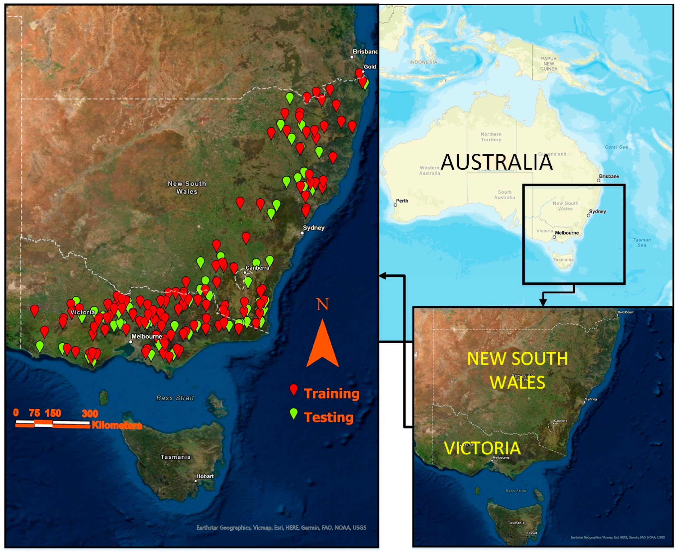
South-East Australia (Figure 1) was selected as the study area, since that part of Australia has high-quality streamflow data. The region is highly populated and has been impacted by numerous floods in the past. Catchments, which are natural and have at least 30 years of streamflow data, were selected for this study.
2.2. Data
A total of 181 catchments were selected for this study, as shown in Figure 1. The annual maximum (AM) flood data length of the selected stations ranged 40–89 years (mean: 48 years). The catchment sizes ranged 3–1010 km2 (mean: 349 km2). The selected catchments were divided into a training dataset (consisting of 126 catchments) and testing dataset (consisting of 55 catchments).
A total of eight predictor variables (Table 1) were selected as candidates [19], which were the catchment area (AREA), design rainfall intensity with a 6-h duration and 2-year return period (I62), mean annual rainfall (MAR), shape factor (SF), mean annual evapotranspiration (MAE), stream density (SDEN), mainstream slope S1085 and fraction forested area (FOREST). It should be noted that all these eight predictor variables were included in the developed ANN and SVM-based RFFA models presented in this study.
AREA is the main scaling factor and has widely been used in RFFA [52,53]. The design rainfall intensity is the main input to the flood generation process and has been adopted in many RFFA studies [50,54]. The minimum, maximum, average and median times of the concentration values of the selected catchments are 1.15 h, 10.53 h, 6.45 h and 6.67 h, respectively. The duration of the design rainfall is taken as six hours, which is closer to the average time of the concentration (6.45 h) of the selected catchments. To consider the shape of a catchment in RFFA, Rahman, Haddad [55] introduced SF, which is defined as the distance between the catchment centroid and outlet divided by the AREA. The MAE and MAR are surrogate to other characteristics affecting flood generation [56]; these are obtained at a catchment centroid from the Australian Bureau of Meteorology website. SDEN is another important factor in the flood generation process, which is calculated by dividing the total stream length within the catchment by AREA. FOREST is directly connected to the loss factor, the amount of water loss through infiltration during a flood event, and it also affects catchment roughness. S1085 is directly connected to the flood response (a higher slope means a higher flow velocity) and is defined by Equation (1) [19]:
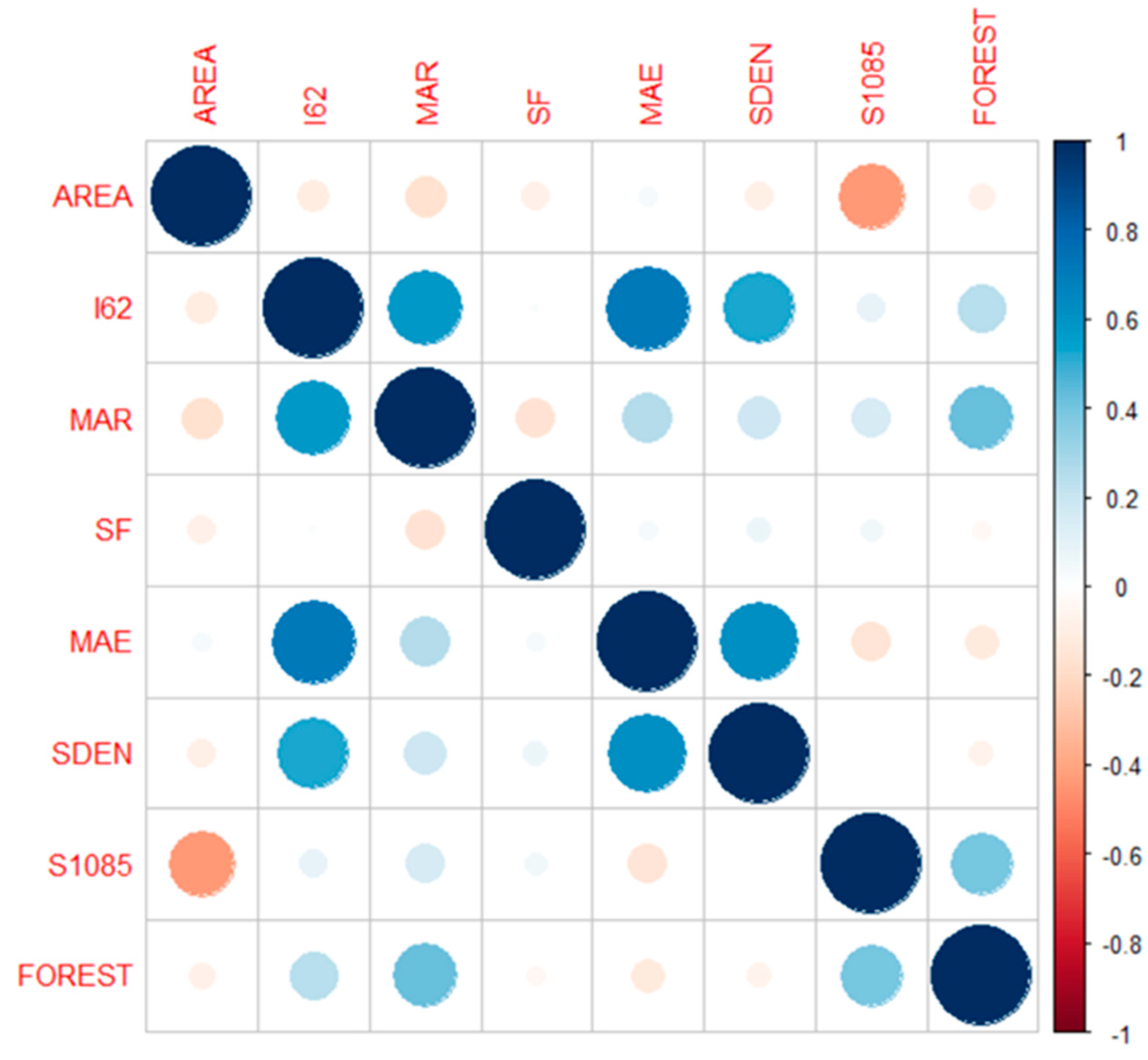
where H2 and H1 are elevations at 0.85 and 0.10 of the mainstream length, measured from the catchment outlet, and L is the mainstream length. Table 1 presents the summary of the selected predictor variables, and Figure 2 and Figure 3 present boxplots and correlation plots of the selected predictor variables.
The dependent variables in this study are flood quantiles for 2-year, 5-year, 10-year, 20-year, 50-year and 100-year return periods (Q2, Q5, Q10, Q20, Q50 and Q100, respectively). These are estimated by fitting a log-Pearson Type 3 (LP3) distribution to each of the selected station’s AM flood series. The parameters of the GEV distribution were estimated by the Bayesian method. It should be noted that other distributions such as GEV could have been used, but for South-East Australia, LP3 was found to be the best-fit probability distribution in previous FFA studies [50,54]. It should also be noted that the impacts of non-stationarity on the FFA results are worth considering [57], which, however, is beyond the scope of this study.
2.3. ANN-Based RFFA Method
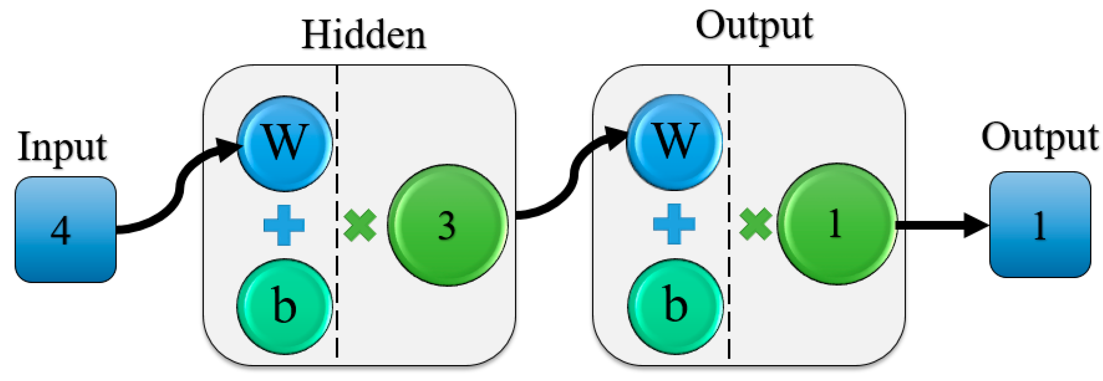
ANN is an empirical model capable of predicting flood quantiles using selected predictor variables [58]. The ANN modelling consists of three steps (model training, model testing and model evaluation). The evaluation is carried out using a set of statistical metrices, which compares predicted flood quantiles by the ANN model with the observed flood quantiles. This study uses a multi-layered feed-forward neural network consisting of an input layer with three to four nodes, a hidden layer and an output layer with one node, as shown in Figure 4 [59,60]. The optimum number of the hidden nodes and output nodes are selected according to a study conducted by Zhihua et al. [61].
There are four different types of training algorithms: Levenberg-Marquardt, Bayesian Regularization, Scaled Conjugate Gradient and Multilayer perceptron (MLP). First, the input nodes are filled with input variables. Hidden nodes are then connected to the input variables, and the initial weights are used to assign the synaptic connection between the input and hidden nodes and the hidden and output nodes. The initial weights are then replaced by random values of weights to start the training processes. These random values are used to generate normalised values, which are then used as new input nodes linked with hidden nodes [61]. The total sum of the input variables multiplied by the corresponding initial weights is activated to develop a MLR-type model [62]. The ANN method uses the following equation:
where z is a symbol for the graphical representation of ANN shown in Figure 4, wi is the weight coefficient and xi is the input or independent variable.
2.4. SVM-Based RFFA Method
The SVM method assumes that there is a relationship between the independent (I), and dependent (Q) variables via an additional parameter called noise (N), as shown below:
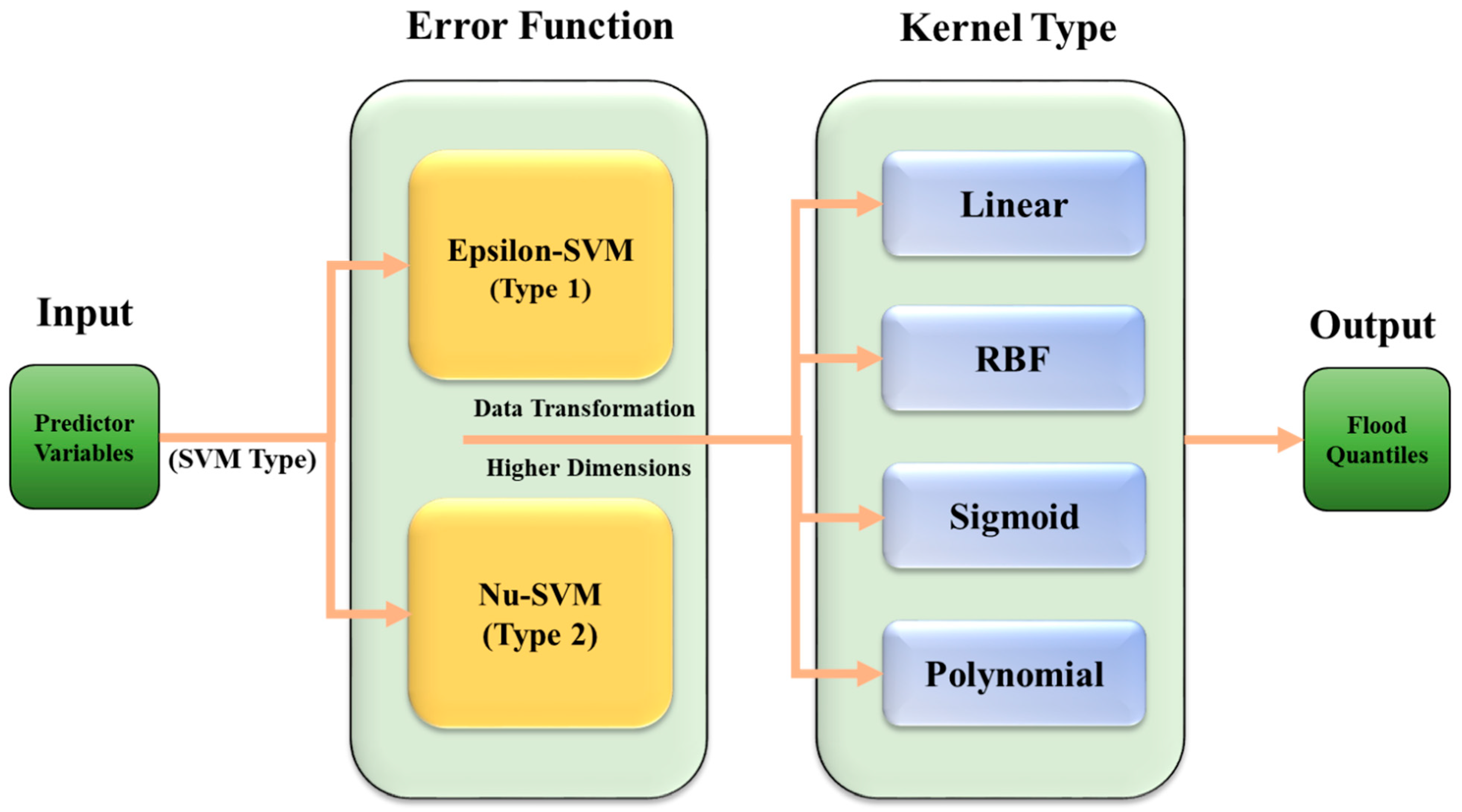
where the function (f) is developed based on available/measured data. This function could then be used to predict the flood quantile for an ungauged catchment using similar independent variables. Training an SVM model includes data classification and optimisation of an error function. A general process of an SVM method is shown in Figure 5. The method starts with a simple approach of finding the best formula, which simply connects the data and then calculates the error of the formula. The SVM methods are classified into two types based on two different types of error.
Q = f (I) + N
Error function type 1, epsilon-SVM, as shown in Equation (4):
where the subject is minimised using Equations (5) and (6):
where .
Error function type 2, also called Nu-SVM, uses Equation (7):
where the subject is minimised using Equations (8) and (9):
where .
Kernel Functions
Kernels are representative of the input data points in a higher dimensional feature space. Linear, polynomial, radial basis function (RBF) and sigmoid are some of the most common Kernel types used in SVM methods:
where is the kernel function. The gamma function can be used as a kernel function. The RBFs are common choices of kernel types, due to their localised and finite responses across the full domain of the real x-axis.
3. Statistical Metrices Used for Model Evaluation
Based on the results of the model testing on the selected 55 test catchments, the following metrices are used to compare the performances of the developed RFFA models [19]:
Abs REi = ABS(REi)
Qobs,i is at-site flood quantile (in m3/s) estimated by fitting LP3 distribution for each of the selected return periods at the site i (i = 1, N), and Qpred,i (in m3/s) is the predicted-flood quantiles using either SVM or ANN at site i. Here, N = 55, as there are 55 test catchments.
4. Results
The final predictor variables were selected based on their p-values (p-value must not exceed 0.10). The final predictor variables used are (i) AREA, I62, MAR and SDEN (for Q2); (ii) AREA, I62 and SDEN (for Q5 and Q10); (iii) AREA, I62, SDEN and MAR (for Q20 and Q50); and (iv) AREA, I62, MAE and MAR (for Q100). Table 2 shows the statistical metrices of the best ANN model for different flood quantiles. As shown in Appendix A (Table A1), the best methods were selected based on the most common evaluation statistics, such as MSE, RMSE, RRMSE, REr and Rbias. Table A1 shows some of the best-performing ANN methods with different algorithms; from these, the best one is presented in Table 2 and used for further investigation. Table A2 shows the different parameters used in developing the SVM methods, and Table A3 represents the best-performing SVM methods with different algorithms used in developing the SVM methods. The best-performing SVM methods are selected based on statistical indices and are represented in Table 3 and are used for further investigation. From Table 2, it can be seen that, for the ANN-based models, Q10 has the smallest Rbias and RMSNE values, whereas Q5 has the smallest REr value. From Table 3, it is found that Q2 has the smallest Rbias value, and Q5 has the smallest RMSNE value.
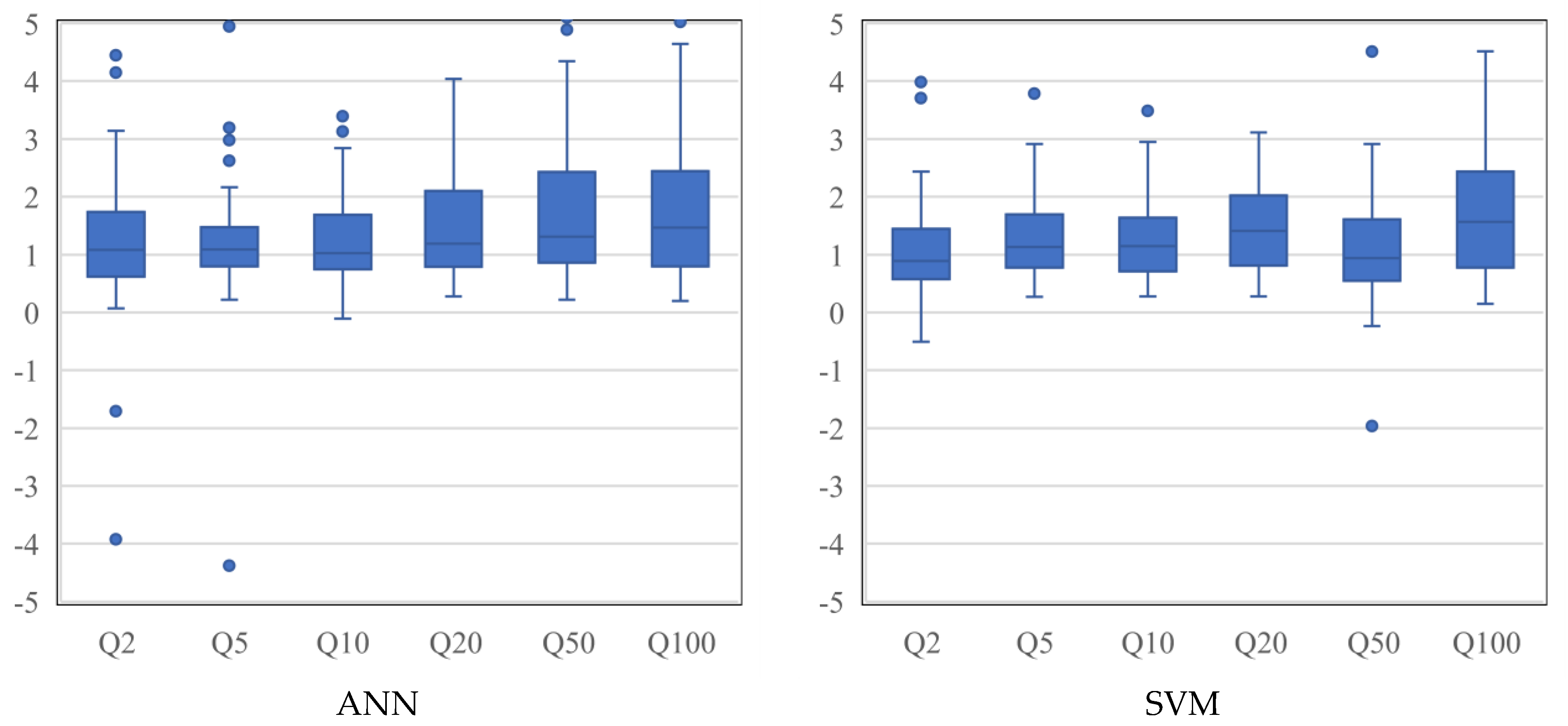
Figure 6 shows boxplot of Qratio values for ANN and SVM models. As can be seen in this figure, the ANN model shows some overestimation for Q20, Q50 and Q100, whereas, for the SVM model, there is an overestimation for Q20 and Q100. In terms of Qratio, the ANN presents better results for Q5 (with a smaller box width) as compared to SVM. As can be seen in Figure 6, the results of Q2 for SVM are better than the ANN. In terms of Q10, Q20 and Q100, both the models perform very similarly; however, the median values for SVM seem to be further away from the 1:1 line. The Qratio results for Q50 show that the SVM method has a better performance than the ANN, with a smaller box width and median value located near the 1:1 line Overall, the Q5 model for ANN is the best model (with the smallest box width), followed by Q10 (ANN), Q2 (SVM), Q5 (SVM), Q10 (SVM) and Q50 (SVM). For Q100, both the ANN and SVM and, for Q50, the ANN shows remarkable overestimations.
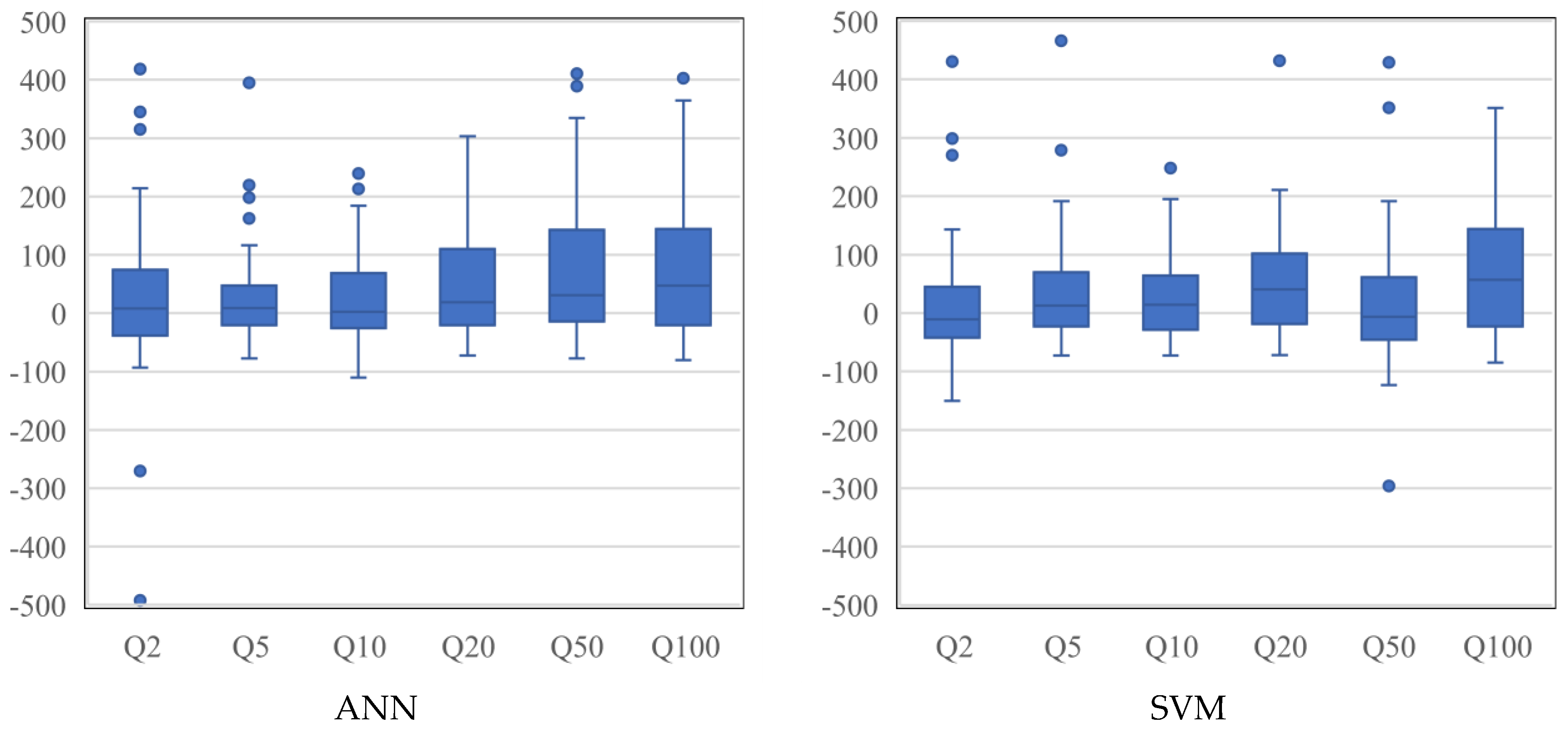
Figure 7 shows the boxplots of RE values for the ANN and SVM models. For Q2, SVM has a better performance, since it produces a smaller box width with a median value closer to the 0:0 line. The ANN produces better results for Q5 with a smaller box width. In terms of Q10, Q20 and Q100, both the models perform similarly; however, SVM produces better results for Q50. Overall, SVM shows better performance with smaller box widths. In terms of bias, Q5 (ANN), Q10 (ANN) and Q50 (SVM) present the best performances, as the median values are located closer to the 0:0 line. The Q100 model for both the ANN and SVM and Q50 (ANN) and Q20 (SVM) models produce notable overestimations. The best model is found for Q5 (ANN), followed by Q5 (SVM).
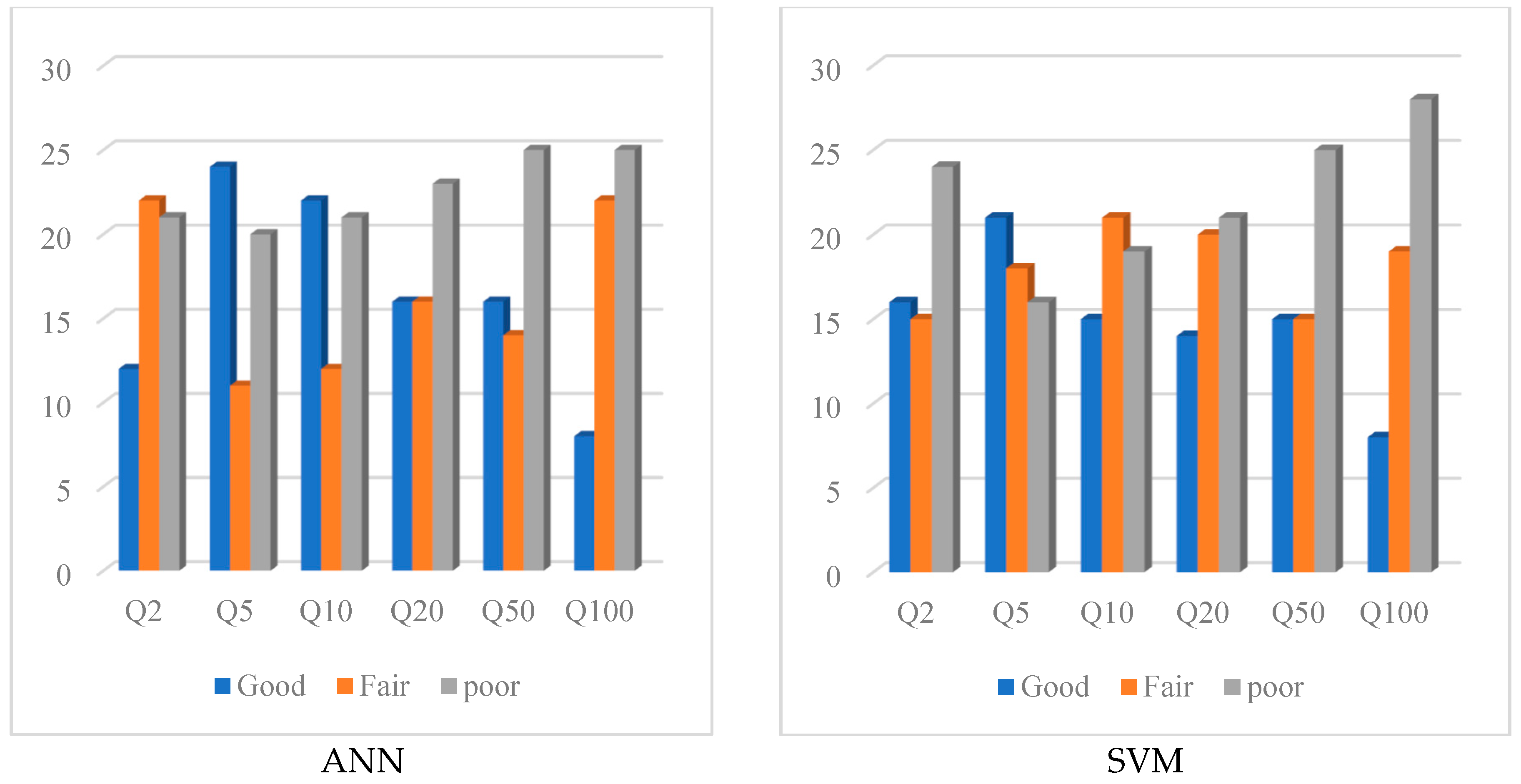
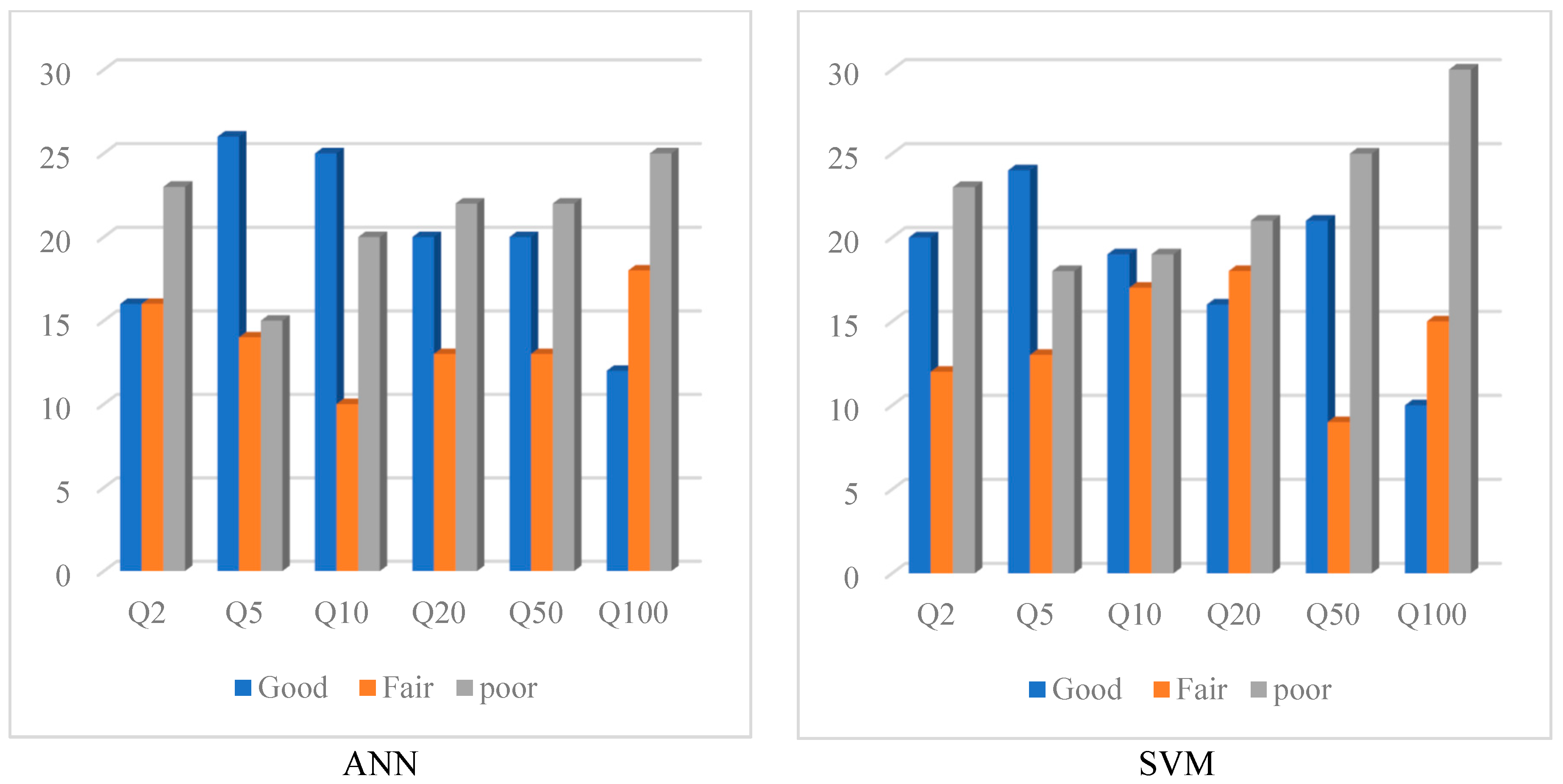
Figure 8 and Figure 9 show the qualitative comparison of the performance of the ANN and SVM methods based on the classification of the result in three groups (Good, Fair and Poor). These identifiers are used for different ranges of REr and Qratio values [63]. As seen in Figure 8, catchments with REr values falling in the range of 0–30% are rated as “Good”, catchments with REr values in the range of 31–60% are rated as “Fair” and “Poor” is assigned to the remaining catchments with REr values beyond 61%. Figure 7 shows the qualitative comparison of the performance of the ANN and SVM models for different test catchments based on Qratio. In this figure “Good” is assigned to the test catchments with the Qratio values falling between 0.8 and 1.3, “Fair” is assigned to the test catchments with Qratio values falling in the range of 0.6–0.79 and 1.31–2 and “Poor” is assigned to the remaining test catchments. The ANN method outperforms the SVM method in terms of REr values, because it has a Good-rated performance for more test catchments than SVM—in particular, for smaller return periods. Overall, both the SVM and ANN show a poor performance for Q100.
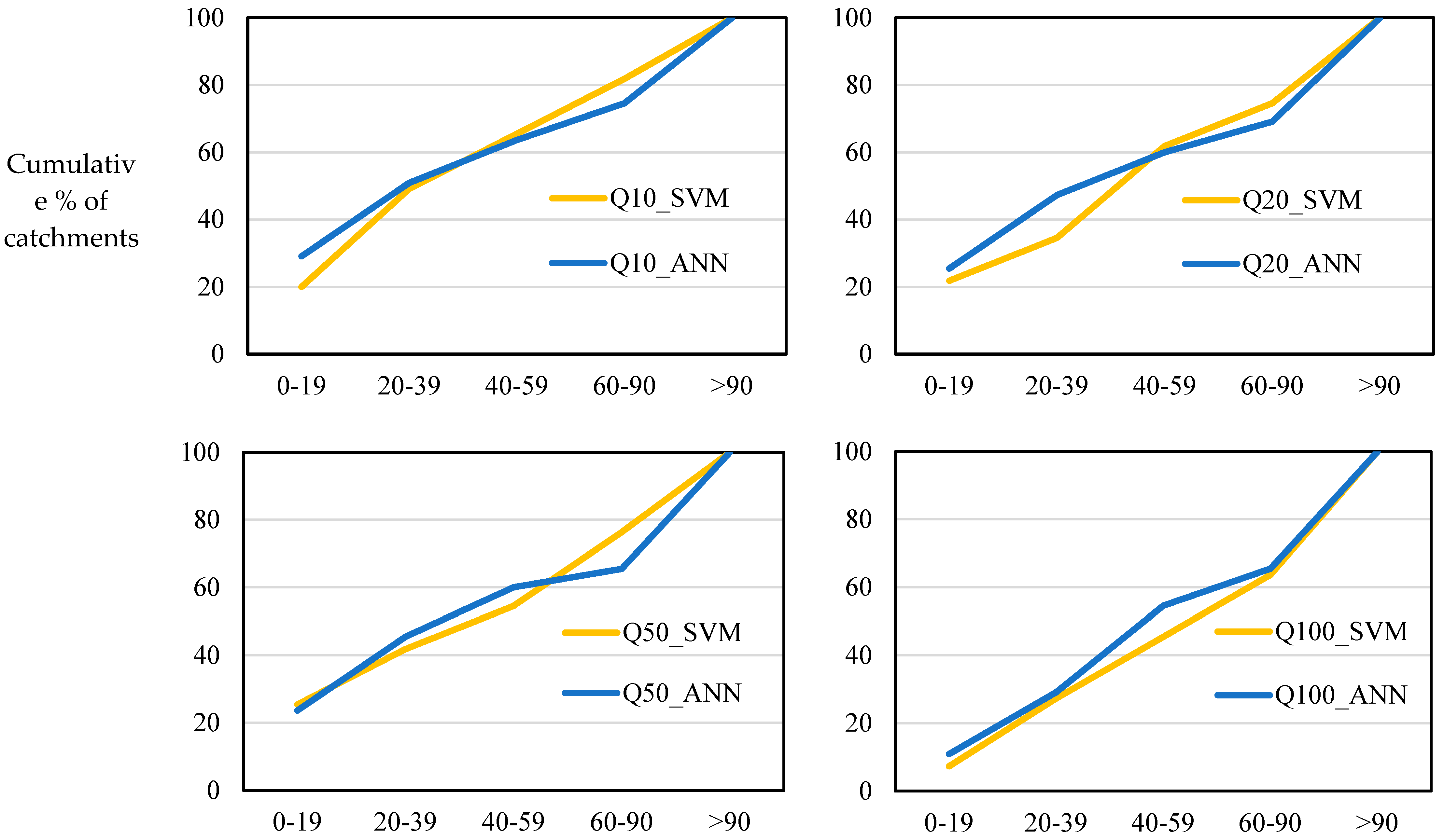
In terms of the cumulative percentage of stations based on Abs RE values, shown in Figure 10, both models perform very similarly, with the ANN method performing slightly better than the SVM for all the return periods, where the curve for ANN is above the SVM, except for Q2, showing that the ANN method performs better for a greater number of test catchments with lower ranges of Abs RE values.
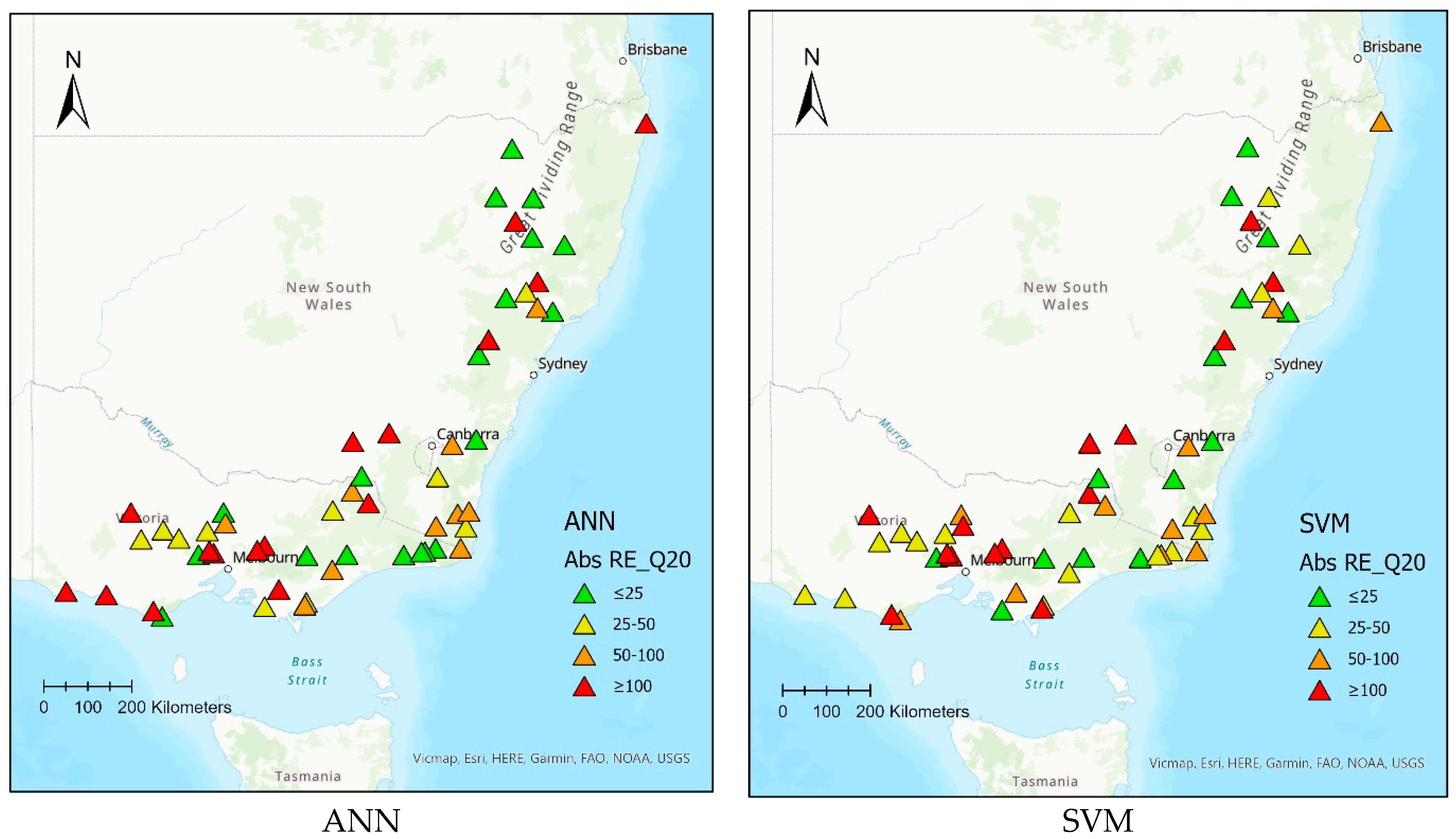
Figure 11 shows the performance of the ANN and SVM models based on Abs RE values for 55 test catchments over the geographical space for Q20 as an example. The ANN model performs better than the SVM, having 19 catchments with Abs RE values less than 25%, while there are only 14 catchments for the SVM method. There is no spatial pattern of the Abs RE values of the 55 test catchments.
Table 4 shows a comparison between the REr values for the ANN, SVM and the Australian Rainfall and Runoff (ARR) recommended RFFA model. REr values for the ANN method range 33.27–54.38%, which are smaller than those for the SVM (37.13–64.29%) and the ARR RFFA model (57.25–64.06%). It should be noted that the RFFA model was based on 558 stations from eastern Australia. Additionally, the ARR RFFA model used leave-one-out validation (as opposed to the split-sample validation adopted in this study), which generally generates a higher model error, because it is a more rigorous validation method. It should also be noted that the streamflow data lengths of the selected stations are much higher in the present study than the ARR RFFE model. This has given more advantage to the present study as compared to ARR RFFE model.
It should be noted that ARR RFFE model used only four predictor variables, whereas the ANN and SVM-based RFFA models in the present study used eight predictor variables. The use of higher number of predictor variables played a role in reducing the REr values associated with the ANN and SVM-based RFFA models; however, these models have higher bias than the ARR RFFE model [55]. Further investigation is needed to reduce the bias of these AI-based RFFA models.
The results of the present study are compared with similar ones. For example, Allahbakhshian-Farsani et al. [26] compared the results of the SVM, MARS, BRT, PPR and NLR methods and reported a RMSE value of 50.70 for their best-performing method (SVM); this value is 50.15 for the ANN-Q2 and 50.17 for the SVM-Q2 models in the present study. Similarly, Ghaderi et al. [44] reported a RMSE value of 239.94 for their best-performing method (SVM) when comparing it with the ANFIS and GEP methods. Vafakhah and Bozchaloei [28] compared the results of the ANN, SVM and NLR methods and reported a RRMSE of 1.45 for their best-performing method (SVM); these values were 0.79 and 0.80 for our ANN-Q5 and SVM-Q5 models, respectively. Ouarda and Shu [32] compared the results of the ANN method with MLR model and reported a RRMSE value of 36.17 and RMSE value of 27.33 for the ANN method as the best-performing method. Shu and Ouarda [31] used the ANFIS, ANN, NLR and NLR methods and reported RMSE and RRMSE values of 316 and 57, respectively, for their best-performing method. Jingyi and Hall [23] used cluster analysis and ANN methods and reported the best RMSE value of 47 for their best-performing method. The above discussion shows that the ANN and SVM models developed in the present study provided results similar to the relevant international studies.
5. Conclusions
In this study, the ANN-based RFFA models are compared with the SVM-based models. The performance of these two models varies with the return periods. Overall, based on the median relative error, the ANN outperforms the SVM. The best model is found to be for Q5 and Q10 with the ANN, giving the smallest median relative error (33–36%). This is notably smaller than the ARR-RFFE model (57%). It should be noted that the ARR-RFFE model adopted only four predictors, whereas the ANN and SVM-based models presented here adopted eight predictor variables, which played a role in reducing the prediction error.
For Q100, both the SVM and ARR-RFFE models provide similar relative errors (64%). In terms of bias, both the ANN and SVM models provide significant overestimations for Q100. This highlights that the estimation of floods with higher return periods is challenging. even with the artificial intelligence-based models.
A split-sample validation is adopted for comparing different models in the present study; in future studies, a Monte Carlo cross-validation should be adopted where the dataset can be randomly divided into numerous training and testing datasets. Furthermore, hybrid methods could be applied by combining different AI-based methods to reduce the prediction error and bias.
It should be noted that the relative accuracy of any RFFA technique depends on the quality and quantity of the streamflow and predictor variable data, which are used to develop and test the technique. For example, a short streamflow record length can introduce significant a sampling error in flood quantile estimates, which are used as a dependent variable in RFFA. Hence, the RFFA techniques examined in the present study should be repeated when a greater streamflow record length is available in the study area in the future. Furthermore, the impacts of climate change on RFFA need to be evaluated. The observed bias for the AI-based based RFFA models should be subjected to bias correction similar to the ARR RFFA technique, which, however, was not implemented here, as it needs further research.
Author Contributions
A.Z. conducted the data analysis and drafted the manuscript; A.R. supervised the research, assisted in interpreting the results and revised the manuscript; N.N. assisted in the data analysis, referencing and revising the manuscript; M.V. assisted in the data analysis and interpreting the results; B.S. edited and improved the manuscript and F.A. edited and enhanced the presentation. All authors have read and agreed to the published version of the manuscript.
Funding
This research received no external funding.
Data Availability Statement
The datasets used in this study can be obtained from the Australian Bureau of Meteorology, WaterNSW and Department of Environment, Land, Water and Planning of Victoria by paying a prescribed fee and/or from their websites (free of cost).
Acknowledgments
The authors would like to acknowledge the Australian Bureau of Meteorology, WaterNSW and Department of Environment, Land, Water and Planning of Victoria for providing the streamflow data used in this study. This study is part of the first author’s PhD research.
Conflicts of Interest
The authors declare that they have no conflicts of interest.
Appendix A

Table A1.
Ten best-performing ANN models for different flood quantiles.
| Q2 | Q5 | Q10 | Q20 | Q50 | Q100 | |||||||
|---|---|---|---|---|---|---|---|---|---|---|---|---|
| Sorted by performance | Network Name | Training Algorithm | Network Name | Training Algorithm | Network Name | Training Algorithm | Network Name | Training Algorithm | Network Name | Training Algorithm | Network Name | Training Algorithm |
| RBF 4-22-1 | RBFT | MLP 3-3-1 | BR | MLP 3-3-1 | BR | MLP 4-3-1 | LM | RBF 4-20-1 | RBFT | MLP 4-2-1 | LM | |
| MLP 4-8-1 | BFGS 63 | RBF 3-19-1 | RBFT | MLP 3-2-1 | LM | MLP 4-4-1 | LM | RBF 4-18-1 | RBFT | MLP 4-8-1 | LM | |
| MLP 4-3-1 | BR | MLP 3-7-1 | BFGS 34 | MLP 3-4-1 | BR | MLP 4-10-1 | LM | MLP 4-6-1 | LM | MLP 4-6-1 | LM | |
| MLP 4-2-1 | BFGS 43 | MLP 3-4-1 | BR | MLP 3-5-1 | LM | RBF 4-22-1 | RBFT | MLP 4-7-1 | LM | MLP 4-3-1 | BFGS 7 | |
| MLP 4-10-1 | LM | MLP 3-2-1 | BR | RBF 3-23-1 | RBFT | MLP 4-2-1 | LM | MLP 4-4-1 | LM | MLP 4-10-1 | LM | |
| MLP 4-6-1 | BFGS 109 | MLP 3-3-1 | LM | MLP 3-8-1 | LM | MLP 4-8-1 | LM | MLP 4-3-1 | LM | MLP 4-5-1 | BFGS 10 | |
| MLP 4-2-1 | BR | MLP 3-10-1 | BFGS 71 | MLP 3-3-1 | LM | MLP 4-9-1 | LM | MLP 4-9-1 | LM | MLP 4-9-1 | LM | |
| MLP 4-9-1 | LM | MLP 3-5-1 | BFGS 42 | MLP 3-4-1 | LM | MLP 4-7-1 | LM | MLP 4-2-1 | BR | RBF 4-18-1 | RBFT | |
| MLP 4-3-1 | SCG | MLP 3-6-1 | BFGS 61 | MLP 3-6-1 | BFGS 53 | MLP 4-6-1 | LM | MLP 4-5-1 | LM | RBF 4-19-1 | RBFT | |
| MLP 4-10-1 | BFGS 27 | MLP 3-5-1 | BR | MLP 3-9-1 | LM | MLP 4-5-1 | LM | MLP 4-10-1 | LM | MLP 4-3-1 | LM | |
Table A2.
Structures of the best-performing SVM models for different flood quantiles.
| Quantile | SVM Type | Kernel Type | Epsilon/Nu | Capacity | Gamma | Cross-Validation Error | Number of Support Vectors |
|---|---|---|---|---|---|---|---|
| Q2 | 1 | RBF | 0.200 | 10.000 | 0.250 | 0.038 | 22 (13 bounded) |
| Q5 | 1 | RBF | 0.100 | 6.000 | 0.333 | 0.050 | 45 (39 bounded) |
| Q10 | 1 | RBF | 0.100 | 10.000 | 0.333 | 0.053 | 59 (48 bounded) |
| Q20 | 2 | RBF | nu = 0.300 | 3.000 | 0.250 | 0.048 | 43 (33 bounded) |
| Q50 | 2 | Sigmoid | nu = 0.500 | 10.000 | 0.250 | 0.060 | 66 (61 bounded) |
| Q100 | 1 | RBF | 0.100 | 8.000 | 0.250 | 0.052 | 54 (42 bounded) |
Table A3.
Best-performing SVM models for different flood quantiles.
| Q2 | Q5 | Q10 | Q20 | Q50 | Q100 | |||||||
|---|---|---|---|---|---|---|---|---|---|---|---|---|
| Sorted by performance | Type(1) | RBF | Type(1) | RBF | Type(1) | RBF | Type(2) | RBF | Type(2) | Sigmoid | Type(1) | RBF |
| Type(2) | Polynomial | Type(2) | RBF | Type(2) | RBF | Type(2) | Sigmoid | Type(1) | Linear | Type(2) | Sigmoid | |
| Type(2) | RBF | Type(1) | Polynomial | Type(1) | Polynomial | Type(1) | Sigmoid | Type(1) | Polynomial | Type(2) | RBF | |
| Type(2) | Linear | Type(2) | Linear | Type(2) | Polynomial | Type(1) | RBF | Type(2) | Linear | Type(2) | Polynomial | |
| Type(1) | Polynomial | Type(2) | Polynomial | Type(1) | Sigmoid | Type(1) | Polynomial | Type(1) | Sigmoid | Type(1) | Polynomial | |
| Type(1) | Linear | Type(2) | Sigmoid | Type(2) | Sigmoid | Type(2) | Linear | Type(2) | Polynomial | Type(1) | Sigmoid | |
| Type(2) | Sigmoid | Type(1) | Linear | Type(2) | Linear | Type(2) | Polynomial | Type(1) | RBF | Type(1) | Linear | |
| Type(1) | Sigmoid | Type(1) | Sigmoid | Type(1) | Linear | Type(1) | Linear | Type(2) | RBF | Type(2) | Linear | |
References
- Nachappa, T.G.; Meena, S.R. A novel per pixel and object-based ensemble approach for flood susceptibility mapping. Geomat. Nat. Hazards Risk 2020, 11, 2147–2175. [Google Scholar] [CrossRef]
- Tsakiris, G. Flood risk assessment: Concepts, modelling, applications. Nat. Hazards Earth Syst. Sci. 2014, 14, 1361–1369. [Google Scholar] [CrossRef] [Green Version]
- Arrighi, C.; Tarani, F.; Vicario, E.; Castelli, F. Flood impacts on a water distribution network. Nat. Hazards Earth Syst. Sci. 2017, 17, 2109–2123. [Google Scholar] [CrossRef] [Green Version]
- Fekete, A. Critical infrastructure and flood resilience: Cascading effects beyond water. WIREs Water 2019, 6, e1370. [Google Scholar] [CrossRef] [Green Version]
- Rebally, A.; Valeo, C.; He, J.; Saidi, S. Flood Impact Assessments on Transportation Networks: A Review of Methods and Associated Temporal and Spatial Scales. Front. Sustain. Cities 2021, 3, 732181. [Google Scholar] [CrossRef]
- Kellermann, P.; Schöbel, A.; Kundela, G.; Thieken, A.H. Estimating flood damage to railway infrastructure—The case study of the March River flood in 2006 at the Austrian Northern Railway. Nat. Hazards Earth Syst. Sci. 2015, 15, 2485–2496. [Google Scholar] [CrossRef] [Green Version]
- De Ruiter, M.C.; Ward, P.J.; Daniell, J.E.; Aerts, J.C.J.H. Review Article: A comparison of flood and earthquake vulnerability assessment indicators. Nat. Hazards Earth Syst. Sci. 2017, 17, 1231–1251. [Google Scholar] [CrossRef] [Green Version]
- Yari, A.; Ardalan, A.; Ostadtaghizadeh, A.; Zarezadeh, Y.; Boubakran, M.S.; Bidarpoor, F.; Rahimiforoushani, A. Underlying factors affecting death due to flood in Iran: A qualitative content analysis. Int. J. Disaster Risk Reduct. 2019, 40, 101258. [Google Scholar] [CrossRef]
- Quintero, F.; Mantilla, R.; Anderson, C.; Claman, D.; Krajewski, W. Assessment of Changes in Flood Frequency Due to the Effects of Climate Change: Implications for Engineering Design. Hydrology 2018, 5, 19. [Google Scholar] [CrossRef] [Green Version]
- Cameron, D.; Beven, K.; Naden, P. Flood frequency estimation by continuous simulation under climate change (with uncertainty). Hydrol. Earth Syst. Sci. 2000, 4, 393–405. [Google Scholar] [CrossRef]
- Kollat, J.B.; Kasprzyk, J.R.; Thomas Jr, W.O.; Miller, A.C.; Divoky, D. Estimating the impacts of climate change and population growth on flood discharges in the United States. J. Water Resour. Plan. Manag. 2012, 138, 442–452. [Google Scholar] [CrossRef]
- Sanyal, J.; Densmore, A.L.; Carbonneau, P. Analysing the effect of land-use/cover changes at sub-catchment levels on downstream flood peaks: A semi-distributed modelling approach with sparse data. Catena 2014, 118, 28–40. [Google Scholar] [CrossRef] [Green Version]
- Hirabayashi, Y.; Mahendran, R.; Koirala, S.; Konoshima, L.; Yamazaki, D.; Watanabe, S.; Kim, H.; Kanae, S. Global flood risk under climate change. Nat. Clim. Chang. 2013, 3, 816–821. [Google Scholar] [CrossRef]
- Mishra, A.; Alnahit, A.; Campbell, B. Impact of land uses, drought, flood, wildfire, and cascading events on water quality and microbial communities: A review and analysis. J. Hydrol. 2020, 596, 125707. [Google Scholar] [CrossRef]
- Ligtvoet, W.; Hilderink, H.; Bouwman, A.; Puijenbroek, P.; Lucas, P.; Witmer, M. Towards a World of Cities in 2050. An Outlook on Water-Related Challenges; Background report to the UN-Habitat Global Report; PBL Netherlands Environmental Assessment Agency: The Hague, The Netherlands, 2014. [Google Scholar]
- Kirkup, H.; Brierley, G.; Brooks, A.; Pitman, A. Temporal variability of climate in south-eastern Australia: A reassessment of flood-and drought-dominated regimes. Aust. Geogr. 1998, 29, 241–255. [Google Scholar] [CrossRef]
- Halgamuge, M.N.; Nirmalathas, A. Analysis of large flood events: Based on flood data during 1985–2016 in Australia and India. Int. J. Disaster Risk Reduct. 2017, 24, 1–11. [Google Scholar] [CrossRef]
- Johnson, F.; White, C.J.; van Dijk, A.; Ekstrom, M.; Evans, J.P.; Jakob, D.; Kiem, A.S.; Leonard, M.; Rouillard, A.; Westra, S. Natural hazards in Australia: Floods. Clim. Chang. 2016, 139, 21–35. [Google Scholar] [CrossRef] [Green Version]
- Zalnezhad, A.; Rahman, A.; Vafakhah, M.; Samali, B.; Ahamed, F. Regional Flood Frequency Analysis Using the FCM-ANFIS Algorithm: A Case Study in South-Eastern Australia. Water 2022, 14, 1608. [Google Scholar] [CrossRef]
- Hosking, J.R.M.; Wallis, J.R. Regional Frequency Analysis: An Approach Based on L-Moments; Cambridge University Press: Cambridge, UK, 1997. [Google Scholar] [CrossRef]
- Shu, C.; Burn, D.H. Artificial neural network ensembles and their application in pooled flood frequency analysis. Water Resour. Res. 2004, 40. [Google Scholar] [CrossRef]
- Aziz, K.; Rahman, A.; Shamseldin, A. Development of Artificial Intelligence Based Regional Flood Estimation Techniques for Eastern Australia. In Artificial Neural Network Modelling; Springer: Berlin/Heidelberg, Germany, 2016; pp. 307–323. [Google Scholar] [CrossRef]
- Jingyi, Z.; Hall, M. Regional flood frequency analysis for the Gan-Ming River basin in China. J. Hydrol. 2004, 296, 98–117. [Google Scholar] [CrossRef]
- Garmdareh, E.S.; Vafakhah, M.; Eslamian, S.S. Regional flood frequency analysis using support vector regression in arid and semi-arid regions of Iran. Hydrol. Sci. J. 2018, 63, 426–440. [Google Scholar] [CrossRef]
- Gizaw, M.S.; Gan, T.Y. Regional Flood Frequency Analysis using Support Vector Regression under historical and future climate. J. Hydrol. 2016, 538, 387–398. [Google Scholar] [CrossRef]
- Allahbakhshian-Farsani, P.; Vafakhah, M.; Khosravi-Farsani, H.; Hertig, E. Regional Flood Frequency Analysis Through Some Machine Learning Models in Semi-arid Regions. Water Resour. Manag. 2020, 34, 1–23. [Google Scholar] [CrossRef]
- Linh, N.T.T.; Ruigar, H.; Golian, S.; Bawoke, G.T.; Gupta, V.; Rahman, K.U.; Sankaran, A.; Pham, Q.B. Flood prediction based on climatic signals using wavelet neural network. Acta Geophys. 2021, 69, 1413–1426. [Google Scholar] [CrossRef]
- Vafakhah, M.; Bozchaloei, S.K. Regional Analysis of Flow Duration Curves through Support Vector Regression. Water Resour. Manag. 2019, 34, 283–294. [Google Scholar] [CrossRef]
- Dawson, C.; Abrahart, R.; Shamseldin, A.; Wilby, R. Flood estimation at ungauged sites using artificial neural networks. J. Hydrol. 2006, 319, 391–409. [Google Scholar] [CrossRef] [Green Version]
- Shu, C.; Ouarda, T.B.M.J. Flood frequency analysis at ungauged sites using artificial neural networks in canonical correlation analysis physiographic space. Water Resour. Res. 2007, 43. [Google Scholar] [CrossRef] [Green Version]
- Shu, C.; Ouarda, T. Regional flood frequency analysis at ungauged sites using the adaptive neuro-fuzzy inference system. J. Hydrol. 2008, 349, 31–43. [Google Scholar] [CrossRef]
- Ouarda, T.B.M.J.; Shu, C. Regional low-flow frequency analysis using single and ensemble artificial neural networks. Water Resour. Res. 2009, 45, 11. [Google Scholar] [CrossRef]
- Aziz, K.; Rahman, A.; Fang, G.; Shrestha, S. Application of artificial neural networks in regional flood frequency analysis: A case study for Australia. Stoch. Hydrol. Hydraul. 2013, 28, 541–554. [Google Scholar] [CrossRef]
- Alobaidi, M.H.; Marpu, P.R.; Ouarda, T.B.; Chebana, F. Regional frequency analysis at ungauged sites using a two-stage resampling generalized ensemble framework. Adv. Water Resour. 2015, 84, 103–111. [Google Scholar] [CrossRef]
- Durocher, M.; Chebana, F.; Ouarda, T.B.M.J. A Nonlinear Approach to Regional Flood Frequency Analysis Using Projection Pursuit Regression. J. Hydrometeorol. 2015, 16, 1561–1574. [Google Scholar] [CrossRef]
- Chokmani, K.; Ouarda, T.B.M.J. Physiographical space-based kriging for regional flood frequency estimation at ungauged sites. Water Resour. Res. 2004, 40, 12. [Google Scholar] [CrossRef]
- Wazneh, H.; Chebana, F.; Ouarda, T.B.M.J. Optimal depth-based regional frequency analysis. Hydrol. Earth Syst. Sci. 2013, 17, 2281–2296. [Google Scholar] [CrossRef] [Green Version]
- Chebana, F.; Charron, C.; Ouarda, T.B.M.J.; Martel, B. Regional Frequency Analysis at Ungauged Sites with the Generalized Additive Model. J. Hydrometeorol. 2014, 15, 2418–2428. [Google Scholar] [CrossRef] [Green Version]
- Nezhad, M.K.; Chokmani, K.; Ouarda, T.B.M.J.; Barbet, M.; Bruneau, P. Regional flood frequency analysis using residual kriging in physiographical space. Hydrol. Process. 2010, 24, 2045–2055. [Google Scholar] [CrossRef]
- Aziz, K.; Rai, S.; Rahman, A. Design flood estimation in ungauged catchments using genetic algorithm-based artificial neural network (GAANN) technique for Australia. Nat. Hazards 2015, 77, 805–821. [Google Scholar] [CrossRef]
- Ouali, D.; Chebana, F.; Ouarda, T.B.M.J. Fully nonlinear statistical and machine-learning approaches for hydrological frequency estimation at ungauged sites. J. Adv. Model. Earth Syst. 2017, 9, 1292–1306. [Google Scholar] [CrossRef]
- Ouarda, T.B.; Girard, C.; Cavadias, G.S.; Bobée, B. Regional flood frequency estimation with canonical correlation analysis. J. Hydrol. 2001, 254, 157–173. [Google Scholar] [CrossRef]
- Ouali, D.; Chebana, F.; Ouarda, T.B.M.J. Non-linear canonical correlation analysis in regional frequency analysis. Stoch. Hydrol. Hydraul. 2015, 30, 449–462. [Google Scholar] [CrossRef]
- Ghaderi, K.; Motamedvaziri, B.; Vafakhah, M.; Dehghani, A.A. Regional flood frequency modeling: A comparative study among several data-driven models. Arab. J. Geosci. 2019, 12, 588. [Google Scholar] [CrossRef]
- Haddad, K.; Rahman, A. Regional flood frequency analysis: Evaluation of regions in cluster space using support vector regression. Nat. Hazards 2020, 102, 489–517. [Google Scholar] [CrossRef]
- Kordrostami, S.; Alim, M.; Karim, F.; Rahman, A. Regional Flood Frequency Analysis Using an Artificial Neural Network Model. Geosciences 2020, 10, 127. [Google Scholar] [CrossRef] [Green Version]
- Desai, S.; Ouarda, T.B. Regional hydrological frequency analysis at ungauged sites with random forest regression. J. Hydrol. 2020, 594, 125861. [Google Scholar] [CrossRef]
- Bozchaloei, S.K.; Vafakhah, M. Regional Analysis of Flow Duration Curves Using Adaptive Neuro-Fuzzy Inference System. J. Hydrol. Eng. 2015, 20, 06015008. [Google Scholar] [CrossRef]
- Kumar, R.; Goel, N.K.; Chatterjee, C.; Nayak, P.C. Regional Flood Frequency Analysis using Soft Computing Techniques. Water Resour. Manag. 2015, 29, 1965–1978. [Google Scholar] [CrossRef]
- Haddad, K.; Rahman, A. Regional flood frequency analysis in eastern Australia: Bayesian GLS regression-based methods within fixed region and ROI framework–Quantile Regression vs. Parameter Regression Technique. J. Hydrol. 2012, 430, 142–161. [Google Scholar] [CrossRef]
- Zalnezhad, A.; Rahman, A.; Nasiri, N.; Haddad, K.; Rahman, M.M.; Vafakhah, M.; Samali, B.; Ahamed, F. Artificial Intelligence-Based Regional Flood Frequency Analysis Methods: A Scoping Review. Water 2022, 14, 2677. [Google Scholar] [CrossRef]
- Anderson, H.W. Relating sediment yield to watershed variables. Trans. Am. Geophys. Union 1957, 38, 921–924. [Google Scholar] [CrossRef]
- Rahman, A. Flood Estimation for Ungauged Catchments: A Regional Approach Using Flood and Catchment Characteristics. Unpublished Ph.D. Thesis, Department of Civil Engineering, Monash University, Melbourne, Australia, 1997. [Google Scholar]
- Rahman, A.; Haddad, K.; Kuczera, G.; Weinmann, E. Regional flood methods. In Australian Rainfall and Runoff: A Guide To Flood Estimation. Book 3, Peak Flow Estimation; Commonwealth of Australia: Canberra, Australia, 2019; pp. 105–146. [Google Scholar]
- Rahman, A.; Haddad, K.; Haque, M.; Kuczera, G.; Weinmann, P. Australian Rainfall and Runoff Project 5: Regional Flood Methods: Stage 3 Report; Technical Report; Engineers Australia: Canberra, Australia, 2015. [Google Scholar]
- Zhang, L.; Hickel, K.; Dawes, W.R.; Chiew, F.H.S.; Western, A.W.; Briggs, P.R. A rational function approach for estimating mean annual evapotranspiration. Water Resour. Res. 2004, 40, 89–97. [Google Scholar] [CrossRef]
- Aksu, H.; Cetin, M.; Aksoy, H.; Yaldiz, S.G.; Yildirim, I.; Keklik, G. Spatial and temporal characterization of standard duration-maximum precipitation over Black Sea Region in Turkey. Nat. Hazards 2022, 111, 2379–2405. [Google Scholar] [CrossRef]
- Daliakopoulos, I.N.; Tsanis, I.K. Comparison of an artificial neural network and a conceptual rainfall–runoff model in the simulation of ephemeral streamflow. Hydrol. Sci. J. 2016, 61, 2763–2774. [Google Scholar] [CrossRef]
- Kan, G.; Liang, K.; Yu, H.; Sun, B.; Ding, L.; Li, J.; He, X.; Shen, C. Hybrid machine learning hydrological model for flood forecast purpose. Open Geosci. 2020, 12, 813–820. [Google Scholar] [CrossRef]
- Chen, C.; Hui, Q.; Xie, W.; Wan, S.; Zhou, Y.; Pei, Q. Convolutional Neural Networks for forecasting flood process in Internet-of-Things enabled smart city. Comput. Networks 2020, 186, 107744. [Google Scholar] [CrossRef]
- Lv, Z.; Zuo, J.; Rodriguez, D. Predicting of Runoff Using an Optimized SWAT-ANN: A Case Study. J. Hydrol. Reg. Stud. 2020, 29, 100688. [Google Scholar] [CrossRef]
- Chan, V.K.; Chan, C.W. Towards explicit representation of an artificial neural network model: Comparison of two artificial neural network rule extraction approaches. Petroleum 2019, 6, 329–339. [Google Scholar] [CrossRef]
- Rahman, A.S.; Khan, Z.; Rahman, A. Application of independent component analysis in regional flood frequency analysis: Comparison between quantile regression and parameter regression techniques. J. Hydrol. 2020, 581, 124372. [Google Scholar] [CrossRef]
Figure 1.
Study area and selected catchments.

Figure 2.
Boxplots of candidate eight predictor variables.

Figure 3.
Correlations among eight candidate predictor variables.

Figure 4.
ANN structure.

Figure 5.
SVM structure.

Figure 6.
Boxplot of Qratio values for the ANN and SVM methods. Y-axis presents Qratio values.

Figure 7.
RE for the ANN and SVM methods (y-axis represents RE in %).

Figure 8.
Number of stations (testing dataset) based on Qratio for the ANN and SVM models.

Figure 9.
Number of stations (testing dataset) based on REr values for the ANN and SVM models.

Figure 10.
Plot of cumulative percentage of stations based on Abs RE values for SVM and ANN models.


Figure 11.
Spatial distribution of Abs RE values for ANN-Q20 and SVM-Q20 for 55 selected test catchments.
Figure 11.
Spatial distribution of Abs RE values for ANN-Q20 and SVM-Q20 for 55 selected test catchments.

Table 1.
Summary of the candidate predictor variables based on 181 study catchments.
| Predictor Variable | Name of Variable | Unit | Statistical Parameter | |||
|---|---|---|---|---|---|---|
| Minimum | Maximum | Mean | Median | |||
| AREA | Catchment area | km2 | 3.00 | 1010.00 | 349.06 | 304.00 |
| I62 | Design rainfall intensity with 6-h duration and 2-year return period | mm/h | 24.60 | 87.30 | 39.03 | 37.30 |
| MAR | Mean annual rainfall | mm | 484.39 | 1953.23 | 970.50 | 910.37 |
| SF | Shape factor | - | 0.25 | 1.62 | 0.78 | 0.78 |
| MAE | Mean annual evapotranspiration | mm | 925.90 | 1543.30 | 1112.74 | 1071.90 |
| SDEN | Stream density | km−1 | 0.51 | 5.47 | 2.06 | 1.61 |
| S1085 | Slope of central 75% of the mainstream | m/km | 0.80 | 69.90 | 13.02 | 9.40 |
| FOREST | Fraction forest | - | 0.00 | 1.00 | 0.55 | 0.59 |
Table 2.
Statistical evaluations of the best-performing ANN model for different quantiles.
| Quantile | Network Name | Training Algorithm | Median Ratio | MSE | RMSE | RRMSE | REr | Rbias | RMSNE |
|---|---|---|---|---|---|---|---|---|---|
| Q2 | RBF 4-22-1 | RBFT | 1.01 | 2514.63 | 50.15 | 0.82 | 41.97 | 117.37 | 4.57 |
| Q5 | MLP 3-3-1 | BR | 1.09 | 14,523.69 | 120.51 | 0.79 | 33.27 | 57.65 | 2.67 |
| Q10 | MLP 3-3-1 | BR | 1.02 | 38,852.75 | 197.11 | 0.80 | 36.10 | 24.20 | 2.28 |
| Q20 | MLP 4-3-1 | LM | 1.19 | 104,981.21 | 324.01 | 0.89 | 40.45 | 150.56 | 5.61 |
| Q50 | RBF 4-20-1 | RBFT | 1.31 | 267,171.25 | 516.89 | 0.90 | 44.90 | 141.24 | 3.54 |
| Q100 | MLP 4-2-1 | LM | 1.47 | 639,427.42 | 799.64 | 1.02 | 54.38 | 145.03 | 4.18 |
Table 3.
Statistical evaluations of the best-performing SVM model for different quantiles.
| Quantile | SVM Type | Kernel Type | Median Ratio | MSE | RMSE | RRMSE | REr | Rbias | RMSNE |
|---|---|---|---|---|---|---|---|---|---|
| Q2 | 1 | RBF | 0.89 | 2516.95 | 50.17 | 0.82 | 42.79 | −32.79 | 2.84 |
| Q5 | 1 | RBF | 1.13 | 14,886.86 | 122.01 | 0.80 | 37.13 | 75.43 | 2.51 |
| Q10 | 1 | RBF | 1.14 | 39,363.88 | 198.40 | 0.81 | 41.01 | 103.89 | 3.54 |
| Q20 | 2 | RBF | 1.41 | 92,444.54 | 304.05 | 0.84 | 46.70 | 94.47 | 2.73 |
| Q50 | 2 | Sigmoid | 0.94 | 536,655.49 | 732.57 | 1.28 | 45.45 | −43.70 | 5.08 |
| Q100 | 1 | RBF | 1.57 | 611,790.05 | 782.17 | 1.00 | 64.29 | 166.96 | 4.31 |
Table 4.
Comparison of the REr values between the ARR RFFA, SVM and ANN models.
| Quantiles | ARR RFFA Model REr | SVM-REr | ANN-REr |
|---|---|---|---|
| Q2 | 63.07 | 42.79 | 41.97 |
| Q5 | 57.25 | 37.13 | 33.27 |
| Q10 | 57.48 | 41.01 | 36.10 |
| Q20 | 58.85 | 46.70 | 40.45 |
| Q50 | 60.39 | 45.45 | 44.90 |
| Q100 | 64.06 | 64.29 | 54.38 |
Publisher’s Note: MDPI stays neutral with regard to jurisdictional claims in published maps and institutional affiliations. |
© 2022 by the authors. Licensee MDPI, Basel, Switzerland. This article is an open access article distributed under the terms and conditions of the Creative Commons Attribution (CC BY) license (https://creativecommons.org/licenses/by/4.0/).
Share and Cite
MDPI and ACS Style
Zalnezhad, A.; Rahman, A.; Nasiri, N.; Vafakhah, M.; Samali, B.; Ahamed, F. Comparing Performance of ANN and SVM Methods for Regional Flood Frequency Analysis in South-East Australia. Water 2022, 14, 3323. https://doi.org/10.3390/w14203323
AMA Style
Zalnezhad A, Rahman A, Nasiri N, Vafakhah M, Samali B, Ahamed F. Comparing Performance of ANN and SVM Methods for Regional Flood Frequency Analysis in South-East Australia. Water. 2022; 14(20):3323. https://doi.org/10.3390/w14203323
Chicago/Turabian StyleZalnezhad, Amir, Ataur Rahman, Nastaran Nasiri, Mehdi Vafakhah, Bijan Samali, and Farhad Ahamed. 2022. "Comparing Performance of ANN and SVM Methods for Regional Flood Frequency Analysis in South-East Australia" Water 14, no. 20: 3323. https://doi.org/10.3390/w14203323
Note that from the first issue of 2016, this journal uses article numbers instead of page numbers. See further details here.