Article

Budyko-Type Models and the Proportionality Hypothesis in Long-Term Water and Energy Balances

by
Fernando Paz Pellat
1,
Jaime Garatuza Payán
2,
Víctor Salas Aguilar
3,
Alma Socorro Velázquez Rodríguez
4 and
Martín Alejandro Bolaños González
5,*
1
Mexican Carbon Program, Chiconautla Street No. 8, Lomas de Cristo, Texcoco CP 56225, Mexico
2
Department of Water and Environmental Sciences, Technological Institute of Sonora, Obregon City 85000, Mexico
3
Geoinformatics, Autonomous University of Ciudad Juarez, Km. 3.5, Anáhuac Highway, Cuauhtémoc, Chihuahua 31600, Mexico
4
Science Faculty, Campus El Cerrillo, Autonomous Mexico State University, Instituto Literario, # 100. C.P. 50000 Centro, Toluca 50000, Mexico
5
Hydrosciences, Postgraduate College, Campus Montecillo, México-Texcoco Highway Km 36.5, Montecillo 56230, Mexico
*
Author to whom correspondence should be addressed.
Water 2022, 14(20), 3315; https://doi.org/10.3390/w14203315
Submission received: 18 September 2022 / Revised: 6 October 2022 / Accepted: 14 October 2022 / Published: 20 October 2022
(This article belongs to the Section Hydrology)

Abstract

:
In the perspective of Darwinian hydrology, Budyko hypotheses can be the foundation of approaches for developing models. Numerous Budyko-type models meeting established boundary conditions (water and energy limits) have been developed based on the Budyko hypothesis on the long-term-average annual mass and energy balance. Some of these models are grounded on empirical bases, while others have been formulated on sophisticated mathematical developments. We analyze the basic hypotheses underlying some Budyko-type models; we first describe some published models and then examine their underlying hypotheses in a hydrologically intuitive space (precipitation versus runoff). The analyses show that the models studied are a consequence of assuming that two parallel straight lines (of unit slope) of different intercepts are indeed equal (proportionality hypothesis). This hypothesis gives rise to different Budyko-type models that, although mathematically correct and meeting the limits (partially) related to the Budyko hypotheses, do not yield any information about what happens between those limits. To overcome the extreme energy limit, an expolinear model is introduced.

1. Introduction

Water and energy balances in catchments are primary approaches for developing hydrological models. Modeling the precipitation-runoff relationship is a basic process for operational applications in hydrology. Hydrological modeling over long time periods (e.g., years) and large areas (e.g., catchments) was introduced by [1] using a global (top down) approach for studying hydrological responses; such an approach was subsequently expanded by [2]. Global modeling offers the advantage of reducing the number of parameters and data requirements by limiting model complexity [3]. The alternative of using physical process-based hydrological models such as the Soil and Water Assessment Tool (SWAT) [4] demands information that is frequently not available, as well as a vast amount of input data to describe the precipitation and actual evapotranspiration fields, soil hydraulic properties, vegetation characteristics, topography, etc., for properly representing hydrological processes.
Such an approach which explicitly considers hydrological processes (infiltration, storage, evaporation, etc.) and their associated parameterization, is called Newtonian (bottom-up approach), as opposed to the global or Darwinian approach [5] that starts by recognizing general patterns or laws at the aggregate level and then seeks to disaggregate them by introducing new variables as the space-time scale changes (top-down approach). A classic example of the Darwinian approach is the [6] hypothesis on the partitioning of precipitation in catchments for long-term average annual conditions. Budyko-type functional relationships [7] that meet the limits set by [6] have boomed in recent years, particularly because evapotranspiration (E) can be readily estimated from precipitation (P) and potential evapotranspiration (Eo) data, which are usually available for most catchments. In addition to the empirical approaches to Budyko-type relationships, relatively complex mathematical approaches have also been used to derive and justify relationships that are similar to the empirical counterparts [8,9,10,11,12]. Those methods have used theoretical approaches based on sound mathematical considerations that add credibility to the resultant Budyko-type relationships. However, from the perspective of conceptualizing and developing sound theories based on hydrological criteria, the mathematical soundness of a hydrological model is not sufficient to warrant its validity. According to [13], “For a good mathematical model it is not enough to work well. It must work well for the right reasons”. This same author pointed out that using mathematical tools in hydrological modeling is useful for hydrological concepts as well as for misconceptions. The objective of this work is to review the most used [7] Budyko-type relationships (precipitation-runoff) that have been derived in a mathematically rigorous fashion but by using a more intuitive and simple graphic and algebraic format in order to reach similar outcomes and reveal the hypotheses implicitly made in the developments analyzed. First, we review the original Budyko hypotheses, as well as the hypotheses and empirical relationships that have been proposed or derived afterwards. We then analyze some Budyko-type relationships, clarifying their implications. It is important to note that the Budyko hypotheses (limits) are not questioned in this paper, but rather the models derived from them: Budyko-type functional relationships. The main objective of this review is to put the different Budyko-type models in a similar format to understand their hypotheses (proportionality) and theoretical bases. The review does not discuss the bases or developments of the different models analyzed, but rather their mathematical structure. This approach can be used to extend the analysis to other Budyko type models to explore if a proportionality hypothesis is used. In addition, it does not pretend novelties in the representation of the models, but to facilitate their understanding in intuitive spaces. Regardless, a new Budyko model is introduced and generalization schemes are proposed from the daily to the annual long-term scale.

2. Budyko-Type Functional Relationships

Considering long-term-average annual values of the energy-mass balance, precipitation in a catchment can be partitioned as follows:
P = E + Q
where Q is runoff. Equation (1) assumes that soil storage is negligible. Equation (1), the continuity equation for a given temporal and spatial scale, is the foundation of hydrological analysis and can be regarded as a fundamental theorem [14]. Equation (1) can be rewritten by dividing both sides by P, as:
1 = E P + Q P
which allows relating E/P with Q/P by using ratios.

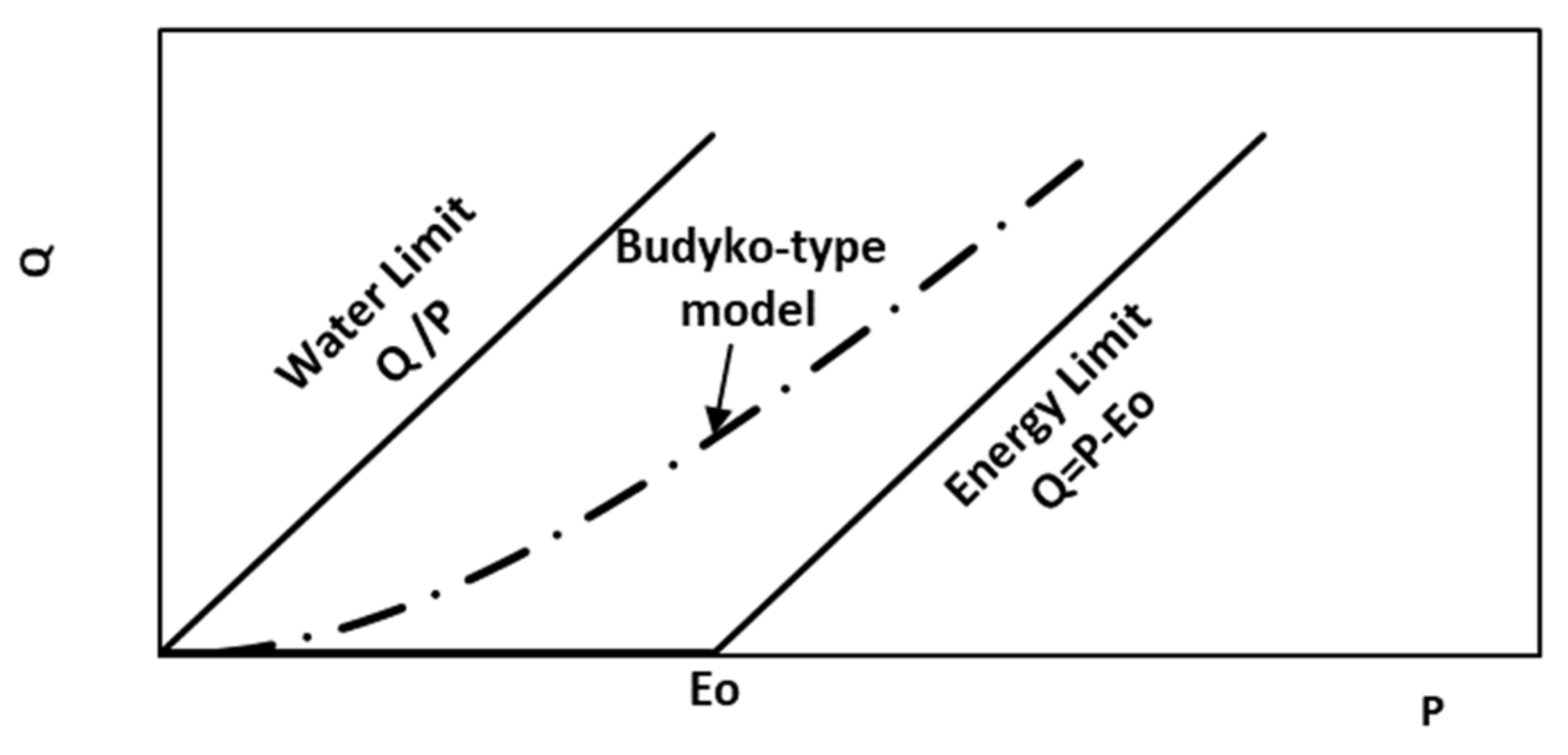
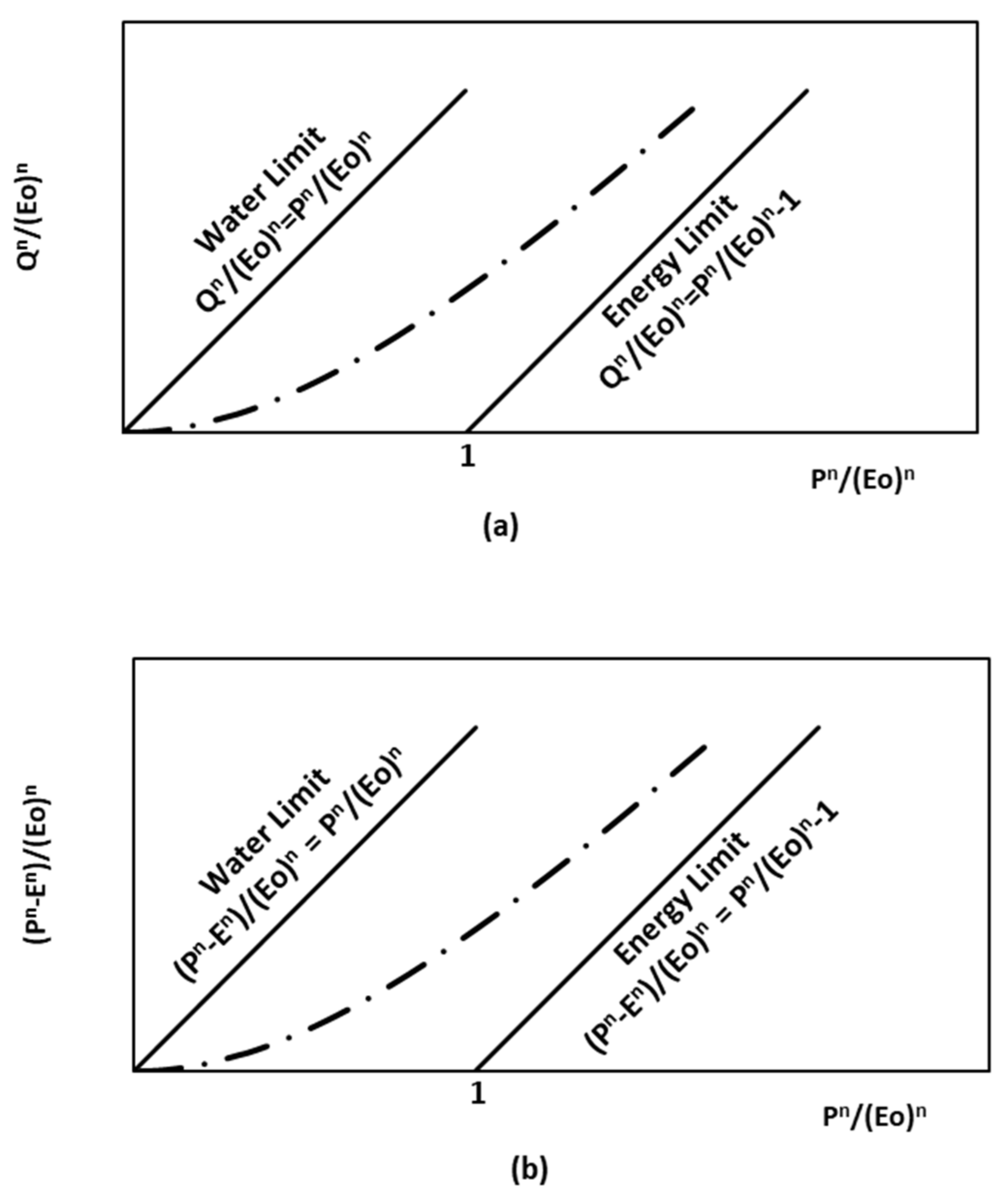
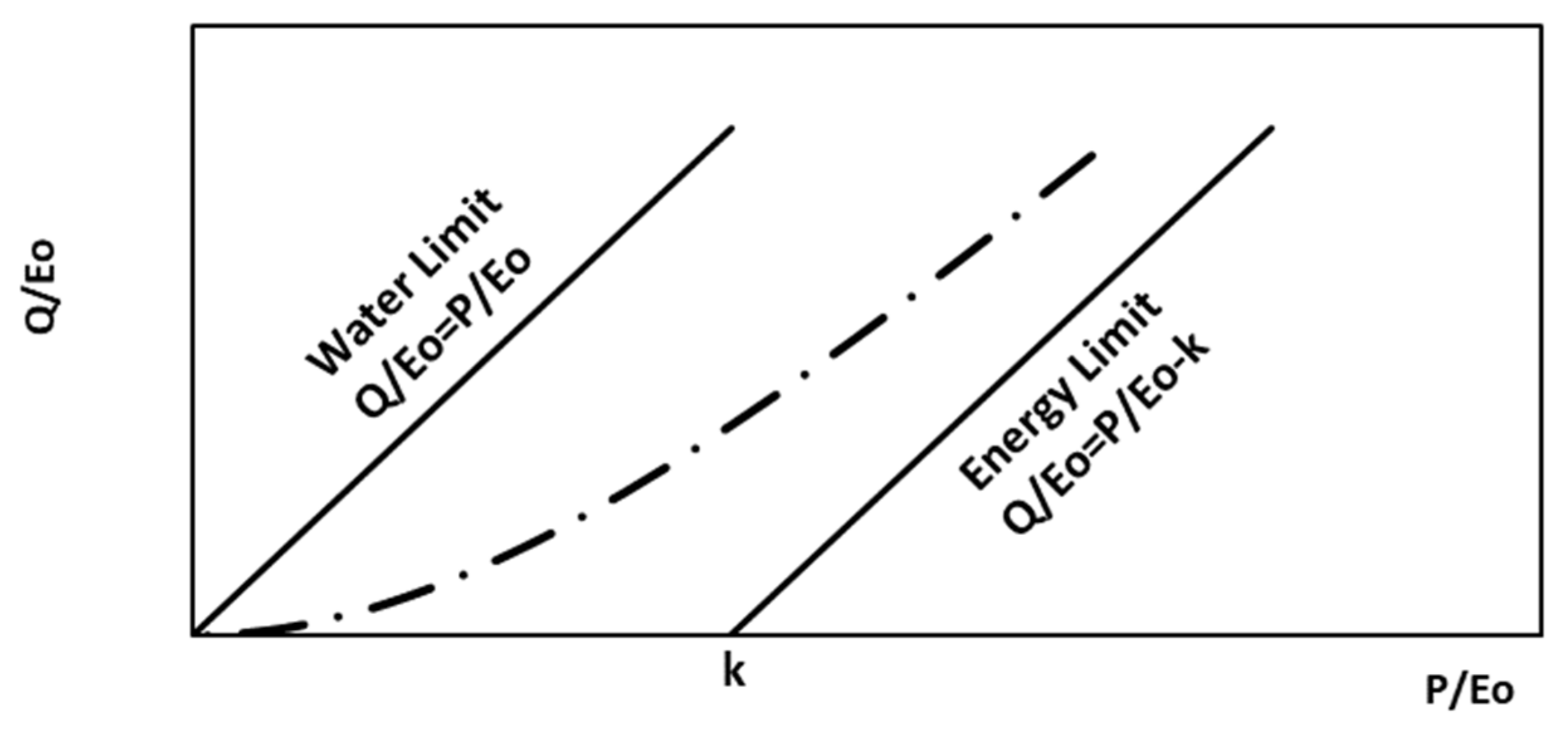
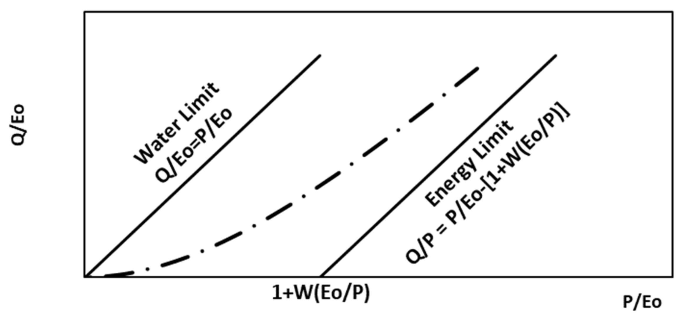
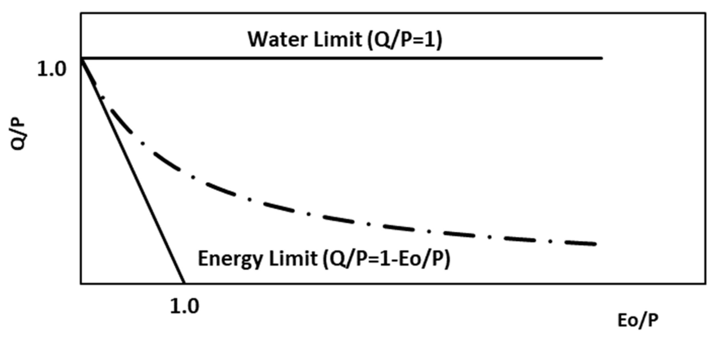
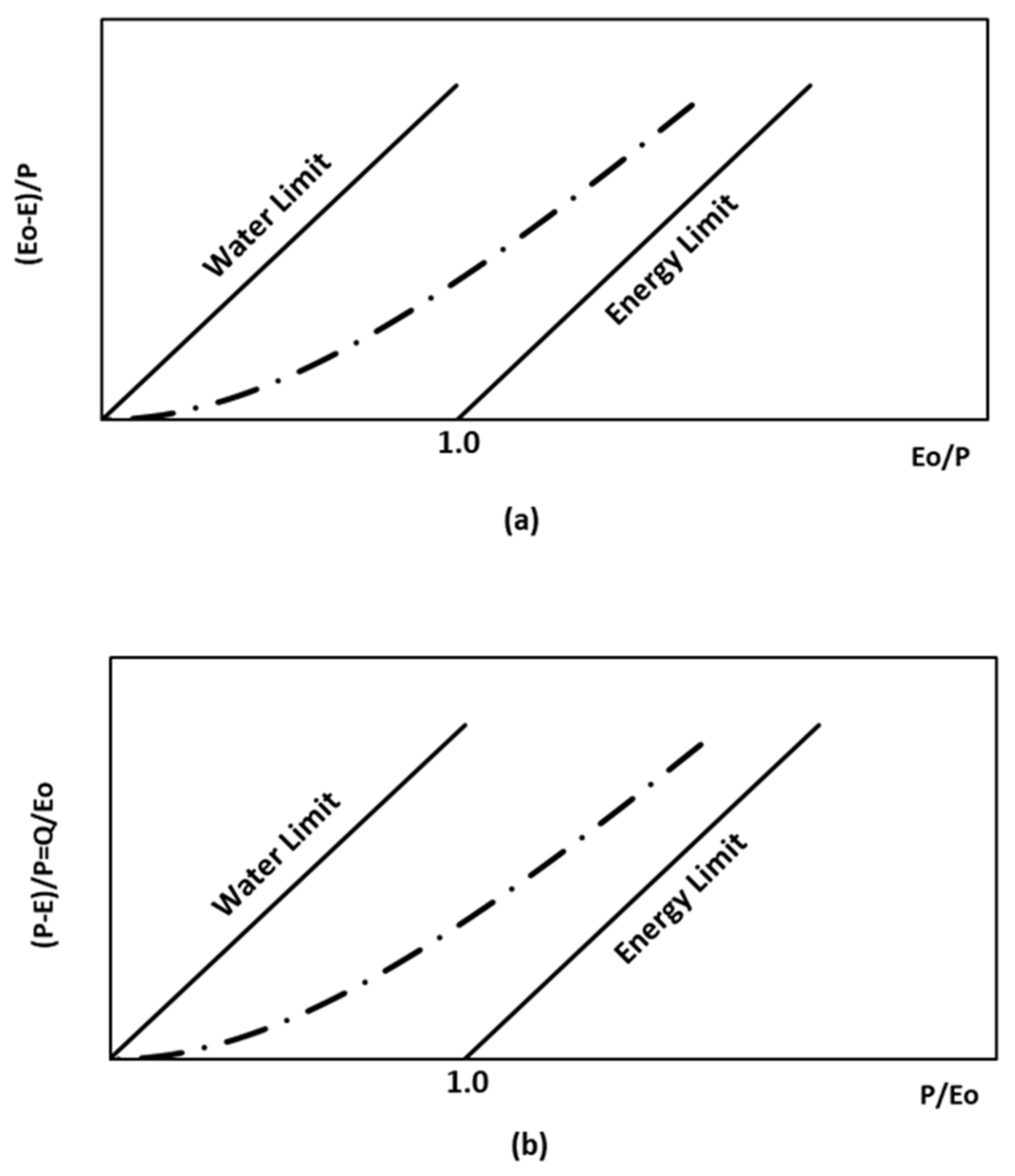
2.1. Budyko Hypothesis and Representation Diagrams

Citation [6] put forward two basic hypotheses. First, the following relationship holds under very humid (energy-limited) conditions:
E P E o P ,   a s   E o P 0
where Eo is potential evapotranspiration. The following relationship holds under very dry (water-limited) conditions:
E P 1 ,   a s   E o P
The Budyko hypotheses are illustrated in Figure 1a (Budyko diagram; [15]), showing a relationship that meets the limits established. Budyko hypothesized that precipitation is partitioned between runoff and evapotranspiration in the first-order, and it is determined by balance between available water (P) and available energy (Eo); that is:
E = f P , E o
Another Budyko type diagram is the relationship P/Eo versus E/Eo (Turc diagram); ref. [15] as shown in Figure 1b. The energy limit is given by:
E E o 1 ,   a s   P E O
and the water limit by:
E E o P E o ,   a s P E O 0
Although other Budyko-type diagrams [16] might be easier to interpret than the one shown in Figure 1c, this one allows a straightforward analysis of the P–Q relationship in hydrological terms [17,18]. In this diagram, a functional relationship shall meet the energy limit:
E E 0 = P Q E o 1 ,   a s   P E O
and water limit:
E E 0 = P Q E 0 0 , a s   P E O 0
As will be discussed below, the diagram in Figure 1c can be converted, without loss of generality, into a P–Q diagram to yield the classical visualization of the precipitation-runoff Equation (2).

2.2. Budyko-Type Functional Relationships

The Budyko-type functional relationships will be given for the spaces shown in Figure 1. If E/P is known, then Q/P can be estimated using Equation (2). For the space P/Eo − E/Eo, it is necessary to change E/P by E/Eo after changing Eo/P by P/Eo if the relationship obeys Budyko limits [15]. Citation [19] put forward the model Q/P = 1 − exp(s/P), where s is a parameter. Reference [20] suggested that s can be replaced by Eo;
E P = 1 e x p E 0 P
E E o = P E o 1 e x p E 0 P
Q P = e x p E 0 P
Citations [21,22] developed a simple model to account for the Schreiber relationship as an equilibrium solution of the precipitation-runoff chain through the use of two water reservoirs operating two different time scales: a fast stochastic one that feeds the second (slower) reservoir. Citation [20] proposed the functional relationships:
E P = E o P t a n h P E o
E E o = t a n h P E o
Q P = 1 E o P t a n h P E o
Citation [23] found that water balance in many catchments falls between the Schreiber and the Ol’dekop curves, and therefore proposed to use the geometric mean of the two relationships:
E P = t a n h P E o E o P 1 e x p E o P 1 / 2
E E o = t a n h P E o P E o 1 e x p E o P 1 / 2
Q P = 1 t a n h P E o E o P 1 e x p E o P 1 / 2
These models do not include any fitting parameter, and thus they seemingly lack the flexibility to allow for specific conditions (vegetation, topography, etc.) in the hydrological response of catchments. To address this issue, citations [24,25] proposed the general Equation (10a) by introducing a variable m coefficient into the Schreiber relation:
E P = 1 e x p m E o P
Citation [26] also included a fitting parameter m in the Equations (10) and (12) changing Eo by mEo. Several authors [10,27,28,29,30,31] proposed a single-parameter model:
E P = 1 1 + P E o n 1 / n
E E o = 1 1 + E o P n 1 / n
Q P = 1 1 1 + P E o n 1 / n
This model, hereafter referred to as the TMPHCY model, utilizes either specific n values or a single overall n fitting parameter. Proposed by [28], the formulation is based on the relationship:
1 E n 1 E o n = 1 P n
which yields Equation (14a) when solved in terms of E/P.
Citations [12,32] proposed the relationship, hereafter referred to as the SZ model:
E P = k E o P k E o P + 1
E E o = k P E o k P E o + 1
Q P = 1 k E o P k E o P + 1
Citation [33] developed the following relationship, hereafter referred to as the Z model:
E P = 1 + W E o P 1 + W E o P + P E o
E E o = P E o + W 1 + W E o P + P E o
Q P = 1 1 + W E o P 1 + W E o P + P E o
As pointed out by citations [10,12,32], the Z model violates the Budyko energy limit when W > 1.
Citation [34] developed the relationship, hereafter referred to as the WT model:
E P = 1 + E o P 1 + E o P 2 4 ε 2 ε E o P 1 / 2 2 ε 2 ε
E E o = 1 + P E o 1 + P E o 2 4 ε 2 ε P E o 1 / 2 2 ε 2 ε
Q P = 1 1 + E o P 1 + E o P 2 4 ε 2 ε E o P 1 / 2 2 ε 2 ε
Finally, citations [8,11,35] formulated the following relationship, hereafter referred the TFZ model:
E P = 1 + E o P 1 + E o P ω 1 / ω
E E O = 1 + P E o 1 + P E o ω 1 / ω
Q P = 1 + E o P ω 1 / ω E o P
Each of these models includes one fitting parameter (m, k, n, W, ε, ω) that confers on them some flexibility to be parameterized according to the conditions and properties of catchments, although the models establish no explicit relationships with such conditions. [26] proposed the use of parameter m (Eo → mEo) in addition to parameter n (TMPHCY model) and ω (TFZ model).
Relationships showing a Budyko-type behavior have been developed from various hydrological models. For instance, [36] used a stochastic model of soil moisture [37] to formulate a model that yields patterns similar to Budyko-type relationships. [38] used the four-parameter abcd model developed by [39]; they parameterized b as a function of climate and used a simplified model of the variation of P and Q [38] to estimate the parameter a. The resulting model shows Budyko-type patterns.
Citation [40] presented a multiscale (days, months, and years) hydrological model of the components of actual evapotranspiration, including evaporation related to water surfaces, to produce patterns similar to Budyko-type functional relationships. Citation [41] used hydrological and vegetation models to generate patterns similar to Budyko’s functional relationships based on the principle of maximum entropy production in catchments.

3. Derivation of Selected Budyko-Type Models

The Budyko-type models presented in the previous section were developed on empirical bases. The TMPHCY (Equation (14)) and TFZ (Equation (19)) models were developed by means of dimensional analysis and mathematical reasoning using the boundary conditions that had to be met (i.e., water and energy limits). The mathematical development of those models is relatively complex and involves solving a system of partial differential equations subject to boundary conditions.
Citation [12] developed an alternative to dimensional analysis through generating functions that meet the water and energy limits by simplifying the mathematical complexity involved in developing Budyko-type models. Citation [9] proposed a generalized methodology for the mathematical derivation of Budyko-type models, with the method used by [12] as a particular case of this unified method.
Citation [12] stated that the TMPHCY model is the best Budyko-type model currently available, including the TFZ model, although [42] state that there are no hydrologically-based reasons to select one model over the other. It is, therefore, worth analyzing the TMPHCY model in detail.

4. Budyko-Type Models in the P–Q Space

4.1. Model TMPHCY

Citation [31] proposed that, given the limits set by Budyko hypotheses, the function:
y = x 1 + x
meets the limits when x = P/Eo and y = (P-Q)/Eo = E/Eo (see [43] for further discussion). A generalized form of this function is:
y = x 1 + x n 1 / n
The empirical argumentation given by Turc consists of utilizing a mathematical function that meets the conditions required, but without justifying its foundations beyond the limits. As discussed below, meeting the Budyko limits is not a sufficient condition for a function to be a hydrologically sound model.
For analyzing the model TMPHCY we will first consider the case n = 1. According to Figure 1c, the water limit will be defined by:
Q E o = P E o Q P = 1
and the energy limit by:
Q P = P E o 1 = > P Q E 0 = 1
Figure 2 shows a Budyko-type diagram on the P-Q space, which is strictly equivalent to the space shown in Figure 1b, since Eo cancels out when used in terms of ratios and the water and energy limits are the same; nevertheless, that use of ratios implies spurious self-correlation [44] because Eo is in both ratios (a common variable), as shown by [17]; (see also [45]).
In the following, we will use classical Budyko diagrams for consistency in representations, but all are equivalent to a simple P-Q representation (but presented more data dispersion).
To develop a Budyko model, the hypothesis (proportionality hypothesis; [34]) that water (Equation (22)) and energy (Equation (23)) limits are equal is made:
Q P = P Q E 0
Substituting Q = P − E, then:
P E P = P P E E 0 = E E o
Solving this relationship for E/P:
E o P E = EP = > PE o EE o = EP
EE o + EP = E E o + P = PE o
and the final result is:
E P = E o E o + P = 1 1 + P E o
This equation is the TMPCHY model with n = 1 (Equation (14a)).
The derivation shown above implies that two parallel lines (same slope but different intercepts, see Figure 1c) should be equal to each other. This is a result of the arithmetic (proportionality; see [34]) hypothesis (1 = 1) of equating two relations with similar values (Equations (22) and (23)), as opposed to the notion of algebraically equating variables, which, by equating Q from Equations (22) and (23), would lead to:
P = P Eo
which shows that this is valid if and only if Eo = 0; that is, when both parallel lines have a common intercept. The crucial point of the above derivation is that the shape (curvature) of the function obtained has no basis beyond the hypothesis that both parallel lines are equal despite having different intercepts. Although the relationship thus derived mathematically meets the Budyko limits (partially), it lacks any hydrological foundation (proportionality hypothesis).
The same argument that was described by [46] is the basis for the Soil Conservation Service (SCS) runoff curve-number (CN) method the P-Q relationship at the scale of daily rainfall events ([47]; currently [48]), starting from the so-called proportionality hypothesis (Equation (24)), with Eo = S (storage capacity of the catchment); see Appendix A for a trigonometric derivation of the proportionality hypothesis and its generalization. Citations [18,26] used the SCS model in the Budyko context.
Citation [49] pointed out that Equation (14a) does not satisfy the physical limit associated with humid environments due to the unfeasibility of Eo/P = 0 when E/Eo → 1.
A Budyko-type model must satisfy Q/P = 1 when P → ∞. Equation (14a) (n = 1) satisfy Q/P → 1 when P → , but never reaches Q = P. The partial derivative of Equation (14a) (n = 1) is given by:
Q P = 1 1 1 + 1 E o P 2
where for P → ∞ it is not defined (undetermined).
To overcome this problem, it is possible to use an energy limit with a variable slope α using a line defined by Q/P = (αQ − P)/S. Under the proportionality hypothesis the following relation is obtained:
Q P = P E o + P
which partial derivative is given by:
Q P = P E o 2 + P E o 1 + P E o
The limit ∂Q/∂P = 0 is reached if P = 0 or Eo = ∞.
Under the condition ∂Q/∂P = 1 the value of α is:
= 1 2 E o P + 1 4 + E o P 1 2
where if Eo/P → 0 then α → 1 and original Equation (14a) (n = 1) is recovered.
Citation [50] developed a similar approach (Equation (25)) under the context of the CN-SCS method.
The generalized form (Equation (14)) for any n is obtained when Eo is substituted by (Eo)n, P by Pn, and Q by Qn.Figure 3a shows the situation when the variables are raised to the n-th power.
From Figure 3a the water limit is:
Q n E o n = P n E o n = > Q n P n = 1
and the energy limit is:
Q n E o n = P n E o n 1 = > P n Q n E o n = 1
Under the proportionality hypothesis then:
Q n P n = P n Q n E o n
Solving for Q/P we obtain:
Q P = P E o n + P n 1 / n
Using Equation (2), then:
E P = E o n + P n 1 / n P E o n + P n 1 / n
This equation can be simplified under the hypothesis:
P + E o = P n + E o n 1 / n
1 + E o P = 1 + E o P n 1 / n
which meets water and energy limits Eo/P → 0 and Eo/P → , respectively. Substituting this last relation in Equation (27), we obtain:
E P = E o E o n + P n 1 / n = 1 1 + P E o n 1 / n
which is the TMPHCY model (Equation (14a)).
A direct alternative to develop the TMPHCY model is to use limits of Figure 3b. As before, the proportionality hypothesis is given by:
P n E n P n = P n E o n P n E n E o n
Solving for E/P we obtain:
E P = E o E o n + P n 1 / n = 1 1 + P E o n 1 / n
which is the TMPHCY model (Equation (14a)).

4.2. Model SZ

In Figure 4 the water limit is given by:
Q E o = P E o = > Q P = 1
and the energy limit by:
Q P = P E o k = > P Q kE 0 = 1
under the proportionality hypothesis:
Q P = P Q kE 0
Using Q = P − E and solving for E/P, we obtain:
E P = kE o P + kE 0 = k Eo P k Eo P + 1
which is the SZ model (Equation (16a)).

4.3. Model Z

Figure 5 shows the water limit for this model:
Q E o = P E o = > Q P = 1
and the energy limit by:
Q E 0 = P E o 1 + W E 0 P = > P Q E 0 + W E o 2 P = 1
The proportionality hypothesis is established as:
Q P = P Q E 0 + W E o 2 P
Substituting Q = P − E and solving for E/P:
E P = E o + W E o 2 P P + E o + W E o 2 P = 1 + W Eo P 1 + W Eo P + P Eo
which is the Z model (Equation (17a)).

4.4. Model WT

Citation [34] develop their model using the generalized proportionality hypothesis. In this case, the TMPHCY model is obtained by simply substituting P by Pe (= P − Ei) in Equation (14a) with n = 1, where Pe is effective precipitation. In the SCS (today the National Resources Conservation Service or NRCS) curve number, Pe = P − Ia [46], where Ia is the initial abstraction (storage in troughs, interception by vegetation, etc.). Over an annual period, some of the precipitation (Pi = Ei) is not expected to contribute to runoff (initial abstractions from rainfall events) and, thus, this consideration holds true. Citation [51] proposed this modification to the TMPHCY model, and [52] did the same for the TFZ model.
According to Figure 6, the water limit is:
Q E o = P E i E o = > Q P E i = 1
and the energy limit by:
Q E 0 = P E i E o E o E i E i = > P E i Q E 0 E i = 1
Under the proportionality (generalized) hypothesis and using Q =P − E we obtain:
P E P E i = P E i P E E 0 E i = E E i E 0 E i
Citation [53] called this relationship the generalized proportionality hypothesis (see Appendix A), the same proportionality hypothesis but with an intercept different from zero. Citations [54,55] utilized this relation with the two-phase concepts (precipitation and wetting) of [56].
Dividing the numerator and denominator by P in both sides of Equation (28):
1 E P 1 E i P = E P E i P E 0 P E i P
Using ε = Ei/Eo, then substituting Ei = εE in the previous equation:
1 E P 1 ϵ E P = E P ϵ E P E 0 P ϵ E P
Solving the equation for E/P, we obtain:
ϵ 2 ϵ E P 2 1 + E o P E P + E o P = 0
This equation can be solved considering that E/P is positive and less than 1:
E P = 1 + E o P 1 + E o P 2 4 ε 2 ε E o P 1 / 2 2 ε 2 ε
which is the WT model (Equation (18a)).

4.5. Non Proportionality Hypothesis Models

One way to analyze differences between proportionality hypothesis related models (e.g., TMPHCY) is using Eo/P − Q/P space [16], Figure 7. This diagram shows that the water limit is defined by:
Q P 1 ,   a s   E o P 0
and the energy limit by:
Q P 0 ,   a s   E o P
First, the Q/P TMPHCY model (Equation (14c)) must be converted in terms of P/Eo as Equation (19c) of the TFZ model:
Q P = 1 1 1 + 1 P / E o n 1 / n
Equation (31) is not defined for P/Eo = 0 and it is not a valid model for this limit (water). In this limit, the TFZ model gives Q/P = 1 (water limit).
According to [10], the parameters n and ω are linearly related:
ω n + 0.72
although [12,42] show that this relation is imprecise. Both models are generated using different hypotheses, and it is expected that results differ.
With regard to the Schreiber model (Equation (10c)) and the [20], both models satisfy the water limit, but not the extreme energy limit (horizontal and oblique line in Figure 2) as discussed below.
Another way to visualize differences among the proportionality and no proportionality hypothesis models is using the ∂E/∂P function of [57]:
E P = 1 E E o p
If p = 1 then the Schreiber model is generated through the integration of Equation (46) and if p = 2 the Ol’dekop model is obtained. Citation [29]; introduces the following relation:
E P = 1 E E o n 1 + 1 n
Integrating this equation, we obtain the TMPHCY model.
Regarding the TFZ model, ∂E/∂P is given by:
E P = 1 1 + E o P w 1 w 1 E o P w 1
Equations (32) and (34) have a different mathematical structure than Equation (33).
Citation [8], see [11,42], derived TFZ model using the variables (Eo − E)/P and (P − E)/Eo (= Q/Eo). Using these variables, the water and energy limits can be stablished as shown in Figure 8.
The TFZ model cannot be derived using the proportionality hypothesis applied to the spaces shown in Figure 8, in particular the space of Figure 8b used in the derivation of model TMPHCY.

5. An Expolinear Model of the P–Q Relationship

One of the problems faced by empirical models (Equations (10c), (11c) and (12c)) is that they cannot approach the extreme energy limit shown in Figure 2 (both horizontal and inclined line). In order to comply with this objective, the exponential model (Equation (10c)) could be extended to an expolinear model [46]. Something similar could be done for the tanh model (Equation (11c)).
The expolinear model could be developed if the relation between P and Q is considered as composed by two parts:
Exponential   Growth :   Q P = m Q ,   Q = Q 0 e x p m P
Linear   Growth :   Q P = C ,   Q = C P E 0
In the transition between the exponential growth to the lineal one, the rates of change have to be the same (mQ = C). The solution to both types of growth is an expolinear model (see [58]):
Q = C m l n ( 1 + e x p m P E 0
where the transition point (PT, QT) from exponential to linear is defined by:
Q P = P T = C m = Q T
P T = E 0 + 0.541 m
The model in Equation (37) fulfills the Budyko extreme limits [59]) and only requires one parameter (m), because C = 1 [60] is the energy limit.

6. Discussion

Arguably, under the perspective of the equifinality thesis [61], the dimensional analysis of [10] in developing the TMPHCY model could be considered as a possible alternative route to find the same solution as the proportionality hypothesis; however, the mathematical evidence (flaws) shows that the dimensional approach used by [10] is equivalent to the hypothesis.
The derivations herein presented illustrate a universal concept in developing hydrological relationships from the daily to the annual scale [12], which is a hypothesis (proportionality) that has no hydrological bases beyond meeting the limit conditions, making no contributions to the knowledge of what happens between the limits (partially satisfied).
Same claims as [12] can be made using daily hydrological models similar to the Budyko-type analyzed. The Schreiber model, with the modification of Ol’dekop, is similar to the model proposed by [62], using natural logarithms:
Q P = 1 exp bP
where b is a fitting parameter (b = 1/Eo in the context of Budyko models). Note that this equation is put in terms of P, not 1/P as Equation (10c). Nevertheless, this model is equivalent to the Schreiber model inverting numerator and denominator in the previous equation.
Another model used in a daily basis was proposed by [63]:
Q P = 1 f P tan h P f
where f is daily loss (f = Eo in the context of Budyko models).
Finally, a similar model to the TFZ was proposed by [64]:
Q P = 1 + d P t 1 / q d P
where d is daily water deficiency (d = Eo in the context of Budyko models) and q is a fitting parameter.
The use of mathematical tools is essential for establishing hydrological relationships based on the principle of mass and energy balance coupled with the use of hydrological—not merely mathematical—reasoning. Emphasizing mathematical properties that support hydrological “knowledge” leads to circular arguments based on empirically grounded hypotheses such as Budyko’s limits. The boundary conditions set limits that cannot be surpassed, but they do not provide specific information on what happens in between those boundaries. From the standpoint of the Darwinian approach [5], the limits define the minimum requirements that any hydrological development should meet to be used to reduce the complexity of hydrological models.
The use of hydrologically intuitive spaces, such as P − Q, adds perspective to the hypotheses implicit in the formulation of some Budyko-type models, in addition to incorporating variables hydrologically associated to catchments, such as the initial abstraction and the storage capacity of soil (and similar definitions), with no need to resort to the potential evapotranspiration concept. However, unlike initial abstraction and storage capacity, potential evapotranspiration can be readily estimated, allowing models to become operational.

7. Conclusions

This paper analyses different Budyko type models in a unique representation that shows that all of the models use the proportionality hypothesis, with different formulations, as a base for developments. If the proportionality (and the generalized version, a simple change of the origin of coordinates) is not valid (valid only in trigonometrical terms, not in algebraic ones), then all models analyzed are not mathematically correct.
A new model is proposed to satisfy the imposed conditions, in addition to the model developed by Fu and others, depending on only one parameter. The introduced model has another parameter that can be allowed to change when precipitation is not enough to meet the energy limit.
As a conclusion from this review, the authors call for the hydrological community to not disregard their intuition, but rather visualize—beyond the mathematical complexities—the essence of the hypotheses being proposed and avoid the temptation to assume that mathematical proofs are sufficient to make a theory correct. This step is necessary for new developments in hydrology avoiding to do science with unverified assumptions [65].

Author Contributions

Conceptualization, writing—original draft, F.P.P.; formal analysis, F.P.P. and J.G.P.; writing—review & editing V.S.A., A.S.V.R. and M.A.B.G. All authors have read and agreed to the published version of the manuscript.

Funding

This research received no external funding.

Data Availability Statement

Not applicable.

Conflicts of Interest

The funders had no role in the design of the study; in the collection, analyses, or interpretation of data; in the writing of the manuscript, or in the decision to publish the results.

Nomenclature

SymbolUnitDescription
PmmPrecipitation
EmmActual evapotranspiration. The E symbol in hydrology is commonly used for Evaporation, but we change it in line with common notations in Budyko type models
QmmRunoff
E0mmPotential evapotranspiration. Symbol changed as used in common hydrology practice
m, k, n, W, ε, ω, α, b, f, d-Fitting parameters of the Budyko type models

Appendix A

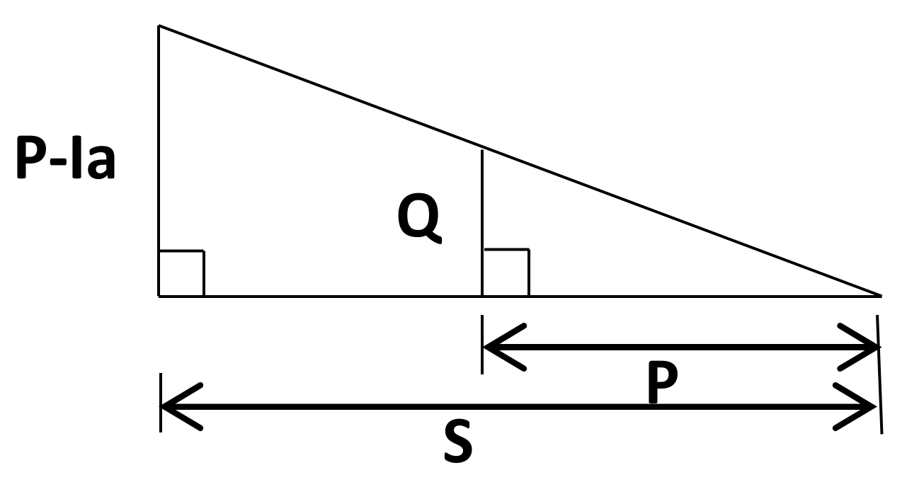
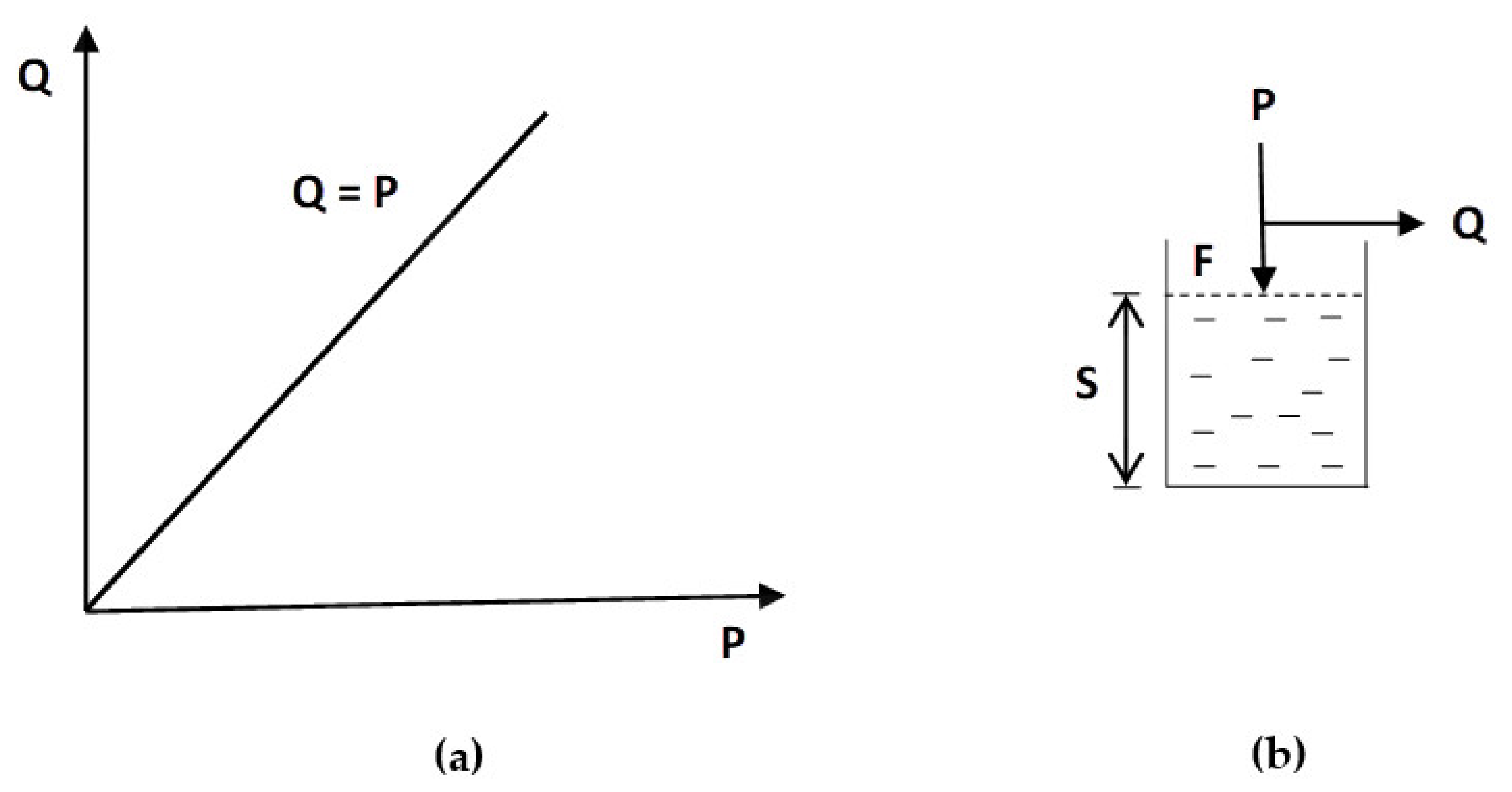
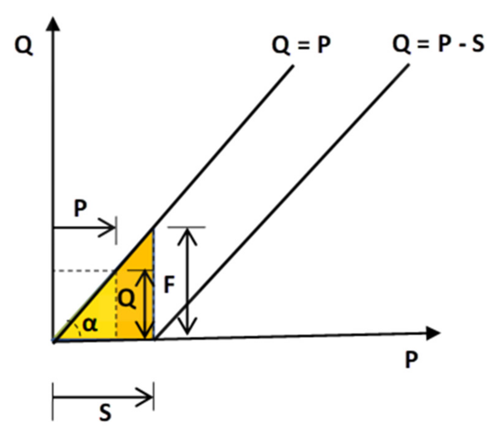
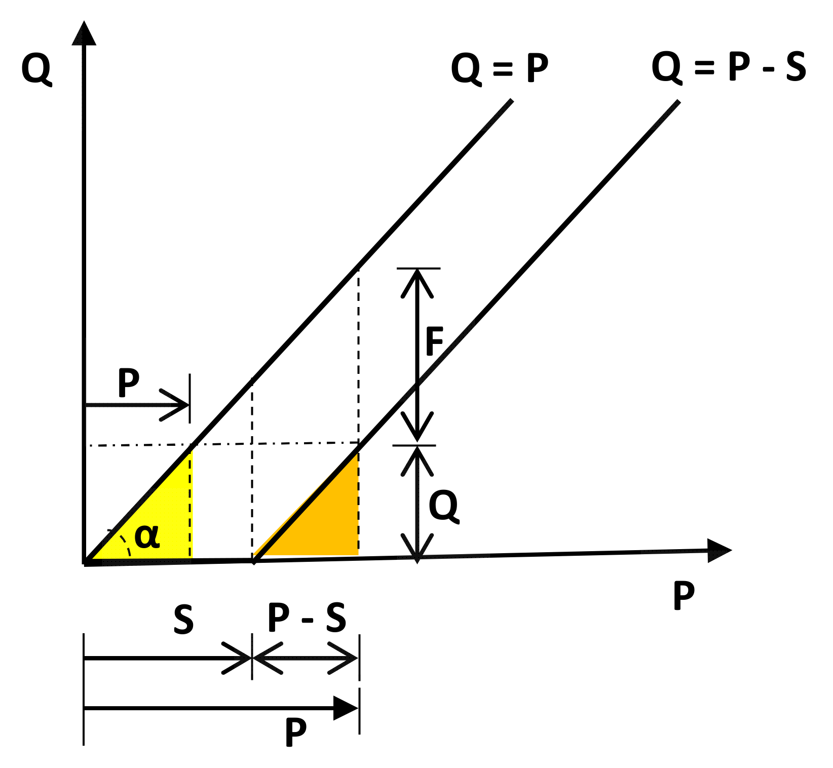
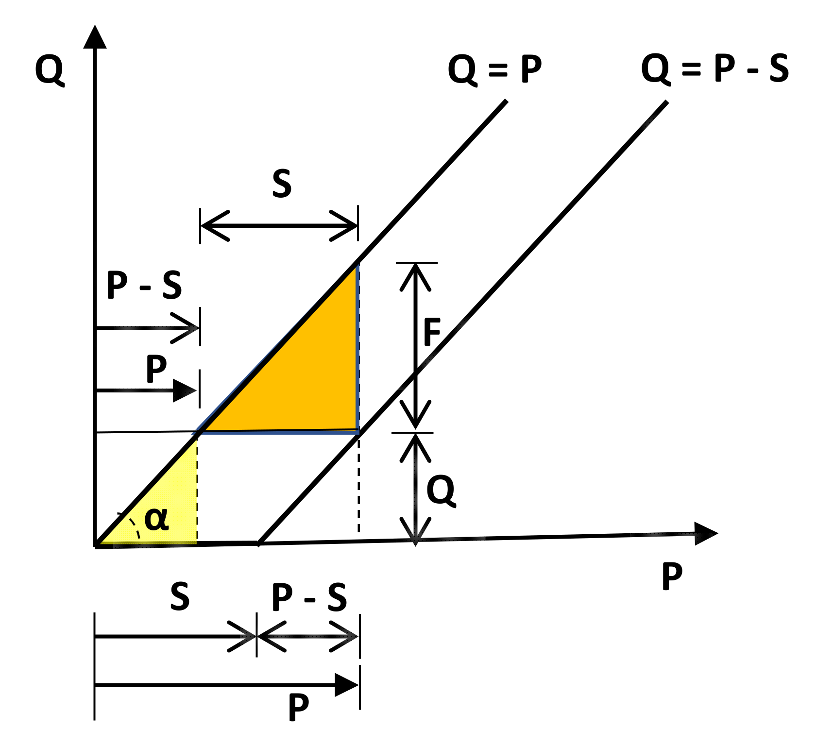
Appendix A.1. Proportionality Hypothesis of the CN-SCS Method

The discussion of the proportionality hypothesis of the SCS/NRCS curve number method generally starts from the identity relationship generated by the equation and sometimes sketches its interpretation using the space-time [66], which is not clear to understand its implications. In simple terms, without context, it is relatively normal (e.g., [67]) to use the next diagram (Figure A1) to explain the hypothesis.
Figure A1. The developments shown are strictly similar for the case of a Budyko P − Q dia-gram.
Water 14 03315 g0a1
The developments shown are strictly similar for the case of a Budyko P − Q diagram, where in the following S is storage potential capacity (=Eo), Ia is initial abstraction (=Pi or Ei, initial precipitation or evapotranspiration not contributing to runoff), and F is cumulative infiltration (=E). The water balance is given by P = F + Q.

Appendix A.2. P-Q Space Limits

The water limit is defined in Figure A2a, which uses a simple model of a saturated bucket (Figure A2b), where all precipitation (P) produces runoff (Q).
Figure A2. (a) Water limit in the P-Q space and (b) simple model of a single saturated bucket, with F = 0.
Water 14 03315 g0a2
The soil storage limit (energy limit) is shown in Figure A3a, where the soil water storage is empty at the beginning and only when it is full (F = S) does runoff (Q) begin. The above represents a simple model of a single empty bucket (Figure A3b).
Figure A3. (a) Water storage limit (energy limit) in P − Q space and (b) simple model of a single empty bucket, with F > 0.
Water 14 03315 g0a3

Appendix A.3. Case Ia = 0

The case of Ia = 0 and analysis concerning the line Q = P, Figure A4, up to the limit P = S defines the trigonometric identity of the two shown triangles (α = 45°):
tan = 1 = Q P = F S
Figure A4. Case of Ia = 0 for the analysis concerning the Q = P line.
Water 14 03315 g0a4
Using the Equation (A1), the CN-SCS model (F = P − Q) can be developed:
Q = P 2 P + S
In general, for the condition Q = P (S = 0, so Q = P), the CN-SCS method is strictly valid, but S is not required, nor used.
In the case of using the two straight lines (Q = P and Q = P − S) as a reference (Figure A5), the trigonometric equality of the two equal triangles shown gives:
tan = 1 = Q P = Q P S
It is important to note that although it is a mathematically valid trigonometric identity, in algebraic terms it is valid if and only if S = 0 (line Q = P as a reference) in P = P − S.
Figure A5. Case of Ia = 0 for the analysis concerning the line Q = P and Q = P − S, equal triangles.
Water 14 03315 g0a5
Additionally, in case of using the two straight lines (Q = P y Q = P − S) as a reference, in Figure A6, the trigonometric equality of the two similar triangles shown gives:
tan = 1 = Q P = F S
Therefore, with F = P − Q, it generates the Equation (A2) of the CN-SCS method.
Figure A6. Case of Ia = 0 for the analysis concerning the line Q = P and Q = P − S, similar triangles.
Water 14 03315 g0a6
In Figure A6 the minor triangle (yellow filling) has the horizontal side (P) defined with respect to the line Q = P and the same side (P − S) defined with respect to the line Q = P − S. Thus, using the line Q = P − S as a reference it is obtained:
tan = 1 = Q P S = F S
From the Equations (A4) and (A5), it is obtained:
tan = 1 = Q P S = Q P
which is valid if and only if S = 0, using the line Q = P as reference.

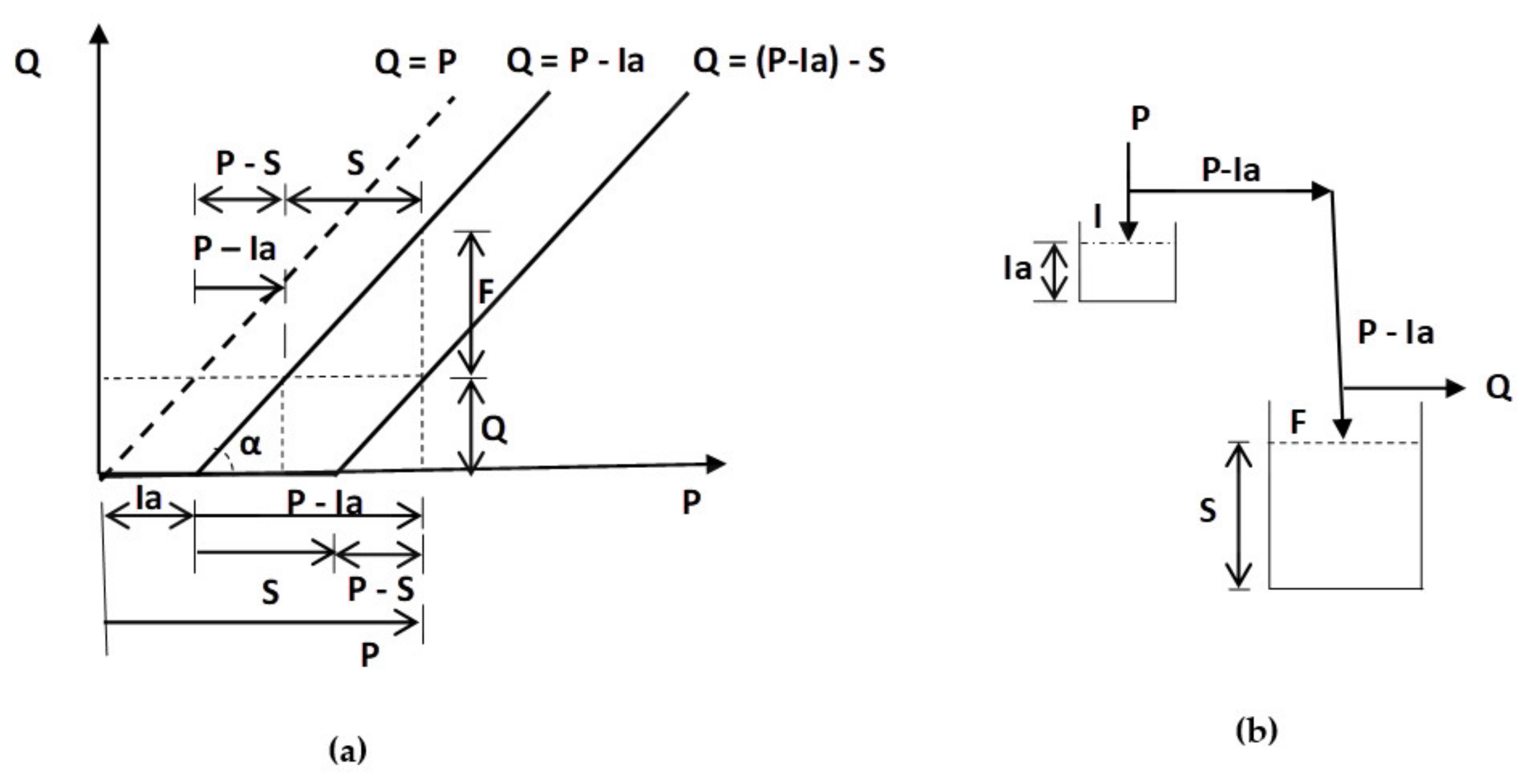
Appendix A.4. Case Ia > 0 and Different Origins of P and S

For the case of Ia > 0, for runoff to occur, this reservoir must be filled first (Figure A7b) and, depending on the state of the storage S, it will run off immediately or after saturation (Figure A7b). Figure 7a shows the relations of the P-Q space. Similar to those in Figure A6, but for the situation where S is defined as additional to Ia and P at the origin. In this situation, the previous discussion is valid only with the change from P to (P − Ia).
Figure A7. Case of Ia > 0, with S and P with different origins (a) and simple two-bucket model (b).
Water 14 03315 g0a7

Appendix A.5. Case Ia > 0 and Equal Origins of P and S

The case of Ia > 0 and equal origins of P and S, also known as generalized proportionality hypothesis [53], is shown in Figure A8, where the definitions of the P-Q space are shown in Figure A8a and the simple single bucket model is shown in Figure A8b.
Figure A8. (a) Case of Ia > 0, with S and P with equal origins and (b) a simple model of one bucket with two reservoirs.
Water 14 03315 g0a8
The situation of common origins of S and P only requires changing these variables to (S − Ia) and (P− Ia) to reach the same conclusions as the previous cases analyzed.

Appendix A.6. General Discussion

The analyses shown define that the proportionality hypothesis (and its generalization) is correct as a trigonometric identity, but not valid in algebraic terms for use in P-Q models. The trigonometric identity is equivalent to an algebraic one only when S = 0, meaning when only the limit Q = P is used. In other words, the two straight lines (slopes of 45 °) are equal if and only if they have a common origin (S = 0). In this perspective, the hypothesis of Budyko-type models based on proportionality implies the equality of the two limits (water and energy), which is not a valid hypothesis in algebraic terms. The situation of using the straight-line Q = P − S as a reference cannot be defined, since in the limit when P → the slope of this line (tan 45° = 1) can never be reached, implying the existence of infinite storage in the basin [68].

Appendix A.7. Historical Context

Documentation of the development of the CN-SCS method is relatively poor, with some attempts to present its history [69]. Officially, Mockus presented the method in 1972 [70] in a format similar to that used today.
A letter from the author of the CN-SCS to Orrin Ferris [71] states that the simple hypothesis used was:
F S 1   a n d   Q P 1 ,   w h e n   P
Therefore, the equality defined by Equation (A1) was established.
The argument to justify the hypothesis was [71] “on the grounds that it produces rainfall-runoff curves of a type found in natural watersheds” or, as [72] established “whether we accept or reject Equation (A1) for practical use depends on its agreement with watershed data”. This utilitarian argument of the CN-SCS method was used to justify it as “factually true” [73]. To the question of whether it is algebraically true, no answer was obtained [73].
It is interesting to note that [73,74] define that the CN-SCS equation was not derived (e.g., there was no hypothesis initially) but was discovered after trying other equations, and its selection was made because it was the least complex. In statistical terms, the relation Q/P = (P − Q)/S (or variants) was used in the analysis using the available data [73,74], obtaining good results. The good correlation obtained by using this relation is due to a spurious correlation [44], since the variables P and Q are on both sides of the equation.
Finally, considering the situation that the P-Q relation of the NC-SCS was discovered and not derived (it was done later by using the “proportionality hypothesis”), the authors agree with [66] regarding the proportionality hypothesis (Equation A1) “This assumption seems to be quite arbitrary and has no theoretical or empirical justification…”.

References

  1. Klemeš, V. Conceptualization and scale in hydrology. J. Hydrol. 1983, 65, 1–23. [Google Scholar] [CrossRef]
  2. Sivapalan, M.; Blöschl, G.; Zhang, L.; Vertessy, R. Downward approach to hydrological prediction. Hydrol. Process. 2003, 17, 2101–2111. [Google Scholar] [CrossRef]
  3. Littlewood, I.G.; Croke, B.F.W.; Jakeman, A.J.; Sivapalan, M. The role of ‘top-down’ modelling for Prediction in Ungauged Basins (PUB). Hydrol. Process. 2003, 17, 1673–1679. [Google Scholar] [CrossRef]
  4. Arnold, J.G.; Srinivasan, R.; Muttiah, R.S.; Williams, J.R. Large area hydrologic modeling and assessment part I: Model Development. J. Am. Water Resour. Assoc. 1998, 34, 73–89. [Google Scholar] [CrossRef]
  5. Hartman, C.; Troch, P.A. What makes Darwinian hydrology “Darwinian”? Asking a different kind of question about landscapes. Hydrol. Earth Syst. Sci. 2014, 18, 417–433. [Google Scholar] [CrossRef] [Green Version]
  6. Budyko, M.I. The Heat Balance of the Earth’s Surface; National Weather Service, U.S. Department of Commerce: Washington, DC, USA, 1958; pp. 144–155. [Google Scholar]
  7. Wang, C.; Wang, S.; Fu, B. Advances in hydrological modelling with the Budyko framework: A review. Prog. Phys. Geogr. 2016, 40, 409–430. [Google Scholar] [CrossRef]
  8. Fu, B.P. On the calculation of the evaporation from land surface. Sci. Atmos. Sin. 1981, 51, 23–31. Available online: https://en.cnki.com.cn/Article_en/CJFDTOTAL-DQXK198101002.htm (accessed on 13 February 2021). (In Chinese).
  9. Sposito, G. Understanding the Budyko equation. Water 2017, 9, 236. [Google Scholar] [CrossRef] [Green Version]
  10. Yang, H.; Yang, D.; Lei, Z.; Sun, F. New analytical derivation of the mean annual water-energy balance equation. Water Resour. Res. 2008, 44, W03410. [Google Scholar] [CrossRef]
  11. Zhang, L.; Hickel, K.; Dawes, W.R.; Chiew, F.H.S.; Western, A.W.; Briggs, P.R. A rational function approach for estimating mean annual evapotranspiration. Water Resour. Res. 2004, 40, W02502. [Google Scholar] [CrossRef]
  12. Zhou, S.; Yu, B.; Huang, Y.; Wang, G. The complementary relationship and generation of the Budyko functions. Geophys. Res. Lett. 2015, 42, 1781–1790. [Google Scholar] [CrossRef]
  13. Klemeš, V. Dilettantism in hydrology: Transition or destiny? Water Resour. Res. 1986, 22, 177S–188S. [Google Scholar] [CrossRef]
  14. Dooge, J.C.I. Hydrological models and climate change. J. Geophys. Res. 1992, 97, 2677–2686. [Google Scholar] [CrossRef]
  15. Lhomme, J.P.; Moussa, R. Matching the Budyko functions with the complementary evaporation relationship: Consequences for the drying power of the air and the Priestley-Taylor coefficient. Hydrol. Earth Syst. Sci. 2016, 20, 4857–4865. [Google Scholar] [CrossRef]
  16. Andréassian, V.; Perrin, C. On the ambiguous interpretation of the Turc-Budyko nondimensional graph. Water Resour. Res. 2012, 48, W10601. [Google Scholar] [CrossRef]
  17. Carmona, A.M.; Sivapalan, M.; Yaeger, M.A.; Poveda, G. Regional patterns of interannual variability of catchment water balances across the continental U.S.: A Budyko framework. Water Resour. Res. 2014, 50, 9177–9193. [Google Scholar] [CrossRef]
  18. Mouelhi, S. Vers una Chaîne Coherente de Modelès Pluie-Débit Conceptuels Globaux pas Temps Pluriannuel, Annuel, Mensual et Journalier. Thèse de Doctorat, École Nationale du Génie Rural, des Eaux et Forêts, Paris, France, 2003. Available online: https://pastel.archives-ouvertes.fr/tel-00005696/document (accessed on 19 February 2021).
  19. Schreiber, P. Über die Beziehungen zwischen dem Niederschlag und der Wasserführung der Flüsse in Mitteleuropa. Meteorolog. Z. 1904, 21, 441–452. [Google Scholar]
  20. Ol’dekop, E.M. On evaporation from the surface of river basins. T. Meteorol. Obs. 1911, 4, 200. (In Russian) [Google Scholar]
  21. Fraedrich, K. A parsimonious stochastic water reservoir: Schreiber´s 1904 equation. J. Hydrometeorol. 2010, 11, 575–578. [Google Scholar] [CrossRef]
  22. Fraedrich, K.; Sielmann, F. An equation of state for land surface climates. Int. J. Bifurc. Chaos 2011, 21, 3577–3587. [Google Scholar] [CrossRef]
  23. Budyko, M.I. Climate and Life, 1st ed.; Academic Press: Orlando, FL, USA, 1974; p. 508. [Google Scholar]
  24. Oudin, L.; Andréassian, V.; Lerat, J.; Michel, C. Has land cover a significant impact on mean annual streamflow? An international assessment using 1508 catchments. J. Hydrol. 2008, 357, 303–316. [Google Scholar] [CrossRef]
  25. Paz, F.; Marín, M.I.; López, E.; Zarco, A.; Bolaños, M.A.; Oropeza, J.L.; Martínez, M.; Palacios, E.; Rubiños, E. Elements for developing an operational hydrology with remote sensing: Soil-vegetation mixture. Ing. Hidraul. Mex. 2009, 24, 69–80. (In Spanish) [Google Scholar]
  26. Mouelhi, S. Existe-t-il une relation entre les modelès pluie-débit au pas de temps pluriannual? Rev. Sci. Eau 2011, 24, 193–206. [Google Scholar] [CrossRef] [Green Version]
  27. Choudhury, B.J. Evaluation of an empirical equation for annual evaporation using field observations and results from a biophysical model. J. Hydrol. 1999, 216, 99–110. [Google Scholar] [CrossRef]
  28. Hsuen-Chun, Y. A composite method for estimating annual actual evapotranspiration. Hydrol. Sci. J. 1988, 33, 345–356. [Google Scholar] [CrossRef]
  29. Mezentsev, V.S. More on the calculation of average total evaporation. Meteorol. Gidrol. 1955, 5, 24–26. (In Russian) [Google Scholar]
  30. Pike, J.G. The estimation of annual runoff from meteorological data in a tropical climate. J. Hydrol. 1964, 2, 116–123. [Google Scholar] [CrossRef]
  31. Turc, L. Le bilan D’eau Des Sols. Relation Entre la Précipitation, L’évaporation et L’écoulement. Ann. Agron. 1954, 5, 491–569. Available online: https://www.persee.fr/docAsPDF/jhydr_0000-0001_1955_act_3_1_3278.pdf (accessed on 26 February 2021).
  32. Sharif, H.O.; Crow, W.; Miller, N.L.; Wood, E.F. Multidecadal high-resolution hydrological modeling of the Arkansas-Red River basin. J. Hydrometeorol. 2007, 8, 1111–1127. [Google Scholar] [CrossRef]
  33. Zhang, L.; Dawes, W.R.; Walker, G.R. Response of mean annual evapotranspiration to vegetation changes at catchment scale. Water Resour. Res. 2001, 37, 701–708. [Google Scholar] [CrossRef]
  34. Wang, D.; Tang, Y. A one parameter Budyko model for water balance captures emergent behaviour in Darwinian hydrologic models. Geophys. Res. Lett. 2014, 41, 4567–4577. [Google Scholar] [CrossRef] [Green Version]
  35. Tixeront, J. Prévision des apports des cours d’eau. In Proceedings of the Symposium Eau de Surface Tenu à L’occasion de l’Assemblée Générale de Berkeley de L’U. G.G. I., Berkeley, CA, USA, 19–31 August 1963. [Google Scholar]
  36. Porporato, A.; Daly, E.; Rodriguez-Iturbe, I. Soil water balance and ecosystem response to climate change. Am. Nat. 2004, 164, 625–632. [Google Scholar] [CrossRef] [PubMed]
  37. Rodriguez-Iturbe, I.; Porporato, A.; Ridolfi, L.; Isham, V.; Coxi, D.R. Probabilistic modelling of water balance at a point: The role of climate, soil and vegetation. Proc. Royal Soc. Lond. A 1999, 455, 3789–3805. [Google Scholar] [CrossRef]
  38. Sankarasubramanian, A.; Vogel, R.M. Annual hydroclimatology of the United States. Water Resour. Res. 2002, 38, 1083. [Google Scholar] [CrossRef]
  39. Fernandez, W.; Vogel, R.M.; Sankarasubramanian, A. Regional calibration of a watershed model. Hydrol. Sci. J. 2000, 45, 689–707. [Google Scholar] [CrossRef]
  40. Gerrits, A.M.J.; Savenije, H.H.G.; Veling, E.J.M.; Pfister, L. Analytical derivation of the Budyko curve based on rainfall characteristics and a simple evaporation model. Water Resour. Res. 2009, 45, W04403. [Google Scholar] [CrossRef]
  41. Porada, P.; Kleidon, A.; Schymanski, S.J. Entropy production of soil hydrological processes and its maximization. Earth Syst. Dynam. 2011, 2, 179–190. [Google Scholar] [CrossRef] [Green Version]
  42. Andréassian, V.; Sari, T. Technical note: On the puzzling similarity of two water balance formulas—Turc-Mezentsev vs Tixeront-Fu. Hydrol. Earth Syst. Sci. 2019, 23, 2339–2350. [Google Scholar] [CrossRef] [Green Version]
  43. Lebecherel, L.; Andréassian, V.; Perrin, C. On regionalizing the Turc-Mezentsev water balance formula. Water Resour. Res. 2013, 49, 7508–7517. [Google Scholar] [CrossRef]
  44. Kenney, B.C. Beware of spurious self-correlations! Water Resour. Res. 1982, 18, 1041–1048. [Google Scholar] [CrossRef]
  45. Berghuijs, W.R.; Gnann, S.J.; Woods, R.A. Unanswered questions on the Budyko framejork. Hydrol. Process. 2020, 34, 5699–5703. [Google Scholar] [CrossRef]
  46. Paz, F. Myths and Fallacies about the Curve Number Hydrological Method of the SCS/NRCS. Agrociencia 2009, 43, 521–528. Available online: https://www.scielo.org.mx/scielo.php?script=sci_arttext&pid=S1405-31952009000500007 (accessed on 23 March 2021).
  47. United States Department of Agriculture; Natural Resources Conservation Service. SCS National Engineering Handbook, Section 4, Hydrology. 1972. Available online: https://directives.sc.egov.usda.gov/OpenNonWebContent.aspx?content=18383.wba (accessed on 12 March 2021).
  48. Natural Resources Conservation Service; United States Department of Agriculture. Estimation of Direct Runoff from Storm Rainfall. In Part 630 Hydrology. National Engineering Handbook; (210-VI-NEH, July 2004); United States Department of Agriculture: Washington, DC, USA, 2004; p. 79. Available online: https://directives.sc.egov.usda.gov/OpenNonWebContent.aspx?content=17752.wba (accessed on 13 April 2021).
  49. Carmona, A.M.; Poveda, G.; Sivapalan, M.; Vallejo-Bernal, S.M.; Bustamante, E. A scaling approach to Budyko’s framework and the complementary relationship of evapotranspiration in humid environments: Case study of the Amazon River basin. Hydrol. Earth Syst. Sci. 2016, 20, 589–603. [Google Scholar] [CrossRef] [Green Version]
  50. Mishra, S.K.; Singh, V.P. Another look at SCS-CN method. J. Hydrol. Eng. 1999, 4, 257–264. [Google Scholar] [CrossRef]
  51. Chen, X.; Alimohammadi, N.; Wang, D. Modeling interanual variability of seasonal evaporation and storage change based on the extended Budyko framework. Water Resour. Res. 2013, 49, 6067–6078. [Google Scholar] [CrossRef] [Green Version]
  52. Du, C.; Sun, F.; Yu, J.; Lin, X.; Chen, Y. New interpretation of the role of water balance in an extended Budyko hypothesis in arid regions. Hydrol. Earth Syst. Sci. 2016, 20, 393–409. [Google Scholar] [CrossRef] [Green Version]
  53. Ponce, V.M.; Shetty, A.V. A conceptual model of catchment water balance. 1. Formulation and calibration. J. Hydrol. 1995, 173, 27–40. [Google Scholar] [CrossRef]
  54. Chen, X.; Wang, D. Modeling seasonal surface runoff and base flow based on the generalized proportionality hypothesis. J. Hydrol. 2015, 527, 367–379. [Google Scholar] [CrossRef]
  55. Sivapalan, M.; Yaeger, M.A.; Harman, C.J.; Xu, X.; Troch, P.A. Functional model of water balance variability at the catchment scale: 1. Evidence of hydrologic similarity and space-time symmetry. Water Resour. Res. 2011, 47, W02522. [Google Scholar] [CrossRef]
  56. L’vovich, M.I. World Water Resources and Their Future; American Geophysical Union: Washington, DC, USA, 1979; Volume 197, p. 415. [Google Scholar]
  57. Bagrov, N. On multi-year average of evapotranspiration from land surface. Meteorog. I Gidrol. 1953, 10, 20–25. (In Russian) [Google Scholar]
  58. Goudriaan, J.; van Laar, H. Modelling Potential Crop Growth Processes: Textbook with Exercises. Current Issues in Production Ecology; Kluwer Academic Publishers: Dordrecht, The Netherlands, 1994; Volume 2, p. 238. [Google Scholar]
  59. Paz, F.; Marín-Sosa, M.I.; Martínez-Menes, M. Modelo expo-lineal de la precipitación-escurrimiento en lotes experimentales de largo plazo en cultivos de maíz. Tecnol. Cienc. Agua. 2013, 5, 85–97. [Google Scholar]
  60. Paz, F.; López Bautista, E.; Marín Sosa, M.I. Validación del modelo expo-lineal precipitación-escurrimiento en un simulador de Lluvia. Terra Latinoam. 2017, 35, 329–341. [Google Scholar]
  61. Beven, K. Prophecy, reality and uncertainty in distributed hydrological modelling. Adv. Water Resour. 1993, 16, 41–51. [Google Scholar] [CrossRef]
  62. Mockus, V. Estimation of Total (and Peak Rates of) Surface Runoff for Individual Storms. Exhibit A in Appendix B. Interim Survey Report Grand (Neosho) River Watershed; United States Department of Agriculture: Washington, DC, USA, 1949; p. 51. [Google Scholar]
  63. Boughton, W.C. A mathematical model for relating run-off to rainfall with daily data. Civ. Engr. Trans. Inst. Engrs. 1966, CE8, 83–97. [Google Scholar]
  64. Kohler, M.A.; Richards, M.M. Multicapacity basin accounting for pree4dicting runoff from storm precipitation. J. Geophys. Res. 1962, 67, 5187–5197. [Google Scholar] [CrossRef]
  65. Klemeš, V. A hydrological perspective. J. Hydrol. 1988, 100, 3–28. [Google Scholar] [CrossRef]
  66. Pilgrim, D.H.; Cordery, I. Flood runoff. In Handbook of Hydrology; Maidment, D.R., Ed.; McGraw-Hill, Inc.: New York, NY, USA, 1993; pp. 9.1–9.39. [Google Scholar]
  67. Mishra, S.K.; Singh, V.P. Soil Conservation Service Curve Number (SCS-CN) Methodology, 1st ed.; Springer-Science+Business Media, B.V.: Dordrecht, The Netherlands, 2003; p. 515. [Google Scholar]
  68. Boughton, W.C. Evaluating partial areas of watershed runoff. J. Irrig. Drain. Eng. 1987, 113, 356–366. [Google Scholar] [CrossRef]
  69. Rallison, R.E.; Miller, N. Past, present, and future SCS runoff procedure. In Rainfall-Runoff Relationship; Singh, V.P., Ed.; Water Resources Publications: Littleton, CO, USA, 1982; pp. 353–364. [Google Scholar]
  70. Mockus, V. Estimation of direct runoff from storm rainfall. In Section 4: Hydrology, National Engineering Handbook; United States Department of Agriculture: Washington, DC, USA, 1972; NEH Notice 4-102 SCS; p. 27. [Google Scholar]
  71. Mockus, V.; Ferris, O. Personal communication. 1964. [Google Scholar]
  72. Mockus, V.; Schwab, G.O. Personal communication. 1963. [Google Scholar]
  73. Mockus, V.; Ogrosky, H.O. Personal communication. 1962. [Google Scholar]
  74. Ponce, V.M. Notes of My Conversation with Vic Mockus. 1996. [Google Scholar]
Figure 1. Budyko-type diagrams showing the relationships (a) Eo/P versus E/P; (b) P/Eo versus E/Eo; and (c) P/Eo versus Q/Eo.
Water 14 03315 g001
Figure 2. A Budyko-type P–Q space.
Water 14 03315 g002
Figure 3. Budyko-type space: (a) Pn/(Eo)n − Qn/(Eo)n and (b) Pn/(Eo)n − (Pn − En)/(Eo)n.
Water 14 03315 g003
Figure 4. A Budyko-type P/Eo versus Q/Eo space with energy limit in P/Eo = k.
Water 14 03315 g004
Figure 5. A Budyko-type P/Eo versus Q/Eo space with energy limit in P/Eo = 1 + W(Eo/P).
Water 14 03315 g005
Figure 6. A Budyko-type P/Eo versus Q/Eo space with origin in P = Ei.
Water 14 03315 g006
Figure 7. A Budyko-type Eo/P–Q/P space.
Water 14 03315 g007
Figure 8. A Budyko-type spaces associated to the TFZ model.
Water 14 03315 g008
Publisher’s Note: MDPI stays neutral with regard to jurisdictional claims in published maps and institutional affiliations.

