
Spatiotemporal Variation and Driving Analysis of Groundwater in the Tibetan Plateau Based on GRACE Downscaling Data
1
College of Geosciences and Engineering, North China University of Water Resources and Electric Power, Zhengzhou 450045, China
2
School of Resource and Environmental Science, Wuhan University, Wuhan 430079, China
3
Zipingpu Development Co., Ltd., Chengdu 610037, China
*
Author to whom correspondence should be addressed.
Water 2022, 14(20), 3302; https://doi.org/10.3390/w14203302
Submission received: 27 September 2022
/
Revised: 13 October 2022
/
Accepted: 14 October 2022
/
Published: 19 October 2022
(This article belongs to the Special Issue Vulnerability of Mountainous Water Resources and Hydrological Regimes)
Abstract
:The special geographical environment of the Tibetan Plateau makes ground observation of Ground Water Storage (GWS) changes difficult, and the data obtained from the GRACE gravity satellites can effectively solve this problem. However, it is difficult to investigate the detailed GWS changes because of the coarser spatial resolution of GRACE data. In this paper, we constructed a 0.1° resolution groundwater storage anomalies (GWSA) dataset on the Tibetan Plateau from 2002 to 2020 based on a phased statistical downscaling model and analyzed the spatiotemporal variation and driving factors of the GWSA in order to better study the changes of GWS on the Qinghai Tibet Plateau. The results show that: (1) In the Tibetan Plateau and 12 sub-basins, the GWSA before and after downscaling show a very high correlation in time series and relatively good performance in spatial consistency, and the downscaled GWSA indicate a consistent trend with the measured groundwater level. (2) The GWSA on the Tibetan Plateau shows a downward trend (−0.45 mm/yr) from 2002 to 2020, and the variation trend of the GWSA in the Tibetan Plateau shows significant spatial heterogeneity. (3) The GWSA changes in the Tibetan Plateau are mainly dominated by natural factors, but the influence of human activities in individual sub-basins can not be ignored. Among the teleconnection factors, El Nino-Southern Oscillation Index (ENSO) has the greatest influence on the GWSA on the Tibetan Plateau.
1. Introduction
In recent years, the rapid growth of population, economy and technology has made human activities a non-negligible driver of climate change. The impact of climate change will be reflected in the water cycle, and the resulting water security issue is becoming a top policy issue, internationally [1]. Groundwater is an important source of water for human life, agriculture, and industry [2,3]. Groundwater is replenished in the wet season and released slowly in the dry season, which can alleviate the pressure on surface water resources and maintain the basic functions of rivers and wetlands. The traditional monitoring of Ground Water Storage (GWS) depends on the water level of wells, which is accurate but costly, and is difficult to implement over large-scale areas [4,5]. Therefore, effectively obtaining a high-precision, large-scale GWS dataset has become one of the urgent hydrology problems to be solved in recent years.
With the development of remote sensing technology, remote sensing hydrological monitoring can effectively fill the gap of ground well monitoring and obtain key information related to the changes of the GWS on a larger spatiotemporal scale [6]. The Gravity Recovery and Climate Experiment (GRACE) satellites and its follow-up mission, GRACE-FO, can obtain information on Terrestrial Water Storage Anomalies (TWSA) by monitoring the change of Earth’s gravity field. GRACE data has the potential to provide changes in global TWSA and can be further combined with hydrological models to obtain the groundwater storage anomalies (GWSA) [7,8]. However, due to the low spatial resolution of the GRACE data, it is difficult to apply in medium and small-scale watersheds. Therefore, it is of great significance to find a reasonable method to downscale GRACE low-resolution data. At present, some researchers have carried out downscale analyses. For example, Miro et al. [9], based on an artificial neural network model combined with precipitation, temperature, topography and soil type data, generated a high-resolution GWSA dataset from 2002 to 2010. Yin et al. [10] downscaled GWSA in the North China Plain from 110 km to 2 km using evapotranspiration data to capture the spatial heterogeneity of the GWSA variability. Vishwakarma et al. [11] used statistical downscaling methods to assimilate surface water storage, precipitation, evapotranspiration, and runoff data from multiple models with GRACE data to obtain a global 0.5° resolution TWSA. Zhang et al. [12] provided downscaled TWSA and GWSA products from 2004 to 2016 by random forest (RF) and extreme gradient enhancement (XGBoost) methods and verified the accuracy of the downscaled products using measured data. However, most of the GWSA studies focus on regions with severe GWSA overdrafts, such as the North China Plain and the Central Valley of California, USA, while less attention is paid to the GWSA changes in the Tibetan Plateau in the context of global climate change. The advantages of studying the Tibetan Plateau lie in its complex terrain, high altitude, strong solar radiation, low temperature, and extremely fragile ecological environment. Therefore, it is necessary to study high spatial resolution GWSA datasets of the Tibetan Plateau to help understand and study such change.
The anomaly of teleconnection factors can affect a wide range of temperature, precipitation and evaporation changes, causing the anomaly of groundwater storage [13,14,15]. Arctic Oscillation Index (AOI) is the main modal of atmospheric circulation in the high latitudes of the Northern Hemisphere, in which positive and negative phases represent the change of westerly intensity in the mid-high latitudes and the activity of cold air in the Northern Hemisphere [16]. The El Nino–Southern Oscillation Index (ENSO) is an irregular and quasi-periodic climate model in the tropical Pacific, which has different effects on the precipitation in the South Asian monsoon region, East Asian subtropical monsoon region, and tropical marine continental monsoon region [17,18]. The North Atlantic Oscillation Index (NAOI) is the most significant model of the atmosphere in the North Atlantic, reflecting the reverse relationship between the Azores high and the Iceland low [19]. The Pacific Decadal Oscillation Index (PDOI) is a long-lived Pacific interdecadal oscillation phenomenon similar to the ENSO, reflecting the mid-latitude ocean surface temperature anomalies in the tropical central and eastern Pacific and North Pacific [20]. Teleconnection factors will drive the change of groundwater storages, which is worth further investigation.
Most of the current studies only analyze the TWSA changes on the Tibetan Plateau as a whole, for example, Zhan et al. [21] used GRACE TWSA data study to analyze and confirm that human activities are becoming one of the key factors influencing the TWSA changes in the northern part of the Tibetan Plateau. Wang et al. [22] used a weighted approach to combine GRACE and GRACE-FO TWSA data and other meteorological and hydrological data to assess intra-annual and inter-annual changes in TWSA on the Tibetan Plateau in terms of magnitude, variability, duration, and components. However, climate change in recent years has led to the continuous glacial melting of the Tibetan Plateau, and the GWSA varies greatly in different periods and different sub-basins [23,24]. The contribution of this study is to construct a high-precision GWSA dataset to study the changes of GWS in the Tibetan Plateau. The main objectives of this study are: (1) to generate a higher spatial resolution GWSA data; (2) to analyze the spatial and temporal variations of the GWSA on the Tibetan Plateau from 2002 to 2020 based on the downscaled data; (3) to analyze the attribution of the GWSA changes.
2. Study Area and Data
2.1. Study Area
The Tibetan Plateau is the birthplace of major Asian rivers, such as the Yangtze, Yellow, Indus, and Ganges, with an altitude of more than 4000 m [25]. The Tibetan Plateau is also the main aggregation area of lakes, glaciers, perennial snow, and perennial permafrost in Asia, and is a strategic location for water resources generation, endowment, and transport in Asia [26,27]. To better analyze the impoundment distribution of the Tibetan Plateau, the whole region is divided into 12 sub-basins: AmuDayra, Brahmaputra, Ganges, Hexi, Indus, Inner, Mekong, Qaidam, Salween, Tarim, Yangtze, and Yellow, as shown in Figure 1 [28,29].
2.2. GRACE Data
GRACE data provide the basis for understanding the global terrestrial water cycle, ice cap and glacier mass balance, sea-level changes, and their link to global climate change [30]. The inversion of TWSA using GRACE data can be obtained in two forms: the Spherical Harmonic (SH) approach and the mass concentration computation (mascon) method. This study uses the more commonly used GRACE-FO RL06 mascon solution data provided by the University of Texas at Austin, Center for Space Research (UTCSR), http://www2.csr.utexas.edu/grace/RL06_mascons.html (accessed on 1 March 2021) [31]. The outstanding advantage of this data is that there is no need for additional post-processing, such as smoothing or striping, and the boundary between regions is clear [32]. The study period is from April 2002 to October 2020 and the missing data is filled with linear interpolation. GRACE data are usually provided in the form of TWSA anomalies relative to an average baseline from January 2004 to December 2009. The research period was from 2002 to 2020, and it may be appropriate to select the middle period of the study period (2007–2012) as the base average baseline. In view of the relatively long research period of 2002–2020, the mean baseline is from January 2007 to December 2012 to reflect the groundwater change characteristics.
2.3. GLDAS Data
The Global Land Data Assimilation System (GLDAS) hydrological model is based on the principle of the water balance cycle and energy cycle to drive data from ground and satellite observations to generate land surface fluxes. The GLDAS model has been well validated in the field of hydrometeorology and can effectively fill the data gaps in areas lacking ground-based observations [33,34]. The GLDAS NOAH model is used to extract monthly runoff and evapotranspiration data for the Tibetan Plateau from April 2002 to October 2020. The GLDAS NOAH2.1 model monthly dataset with a 0.25° spatial resolution was released by the National Aeronautics and Space Administration Land Data Assimilation System (http://ldas.gsfc.nasa.gov/gldas/, accessed on 1 March 2021) [35]. As with the GRACE data, we calculated the mean values of GLDAS data from January 2007 to December 2012 to obtain the anomalies.
2.4. Precipitation Data
The Integrated Multi-satellite Retrievals for GPM (IMERG) combines infrared, microwave, and gauge observations from multiple satellites to provide relatively high spatial and temporal resolution precipitation estimates [36]. The IMERG precipitation products, which have been widely used, cover a wide range and can accurately detect trace precipitation [37]. We selected monthly GPM_IMERG V6 products from April 2002 to October 2020 with a spatial resolution of 0.1° [38]. We also calculated the mean values of precipitation data from January 2007 to December 2012 to obtain the anomalies.
2.5. Groundwater Observation Data
Groundwater level observations from the Lhasa and Maoxian stations of the Chinese Ecosystem Research Network (CERN) are collected from 2005 to 2014 to verify the accuracy of the downscaled GWSA data, and the locations of the observation wells are shown in Figure 1. Because the data of these two observation wells are relatively complete, these data can verify the accuracy of the downscaled GWSA data. In view of the data limitation, we selected the data of these two locations. The anomalies of groundwater level observations are removed by the Normalized Median Absolute Deviation (NMAD) method [39]. After the abnormal values are removed, the time series of groundwater observation data can be obtained.
2.6. Teleconnection Data
Four large-scale climate factors from 2002 to 2020 are selected to study the relationship between the GWSA and teleconnection factors in the Tibetan Plateau, as shown in Table 1. The teleconnection data include AOI, ENSO, NAOI, and PDOI.
3. Method
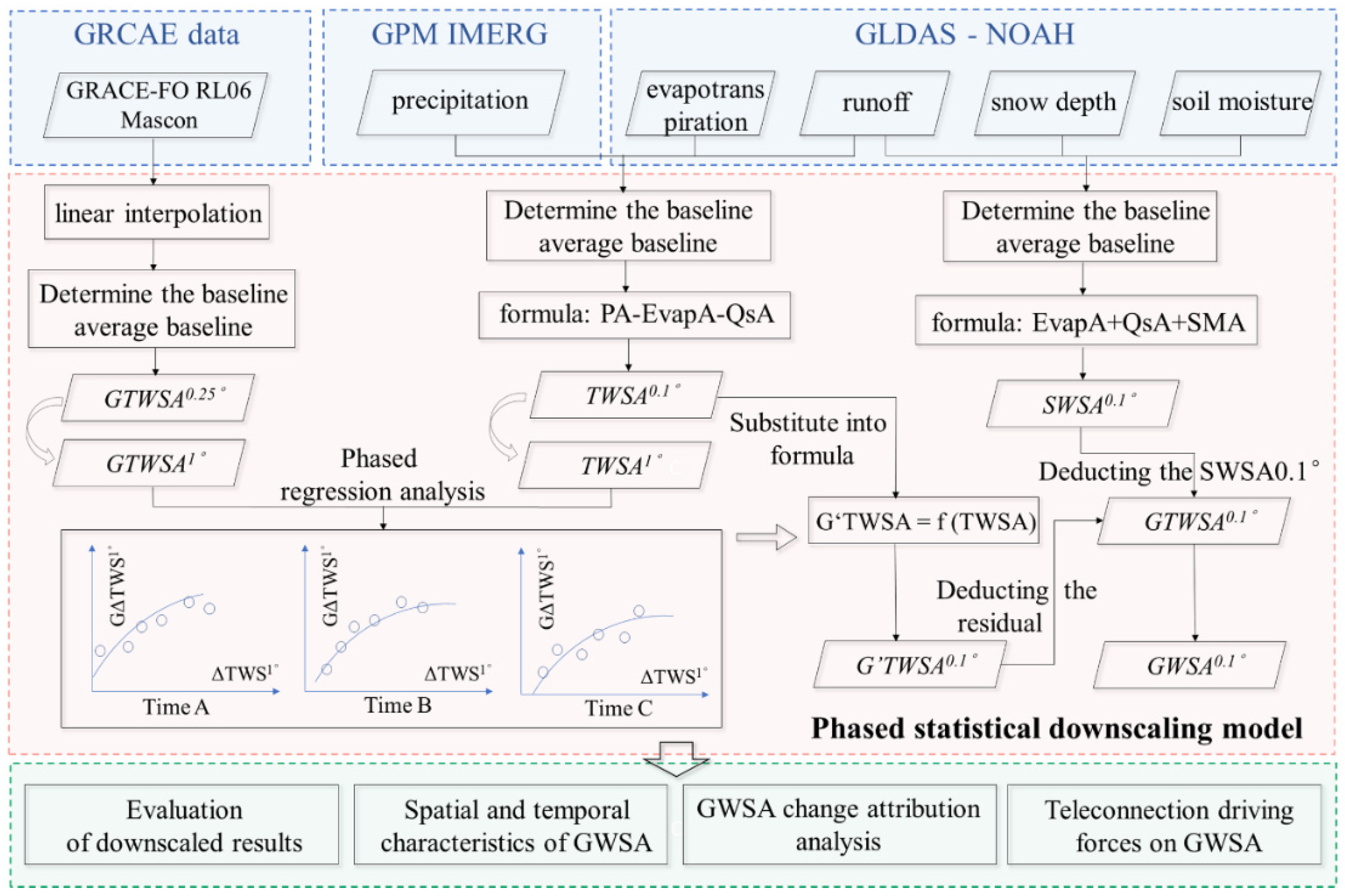
Firstly, the rainfall, runoff, and evapotranspiration data with a resolution of 1° are used to calculate the TWSA (water balance method). Secondly, the regression function is constructed between the TWSA (water balance method) and the GRACE-based TWSA (GTWSA). Thirdly, according to the regression function, the high-precision downscaled GRACE-based TWSA data is obtained. Finally, the downscaled ground water storage anomalies (GWSA) can be calculated. The flow chart representing the methodology is depicted in Figure 2.
3.1. Calculation of Groundwater Storage
The water balance method is the basis for the study of hydrological processes and the calculation of water storage [40]. Before the gravity satellite was launched and used, the water balance method was usually selected. The equation of water balance in the watershed system is expanded as follows:
where TWSA is calculated based on the water balance method; PA is precipitation anomalies; QsA is runoff anomalies; EvapA is evapotranspiration anomalies. The GLDAS model provides monthly evapotranspiration and runoff data, and IMERG provides monthly precipitation data. In order to facilitate the calculation, the dimension is converted into a unified unit (mm).
Because canopy water storage is small in the research area, the surface water in the study area is composed of snow depth, runoff, and soil moisture [41]. Therefore, the GWSA is calculated by the Formula (2):
where SWEA is the snow depth anomalies, QsA is the surface runoff anomalies, and SMA is the soil moisture anomalies of 0–200 cm. The three data are all obtained from the GLDAS model, and GTWSA is obtained from the GRACE data.
3.2. Phased Statistical Downscaling Model
GTWSA is the terrestrial water storage anomalies obtained from the GRACE data, which is calculated according to GRACE-FO RL06 mascon solutions. Although the CSR GRACE mascon data are represented by a grid of 0.25°, they represent an equal area geodesic grid with a size of 1 × 1° at the equator, so the CSR-GRACE mascon data are resampled to data with a resolution of 1°. When the TWSA1° of the Tibetan Plateau is moved backward one month relative to the GTWSA1°, the correlation coefficient increases from 0.33 to 0.46 using cross-correlation, so there is a one-month lag relationship between the TWSA1° and the GTWSA1°. Additionally, the Root Mean Squared Error (RMSE) is calculated between the GRACE-based TWSA and downscaled TWSA, in order to better understand the model’s ability. The statistical downscaling steps are as follows:
Step 1: according to Formula (1), using rainfall, runoff, and evapotranspiration data with a resolution of 1°, TWSA1° is calculated;
Step 2: the resolution of the CSR GRACE mascon data is resampled to 1° to obtain the GTWSA1°;
Step 3: the regression function relationship between the TWSA1° and the GTWSA1° is constructed by Formula (3):
Where G′TWSA is the TWSA fitted by the linear regression model.
The difference between the G’TWSA1° and the GTWSA1° is calculated as the residual of the downscaling system;
Step 4: according to the Formula (1), using the monthly Evap, P and Qs data with a resolution of 0.1°, the TWSA0.1° is calculated, and the G’TWSA0.1° is obtained according to the Formula (3);
Step 5: deducting the system residual from step 3 in the G’TWSA0.1°, then the downscaled TWSA with a resolution of 0.1° is obtained;
Step 6: calculate the downscaled GWSA according to the Formula (2).
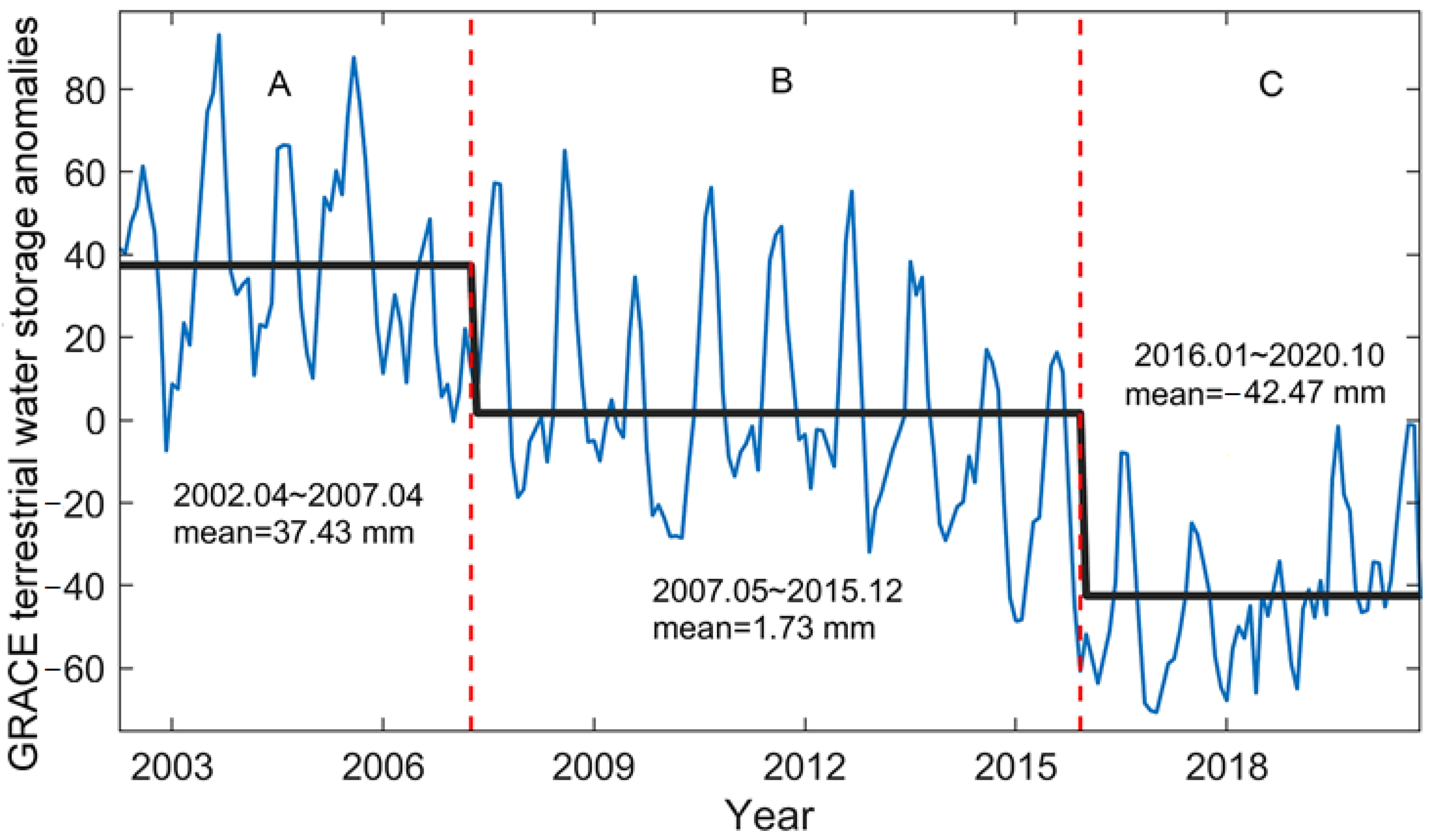
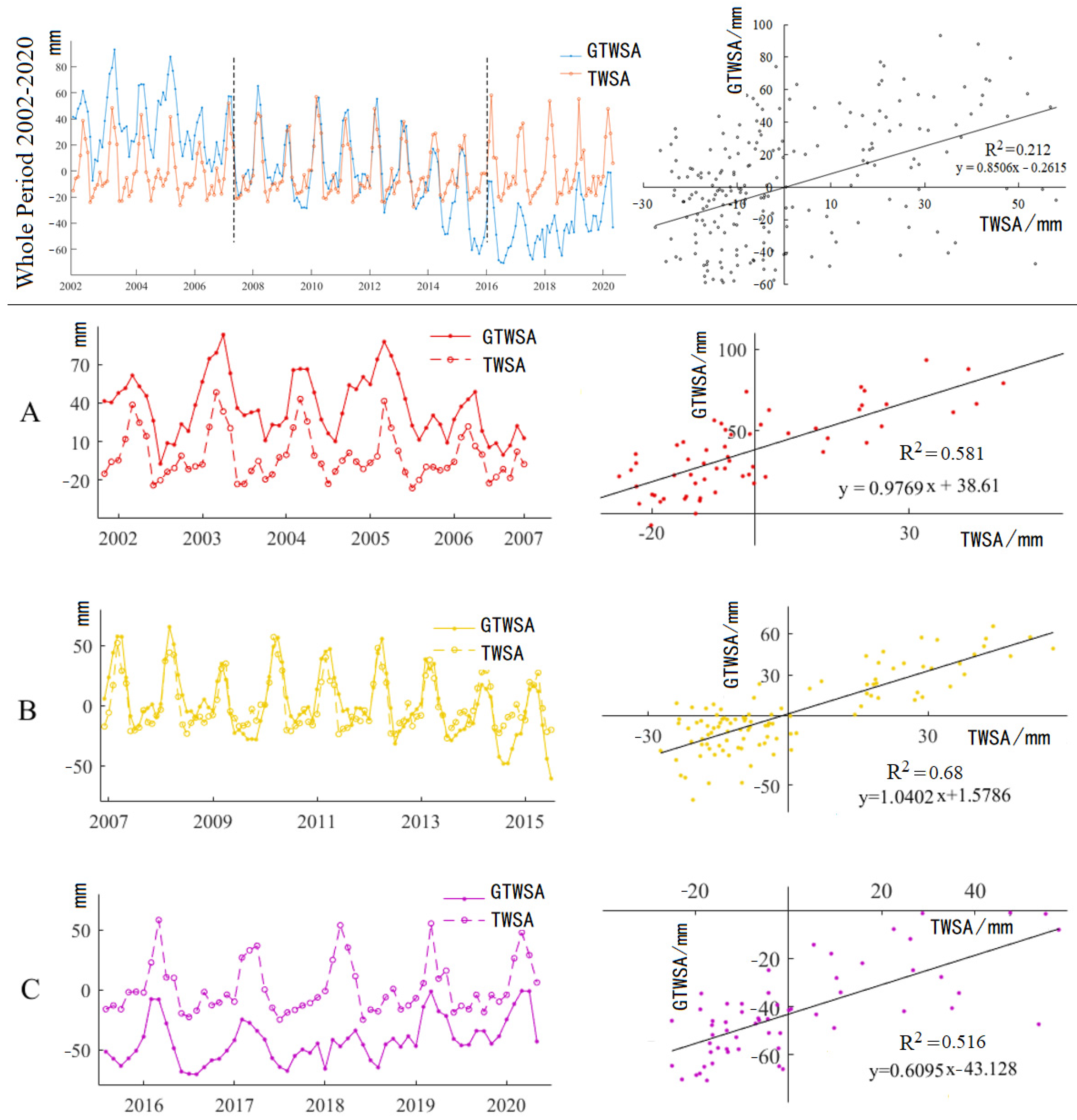
Since GTWSA and TWSA time series in different periods are fluctuating, it is difficult to get a good regression function relationship in step 3. We divided the whole period (2002 to 2020) into several stages based on the Bernaola Galvan segmentation algorithm. The Bernaola Galvan segmentation algorithm is a suitable method for phase division of nonsmooth, nonlinear time series. Compared with traditional methods, the Bernaola Galvan segmentation algorithm can segment non-stationary sequences into multiple stationary subsequences with different means [42,43]. The GRACE TWSA time series were divided into three segments, A (2002.4–2007.4), B (2007.5–2015.12) and C (2016.1–2020.10), as shown in Figure 3. After the phase division of the GRACE TWSA time series, the statistical regression relationship between the GTWSA (GRACE) and the TWSA (water balance method) is established by using a phased linear regression model. As shown in Figure 4, the original relationship between GTWSA and TWSA is low (R2 = 0.212) for the whole period (2002–2020). After the segmentation, the relationship was enhanced obviously in three stages, A (2002.4–2007.4 with R2 = 0.581), B (2007.5–2015.12 with R2 = 0.68) and C (2016.1–2020.10 with R2 = 0.516). A phased statistical downscale model is proposed to improve the effectiveness for obtaining downscaled GWSA.
3.3. Spatiotemporal Analysis Method
3.3.1. Extreme-Point Symmetric Mode Decomposition
In this study, the ESMD method is used to decompose the time series of the GWSA to study the variation period and trend of the GWSA in the Tibetan Plateau. The extreme-point symmetric mode decomposition (ESMD) method is an improvement of the traditional Hilbert–Huang transform based on the Fourier transform. ESMD has strong adaptability and local characteristics and is suitable for nonlinear and non-stationary time series analysis [44]. The ESMD method decomposes the original time series into a series of intrinsic mode function (IMF) components and a trend (R). The period of each IMF component can be obtained by a fast Fourier transform, and the trend term R represents the overall trend of the whole time series [45].
3.3.2. The Modified Mann–Kendall Trend Test
The MMK method is applied to reveal the change trend characteristics of the GWSA based on grid scale. The modified Mann–Kendall (MMK) trend test method can eliminate the autocorrelation component in the series and significantly improve the testability of the Mann–Kendall method, which is a nonparametric test method to effectively detect the changing trend of time series and is widely used in the field of hydro-meteorology [46,47].
3.4. Groundwater Storage Changes Attribution Analysis
The multiple linear regression model is usually used to study the relationship between changes in a dependent variable dependent on multiple independent variables and is one of the most widely used regression models, as shown in Equation (4) [48]. After standardizing all variables, the quantitative interpretation of the contribution of each variable can be given based on the standardized coefficients, as shown in Equation (5) [49].
where is the dependent variable, is the independent variable, is the intercept, is the standardized coefficient, and is the contribution rate of the independent variable.
The evapotranspiration and runoff data of the GLDAS NOAH2.1 model and the precipitation data of the GPM_IMERG V6 precipitation product are selected as natural factor data, and the prolonged artificial nighttime-light dataset of China is selected as the human activity data [50]. Since the natural factor of glacier melting is not considered, the contribution of human activities may be overestimated. The contribution rate of natural factors and human activities to climate change is calculated by the standardized coefficients of the multiple linear regression model, and then the attribution of climate change is quantitatively analyzed.
3.5. Cross Wavelet Transform
The cross wavelet transform can reveal the common power and relative phase in time-frequency space between two sequences, and the region with large transform coefficient represents that the two signals have strong correlation. In this study, the cross wavelet transform method is adopted to clarify the influence of teleconnection factors on the change of the GWSA on the Tibetan plateau.
4. Results
4.1. Evaluation of Downscaled Results
4.1.1. Comparison of GRACE-Based and Downscaled GTWSA
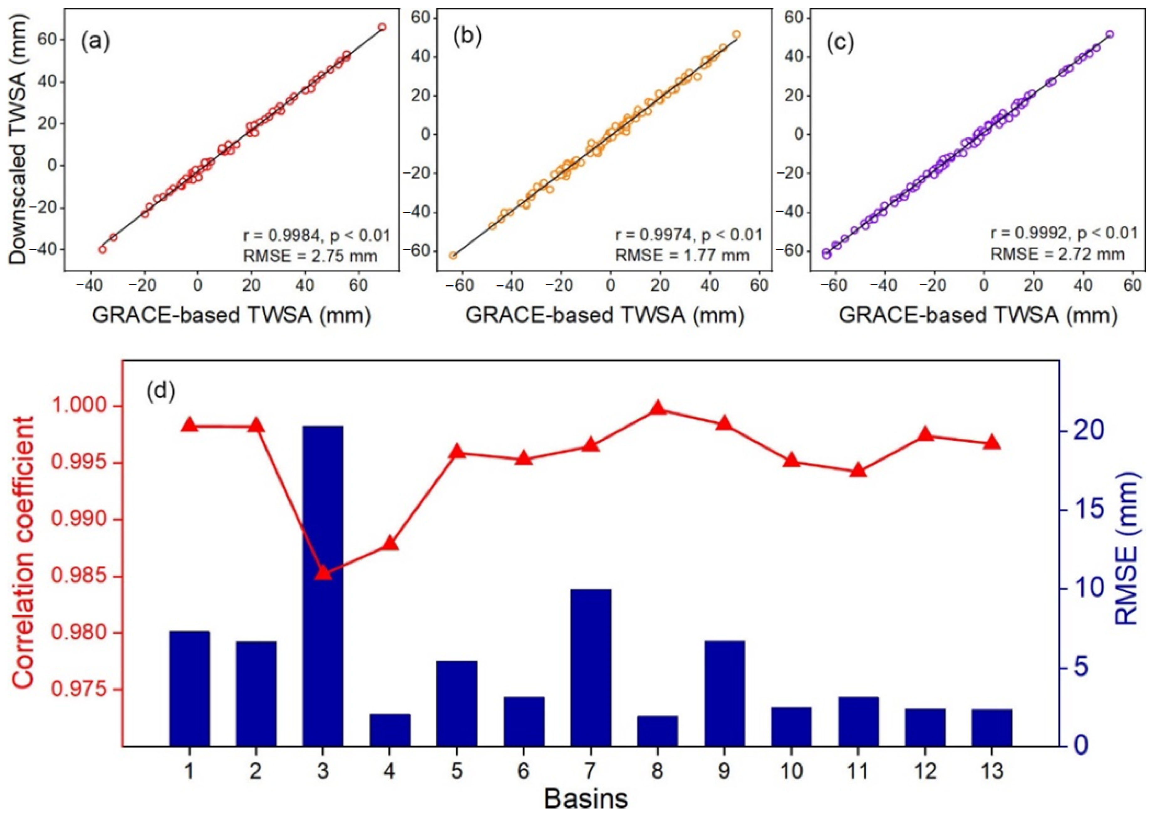
The temporal comparison of the TWSA and downscaled TWSA data in three stages A (2002.4–2007.4), B (2007.5–2015.12), and C (2016.1–2020.10) were tested using cell averaging, and the reliability of the downscaled results in the 12 sub-basins and the Tibetan Plateau were examined. By calculating monthly cell average value (2002.4–2020.10), time series comparison between GRACE-based TWSA and downscaled GTWSA were analyzed and shown in Figure 5. We use monthly cell average value (2002.4–2020.10) representing the whole region or sub-basin. Overall, the correlations between the downscaled data and GRACE data in three time series are high (r > 0.997) and the root mean square error (RSME < 2.75 mm) is low. Among them, the downscaled data in section B has the lowest RMSE (1.77 mm), and the downscaled data in section C has the highest correlation coefficient (r = 0.9992). Therefore, the time series data before and after downscaling are highly consistent. Spatially, the Tibetan Plateau can be subdivided into 12 sub-basins, and the correlation coefficients of the data before and after the downscaling of each sub-basin fluctuate between 0.9878–0.9997, and the overall correlation coefficient can reach 0.9967, and all of them are significantly correlated. The RSME of the 12 sub-basins is relatively small, and the maximum RSME of the Ganges River Basin is 24.34 mm. The smallest RSME in the Qaidam Basin is 1.91 mm, and the RSME in the Tibetan Plateau as a whole is 2.34 mm. The downscaling data almost completely maintain the time series variation characteristics of GRACE data, and the conservation of mass in sub-basins also existed objectively.
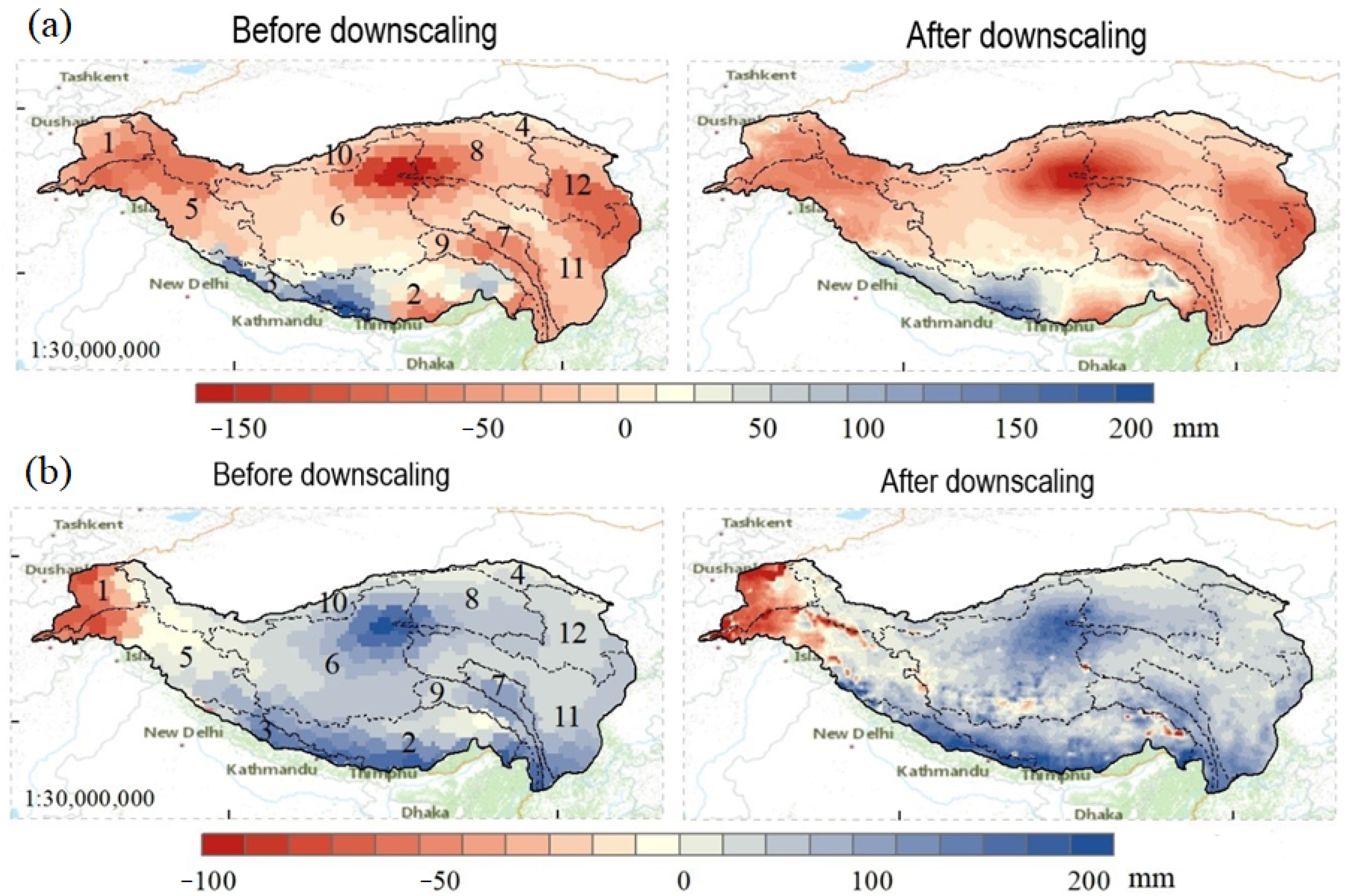
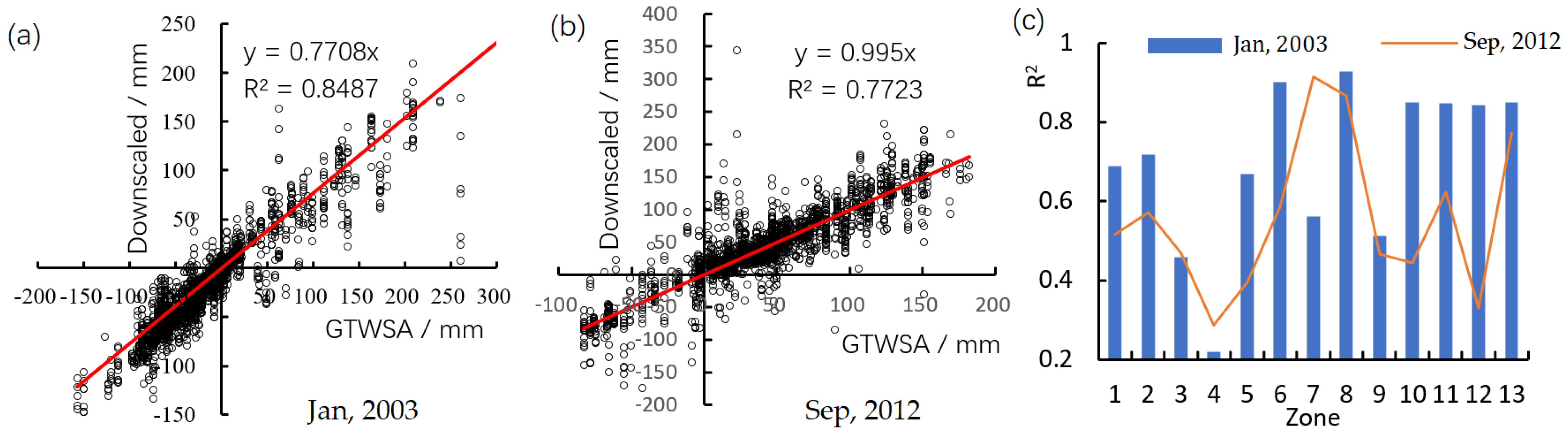
The spatial comparison of the GTWSA and downscaled GTWSA data in January 2003 and September 2012 were tested in the 12 sub-basins and the Tibetan Plateau. As shown in Figure 6, the downscaled data had finer spatial variation characteristics than the original GRACE data, especially in regions with larger absolute values. In Figure 7, by using 200 random sampling points, corresponding cell value were used to verify the reliability of the downscaled results in the 12 sub-basins and the Tibetan Plateau. Overall, the correlations are high (R2 > 0.77) between the downscaled GTWSA and GTWSA in these two periods. Spatially, the correlation coefficients in 12 sub-basins are various. Most of them are higher than 0.7, and the correlation coefficients in Qaidam are 0.866 and 0.929 in two periods. However, the correlation coefficients in both periods are very low in the Hexi Corridor.
4.1.2. Accuracy of Downscalsed GWSA
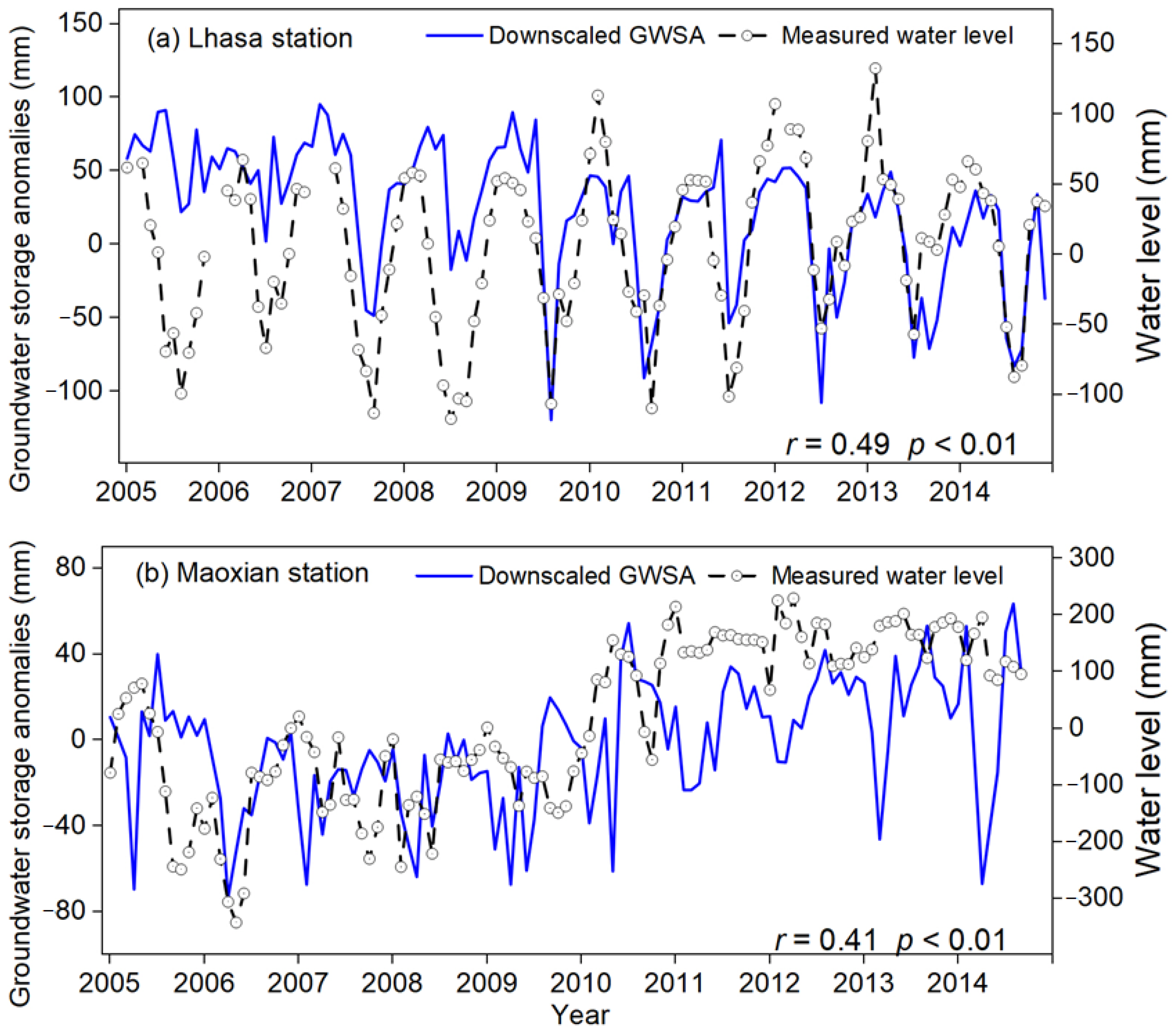
Due to there are very sparse observation wells in the vast Qinghai Tibet Plateau. Two observation wells (Lhasa Station and Maoxian Station from 2005 to 2014) with relatively complete data were used to verify the measured groundwater level and the downscaled GWSA, as shown in Figure 8. The downscaling results of GWSA effectively capture the interannual variation of groundwater, and the two curves have similar trend characteristics. The groundwater level observations of the Lhasa and Maoxian stations have a good correlation with the downscaled GWSA of the corresponding locations, the correlation coefficients are 0.49 and 0.41 respectively, and both pass the significance level test of 1%.
4.2. Spatial and Temporal Characteristics of GWSA
4.2.1. Spatial and Temporal Variations of GWSA
The interannual spatial variation of GWSA in the Tibetan Plateau from 2002 to 2020 is shown in Figure 9. The GWSA deficit area in the central Tibetan Plateau decreased year by year from 2002 to 2010. After 2010, the GWSA in the Inner Basin, the Qaidam Basin, the eastern Tarim Basin, and the upper reaches of the Yangtze Basin in the central region gradually turned positive. The GWSA spatial distribution pattern of the Tibetan Plateau has reversed from 2002 to 2020, which may be affected by recent global climate change.
The interannual fluctuations of the GWSA are shown in Figure 10. The GWSA on the Tibetan Plateau shows a downward trend (−0.45 mm/yr) from 2002 to 2020, as shown in Figure 10a. The annual changes of the GWSA in 12 sub-basins are shown in Figure 10b. The annual average GWSA variations in the Brahmaputra basin and the Ganges basin are decreasing and have become negative by the end of the study time in both locations. The Inner basin and the Qaidam Basin, on the other hand, change in the opposite trend, with a more pronounced upward trend in the last years of continuous groundwater accumulation. The annual average GWSA of sub-basins fluctuated smoothly in the range of ±50 mm from 2008 to 2014, while the annual average GWSA of each sub-watershed in 2002–2008 and 2014–2020 fluctuated more. In general, the fluctuations of sub-basins in the mid-term were small and concentrated, while the fluctuations at the beginning and end of the study were more intense.
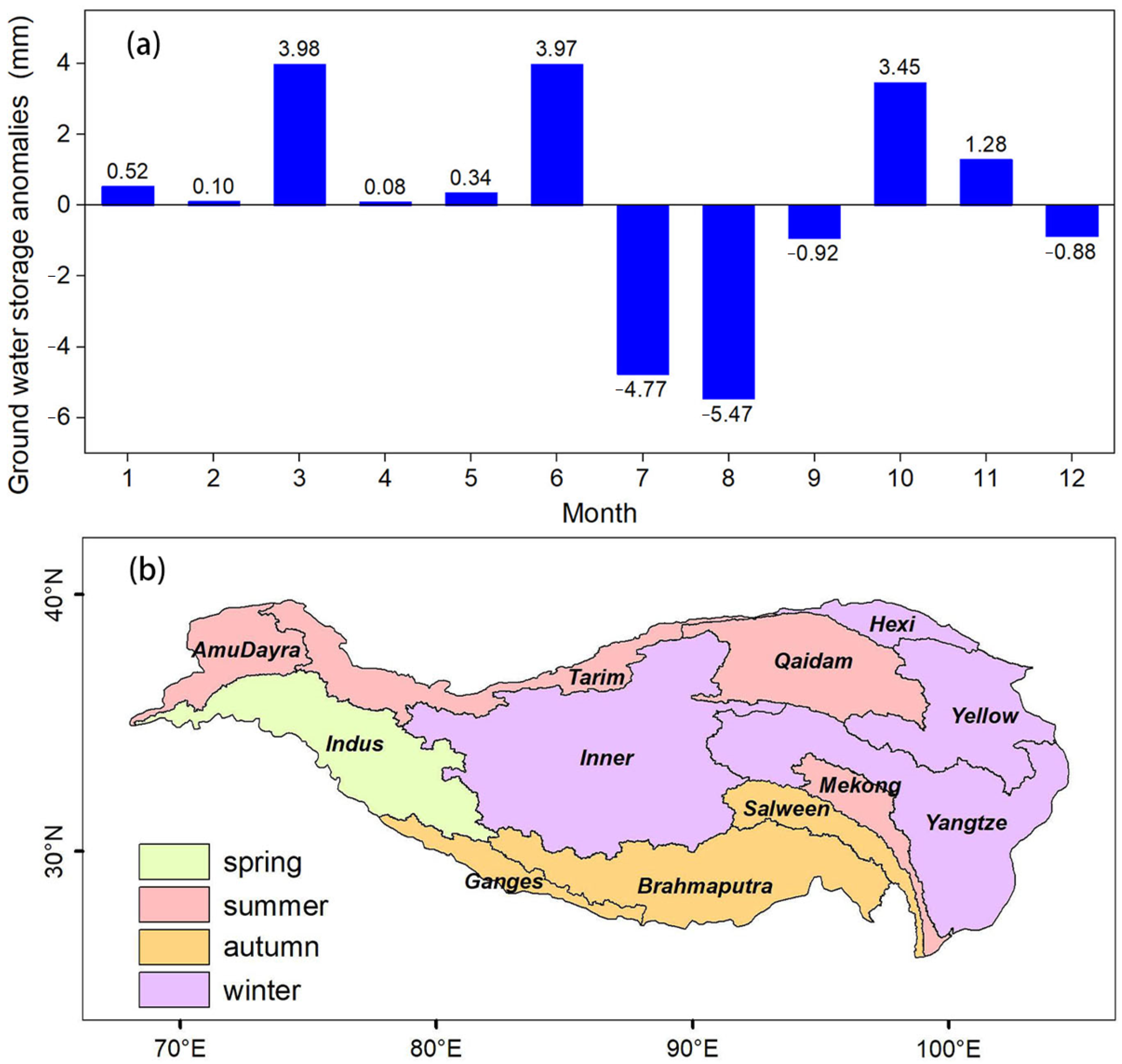
Figure 11a shows the monthly average GWSA on the Tibetan Plateau during the study period. The water balance on the Tibetan Plateau shows a large intra-annual oscillation, with the GWSA reaching its lowest value in July and August and its highest value in March and June. According to geological knowledge, the plateau climate is dominated by monsoon winds, and tropical tropospheric easterly winds, subtropical westerly winds and stratospheric easterly winds can bring a lot of precipitation to the plateau, but in summer, precipitation only accumulates on the surface of the plateau, and it takes some time for groundwater to produce flow. After October, the plateau climate enters a dry and cold period, when the rivers dry up and freeze, and groundwater replenishment is impeded, while in the spring, groundwater rises significantly when the temperature rises and large amounts of snow and ice melt. The frequency analysis of seasonal maxima is carried out for each sub-basin to better understand the spatial characteristics of GWSA in different seasons. Spring on the Qinghai–Tibet Plateau is March, April and May, and the specific months of summer, autumn and winter are obtained in turn. The number of months containing the maximum value in each season is counted, and the season with the highest number represents the seasonal color of the whole basin, as shown in Figure 11b. The dominant regions in winter occupy the central and eastern parts of the Tibetan Plateau; in autumn, all regions are concentrated in the Ganges, Brahmaputra, and Salween basins; in summer, all regions are distributed in the three basins in the northern part of the plateau except for the Mekong basin; in spring, there is only one Indus basin.
4.2.2. Periodic Characteristics of GWSA
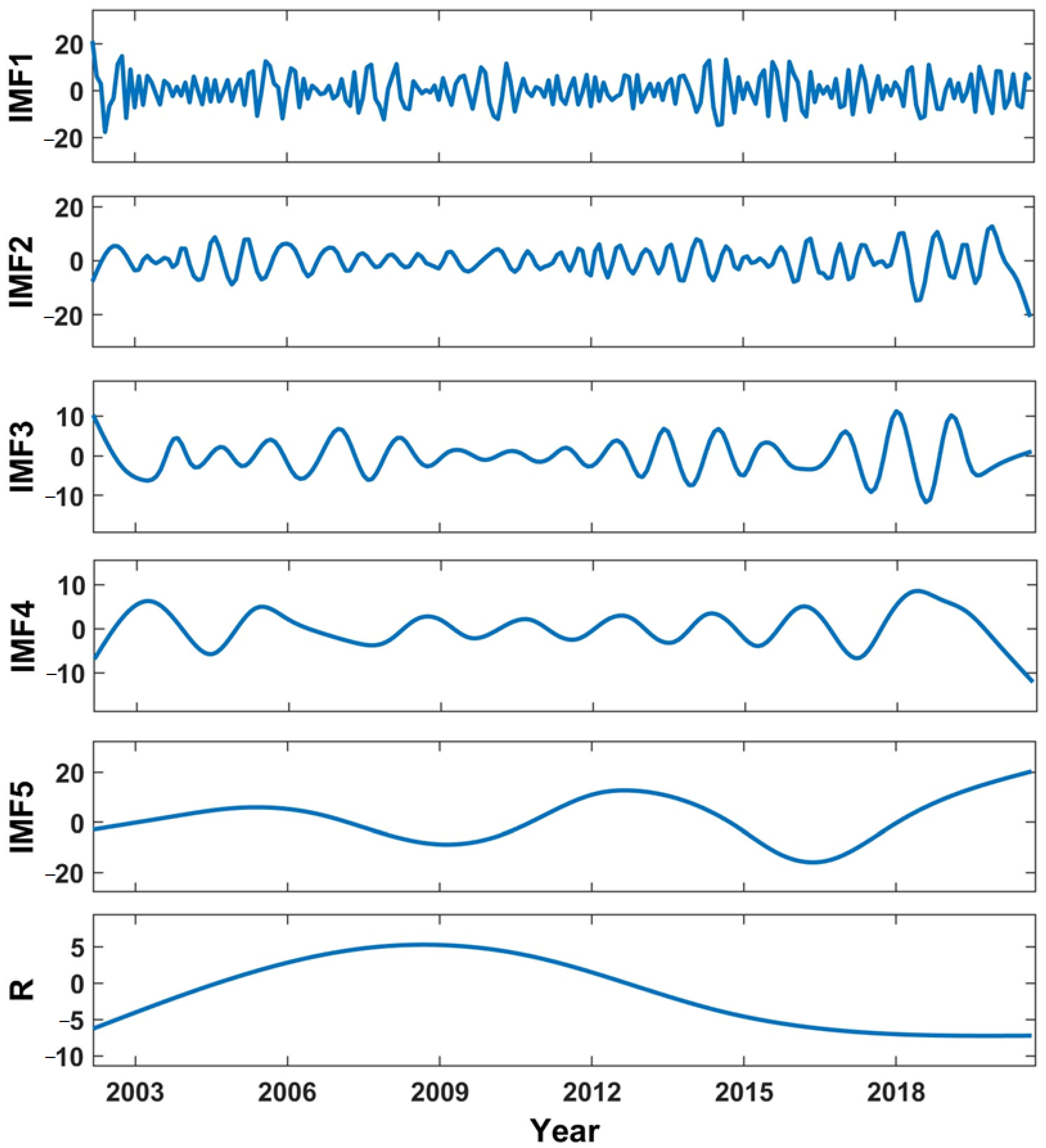
As shown in Figure 12, the original GWSA time series is decomposed into five IMF components (IMF1-IMF5) and one trend term (R). The sum of these IMF components and trend term completely coincides with the original GWSA sequence, which indicates that the ESMD method is complete and the decomposition result is reliable. The GWSA on the Tibetan Plateau shows a trend of increasing, then decreasing, and finally stabilizing from 2002 to 2020. To analyze the multi-time scale oscillation inherent in the time series of the GWSA, the average periods of each component are calculated by a fast Fourier transform, as shown in Table 2. The main periods of IMF1-IMF5 are 0.43, 0.55, 1.03, 2.65, and 4.65 years, respectively. This shows that the GWSA in the Tibetan Plateau has periodic characteristics of 0.43 years and 0.55 years on the annual scale, and periodic characteristics of 1.03 years, 2.65 years, and 4.65 years on the interannual scale. Meanwhile, the importance of each IMF component to the original series can be obtained from the variance contribution rate in Table 2. The variance contribution rate of 4.65 years for IMF5 is the largest, with a value of 37.58% and a very obvious oscillation signal, followed by the variance contribution rate of 0.43 years period for IMF1, with a value of 23.14%. Therefore, the variability of the GWSA time series in the Tibetan Plateau is mainly determined by IMF5 and IMF1, with the first and second principal periods of 4.65 and 0.43 years, respectively.
4.2.3. Trend Characteristics of GWSA
The GWSA trend characteristics of the Tibetan Plateau from 2002 to 2020 based on the MMK gridded trend test method are shown in Figure 13. The GWSA trend of the Tibetan Plateau exhibits significant spatial heterogeneity at the 0.05 level, which also reflects the unique topographic and climatic conditions of different regions of the Tibetan Plateau. Specifically, the GWSA in the western part of the Tibetan Plateau and the eastern part except the Yangtze basin indicates a decreasing trend, with the Brahmaputra basin showing the most obvious decreasing trend, reaching −13.84 mm/yr. However, the GWSA in the Inner, Tarim, and Yangtze basins show an upward trend, in which the rising trend of Inner is the most obvious, reaching 4.40 mm/yr, which may be affected by glacier melting caused by climate change in recent years [51]. Specifically, the GWSA of the Lhasa station shows a downward trend, while the GWSA of the Maoxian station shows an upward trend, which is consistent with the results obtained in Section 4.1.2.
4.3. GWSA Change Attribution Analysis
The contribution of natural factors and human activities to the GWSA changes on the Tibetan Plateau and its sub-basins are quantified based on the multiple linear regression, as shown in Table 3. The goodness-of-fit of the multiple linear regression models on the sub-basins of the Tibetan Plateau ranged from 0.21 to 0.89, with most of the basins having a goodness-of-fit of more than 0.6, indicating the reliability of the multiple linear regression model results. The GWSA changes of the Tibetan Plateau are dominated by natural factors, which is consistent with the sparsely populated nature of the Tibetan Plateau. However, there are some individual basins where human activities dominate. Due to the climate warming caused by human activities in recent years, there exists a non-negligible accelerated glacier melting on the Tibetan Plateau, which in turn has an impact on the spatial and temporal changes of groundwater. However, due to the difficulty in obtaining accurate glacier melt data, the natural factor of glacier melt was not considered in this study, which may have overestimated the impact of human activities.
4.4. Teleconnection Driving Forces on GWSA
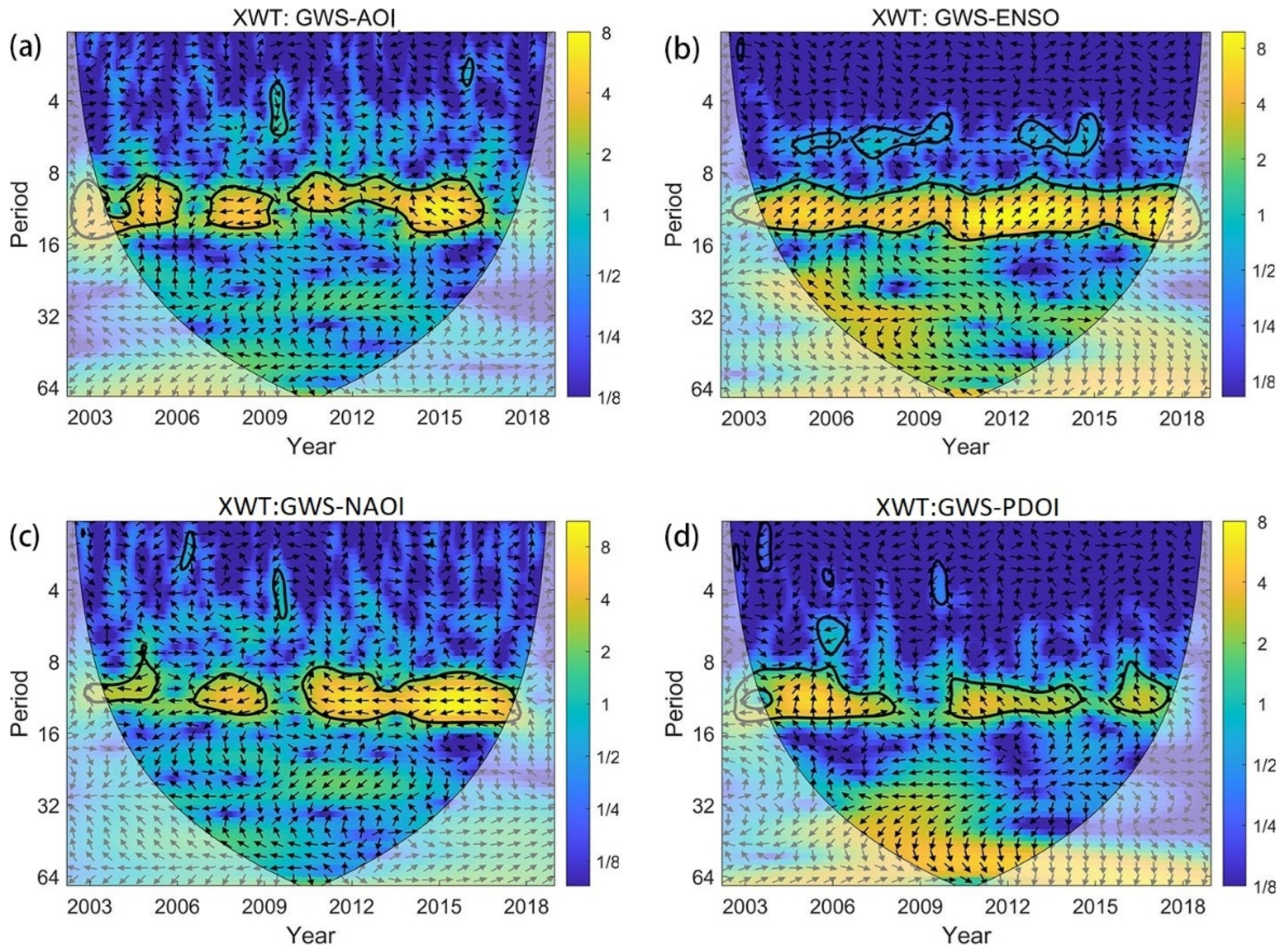
Groundwater changes are not only affected by natural factors and human activities, but also highly influenced by the teleconnection factors. The influence of teleconnection factors (AOI, ENSO, NAOI, PDOI) on the change of the GWSA on the Tibetan plateau is revealed by cross wavelet transform, as shown in Figure 14. There are three significant resonance periods between the GWSA and AOI, which are 8–16 months for 2003–2006 with negative correlation, 10–14 months for 2007–2008 with negative correlation, and 32–40 months for 2010–2016 with negative correlation, as shown in Figure 14a. Figure 14b shows that there is a long-term significant resonance period between the GWSA and ENSO that almost covers the study period and is largely positively correlated. Figure 14c demonstrates that there are three significant resonance periods between the GWSA and NAOI, 8–10 months from 2003–2005, 10–12 months from 2006–2009, and 8–16 months from 2010–2018, and all three resonance periods are positively correlated. There are three significant resonance periods between the GWSA and PDOI, 8–14 months for 2003–2006 with a positive correlation, 10–14 months for 2010–2014 with a negative correlation, and 8–12 months for 2015–2018 with a negative correlation (Figure 14d). The cross wavelet transform can effectively reveal the dynamic relationship between the GWSA and teleconnection factors on the Tibetan Plateau. The teleconnection factors have a significant statistical correlation with the GWSA on the Tibetan Plateau, indicating that they play an important role in the change of the GWSA on the Tibetan Plateau. It can be seen from the cross wavelet transform that the area of significant correlation between ENSO and GWSA is the largest among the teleconnection factors. In general, ENSO has the greatest influence on the GWSA on the Tibetan Plateau, while AOI, NAOI, and PDOI have similar and smaller effects on the GWSA on the Tibetan Plateau.
5. Discussion
Currently, groundwater storage estimation based on GRACE data has been widely used in many areas [52,53,54]. Recognizing how GWS responds to climate change is essential for future water availability and water resources management in the Tibetan Plateau. Compared with other areas, glaciers contribute to the most GWS variations in the Tibetan Plateau. However, the dominant factor controlling long-term GWS variation and its responses to climate change are not well understood. Famous for the Asian Water Tower, the Tibetan Plateau plays a critical role in providing water resources for more than two billion people living downstream [55]. A better understanding of GWS changes is essential for water resources management to ensure water security and food production [56].
Furthermore, GRACE data can be used to assess regional groundwater storages in deserts and remote mountainous areas [57,58]. Related research shows that GRACE data can make up for the shortcomings of groundwater monitoring networks and show great potential in tracking changes in groundwater storages [59]. However, GRACE data have the problem of low spatial resolution. Normally the spatial resolution of GRACE data is about 350 km, which is higher than most groundwater research areas scale [60]. Chambers [61] performed first-order polynomial fitting of all even (odd) orders of the same order to improve the resolution of GRACE data when calculating changes in seawater mass. Gao et al. [62] combined the distribution of regional hydrogeological parameters to refine the GRACE data (downscaling). Our results showed that the trend of GWSA in the Tibetan Plateau exhibited significant spatial heterogeneity, which was consistent with the findings of Xiang et al. [63]. The GWSA in the Inner, Tarim, and Yangtze basins showed an increasing trend, which was comparable to Zhang et al. [64]. The western part of the Tibetan Plateau and the eastern region, except the Yangtze basin, showed a decreasing trend in GWSA, which seemed to be different from Zou et al. [65]. Zou et al. concluded that the GWS increased during 2003–2016 in all subdivisions of the Tibetan Plateau, except for the Inner Plateau. However, GRACE-based GWS change estimates still contain large uncertainties [66]. In contrast, this paper used the linear regression method to downscale the terrestrial water storage, constructing a GWSA dataset based on a phased statistical downscaling model. The downscaled GWSA is reliable in both time and space, and is consistent with the groundwater level trend of ground observation wells. Therefore, the phased statistical downscaling model proposed in this paper is reliable in the Tibetan Plateau. Furthermore, this study provides a comprehensive and detailed analysis of the spatial and temporal characteristics, periodic patterns, spatiotemporal trends, and driving factors of groundwater storage changes on the Tibetan Plateau, which provides a reference for groundwater resource management on the Tibetan Plateau. It is useful and convenient to use this method to study other areas by considering temporal variation over a long period.
GWSA change attribution analysis results indicate that the GWSA changes of the Tibetan Plateau are dominated by natural factors (Table 3). Noticeably, the average contributions of natural factors and human factors are 62% and 38%, respectively. Among the natural factors, compared with precipitation and runoff, evaporation is the main factor affecting the change of GWSA, with an average value of 27%. In total, the attributions of 10 basins are more than 20%. Furthermore, the human factors are mainly reflected by the contribution of night lights, which ranges from 20% (in the AmuDayra and Hexi basins) to 61% (in the Qaidam basin). The contribution of human activities to the change of groundwater storage in the Qaidam basin is 61%, which may be related to the construction of hydraulic facilities for agricultural development in the Qaidam basin in recent years and the extensive ecological restoration works in the area [67]. As for the AmuDayra and Hexi watersheds, where the contribution of natural factors is high, the former is an extensive uninhabited area and the latter is adjacent to the Qilian Mountains National Nature Reserve, where development has been restricted in recent years.
Among teleconnection factors, ENSO, a strong signal of global climate change, is a climatic phenomenon that occurs when the ocean and atmosphere interact and lose their balance, often arousing the atmospheric circulation change, leading to global climate anomalies [68]. Lu et al. [69] found that North China had the strongest response to ENSO by analyzing the correlation between the affected area ratio and the disaster area ratio of drought in various regions of China from 1949 to 1990. Zhang et al. [70] showed that ENSO events have a greater impact on the drought and flood changes in the Qinling Mountains. In general, ENSO has the greatest influence on the GWSA on the Tibetan Plateau. Zhu et al. [71] have also shown that ENSO has a certain impact on the change of groundwater storage in the southeast of the Tibetan Plateau, and the impact of ENSO is relatively strong in areas with significant loss of water storage.
However, there are still shortcomings in the current study. First, there are several institutions providing GRACE data products, and this paper only selects one of them for calculation. However, some studies have shown that the arithmetic averaging of GRACE data products from different institutions gives more accurate data on the TWSA [72,73]. Filling in the missing GRACE data with linear interpolation may also bring about uncertainties [74]. Secondly, the statistical downscaling method relies on the correlation between model data and GRACE data, and the method needs to be carried out in the edge-regularized area and then clipped according to the basin boundary, which may introduce more edge leakage errors. Thirdly, limited by the availability of data, the number of observation wells used for verifying the accuracy of the downscaled GWSA is a little small. Only the time series data of the two observation stations are relatively complete, which is one of the limitations of this paper. Finally, the GWSA is obtained by subtracting precipitation, evapotranspiration, and snow from the GRACE TWSA, but does not take into account the influence of lakes and reservoirs, so the accuracy of downscaled GWSA can be further improved. In the future, groundwater level fluctuations can also be simulated and predicted with a desirable accuracy using artificial neural network and intelligence models [75,76].
6. Conclusions
To improve the low spatial resolution of gravity satellite data products, this study successfully downscaled the GWSA on the Tibetan Plateau based on a phased statistical downscaling model and tested the reliability of the downscaling results at the spatial and temporal scales. Second, the spatiotemporal variation of groundwater storage from 2002 to 2020 is analyzed by using the downscaled GWSA data. Finally, a quantitative attribution analysis of the drivers of the GWSA changes on the Tibetan Plateau is conducted based on a multiple linear regression model. Then, the cross wavelet transform is used to analyze the relationship between groundwater and teleconnection factors. The main conclusions are as follows:
- (1)
- The correlation coefficients of the data before and after downscaling exceed 0.99 in the all-time series, and the RSME is low, while the data before and after downscaling in the 12 sub-basins also show high correlation. The groundwater levels measured at the Lhasa and Maoxian stations and the GWSA after downscaling of the corresponding grid show consistent trends, and are significantly correlated at the 0.01 level.
- (2)
- From the perspective of long time series, the GWSA in the Tibetan Plateau shows a downward trend (−0.45 mm/yr) from 2002 to 2020, but experiences a trend of increasing, then decreasing, and finally stabilizing. The variation trend of the GWSA in the Tibetan Plateau shows significant spatial heterogeneity, and the GWSA in the Inner, Tarim, and Yangtze basins indicate a significant upward trend, while those in the western part of the Tibetan Plateau and the eastern region, except the Yangtze basin, show a significant downward trend, in which the Brahmaputra basin has the most obvious downward trend, reaching −13.84 mm/yr.
- (3)
- The GWSA changes in the Tibetan Plateau are mainly dominated by natural factors, which is in line with the characteristics of “vast land and sparsely populated” in the Tibetan Plateau. However, the impact of human activities can not be ignored in individual sub-basins. The results of cross wavelet transform show that ENSO has the greatest influence on the GWSA on the Tibetan Plateau.
The downscaling of GRACE and the study of the temporal and spatial variation of groundwater in the Tibetan Plateau still have certain challenges. Accurate GWSA data are helpful to land use, urban planning, and water resources management. This study provides high-resolution GWSA data products on the Tibetan Plateau, which can effectively provide regional groundwater storage change dynamics and provide data support for managers to formulate policies, such as balancing the relationship between regional irrigation water use and groundwater consumption, and can help evaluate regional groundwater consumption more effectively.
Author Contributions
Conceptualization, Z.L. and G.G.; methodology, G.G. and J.W.; validation, G.G. and J.Z.; investigation, G.G. and J.W.; writing—original draft preparation, G.G.; writing—review and editing, J.Z., J.C. and G.Z.; supervision, Z.L.; project administration, Z.L.; funding acquisition, Z.L. All authors have read and agreed to the published version of the manuscript.
Funding
This research was funded by Distribution and transformation of pharmaceutical and personal care products in groundwater in the middle and lower reaches of the Yellow River region of the National Natural Science Foundation of China, grant number 41972261.
Acknowledgments
CSR GRACE mascon data are provided by the National Aeronautics and Space Administration (NASA) Making Earth System Data Records for Use in Research Environments (MEaSUREs) Program and are available at http://www2.csr.utexas.edu/grace/RL06_mascons.html, accessed on 1 March 2021. GLDAS data are provided by the National Aeronautics and Space Administration Land Data Assimilation System (http://ldas.gsfc.nasa.gov/gldas/, accessed on 1 March 2021). We also thank the Chinese Ecosystem Research Network (CERN) for providing the groundwater observation data and the Integrated Multi-satellite Retrievals for GPM (IMERG) (https://disc.gsfc.nasa.gov/datasets/GPM_3IMERGM_06/summary, accessed on 1 March 2021) for providing the precipitation data.
Conflicts of Interest
The authors declare no conflict of interest.
References
- Zhao, M.; Geruo, A.; Zhang, J.; Velicogna, I.; Liang, C.; Li, Z. Ecological restoration impact on total terrestrial water storage. Nat. Sustain. 2020, 4, 56–62. [Google Scholar] [CrossRef]
- de Graaf, I.E.M.; Gleeson, T.; van Beek, L.P.H.R.; Sutanudjaja, E.H.; Bierkens, M.F.P. Environmental flow limits to global groundwater pumping. Nature 2019, 574, 90–94. [Google Scholar] [CrossRef]
- Rodell, M.; Famiglietti, J.S.; Wiese, D.N.; Reager, J.T.; Beaudoing, H.K.; Landerer, F.W.; Lo, M.H. Emerging trends in global freshwater availability. Nature 2018, 557, 651–659. [Google Scholar] [CrossRef]
- Bibi, S.; Wang, L.; Li, X.; Zhang, X.; Chen, D. Response of Groundwater Storage and Recharge in the Qaidam Basin (Tibetan Plateau) to Climate Variations From 2002 to 2016. J. Geophys. Res. Atmos. 2019, 124, 9918–9934. [Google Scholar] [CrossRef]
- Huang, Z.; Pan, Y.; Gong, H.; Yeh, P.J.-F.; Li, X.; Zhou, D.; Zhao, W. Subregional-scale groundwater depletion detected by GRACE for both shallow and deep aquifers in North China Plain. Geophys. Res. Lett. 2015, 42, 1791–1799. [Google Scholar] [CrossRef]
- Feng, W.; Shum, C.; Zhong, M.; Pan, Y. Groundwater Storage Changes in China from Satellite Gravity: An Overview. Remote Sens. 2018, 10, 674. [Google Scholar] [CrossRef] [Green Version]
- Wang, F.; Wang, Z.; Yang, H.; Di, D.; Zhao, Y.; Liang, Q. Utilizing GRACE-based groundwater drought index for drought characterization and teleconnection factors analysis in the North China Plain. J. Hydrol. 2020, 585, 124849. [Google Scholar] [CrossRef]
- Wu, T.; Zheng, W.; Yin, W.; Zhang, H. Spatiotemporal Characteristics of Drought and Driving Factors Based on the GRACE-Derived Total Storage Deficit Index: A Case Study in Southwest China. Remote Sens. 2020, 13, 79. [Google Scholar] [CrossRef]
- Miro, M.; Famiglietti, J. Downscaling GRACE Remote Sensing Datasets to High-Resolution Groundwater Storage Change Maps of California’s Central Valley. Remote Sens. 2018, 10, 143. [Google Scholar] [CrossRef] [Green Version]
- Yin, W.; Hu, L.; Zhang, M.; Wang, J.; Han, S.-C. Statistical Downscaling of GRACE-Derived Groundwater Storage Using ET Data in the North China Plain. J. Geophys. Res. Atmos. 2018, 123, 5973–5987. [Google Scholar] [CrossRef]
- Vishwakarma, B.D.; Zhang, J.; Sneeuw, N. Downscaling GRACE total water storage change using partial least squares regression. Sci. Data 2021, 8, 95. [Google Scholar] [CrossRef] [PubMed]
- Zhang, J.; Liu, K.; Wang, M. Downscaling Groundwater Storage Data in China to a 1-km Resolution Using Machine Learning Methods. Remote Sens. 2021, 13, 523. [Google Scholar] [CrossRef]
- Qi, L.Q.; Su, X.L.; Feng, K. Response of multi-scale meteorological drought to circulation index in north west China. J. Arid Land Resour. Environ. 2020, 34, 106–114. [Google Scholar] [CrossRef]
- Crausbay, S.D.; Betancourt, J.; Bradford, J.; Cartwright, J.; Dennison, W.C.; Dunham, J.; Enquist, C.A.; Frazier, A.G.; Hall, K.R.; Litte, J.S.; et al. Unfamiliar Territory: Emerging Themes for Ecological Drought Research and Management. One Earth 2020, 3, 337–353. [Google Scholar] [CrossRef]
- Ouyan, R.; Liu, W.; Fu, G.B.; Liu, C.M.; Hu, L.; Wang, H. Linkages between ENSO/PDO signals and precipitation, streamflow in China during the last 100 years. Hydrol. Earth Syst. Sci. 2014, 11, 4235–4265. [Google Scholar] [CrossRef] [Green Version]
- Thompson, D.W.J.; Wallace, J.M. The Arctic Oscillation signature in the wintertime geopotential height and temperature fields. Geophys. Res. Lett. 1998, 25, 1297–1300. [Google Scholar] [CrossRef] [Green Version]
- Liu, Y.; Ni, Y.Q. Diagnostic research of the effects of ENSO on the Asian summer monsoon circulation and the summer precipitation in China. Acta Meteorol. Sin. 1998, 56, 681–691. [Google Scholar]
- Feng, J.; Chen, W. Interference of the East Asian winter monsoon in the impact of ENSO on the East Asian summer monsoon in decaying phases. Adv. Atmos. Sci. 2014, 31, 344–354. [Google Scholar] [CrossRef]
- Luterbacher, J.; Schmutz, C.; Gyalistras, D.; Xoplaki, E.; Wanner, H. Reconstruction of monthly NAO and EU indices back to AD 1675. Geophys. Res. Lett. 1999, 26, 2745–2748. [Google Scholar] [CrossRef] [Green Version]
- Ma, Z.G.; Shao, L.J. Relationship between dry/wet variation and the Pacific decade oscillation (PDO) in Northern China during the last 100 years. Chin. J. Atmos. Sci. 2006, 30, 464–474. [Google Scholar] [CrossRef]
- Zhan, P.; Song, C.; Luo, S.; Ke, L.; Liu, K.; Chen, T. Investigating different timescales of terrestrial water storage changes in the northeastern Tibetan Plateau. J. Hydrol. 2022, 608, 127608. [Google Scholar] [CrossRef]
- Wang, L.; Wang, J.; Wang, L.; Zhu, L.; Li, X. Terrestrial water storage regime and its change in the endorheic Tibetan Plateau. Sci. Total Environ. 2022, 815, 152729. [Google Scholar] [CrossRef] [PubMed]
- Li, X.; Long, D.; Scanlon, B.R.; Mann, M.E.; Li, X.; Tian, F.; Sun, Z.; Wang, G. Climate change threatens terrestrial water storage over the Tibetan Plateau. Nat. Clim. Chang. 2022, 12, 801–807. [Google Scholar] [CrossRef]
- Xu, Z.; Cheng, L.; Luo, P.; Liu, P.; Zhang, L.; Li, F.; Liu, L.; Wang, J. A Climatic Perspective on the Impacts of Global Warming on Water Cycle of Cold Mountainous Catchments in the Tibetan Plateau: A Case Study in Yarlung Zangbo River Basin. Water 2020, 12, 2338. [Google Scholar] [CrossRef]
- Sun, S.; Bao, C.; Tang, Z. Tele-connecting water consumption in Tibet: Patterns and socio-economic driving factors for virtual water trades. J. Clean. Prod. 2019, 233, 1250–1258. [Google Scholar] [CrossRef]
- Deng, H.; Pepin, N.C.; Liu, Q.; Chen, Y. Understanding the spatial differences in terrestrial water storage variations in the Tibetan Plateau from 2002 to 2016. Clim. Chang. 2018, 151, 379–393. [Google Scholar] [CrossRef] [Green Version]
- Deng, H.; Chen, Y.; Chen, X. Driving factors and changes in components of terrestrial water storage in the endorheic Tibetan Plateau. J. Hydrol. 2022, 612, 128225. [Google Scholar] [CrossRef]
- Zhang, G. Dataset of River Basins Map over the TP (2016); National Tibetan Plateau Data Center: Beijing, China, 2019. [Google Scholar] [CrossRef]
- Zhang, G.; Yao, T.; Xie, H.; Kang, S.; Lei, Y. Increased mass over the Tibetan Plateau: From lakes or glaciers? Geophys. Res. Lett. 2013, 40, 2125–2130. [Google Scholar] [CrossRef]
- Tapley, B.D.; Watkins, M.M.; Flechtner, F.; Reigber, C.; Bettadpur, S.; Rodell, M.; Sasgen, I.; Famiglietti, J.S.; Landerer, F.W.; Chambers, D.P.; et al. Contributions of GRACE to understanding climate change. Nat. Clim. Chang. 2019, 5, 358–369. [Google Scholar] [CrossRef] [PubMed]
- Save, H.; Bettadpur, S.; Tapley, B.D. High-resolution CSR GRACE RL05 mascons. J. Geophys. Res. Solid Earth 2016, 121, 7547–7569. [Google Scholar] [CrossRef]
- Scanlon, B.R.; Zhang, Z.; Save, H.; Wiese, D.N.; Landerer, F.W.; Long, D.; Longuevergne, L.; Chen, J. Global evaluation of new GRACE mascon products for hydrologic applications. Water Resour. Res. 2016, 52, 9412–9429. [Google Scholar] [CrossRef] [Green Version]
- Fatolazadeh, F.; Eshagh, M.; Goita, K. A new approach for generating optimal GLDAS hydrological products and uncertainties. Sci. Total Environ. 2020, 730, 138932. [Google Scholar] [CrossRef]
- Li, X.; Long, D.; Han, Z.; Scanlon, B.R.; Sun, Z.; Han, P.; Hou, A. Evapotranspiration Estimation for Tibetan Plateau Headwaters Using Conjoint Terrestrial and Atmospheric Water Balances and Multisource Remote Sensing. Water Resour. Res. 2019, 55, 8608–8630. [Google Scholar] [CrossRef]
- Wang, F.; Lai, H.X.; Li, Y.B.; Feng, K.; Zhang, Z.Z.; Tian, Q.Q.; Zhu, X.M.; Yang, H.B. Identifying the status of groundwater drought from a GRACE mascon model perspective across China during 2003–2018. Agric. Water Manag. 2022, 260, 107251. [Google Scholar] [CrossRef]
- Pradhan, R.K.; Markonis, Y.; Godoy, M.R.V.; Villalba-Pradas, A.; Andreadis, K.M.; Nikolopoulos, E.I.; Papalexiou, S.M.; Rahim, A.; Tapiador, F.J.; Hanel, M. Review of GPM IMERG performance: A global perspective. Remote Sens. Environ. 2022, 268, 112754. [Google Scholar] [CrossRef]
- Tang, G.; Clark, M.P.; Papalexiou, S.M.; Ma, Z.; Hong, Y. Have satellite precipitation products improved over last two decades? A comprehensive comparison of GPM IMERG with nine satellite and reanalysis datasets. Remote Sens. Environ. 2020, 240, 111697. [Google Scholar] [CrossRef]
- Huffman, G.J.; Stocker, E.F.; Bolvin, D.T.; Nelkin, E.J.; Jackson, T. GPM IMERG Final Precipitation L3 1 Month 0.1 Degree x 0.1 Degree V06; Goddard Earth Sciences Data and Information Services Center (GES DISC): Greenbelt, MD, USA, 2016. [Google Scholar] [CrossRef]
- Höhle, J.; Höhle, M. Accuracy assessment of digital elevation models by means of robust statistical methods. Isprs J. Photogramm. 2009, 64, 398–406. [Google Scholar] [CrossRef] [Green Version]
- Xie, J.; Xu, Y.P.; Gao, C.; Xuan, W.; Bai, Z. Total Basin Discharge From GRACE and Water Balance Method for the Yarlung Tsangpo River Basin, Southwestern China. J. Geophys. Res. Atmos. 2019, 124, 7617–7632. [Google Scholar] [CrossRef]
- Thomas, B.F.; Famiglietti, J.S. Identifying Climate-Induced Groundwater Depletion in GRACE Observations. Sci. Rep. 2019, 9, 4124. [Google Scholar] [CrossRef]
- Bernaola-Galvan, P.; Ivanov, P.C.; Amaral, L.A.N.; Stanley, H.E. Scale invariance in the nonstationarity of human heart rate. Phys. Rev. Lett. 2001, 87, 168105. [Google Scholar] [CrossRef] [Green Version]
- Wang, F.; Wang, Z.; Yang, H.; Zhao, Y. Study of the temporal and spatial patterns of drought in the Yellow River basin based on SPEI. Sci. China Earth Sci. 2018, 61, 1098–1111. [Google Scholar] [CrossRef]
- Wang, J.-L.; Li, Z.-J. Extreme-Point Symmetric Mode Decomposition Method for Data Analysis. Adv. Adapt. Data Anal. 2013, 5, 1350015. [Google Scholar] [CrossRef]
- Li, H.-F.; Wang, J.-L.; Li, Z.-J. Application of ESMD Method to Air-Sea Flux Investigation. Int. J. Geosci. 2013, 04, 8–11. [Google Scholar] [CrossRef] [Green Version]
- Mallick, J.; Talukdar, S.; Alsubih, M.; Salam, R.; Ahmed, M.; Kahla, N.B.; Shamimuzzaman, M. Analysing the trend of rainfall in Asir region of Saudi Arabia using the family of Mann-Kendall tests, innovative trend analysis, and detrended fluctuation analysis. Theor. Appl. Climatol. 2020, 143, 823–841. [Google Scholar] [CrossRef]
- Yue, S.; Wang, C.Y. The Mann-Kendall test modified by effective sample size to detect trend in serially correlated hydrological series. Water Resour. Manag. 2004, 18, 201–218. [Google Scholar] [CrossRef]
- Kim, S.W.; Jung, D.; Choung, Y.-J. Development of a Multiple Linear Regression Model for Meteorological Drought Index Estimation Based on Landsat Satellite Imagery. Water 2020, 12, 3393. [Google Scholar] [CrossRef]
- Ding, Y.; Zang, R. Determinants of aboveground biomass in forests across three climatic zones in China. For. Ecol. Manag. 2021, 482, 118805. [Google Scholar] [CrossRef]
- Lixian, Z.; Zhehao, R.; Bin, C.; Peng, G.; Haohuan, F.; Bing, X. A Prolonged Artificial Nighttime-Light Dataset of China (1984–2020); National Tibetan Plateau Data Center: Beijing, China, 2021. [Google Scholar] [CrossRef]
- Wang, J.; Chen, X.; Hu, Q.; Liu, J. Responses of terrestrial water storage to climate variation in the Tibetan Plateau. J. Hydrol. 2020, 584, 124652. [Google Scholar] [CrossRef]
- Yeh, P.J.; Swenson, S.; Famiglietti, J.S.; Rodell, M. Remote sensing of groundwater storage changes in Illinois using the Gravity Recovery and Climate Experiment (GRACE). Water Resour. Res. 2006, 42, W12203. [Google Scholar] [CrossRef]
- Moore, S.; Fisher, J.S. Challenges and Opportunities in GRACE-Based Groundwater Storage Assessment and Management: An Example from Yemen. Water Resour. Manag. 2012, 26, 1425–1453. [Google Scholar] [CrossRef]
- Cao, Y.P.; Nan, Z.T. Applications of GRACE in hydrology: A review. Remote Sens. Technol. Appl. 2011, 26, 543–553. [Google Scholar] [CrossRef]
- Immerzeel, W.W.; van Beek, L.P.H.; Bierkens, M.F.P. Climate change will affect the Asian Water Towers. Science 2010, 328, 1382–1385. [Google Scholar] [CrossRef]
- Immerzeel, W.W.; Bierkens, M.F.P. Asia’s water balance. Nat. Geosci. 2012, 5, 841–842. [Google Scholar] [CrossRef]
- Rodell, M.; Chen, J.; Kato, H.; Famiglietti, J.S.; Nigro, J.; Wilson, C.R. Estimating groundwater storage changes in the Mississippi River basin (USA) using GRACE. Hydrogeol. J. 2007, 15, 159–166. [Google Scholar] [CrossRef] [Green Version]
- Yin, W.J.; Hu, L.T.; Wang, J.R. Changes of groundwater storage variation based on GRACE data at the Beishan area, Gansu Province. Hydrogeol. Eng. Geol. 2015, 42, 29–34. [Google Scholar] [CrossRef]
- Swenson, S.; Yeh, J.F.; Wahr, J.; Famiglietti, J. A comparison of terrestrial water storage variations from GRACE with in situ measurements from Illinois. Geophys. Res. Lett. 2006, 33, 627–642. [Google Scholar] [CrossRef] [Green Version]
- Hu, L.T.; Sun, K.N.; Yin, W.J. Review on the application of GRACE satellite in regional groundwater management. J. Earth Sci. Environ. 2016, 38, 258–266. [Google Scholar] [CrossRef]
- Chambers, D.P. Evaluation of new grace time-variable gravity data over the ocean. Geophys. Res. Lett. 2006, 33, L17603. [Google Scholar] [CrossRef]
- Gao, Z.; Wei, G.; Chang, N.B. Integrating temperature vegetation dryness index (TVDI) and regional water stress index (RWSI) for drought assessment with the aid of LANDSAT TM/ETM+ images. Int. J. Appl. Earth Obs. Geoinf. 2011, 13, 495–503. [Google Scholar] [CrossRef]
- Xiang, L.W.; Wang, H.S.; Steffen, H.; Wu, P.; Jia, L.L.; Jiang, L.M.; Shen, Q. Groundwater storage changes in the Tibetan Plateau and adjacent areas revealed from GRACE satellite gravity data. Earth Planet. Sci. Lett. 2016, 449, 228–239. [Google Scholar] [CrossRef] [Green Version]
- Zhang, G.Q.; Yao, T.D.; Shun, C.K.; Yi, S.; Yang, K.; Xie, H.J.; Feng, W.; Bolch, T.; Wang, L.; Behrangi, A.; et al. Lake volume and groundwater storage variations in Tibetan Plateau’s endorheic basin. Geophys. Res. Lett. 2017, 44, 5550–5560. [Google Scholar] [CrossRef]
- Zou, Y.G.; Kuang, X.X.; Feng, Y.Q.; Jiao, J.J.; Liu, J.G.; Wang, C.; Fan, L.F.; Wang, Q.J.; Chen, J.X.; Ji, F.; et al. Solid Water Melt Dominates the Increase of Total Groundwater Storage in the Tibetan Plateau. Geophys. Res. Lett. 2022, 49, e2022GL100092. [Google Scholar] [CrossRef]
- Wang, L.; Wang, J.; Li, M.; Wang, L.; Li, X.; Zhu, L. Response of terrestrial water storage and its change to climate change in the endorheic Tibetan Plateau. J. Hydrol. 2022, 612, 128231. [Google Scholar] [CrossRef]
- Jia, H.; Yan, C.; Xing, X. Evaluation of Eco-Environmental Quality in Qaidam Basin Based on the Ecological Index (MRSEI) and GEE. Remote Sens. 2021, 13, 4543. [Google Scholar] [CrossRef]
- Sun, J.Q.; Yuan, W.; Gao, Y.Z. Arabian Peninsula-North Pacific Oscillation and its relationship with Asian summer monsoon. Sci. China 2008, 38, 750–762. [Google Scholar]
- Lu, A.G.; Ge, J.P.; Pang, D.Q.; He, Y.Q.; Pang, H.X. Asynchronous response of droughts to ENSO in China. J. Glaciol. Geocryol. 2006, 28, 535–542. [Google Scholar]
- Zhang, S.H.; Qi, G.Z.; Su, K.; Zhou, L.Y.; Meng, Q.; Bai, H.Y. Changes of drought and flood in the Qinling Mountains in the last 60 years. Acta Ecol. Sin. 2022, 42, 4758–4769. [Google Scholar] [CrossRef]
- Zhu, Y.; Liu, S.G.; Yi, Y.; Li, W.Q.; Zhang, S.D. Spatiotemporal Changes of Terrestrial Water Storage in Three Parallel River Basins and Its Response to ENSO. Mt. Res. 2020, 38, 165–179. [Google Scholar] [CrossRef]
- Zhang, J.; Liu, K.; Wang, M. Seasonal and Interannual Variations in China’s Groundwater Based on GRACE Data and Multisource Hydrological Models. Remote Sens. 2020, 12, 845. [Google Scholar] [CrossRef] [Green Version]
- Liu, B.; Zou, X.; Yi, S.; Sneeuw, N.; Cai, J.; Li, J. Identifying and separating climate- and human-driven water storage anomalies using GRACE satellite data. Remote Sens. Environ. 2021, 263, 112559. [Google Scholar] [CrossRef]
- Long, D.; Yang, Y.T.; Wada, Y.; Hong, Y.; Liang, W.; Chen, Y.N.; Yong, B.; Hou, A.Z.; Wei, J.F.; Chen, L. Deriving scaling factors using a global hydrological model to restore GRACE total water storage changes for China’s Yangtze River Basin. Remote Sens. Environ. 2015, 168, 177–193. [Google Scholar] [CrossRef]
- Samani, S.; Vadiati, M.; Azizi, F.; Zamani, E.; Kisi, O. Groundwater Level Simulation Using Soft Computing Methods with Emphasis on Major Meteorological Components. Water Resour. Manag. 2022, 36, 3627–3647. [Google Scholar] [CrossRef]
- Vadiati, M.; Yami, Z.R.; Eskandari, E.; Nakhaei, M.; Kisi, O. Application of artificial intelligence models for prediction of groundwater level fluctuations: Case study (Tehran-Karaj alluvial aquifer). Environ. Monit. Assess. 2022, 194, 619. [Google Scholar] [CrossRef]
Figure 1.
Sub-basin division of the Tibetan Plateau.

Figure 2.
The flow chart representing the methodology in this study.

Figure 3.
Phasing of the GRACE terrestrial water storage anomalies on the Tibetan Plateau from 2002 to 2020. (A) (2002.4–2007.4), (B) (2007.5–2015.12) and (C) (2016.1–2020.10).
Figure 3.
Phasing of the GRACE terrestrial water storage anomalies on the Tibetan Plateau from 2002 to 2020. (A) (2002.4–2007.4), (B) (2007.5–2015.12) and (C) (2016.1–2020.10).

Figure 4.
Relationship between GRACE terrestrial water storage anomalies (GTWSA) and TWSA in the whole period (2002–2020) and three phases the on the Tibetan Plateau. (A) (2002.4–2007.4), (B) (2007.5–2015.12) and (C) (2016.1–2020.10).
Figure 4.
Relationship between GRACE terrestrial water storage anomalies (GTWSA) and TWSA in the whole period (2002–2020) and three phases the on the Tibetan Plateau. (A) (2002.4–2007.4), (B) (2007.5–2015.12) and (C) (2016.1–2020.10).

Figure 5.
Accuracy test of downscale TWSA in different periods and basins in the Tibetan Plateau basin. (a–c) the accuracy verification results of A, B and C time series before and after downscaling, respectively. (d) the accuracy verification results of sub-basins 1–12 (AmuDayra, Brahmaputra, Ganges, Hexi, Indus, Inner, Mekong, Qaidam, Salween, Tarim, Yangtze, and Yellow) and 13 (Tibetan Plateau) before and after downscaling.

Figure 6.
Comparison of terrestrial water storage anomalies (GRACE TWSA) in the Tibetan Plateau before and after downscaling. (a) January 2003, (b) September 2012.
Figure 6.
Comparison of terrestrial water storage anomalies (GRACE TWSA) in the Tibetan Plateau before and after downscaling. (a) January 2003, (b) September 2012.

Figure 7.
Spatial comparison of downscale GTWSA and original GTWSA for the whole Tibetan Plateau by using almost 2400 random sampling points in January 2003 (a) and September 2012 (b), respectively. (c) spatial comparison in sub-basins 1–12 (AmuDayra, Brahmaputra, Ganges, Hexi, Indus, Inner, Mekong, Qaidam, Salween, Tarim, Yangtze, and Yellow) and 13 (Tibetan Plateau) before and after downscaling.

Figure 8.
Comparison of downscaled groundwater storage anomalies (GWSA) with observation well measurement results. (a) Lhasa Station; (b) Maoxian Station.
Figure 8.
Comparison of downscaled groundwater storage anomalies (GWSA) with observation well measurement results. (a) Lhasa Station; (b) Maoxian Station.

Figure 9.
Interannual spatial variation of groundwater storage changes in the Tibetan Plateau.

Figure 10.
(a) Groundwater storage anomalies time series and its trends in the Tibetan Plateau from 2002 to 2020. (b) The annual variations of groundwater storage anomalies in sub-basins of the Tibetan Plateau.
Figure 10.
(a) Groundwater storage anomalies time series and its trends in the Tibetan Plateau from 2002 to 2020. (b) The annual variations of groundwater storage anomalies in sub-basins of the Tibetan Plateau.

Figure 11.
Trends in groundwater storage change on the Tibetan Plateau from 2002 to 2020. (a) The average monthly; (b) The season of the biggest change.
Figure 11.
Trends in groundwater storage change on the Tibetan Plateau from 2002 to 2020. (a) The average monthly; (b) The season of the biggest change.

Figure 12.
Intrinsic mode function (IMF) components and trend (R) of groundwater storage anomalies in the Tibetan Plateau.
Figure 12.
Intrinsic mode function (IMF) components and trend (R) of groundwater storage anomalies in the Tibetan Plateau.

Figure 13.
Trend of groundwater storage anomalies in the Tibetan Plateau.

Figure 14.
Cross wavelet transform between groundwater storage anomalies and (a) AOI, (b) ENSO, (c) NAOI, and (d) PDOI in the Tibetan Plateau.
Figure 14.
Cross wavelet transform between groundwater storage anomalies and (a) AOI, (b) ENSO, (c) NAOI, and (d) PDOI in the Tibetan Plateau.


Table 1.
Data sources of the four climate factors (accessed on 1 March 2021).
| Climate Factor | Long Name | Data Source |
|---|---|---|
| AOI | Arctic Oscillation Index | https://www.ncdc.noaa.gov/teleconnections/ao/ |
| ENSO | El Nino-Southern Oscillation Index | http://www.esrl.noaa.gov/psd/data/correlation/nina34.data |
| NAOI | North Atlantic Oscillation Index | https:/www.ncdc.noaa.gov/teleconnections/nao/ |
| PDOI | Pacific Decadal Oscillation Index | http://www.ncdc.noaa.gov/teleconnections/pdo/ |
Table 2.
Periods, variance contributions and correlation coefficients of each component of groundwater storage in the Tibetan Plateau.
Table 2.
Periods, variance contributions and correlation coefficients of each component of groundwater storage in the Tibetan Plateau.
| IMF1 | IMF2 | IMF3 | IMF4 | IMF5 | R | |
|---|---|---|---|---|---|---|
| Period | 0.43 | 0.55 | 1.03 | 2.65 | 4.65 | |
| Variance contribution | 23.14% | 12.59% | 8.58% | 7.42% | 37.58% | 10.70% |
| Correlation coefficient | 0.48 ** | 0.38 ** | 0.30 ** | 0.23 ** | 0.57 ** | 0.27 ** |
Note: In the table, “**” represents passing the 1% level of significance.
Table 3.
Attribution analysis of groundwater storage changes on the Tibetan Plateau.
| Basins | R2 | Evaporation | Precipitation | Runoff | Night Lights | Natural | Human |
|---|---|---|---|---|---|---|---|
| Tibetan Plateau | 0.08 | 32% | 5% | 24% | 39% | 61% | 39% |
| AmuDayra | 0.32 | 33% | 36% | 11% | 20% | 80% | 20% |
| Brahmaputra | 0.79 | 9% | 11% | 30% | 50% | 50% | 50% |
| Ganges | 0.71 | 29% | 6% | 27% | 39% | 61% | 39% |
| Hexi | 0.69 | 46% | 32% | 3% | 20% | 80% | 20% |
| Indus | 0.73 | 23% | 18% | 15% | 43% | 57% | 43% |
| Inner | 0.83 | 26% | 7% | 32% | 35% | 65% | 35% |
| Mekong | 0.53 | 42% | 2% | 25% | 30% | 70% | 30% |
| Qaidam | 0.89 | 8% | 7% | 24% | 61% | 39% | 61% |
| Salween | 0.67 | 31% | 16% | 20% | 33% | 67% | 33% |
| Tarim | 0.21 | 32% | 11% | 24% | 33% | 67% | 33% |
| Yangtze | 0.41 | 26% | 9% | 17% | 48% | 52% | 48% |
| Yellow | 0.44 | 17% | 38% | 2% | 43% | 57% | 43% |
Publisher’s Note: MDPI stays neutral with regard to jurisdictional claims in published maps and institutional affiliations. |
© 2022 by the authors. Licensee MDPI, Basel, Switzerland. This article is an open access article distributed under the terms and conditions of the Creative Commons Attribution (CC BY) license (https://creativecommons.org/licenses/by/4.0/).
Share and Cite
MDPI and ACS Style
Gao, G.; Zhao, J.; Wang, J.; Zhao, G.; Chen, J.; Li, Z. Spatiotemporal Variation and Driving Analysis of Groundwater in the Tibetan Plateau Based on GRACE Downscaling Data. Water 2022, 14, 3302. https://doi.org/10.3390/w14203302
AMA Style
Gao G, Zhao J, Wang J, Zhao G, Chen J, Li Z. Spatiotemporal Variation and Driving Analysis of Groundwater in the Tibetan Plateau Based on GRACE Downscaling Data. Water. 2022; 14(20):3302. https://doi.org/10.3390/w14203302
Chicago/Turabian StyleGao, Guangli, Jing Zhao, Jiaxue Wang, Guizhang Zhao, Jiayue Chen, and Zhiping Li. 2022. "Spatiotemporal Variation and Driving Analysis of Groundwater in the Tibetan Plateau Based on GRACE Downscaling Data" Water 14, no. 20: 3302. https://doi.org/10.3390/w14203302
Note that from the first issue of 2016, this journal uses article numbers instead of page numbers. See further details here.