
The Impact of Land Cover on Selected Water Quality Parameters in Polish Lowland Streams during the Non-Vegetative Period


1
Department of Hydrology, Faculty of Geography and Regional Studies, University of Warsaw, Krakowskie Przedmieście 30, 00-927 Warsaw, Poland
2
Faculty of Geography and Regional Studies, University of Warsaw, Krakowskie Przedmieście 30, 00-927 Warsaw, Poland
*
Author to whom correspondence should be addressed.
Water 2022, 14(20), 3295; https://doi.org/10.3390/w14203295
Submission received: 18 September 2022
/
Revised: 14 October 2022
/
Accepted: 16 October 2022
/
Published: 19 October 2022
(This article belongs to the Special Issue Water, Wastewater, Waste Management in Agriculture and Agri-Food Industry)
Abstract
:The search for the best landscape predictors explaining the spatial variability of stream water chemistry is one of the most important and recent research issues. Thus, in the current study, relationships between land cover indices and selected water quality parameters were evaluated regarding the example of 54 lowland temperate streams located in central Poland. From November 2021 to March 2022, water samples were collected in the monthly timescale, and the concentrations of NH4+, NO3−, and NO2−, as well as electrical conductivity, were correlated with the percentage of land cover types calculated for total catchment area, buffer zones, cut buffer zones, and radius. For such computing, Corine Land Cover 2018 and Sentinel 2 Global Land Cover datasets were used. In the case of both datasets, results indicate significant dependence of NO3−, and NO2− concentrations, as well as EC values on cover metrics. Overall, agricultural lands favored higher concentrations of NO3− and NO2−, whereas mainly coniferous forests reduced nitrogen pollution. Significant correlations were not documented in the case of NH4+ ions, the concentrations of which could be linked to point sources from municipal activity. Correlation performance was slightly better in the case of the S2GLC dataset, while the best spatial scales were generally seen for wider buffer zones (250 and 500 m) and total catchment area. The study provided spatially extensive insight into the impact of land cover predictors at different scales on nitrogen compounds in a lowland landscape.
1. Introduction
The deterioration of water quality is still a significant challenge both in developing and developed countries [1,2]. Human activities alter all water systems [3], but major attention has been paid to rivers, which are considered a chief source of renewable water supply for humans and freshwater ecosystems [3]. In the United States, one-third of rivers have been classified as polluted, in China—over 45% [4]. In Europe, approximately 60% of flowing waters have an unsatisfactory ecological status [5]. Furthermore, water quality and quantity issues are poised to be more aggravated due to environmental alterations, such as climate changes and the intensification of the hydrological cycle [6,7]. Both hydrochemistry and water quantity are significantly affected by land use and land cover (LULC) changes [8,9]. Landscape composition and configuration control hydrological processes [10] and nutrient sources, as well as their mobilization and migration across the catchments [4]. Agricultural activities which require extensive areas are especially charged with responsibility for N and P loads runoff, causing water contamination [11,12]. According to [13], 38% of water bodies in the European Union are under pressure from agricultural pollution. The eutrophication of freshwaters, driven mainly by agriculture [14], results not only in the lack of potable water for humans [15], but also jeopardizes biodiversity [3]. These problems may be intensified during certain seasons; for example, in the cold season, the critical aggravation of water quality can be related to the intensification of erosion processes due to small cover or a lack of vegetation, as well as the impeded infiltration of snowmelt and rainwater when the ground is frozen [16]. Simultaneously, such deterioration is caused by organic matter decomposition, including by macrophytes [17]. Rivers are peculiar water bodies, since the effects of overenrichment of flowing waters in nutrients are explicit in lake ecosystems [18], as well as marine ecosystems that experience anoxia and hypoxia, especially in coastal zones [19,20]. Such areas, called dead zones, occur across the globe, and one of them is located in the Baltic Sea [21].
To counteract the further destabilization of lotic ecosystems, appropriate management should be implemented. Management needs to be based on copious research on variable factors and take advantage of those that fit particular environmental conditions. So far, many studies covering LULC-water quality relationships have emerged [4,22]. Ref. [23] highlighted three stages of research on the effects of land use and land cover changes on water quality; the last stage is characterized by the use of remote sensing, GIS, and multivariate analysis. Recent reports in this research trend have covered almost all continents; thus, different environmental contexts have been taken into account. For instance, study areas differ in terms of hydroclimatological conditions–from arid [24,25] and semi-arid [26,27], through temperate [28,29], to tropical [30]. The most common technique used to analyze water quality problems was statistical modeling, since it is a simpler, more understandable, and more efficient method than physically based modeling [22]. Scientists adopted different methods to identify appropriate explanatory variables: non-spatial land use metrics, such as PLAND (percentage of the landscape belonging to a given class) [31,32], the inverse distance weighted method, where landscape metrics closer to the water body are more important [33,34], landscape configuration metrics [35,36], and the riparian zone approach [37,38]. Different land use and land cover data were also used from low-resolution datasets, from Corine Land Cover [39,40], to high-resolution maps derived from the classification of satellite images [41,42].
Despite the abundance of studies on water-quality-related topics, there are still some gaps to fill in with new study areas, materials, and approaches. One of the challenges set before contemporary water quality research using GIS is the availability and characteristics of land use/land cover datasets and their effectiveness in explaining variations in water quality. There is a need to evaluate the performance of widely available and cost-free datasets, with an aim for results to be comparable on a Europe-wide scale. Such comparisons are especially welcome in lowland catchments, which seem to be less frequently represented, as land–water interactions were mainly investigated in uplands [43]. First order streams (in Strahler’s system) are important components of nutrient spiraling. They play a major role in the recycling of nutrients, according to [44,45], or are as important as with higher order rivers, according to [46]. Due to the fact that small watercourses are rarely subject to government monitoring, it is necessary to conduct field research. Usually, such investigations are limited to a dozen or so sampling points [35,36,47,48].
Therefore, this paper provides a spatially extensive investigation of relationships between selected nutrient compounds and land cover across small lowland catchments during the cold, non-vegetative season. The specific objectives of the study were to (a) assess the spatial patterns of nitrates, nitrites, and ammonium concentrations in lowland streams; (b) evaluate the performance of land cover characteristics that affect these nitrogen compounds’ variability; (c) determine the best spatial scale of land cover metrics explaining the concentrations of nitrogen compounds; and (d) evaluate the performance of landscape metrics computed with two different, but widely available and cost-free datasets.
2. Study Area
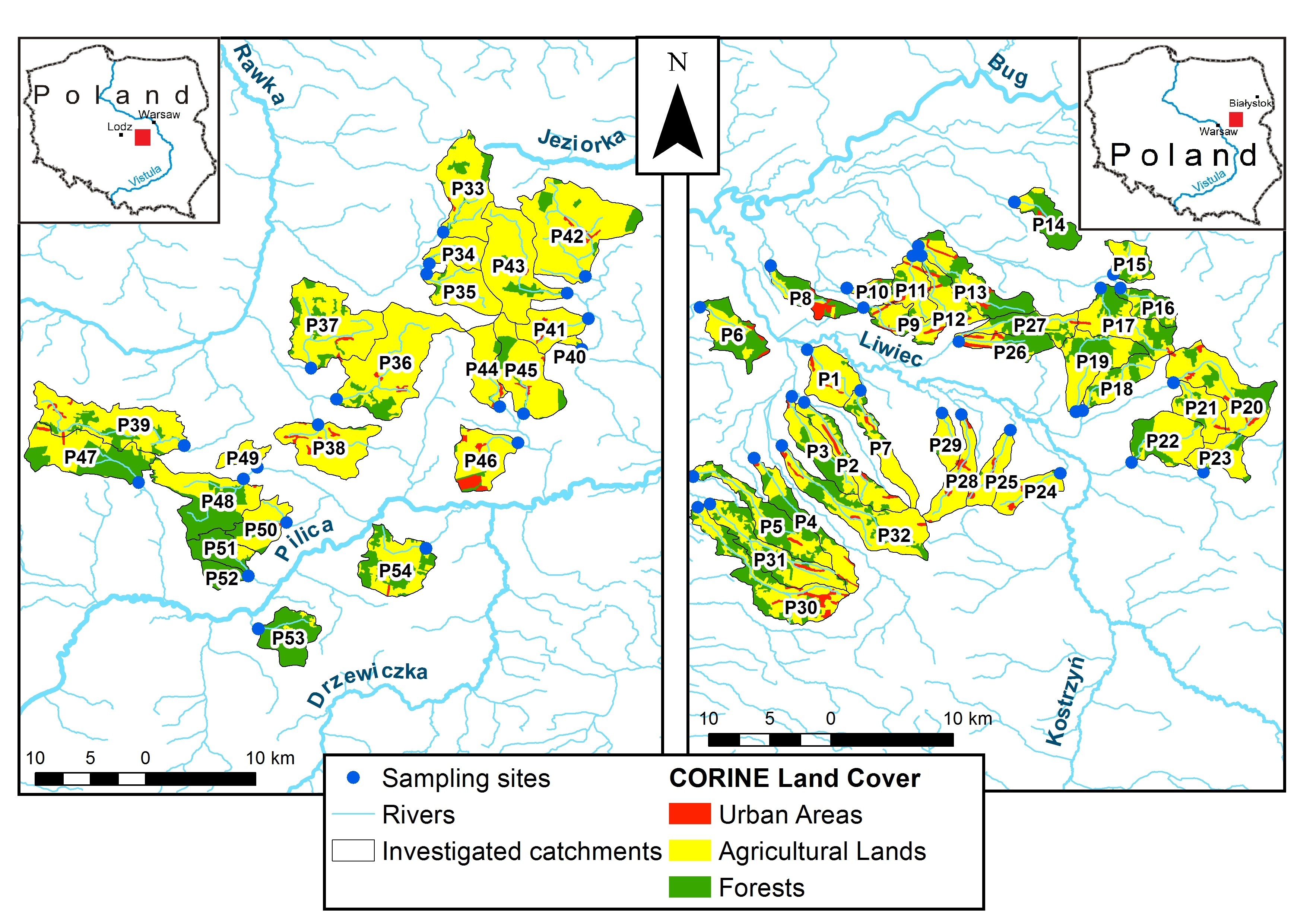
The research was conducted across small lowland streams belonging to the Bug, Narew, Pilica, and Bzura rivers, being major tributaries of the Vistula River in central Poland (Figure 1). The investigated catchments are distributed across the Central Masovia Lowland, the Southern Podlasie Lowland, and the Southern Masovia Hills [49], and built mainly from glacial clays and fluvioglacial sands, which arose during the Warthanian glaciation. In some areas, especially in the Southern Masovia Hills, post-glacial hills such as eskers, terminal moraines, and kames are present [50]. According to [51] and their modified Köppen–Geiger climate classification, the studied area belongs to warm-summer humid continental rate climate (Cfb), with dry periods during winter months (December, January, February) and warm, wet periods from June to August. Similar to the majority of monitored Polish lowland rivers, studied streams are characterized by a nival regime, with the highest streamflow rates observed in spring as the result of snowmelt, and the lowest usually occurring during summer and autumn [52]. The studied area is used mainly for agriculture; crops are dominated by potatoes, rye, corn, oat, and triticale [53,54], while in seven catchments in the Southern Masovia Hills, located in the largest orchard region in Poland, the intensive production of apples, cherries, sweet cherries, and pears is observed [55]. Forested areas, growing mainly on fluvioglacial plains, dunes, and plains of eolian cover sands, are composed mainly of scots pines (Pinus sylvestris L.), silver birch (Betula pendula R.), and common oak (Quercus robur L.). In some river valleys, riparian forests are also present, with a dominance of white willows (Salix alba L.), common aspens (Populus tremula L.), and black alders (Alnus glutinosa (L.) Gaertn.). The surveyed area is generally poorly urbanized, as most of the artificial surfaces are villages and rural settlements, with the only small town (Łochów) located in the P8 catchment.
3. Materials and Methods
3.1. Field and Laboratory Investigations
Field investigations were carried out in 54 independent catchments, with the area ranging from 1.49 to 61.02 km2 (Appendix A, Table A1). The sampling sites were selected in order to maximize differences between land cover properties in the whole catchment area, as well as in the proximity of the streams. Additionally, sampling site selection precluded their localization below dam reservoirs, which significantly modify water quality parameters [56,57], as well as below wastewater inflows, which increase nitrate and ammonia ion concentrations [58,59,60]. Sampling was conducted on a monthly time scale, from November 2021 to March 2022, which covered the period with the lack of the instream vegetation, having a direct impact on nutrient uptake and release [61], as well as sediment trapping, where ion accumulation occurs [62]. In the field, electrical conductivity was measured with the use of portable meters Hi991300 and Hi 9811-5 (Hanna Instruments, Inc., Woonsocket, Rhode Island, USA), both regularly calibrated. Simultaneously, water samples were collected into polyethylene bottles, always from the main current of the streams. After transportation to the laboratory and membrane filtration, NH4+, NO3−, and NO2− ion concentrations were measured photometrically with a LF300 spectrophotometer (Slandi Ltd., Michałowice, Poland). Both measurements and water samples were collected a minimum of three days after rainfall events and simultaneously in stable streamflow conditions.
3.2. Land Cover Metrics
To evaluate the impact of landscape on inorganic nitrogen compounds in stream water, the contribution of individual types of land cover (in %) was calculated on the basis of the Corine Land Cover 2018 (CLC 2018) vector land cover map with 100-m resolution and the 10-m high resolution Sentinel 2 Land Cover Map of Europe (S2GLC). An overall data accuracy obtained for S2GLC (86.1% for the whole dataset and 92.9% for Poland) [63] is similar to accuracies estimated for CLC 2018 (92.43 and 92.67% for a two-stage process) [64]. From both datasets, several classes were distinguished using raster and vector processing tools in ArcMap 10.5 (Table 1). They were chosen because of their occurrence in most of the catchments, as well as their unambiguous interpretation in the context of affecting water quality. Marshes, peatbogs, and water bodies were omitted from the analysis due to their sporadic occurrence and, in consequence, their possible disruption of the statistical analysis due to many zeros appearing in the dataset. Each dataset provides a different share of selected land cover classes, which is the most pronounced in the case of meadows: according to CLC 2018, the study area is occupied by meadows in 6.31%, whereas in S2GLC, the contribution of meadows equals 21.37%. Forests (CLC 2018: 30.17%, S2GLC: 33.2%) and arable land (CLC 2018: 45.62%, S2GLC: 37.87%) in both datasets were similarly represented, while orchards cover only 6.6% of the total study area.
The contribution of land cover classes was calculated for different spatial scales, which is a generally common procedure allowing for the search for best landscape predictors [65,66]. Therefore, land cover was computed for the whole catchment area, for 50-, 250-, and 500-m-wide buffer zones extending from the sampling site upstream to the springs, as well as analogous buffer zones extending 1 km upstream (cut buffer zones). Additionally, a 1 km buffer zone created with the geographical center in sampling sites was adopted (reach scale), similar to [48,67].
3.3. Statistical Analysis
The spatial variability and electrical conductivity of inorganic nitrogen compounds—NH4+, NO3−, and NO2−—were presented graphically on the maps. Average values of concentrations for the study period from November to March were visualized for this purpose with the use of the sequential color scale. To determine the similarity of nitrogen compounds between investigated catchments, hierarchical cluster analysis (CA) was used; for this purpose, the Ward agglomeration method with Euclidean distance as a measure of similarity was applied. Cluster analysis was performed for all parameters simultaneously after data standardization, while the optimal number of clusters was designated with the use of the formula given previously by [68].
To evaluate the performance of land cover characteristics in explaining nitrogen compounds variability, as well as to determine the best spatial scale of metrics with respect to different datasets, the correlation analysis was conducted. Initially, water quality data and land cover properties for all spatial scales were checked if they met the assumption of normal distribution. For this purpose, the Shapiro–Wilk goodness of fit test was used, the results of which indicated that most of the land cover metrics do not meet the assumption of normal distribution (p < 0.05). After normalization with the logarithmic function, the distribution was still abnormal, so the Spearman rank correlation coefficient was used, considered as a non-parametric version of the Pearson coefficient, which was applied to link all of the land cover metrics, calculated for the total catchment area, buffer zones, and reach scale representing sampling sites, with mean concentrations of NH4+, NO3−, and NO2− and EC for the study period. A statistically significant threshold of the correlation was assumed at p = 0.05, while the analysis was performed in the Statistica 13.5 software (TIBCO Software Inc., Palo Alto, CA, USA) and presented in tabular form.
The meteorological background during the sampling period was provided using mean monthly air temperature and monthly precipitation sums from meteorological station Warsaw–Okęcie, operated by the Institute of Meteorology and Water Management, National Research Institute, and located centrally between investigated catchments. Such values were compared to the respective mean values from the period of 1993–2022.
4. Results
4.1. Meteorological Background
The sampling period, as indicated by the measurement data from the Warsaw–Okęcie meteorological station, can be classified as relatively warm in comparison to the reference period 1993–2022, when the average air temperature was 1.4 °C higher and reached 2.5 °C. All months were warmer on average except December, which was 1.0 °C colder in relation to the 30-year reference period. The precipitation sum during the sampling period was slightly lower than in the reference period; total precipitation reached 134 mm, which accounted for 86% of the average sum of precipitation calculated for the 1993–2022 reference period (156 mm). The distribution of precipitation was quite unusual–from November to February, the precipitation sum was near or slightly above the long-term average, while March was extremely dry, with a total precipitation sum of only 1.7 mm.
4.2. Spatial Variability of Water Quality Parameters
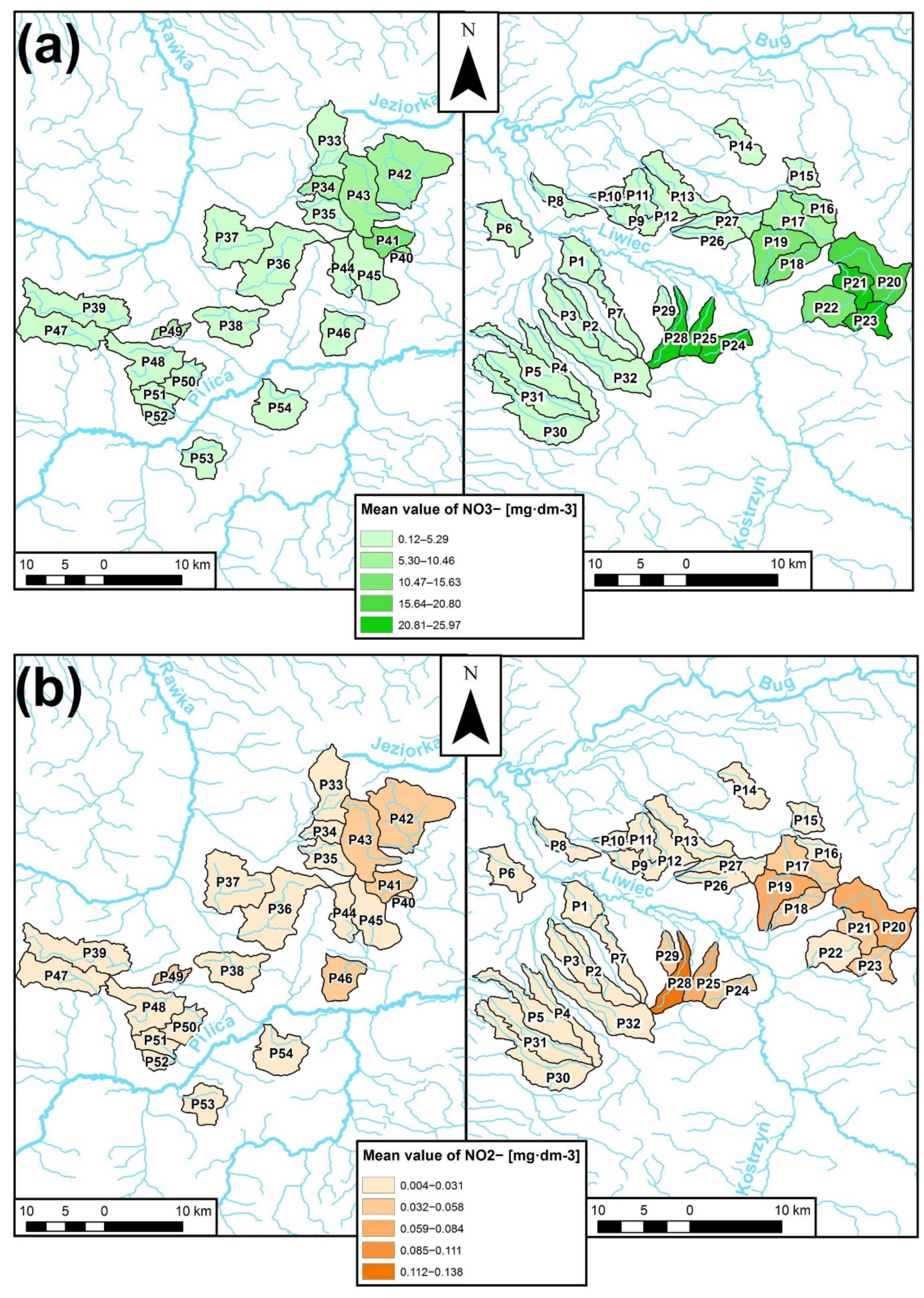
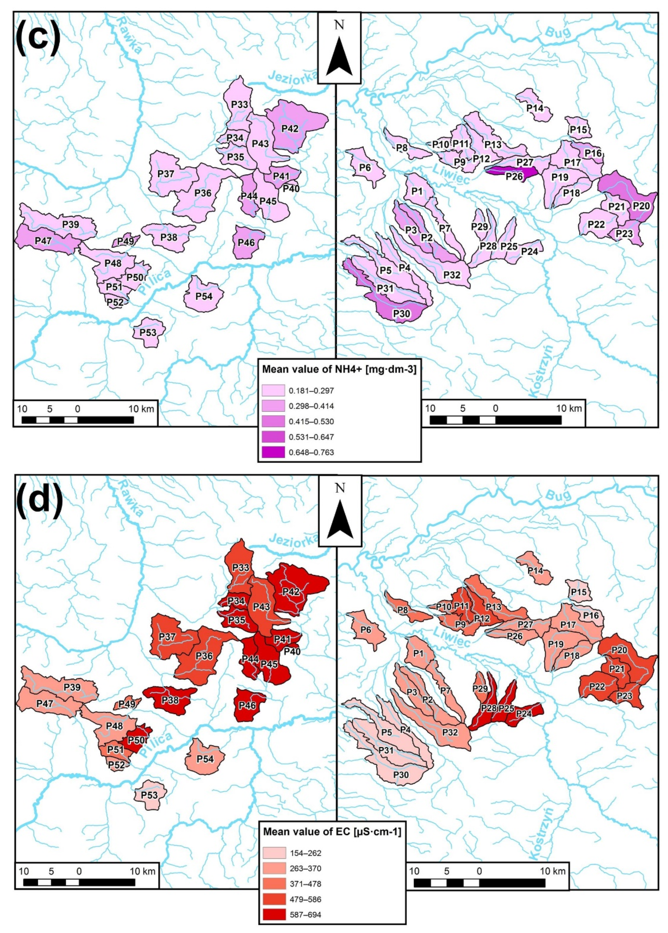
Across the investigated lowland streams, considerable spatial variability of the water quality parameters was documented (Figure 2). Mean nitrates NO3− concentration during the study period reached 5.6 mg·dm−3; in some sampling sites, such as P1, P38, and P53, it did not exceed 1 mg·dm−3, whereas in others belonging to the Bug catchment, the average concentration of NO3− was over 20 mg·dm−3 (P24 and P28) (Figure 2a). The maximum concentration of NO3− during the study period was as high as 48.7 mg·dm−3 in the Korycianka (P28). In the case of the nitrites NO2−, less variability was noted. Their concentrations were more aligned across sampling sites, and simultaneously, their spatial distribution was closely related to NO3− (Figure 2b). In most sites, the concentration of NO2− ions did not exceed 0.01 mg·dm−3, while the average value for all of those investigated was 0.024 mg·dm−3. The maximum concentration, analogous to nitrates, was noted in site P28 and reached 0.185 mg·dm−3. The spatial pattern of the ammonia ion NH4+ concentration was obviously different and did not follow the nitrates and nitrites (Figure 2c). In the majority of the sampling sites, NH4+ concentration was in the range of 0.2–0.5 mg·dm−3, with a mean value of 0.273 mg·dm−3. The site most loaded with NH4+ ions was P26, where in December, the concentration reached even 1.33 mg·dm−3. Electrical conductivity was also clearly varied (Figure 2d), as in some sites, it did not exceed 200 µS·cm−1, while in others, it reached on average over 650 µS·cm−1 (P34, P44, and P45). It must be noted that sampling sites, representing catchments located close to each other, were characterized by similar water quality parameters, which was especially visible in the case of NO3−, NO2−, and EC (Figure 2).
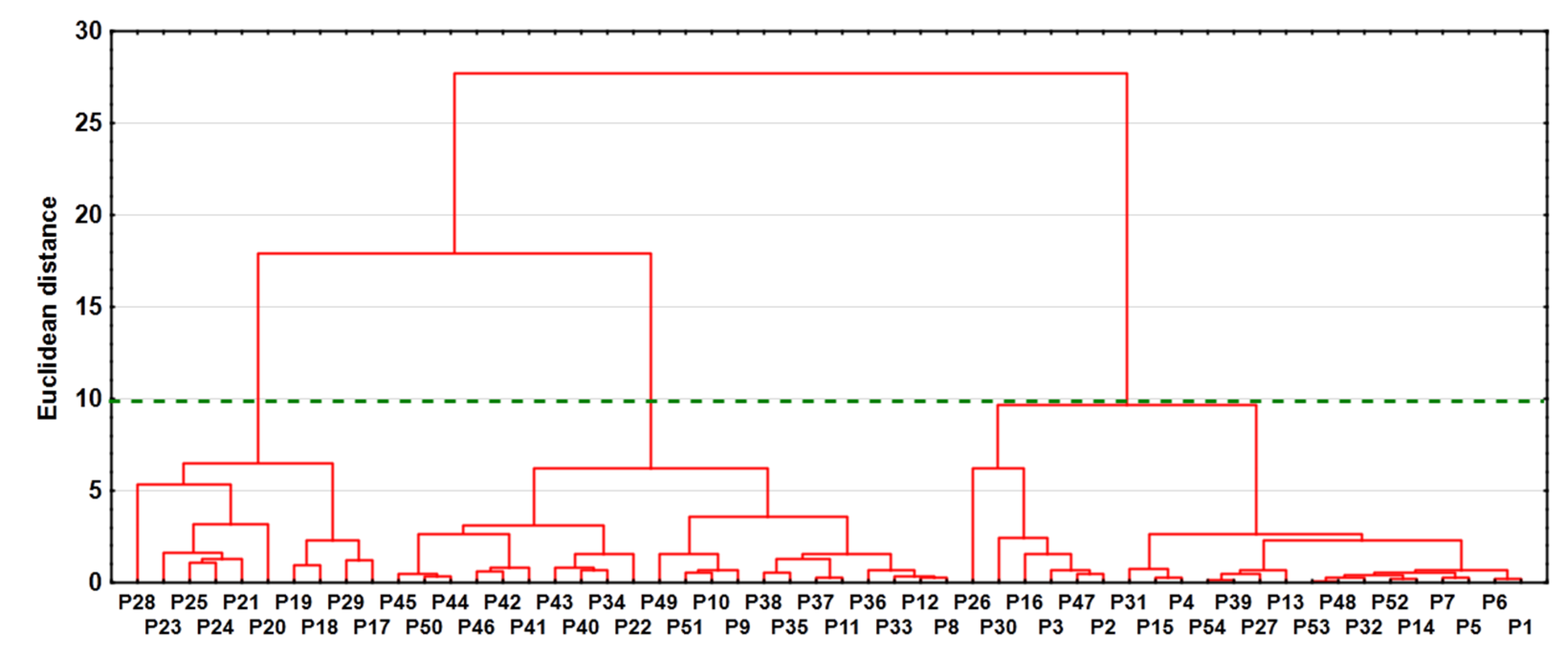
Cluster analysis based on all of the investigated water quality parameters indicated the existence of three main groups (Figure 3). The first cluster linked sites are located mainly in the Southern Masovia Hills (in the Pilica and the Rawka River catchments), characterized by the highest EC value (often above 500 µS·cm−1) and medium-high nitrate and nitrite concentrations. The second cluster indicated nitrate pollution with the highest values of NO3- concentration, as well as above average EC values. The last, third cluster was comprised of sampling sites with small nitrate concentration (usually below 2 mg·dm−3), as well as low values of EC (below 400 µS·cm−1).
4.3. Land Cover Effect on Water Quality
Relationships between land cover metrics and water quality parameters were documented both in the case of CLC 2018 and S2GLC datasets (Table 2 and Table 3). As indicated by correlation analysis, for CLC 2018 data, statistically significant relationships for NO3− and NO2− were captured both for agricultural and forested areas and exhibited a relatively similar pattern. Positive correlations were detected between NO3− and NO2− mean concentrations with arable lands, while negative correlations were observed in the case of meadows and forested areas (Table 2). In the case of forests, only the total forest area metric and coniferous forests were significantly linked with NO3− and NO2− concentrations. In the case of both water quality parameters, there was no relationship with urban areas. A slightly different pattern was found in the case of the EC, which was positively correlated with orchards and urban areas, and negatively with total forest area and coniferous forests. Overall, the best spatial scale for CLC 2018 data was total catchment area and a 500 m wide buffer zone from source to measurement point, which exhibited the best explanatory power. The values of Spearman rank correlation coefficients for narrower buffer zones, radius, and buffer-cropped zones were definitely lower. For ammonia ions NH4+, there was no significant correlation between their concentrations and land cover metrics calculated for all spatial scales (Table 2).
Generally, the S2GLC dataset provided a slightly better correlation performance compared to the respective CLC 2018 dataset (Table 3). In the case of NO3−, NO2−, and EC, it exhibited a similar pattern to CLC 2018; positive correlations were documented in the case of the arable lands, while there were negative correlations with forests, coniferous forests, and meadows. It is important to mention that according to S2GLC, urban areas not only favored increasing EC values, but additionally, their presence resulted in the increase of mean concentrations of NO3− and NO2−. Furthermore, similar to CLC 2018 data, the weakest correlated parameter was ammonia ion NH4+, the mean concentrations of which were positively linked only with deciduous forests and total forests (Table 3). Total catchment area metrics provided the best explanatory power; however, in comparison to CLC 2018, narrower buffer zones (50 m and 250 m wide) played a significant role, with a 500-m cut buffer zone serving as the best spatial scale for meadows.
5. Discussion
5.1. Spatial Variability of the Water Quality Parameters
The study provides unique and extensive insight into the spatial variability of inorganic nitrogen compounds and their landscape dependence in small lowland temperate streams. It must be emphasized that the sampling period was characterized by specific conditions, which potentially may have affected the obtained results. Measurements were conducted from November to March, in a period outside of the growing season, which in Poland lasts on average from 26 March to 7 November [69]. This has a crucial consequence in the context of the nutrient uptake by well-developed macrophytes, algal growth, and terrestrial vegetation [61,70], as well as denitrification [71], which was documented in the spring and summer periods. Thus, in the current investigation, the lack of nutrient uptake resulted in significant variability across the studied sampling sites, especially in the case of the nitrates. However, in comparison to previous studies, the obtained concentrations could be considered as relatively moderate; less contamination from nitrogen compounds was reported in the Pomerania region [72], Warta River [73], and in the Świder River catchment [74], while some catchments had higher concentrations of NO3− and NH4+ [28,75], representing typical agricultural regions. The reason for such moderate NO3− and NH4+ concentrations could be found in hydrometeorological conditions. A lower precipitation sum measured during the sampling period could be responsible for lower concentrations of nitrogen compounds in streams, as it was documented previously by [76,77]. The wetness of the catchment has a strong influence on mobilization and migration, especially involving nitrate ions [4].
5.2. The Effect of Land Cover Characteristics on Selected Nitrogen Compounds Variability
Correlation analysis made it possible to assess the strength and direction of land cover impact on selected water quality parameters. The negative effect of arable lands on nitrogen compound concentrations indicated in this study was also documented in numerous investigations involving this research field conducted in other geographical regions [78,79,80,81], which resulted mainly from the application of organic and mineral fertilizers to areas of cultivation [82]. At the same time, crops usually use less than half of the nitrogen contained in fertilizers; in the case of key crops such as wheat, rice, and maize, the accumulation of the nitrogen contained in fertilizer is less than 40% [83]. During the sampling, conducted outside the vegetation period, the potential for nutrient uptake from fertilizer residues on arable lands was even more limited. In turns, meadows behaved distinctly differently; due to the permanence of plant cover and soil rich in organic matter, meadows are usually a biogeochemical barrier [84,85], which was also reported in this study. It is worth mentioning that the management of such areas is crucial, since meadows may be fertilized, mowed, and grazed, which has an impact on water quality [86].
The impact of woodlands on water quality is more explicit. In the studied area, forests play the role of water purifiers, again in agreement with previous findings [64,87,88,89]. The forest ecosystems are characterized by many nutrient retention mechanisms, from trees and understorey uptake [90] to storage in soil organic matter, which is the largest sink of nitrogen in forests [91,92]. In this research, the results of the correlation analysis, based on CLC 2018 and S2GLC datasets, indicate that forests in general, as well as coniferous forests in particular, have a positive impact on water quality, whereas deciduous forests experienced no impact. According to research conducted by [93] in Europe (climate zones from boreal/north through Atlantic north and sub-Atlantic to Mediterranean/south), coniferous forests are characterized by lower nitrate concentration in soil solutions, which can be affected, among others, by a higher C:N ratio compared to deciduous forests (higher C:N ratio equals lower nitrate leaching). Moreover, in coniferous forests in temperate climate zones, mineralization and nitrification run slow, while in coniferous forests they run clearly faster. The main source of mineral N for coniferous forests is nitrates [90].
The direction of artificial surface impact was clear and it contributed to water quality deterioration, despite the small participation in catchment areas. So far, the negative impact of built-up areas on water quality was confirmed both for urban [94,95] and rural landscapes [96]. In [96], it was indicated that even small settlements have an essential impact on a small waterbody and usually decrease its ecological potential to impermissible limits, mainly due to water enrichment in ammonia nitrogen and total phosphorus. In catchments selected for this study, urban areas (mainly rural settlements) did not contribute to ammonia nitrogen concentration increase, but affected NO3−, NO2−, and EC concentrations. The lack of a relationship between ammonia nitrogen and urban areas may be related to inadequate representation of rural settlements in CLC 2018 and S2GLC, specifically. Incidentally, none of the land use types affect the concentration of that nitrogen compound. In the face of these results, the dominance of rural settlements without a wastewater treatment system in the study area is significant. In some cases, households may be connected with streams and ditches [96], creating point sources of nitrogen that weaken the impact of different land use categories on water quality. This could also be a reason for such spatial variability of the ammonia ions, the average values of which were generally quite uniform in the study period, with the exception of several measurement points.
Finally, it must be emphasized that spatial variability of nitrogen compounds concentrations in streams results not only from land cover configuration and composition, but also from numerous factors not considered in the current study, which cannot be delimited in the catchment borders. It might indeed be related with distinct geographic regions and represent, for example, the degree of sewage system development, nitrogen fertilizer rates in agriculture, waste storage methods, or even socio-economic conditions.
5.3. The Performance of Land Cover Metrics in Different Spatial Scales
The impact of land use and land cover on water quality was considered at different spatial scales. Land cover metrics were previously calculated for the scale of an entire catchment [97,98], subcatchment [77,99], buffer zones of differing width (from 30 m to a few km [66,100]), buffer-cropped zones [101], reach buffers [48,65], and circular buffers [37,102]. Based on previous research on this topic, it is not possible to determine the best spatial scale, in which land use is of the greatest importance for water quality. Many authors claim that land use in the whole catchment is the key to understanding some of the water quality parameters [103,104,105]. There are also results which provide the opposite view, wherein it has been shown that the close vicinity of water bodies can significantly affect nutrient loadings to surface water and influence chemical processes in freshwater ecosystems [65,106,107]. Research conducted by [108] is a link between the two mentioned conclusions; the authors do not indicate a specific spatial scale, as the results do not allow for an unambiguous conclusion. One significant reason for the differences in results may rest in the dissimilarity of the environmental conditions of catchments. Furthermore, [109] stated that the scale and accuracy of spatial data may be one of the main factors influencing such differences. In these contexts, research carried out by [74] provides precious comparability, since it is based on the same spatial datasets with analogous methods and was conducted in similar topographic conditions. Contrary to expectations, it cannot be stated that the results of the mentioned study are corresponding, because one striking difference is the performance of the metrics calculated for forests and arable land at different spatial scales. In the current study, the increase in the spatial scale resulted in the stronger impact of forests on nitrogen compounds and the opposite results were obtained for arable lands; the best performance was found in the case of 250- and 500-m buffer zones. In [74], the most significant with respect to water quality were forests in a narrow buffer zone (100 m) along rivers and arable land in the whole catchment and in the 500-m buffer zone. The source of these inconsistencies may rest in differences in the climatological characteristics of the sampling periods; research conducted in [74] was based on annual measurements during a period of severe drought. In turn, previous studies documented that the impact of land cover on water quality was the most clearly visible in wet periods [110,111] and during floods [112], so this factor could also potentially limit the performance of the obtained correlations in the current study.
Surprisingly, similar results to the current study were obtained on the example of a mountainous region in China; according to [77], the impact of biogeochemical barriers, forests, and meadows was greater at wider spatial scales, whereas the performance of arable land, built-up areas, and bare land was better at smaller spatial scales. So far, it has been emphasized that relatively narrow strips of forests [113] or meadows [85] are able to ensure chemical stability for flowing water ecosystems. In the current study, such a relationship is not clear; moreover, correlation analysis indicates that forests in the narrowest zone may contribute to the enrichment of water with NH4+ ions. Such dependencies and the lack of compliance with the common conviction that biogeochemical barriers in buffer zones are a good tool for protecting waters against pollution may again result from the specificity of the research period. In fact, during the cold period, biogeochemical barriers may lose their functions due to low nutrient uptake and, simultaneously, the decomposition of organic matter (leaf litter) [17] may contribute to the deterioration of water quality.
Finally, it is worth noting that land use at the smallest spatial scales, e.g., in a cut buffer zone and radius, usually had the least impact on the concentration of nitrogen compounds in comparison to buffer zones delineated from springs to sampling points. The weak influence of land cover in smaller scales on water quality are caused by low topographic gradients in lowland catchments; according to [48], such topographic gradients become more pronounced across larger scales, implying that their interactions with water quality normally lie at larger scales.
5.4. Comparison of Land Use Datasets
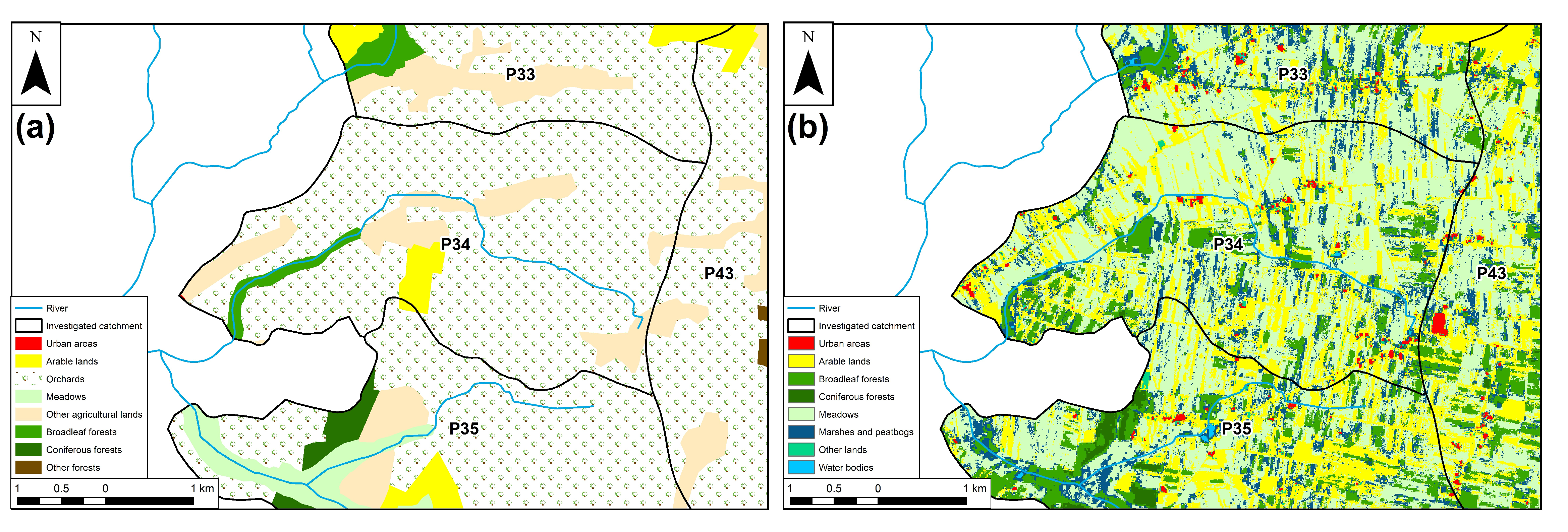
The comparison of two widely available and cost-free land cover datasets, namely CLC 2018 and S2GLC, leads to multiperspective findings. Based only on strength of the relationships measured with Spearman rank correlation coefficients, the S2GLC dataset performed generally better than CLC 2018, giving higher correlations, particularly in the case of the urban areas and arable lands. Furthermore, the number of statistically significant correlations was definitely higher in the case of the S2GLC dataset. It was visible for EC, as well as NO3- and NO2- concentrations and could be documented especially at the smallest spatial scales, such as the 50-m-wide buffer zone, as a result of the higher spatial resolution of the S2GLC dataset [114,115]. Generally, more precise datasets perform visibly better, which was documented on the examples of other research fields, such as agriculture [116] and landscape ecology [117]. Moreover, it is worth noting that the S2GLC dataset does not single out the orchard land cover class, as classification algorithms interpret the majority of orchard areas as meadows or arable lands (Figure 4). According to CLC 2018 data, in six of the investigated catchments (P34, P35, P41, P42, P44, and P45), the contribution of orchards exceeded 70%. This may be a second reason for higher correlation values between NO3−, NO2−, and arable lands for S2GLC, as in orchard catchments, relatively significant nutrient concentrations were documented previously [118], which are more similar in terms of their effects to arable lands than forested areas.
6. Conclusions
In the current study, the influence of land cover on selected water quality parameters was examined regarding the example of 54 catchments, representing the typical Polish lowland landscape in a temperate climate. Overall, in the investigated non-vegetative period, significant spatial variability of NH4+, NO3−, and NO2− ions, as well as electrical conductivity, was documented across sampling sites, which could be mainly related to their catchment land cover. As indicated by correlation analysis both for CLC 2018 and S2GLC datasets, agricultural lands favored higher concentrations of NO3− and NO2−, whereas coniferous forests and meadows reduced nitrogen pollution. In the case of deciduous forests, there was no significant impact on the investigated parameters. In turn, the presence of urbanized (built up) areas increased NO3− and NO2− concentrations, as well as EC values. Significant correlations with land cover metrics were not documented for NH4+ ions, which could be linked to point sources from municipal activity. The study also attempted to search for the best spatial scale of landscape predictors, explaining the spatial variability of selected water quality parameters. The best correlation performance was generally seen for total catchment area and wider buffer zones (250 and 500 m) from springs to sampling sites, while smaller spatial scales, e.g., cut buffer zones and radius, usually had the least impact on the concentration of nitrogen compounds; such a result could be linked to small topographic gradient in lowland catchments. The exceptions were meadows (S2GLC) and orchards (CLC 2018), whose impacts were the greatest in 500-m and 250-m cut buffer zones, respectively. Overall, correlation performance was slightly better in the case of the S2GLC dataset than of the CLC 2018 dataset; however, the differences between datasets in their resolution and class representation must be emphasized. In this context, special attention should be paid to using the best land cover datasets, which should be adjusted to local/regional conditions and in terms of human activities. Finally, the results provide interesting insight into how the water quality depends on factors other than land use, as it was conducted during the period with a lack of significant nutrient uptake and denitrification, followed by the high migration potential of nitrogen compounds. Such an understanding of the relationship between land cover and water quality parameters, based on variable scale metrics and different datasets, seems to be crucial in terms of practical implications related to water management and environmental protection.
Author Contributions
Conceptualization, M.Ł., M.F. and K.S.; methodology, M.Ł., M.F. and K.S.; formal analysis, M.Ł., M.F. and K.S.; investigation, M.Ł., M.F. and K.S.; resources, M.Ł., M.F. and K.S.; writing—original draft preparation, M.Ł., M.F. and K.S.; writing—review and editing, M.Ł., M.F. and K.S.; visualization, M.Ł., M.F. and K.S.; supervision, M.Ł., M.F. and K.S.; project administration, M.Ł.; funding acquisition, M.Ł. All authors have read and agreed to the published version of the manuscript.
Funding
This research was funded by the University of Warsaw, grant number BOB-661-453/2021, and by the Faculty of Geography and Regional Studies, grant number SWIB 53/2021.
Data Availability Statement
Not applicable.
Acknowledgments
The authors would like to express their gratitude to Stanisław Fedorczyk, Monika Kosińska, Paulina Maciejewska, Wiktoria Malinowska, and Katarzyna Sosnowska for the field and laboratory assistance. The authors also thank the two anonymous reviewers for their constructive comments.
Conflicts of Interest
The authors declare no conflict of interest.
Appendix A

Table A1.
Detailed characteristics of catchments in terms of selected land cover types contribution. Abbreviations: A—catchment area [km2], UA—urban areas [%], ARA—arable lands [%], ORCH—orchards [%], MEAD—meadows [%], DF—deciduous forests [%], CF—coniferous forests [%], TF—total forests [%], CLC 2018—Corine Land Cover 2018, S2GLC—Sentinel 2 Global Land Cover.
| Stream | Site | A | CLC 2018 Dataset | S2GLC Dataset | |||||||||||
|---|---|---|---|---|---|---|---|---|---|---|---|---|---|---|---|
| UA | ARA | ORCH | MEAD | CF | DF | TF | UA | ARA | MEAD | CF | DF | TF | |||
| Myszadła Stream | P1 | 15.5 | 4.8 | 61.4 | 0.0 | 22.0 | 0.0 | 1.3 | 1.7 | 0.2 | 27.3 | 52.0 | 3.4 | 11.5 | 14.9 |
| Józefów Stream | P2 | 15.9 | 8.2 | 65.3 | 0.0 | 8.0 | 1.8 | 8.1 | 15.8 | 0.3 | 39.7 | 36.1 | 8.0 | 11.3 | 19.3 |
| Rozalin Stream | P3 | 15.1 | 1.1 | 58.8 | 0.0 | 2.3 | 0.0 | 31.7 | 32.5 | 0.1 | 23.5 | 28.8 | 26.5 | 14.7 | 41.1 |
| Kobylanka | P4 | 17.1 | 3.3 | 52.3 | 0.0 | 1.6 | 0.0 | 30.1 | 42.6 | 0.0 | 18.9 | 25.5 | 32.4 | 12.3 | 44.7 |
| Rynia | P5 | 23.7 | 1.3 | 30.3 | 0.0 | 6.9 | 0.0 | 37.1 | 52.1 | 0.1 | 18.2 | 17.5 | 41.8 | 11.9 | 53.6 |
| Kukawki Stream | P6 | 16.6 | 3.6 | 10.8 | 0.0 | 15.3 | 0.0 | 41.2 | 55.2 | 0.2 | 7.6 | 23.5 | 44.5 | 14.9 | 59.5 |
| Moszczona | P7 | 13.2 | 2.5 | 64.9 | 0.0 | 4.2 | 4.3 | 14.7 | 19.1 | 0.1 | 44.4 | 29.9 | 11.0 | 10.6 | 21.6 |
| Łochów Stream | P8 | 11.4 | 24.1 | 21.8 | 0.0 | 6.9 | 8.5 | 13.2 | 47.2 | 7.3 | 12.3 | 17.6 | 25.2 | 25.9 | 51.1 |
| Łojewski Rów | P9 | 12.3 | 9.5 | 62.6 | 0.0 | 0.0 | 0.0 | 0.0 | 17.9 | 0.4 | 19.4 | 37.1 | 6.7 | 26.3 | 33.1 |
| Ostrówek Stream | P10 | 5.1 | 8.4 | 23.0 | 0.0 | 0.0 | 28.6 | 0.0 | 48.8 | 0.4 | 13.3 | 21.8 | 18.7 | 32.8 | 51.4 |
| Wieliczna Stream | P11 | 12.6 | 6.6 | 56.1 | 0.0 | 8.8 | 3.7 | 0.0 | 18.4 | 0.2 | 18.9 | 46.3 | 4.1 | 23.1 | 27.2 |
| Zgrzebichy Stream | P12 | 12.6 | 7.3 | 44.6 | 0.0 | 15.6 | 2.5 | 6.4 | 15.5 | 0.2 | 24.6 | 41.2 | 7.0 | 21.5 | 28.4 |
| Dzięciołek | P13 | 21.2 | 5.3 | 23.6 | 0.0 | 15.2 | 14.6 | 15.1 | 47.2 | 0.4 | 17.8 | 28.2 | 27.0 | 22.1 | 49.1 |
| Bojewka | P14 | 12.6 | 4.4 | 10.9 | 0.0 | 2.9 | 5.5 | 43.4 | 79.6 | 0.0 | 7.7 | 14.5 | 49.2 | 21.5 | 70.6 |
| Ugoszcz | P15 | 9.8 | 0.0 | 34.6 | 0.0 | 21.7 | 0.0 | 31.2 | 31.2 | 0.0 | 25.7 | 29.1 | 23.8 | 16.8 | 40.6 |
| Chruszczewek Stream | P16 | 9.4 | 0.0 | 25.5 | 0.0 | 0.0 | 4.3 | 52.6 | 74.4 | 0.0 | 17.2 | 6.1 | 42.2 | 29.0 | 71.1 |
| Wrotnów Stream | P17 | 22.6 | 1.6 | 45.5 | 0.0 | 2.6 | 0.0 | 28.2 | 39.6 | 0.1 | 40.4 | 16.1 | 23.0 | 17.2 | 40.2 |
| Kolonia Miedzna Stream | P18 | 12.4 | 0.0 | 61.8 | 0.0 | 0.0 | 0.0 | 18.1 | 30.9 | 0.1 | 46.4 | 18.1 | 17.3 | 16.1 | 33.4 |
| Międzylesie Stream | P19 | 21.8 | 0.0 | 47.8 | 0.0 | 9.1 | 0.0 | 15.0 | 32.6 | 0.1 | 43.5 | 19.0 | 17.7 | 17.0 | 34.7 |
| Miedzanka | P20 | 30.8 | 4.7 | 59.1 | 0.0 | 9.4 | 9.3 | 4.2 | 24.4 | 0.3 | 53.7 | 17.3 | 5.9 | 19.5 | 25.4 |
| Wola Orzeszowska Stream | P21 | 12.8 | 3.6 | 70.4 | 0.0 | 5.4 | 0.0 | 10.0 | 10.0 | 0.2 | 66.2 | 14.4 | 6.1 | 10.5 | 16.7 |
| Jartypor Stream | P22 | 20.0 | 2.9 | 57.9 | 0.0 | 2.2 | 6.3 | 25.3 | 31.6 | 0.1 | 55.6 | 7.9 | 18.0 | 15.2 | 33.3 |
| Chmielów Stream | P23 | 11.9 | 2.3 | 66.6 | 0.0 | 0.0 | 8.9 | 6.4 | 17.1 | 0.4 | 65.1 | 5.6 | 6.1 | 18.9 | 25.0 |
| Zawady Stream | P24 | 10.7 | 5.0 | 80.5 | 0.0 | 9.0 | 0.6 | 2.5 | 3.1 | 0.3 | 69.6 | 22.0 | 1.7 | 4.7 | 6.4 |
| Zalesie Stream | P25 | 11.2 | 8.9 | 90.5 | 0.0 | 0.0 | 0.6 | 0.0 | 0.6 | 0.4 | 71.5 | 22.0 | 0.0 | 4.4 | 4.4 |
| Majdan Stream | P26 | 11.1 | 12.4 | 20.9 | 0.0 | 10.6 | 23.5 | 7.1 | 55.2 | 0.1 | 19.5 | 20.5 | 22.1 | 33.9 | 56.0 |
| Lubicza | P27 | 14.2 | 1.8 | 31.9 | 0.0 | 10.6 | 13.1 | 1.9 | 51.8 | 0.0 | 26.7 | 19.7 | 25.1 | 24.0 | 49.1 |
| Korycianka | P28 | 14.8 | 7.8 | 86.3 | 0.0 | 4.6 | 1.2 | 0.2 | 1.3 | 0.6 | 79.2 | 13.4 | 0.3 | 4.5 | 4.8 |
| Komory Stream | P29 | 7.2 | 1.0 | 84.5 | 0.0 | 4.4 | 3.2 | 0.0 | 3.2 | 0.5 | 58.6 | 31.0 | 0.9 | 6.5 | 7.4 |
| Borucza | P30 | 32.0 | 8.1 | 34.9 | 0.0 | 9.2 | 0.0 | 25.5 | 37.7 | 0.8 | 19.2 | 22.5 | 25.5 | 17.6 | 43.2 |
| Cienka | P31 | 25.0 | 2.7 | 42.4 | 0.0 | 6.8 | 0.0 | 36.0 | 40.4 | 0.0 | 17.2 | 22.5 | 33.8 | 13.8 | 47.6 |
| Pniewniczanka | P32 | 32.6 | 4.2 | 59.6 | 0.0 | 7.0 | 2.8 | 16.9 | 25.1 | 0.2 | 39.9 | 22.5 | 16.5 | 13.9 | 30.4 |
| Białka | P33 | 34.9 | 0.5 | 35.3 | 38.5 | 0.0 | 3.5 | 2.6 | 13.6 | 0.4 | 30.6 | 39.2 | 2.2 | 18.2 | 20.4 |
| Stanisławów Stream | P34 | 12.1 | 0.0 | 2.2 | 83.9 | 0.0 | 2.3 | 0.0 | 2.3 | 0.9 | 24.1 | 53.3 | 0.2 | 9.3 | 9.5 |
| Chodnów Stream | P35 | 20.2 | 0.0 | 2.9 | 77.5 | 7.0 | 0.0 | 3.9 | 3.9 | 0.8 | 28.6 | 40.3 | 2.8 | 14.3 | 17.1 |
| Rylka | P36 | 57.2 | 1.3 | 49.0 | 19.7 | 9.9 | 4.2 | 1.7 | 9.5 | 0.3 | 46.4 | 30.7 | 4.0 | 9.2 | 13.2 |
| Regnów Stream | P37 | 47.7 | 1.2 | 59.0 | 7.9 | 5.0 | 2.6 | 9.6 | 14.1 | 0.5 | 51.8 | 25.9 | 7.4 | 7.9 | 15.3 |
| Strzałki Stream | P38 | 30.5 | 5.3 | 71.2 | 0.9 | 12.9 | 0.0 | 0.1 | 1.1 | 0.2 | 76.1 | 14.4 | 0.8 | 3.2 | 4.0 |
| Krzemionka | P39 | 45.0 | 1.9 | 65.7 | 0.9 | 2.8 | 4.3 | 11.2 | 17.3 | 0.1 | 67.5 | 7.8 | 13.1 | 6.1 | 19.2 |
| Dańków Stream | P40 | 1.5 | 0.0 | 77.3 | 3.8 | 0.0 | 11.2 | 0.0 | 11.2 | 0.2 | 81.6 | 5.8 | 0.0 | 8.9 | 8.9 |
| Huta Błędowska Stream | P41 | 16.4 | 5.5 | 2.0 | 84.6 | 0.0 | 0.0 | 0.0 | 0.0 | 1.4 | 24.4 | 43.1 | 0.5 | 16.6 | 17.1 |
| Machnatka | P42 | 61.0 | 1.3 | 3.8 | 76.7 | 1.6 | 0.0 | 2.7 | 8.2 | 0.9 | 24.4 | 40.4 | 2.3 | 22.9 | 25.2 |
| Mogielanka | P43 | 44.5 | 0.6 | 10.9 | 67.5 | 0.6 | 4.5 | 2.6 | 9.3 | 1.1 | 25.5 | 39.5 | 2.2 | 21.5 | 23.7 |
| Trębaczew Stream | P44 | 17.4 | 2.9 | 0.0 | 78.1 | 1.9 | 1.9 | 0.0 | 6.2 | 0.6 | 27.8 | 42.6 | 0.5 | 14.2 | 14.7 |
| Gostomka | P45 | 33.5 | 1.4 | 2.9 | 73.7 | 0.0 | 1.9 | 5.6 | 14.6 | 0.7 | 24.3 | 34.6 | 2.0 | 22.1 | 24.1 |
| Rosocha Stream | P46 | 23.4 | 13.9 | 50.5 | 19.0 | 2.6 | 0.0 | 0.6 | 5.3 | 0.7 | 34.8 | 38.4 | 1.7 | 10.0 | 11.7 |
| Gać | P47 | 36.7 | 1.3 | 38.2 | 0.0 | 0.7 | 7.4 | 34.0 | 55.2 | 0.1 | 41.0 | 3.0 | 39.5 | 12.2 | 51.6 |
| Luboczanka | P48 | 36.5 | 0.2 | 37.7 | 0.2 | 1.2 | 8.2 | 31.4 | 55.5 | 0.2 | 39.0 | 5.3 | 42.3 | 9.4 | 51.7 |
| Kanice Stream | P49 | 6.8 | 0.4 | 72.7 | 0.0 | 0.0 | 0.0 | 18.6 | 20.7 | 0.0 | 73.1 | 5.2 | 14.9 | 4.2 | 19.0 |
| Rzeczyca | P50 | 16.7 | 2.4 | 54.1 | 0.0 | 5.9 | 0.0 | 12.8 | 21.3 | 0.5 | 62.0 | 11.5 | 16.5 | 4.3 | 20.8 |
| Olszówka | P51 | 13.5 | 0.0 | 8.2 | 0.0 | 0.0 | 8.5 | 59.7 | 88.5 | 0.0 | 7.0 | 4.4 | 72.8 | 10.5 | 83.3 |
| Liciążna Stream | P52 | 7.3 | 0.0 | 2.0 | 0.0 | 0.0 | 0.0 | 83.1 | 94.9 | 0.0 | 2.5 | 3.9 | 81.9 | 6.5 | 88.4 |
| Cetenka | P53 | 19.8 | 0.0 | 3.4 | 0.0 | 1.4 | 5.7 | 70.1 | 95.2 | 0.0 | 3.5 | 2.6 | 77.8 | 9.7 | 87.4 |
| Kiełcznica | P54 | 30.2 | 0.7 | 26.3 | 0.0 | 24.2 | 5.5 | 32.1 | 42.9 | 0.0 | 23.4 | 28.8 | 32.5 | 9.2 | 41.7 |
References
- Meteo-Sagasta, J.; Marjani, S.; Turral, H. Water Pollution from Agriculture: A Global Review. Executive Summary, 1st ed.; FAO and IWMI: Rome, Italy, 2017. [Google Scholar]
- Evans, A.E.; Mateo-Sagasta, J.; Qadir, M.; Boelee, E.; Ippolito, A. Agricultural water pollution: Key knowledge gaps and research needs. Curr. Opin. Environ. Sustain. 2019, 36, 20–27. [Google Scholar] [CrossRef]
- Vörösmarty, C.J.; McIntyre, P.B.; Gessner, M.O.; Dudgeon, D.; Prusevich, A.; Green, P.; Glidden, S.; Bunn, S.E.; Sullivan, C.A.; Liermann, C.R.; et al. Global threats to human water security and river biodiversity. Nature 2010, 467, 555–561. [Google Scholar] [CrossRef] [PubMed] [Green Version]
- Lintern, A.; Webb, J.; Ryu, D.; Liu, S.; Bende-Michl, U.; Waters, D.; Leahy, P.; Wilson, P.; Western, A.W. Key factors influencing differences in stream water quality across space. WIREs Water 2018, 5, e1260. [Google Scholar] [CrossRef] [Green Version]
- Kristensen, P.; Whalley, C.; Zal, F.N.N.; Christiansen, T. European Waters Assessment of Status and Pressures 2018, 1st ed.; EEA: Copenhagen, Denmark, 2018. [Google Scholar]
- Schwarzenbach, R.P.; Egli, T.; Hofstetter, T.B.; Von Gunten, U.V.; Wehrli, B. Global Water Pollution and Human Health. Annu. Rev. Environ. Resour. 2010, 35, 109–136. [Google Scholar] [CrossRef]
- Jayaswal, K.; Sahu, V.; Gurjar, B.R. Water Pollution, Human Health and Remediation. In Water Remediation; Springer: Singapore, 2018; pp. 11–27. [Google Scholar] [CrossRef]
- Scanlon, B.R.; Jolly, I.; Sophocleous, M.; Zhang, L. Global impacts of conversions from natural to agricultural ecosystems on water resources: Quantity versus quality. Water Resour. Res. 2007, 43, W03437. [Google Scholar] [CrossRef] [Green Version]
- Khan, M.N.; Mohammad, F. Eutrophication: Challenges and solutions. In Eutrophication: Causes, Consequences and Control, 1st ed.; Ansari, A.A., Gill, S.S., Eds.; Springer: Singapore, 2014; Volume 2, pp. 1–15. [Google Scholar] [CrossRef]
- Miller, J.D.; Stewart, E.; Hess, T.; Brewer, T. Evaluating landscape metrics for characterising hydrological response to storm events in urbanised catchments. Urban Water J. 2020, 17, 247–258. [Google Scholar] [CrossRef]
- A Snapshot of the World’s Water Quality: Towards a Global Assessment; UNEP: Nairobi, Kenya, 2016; Available online: https://wesr.unep.org/media/docs/assessments/unep_wwqa_report_web.pdf (accessed on 4 September 2022).
- Makarigakis, A.K.; Jimenez-Cisneros, B.E. UNESCO’s Contribution to Face Global Water Challenges. Water 2019, 11, 388. [Google Scholar] [CrossRef] [Green Version]
- WWAP (United Nations World Water Assessment Programme). The United Nations World Water Development Report 2015: Water for Sustainable World; UNESCO: Paris, France, 2015; Available online: https://sustainabledevelopment.un.org/content/documents/1711Water%20for%20a%20Sustainable%20World.pdf (accessed on 4 September 2022).
- Withers, P.J.A.; Neal, C.; Jarvie, H.P.; Doody, D.G. Agriculture and Eutrophication: Where Do We Go from Here? Sustainability 2014, 6, 5853–5875. [Google Scholar] [CrossRef]
- Jiang, Y. China’s water scarcity. J. Environ. Manag. 2009, 90, 3185–3196. [Google Scholar] [CrossRef]
- Starkloff, T. Winter hydrology and soil erosion processes in an agricultural catchment in Norway. Ph.D. Thesis, Wageningen University, Wageningen, The Netherlands, 2017. [Google Scholar] [CrossRef] [Green Version]
- Duan, S.; Delaney-Newcomb, K.; Kaushal, S.S.; Findlay, S.E.G.; Belt, K.T. Potential effects of leaf litter on water quality in urban watersheds. Biogeochemistry 2014, 121, 61–80. [Google Scholar] [CrossRef]
- Kronvang, B.; Jeppesen, E.; Conley, D.J.; Søndergaard, M.; Larsen, S.E.; Ovesen, N.B.; Carstensen, J. Nutrient pressures and ecological responses to nutrient loading reductions in Danish streams, lakes and coastal waters. J. Hydrol. 2005, 304, 274–288. [Google Scholar] [CrossRef]
- Seitzinger, S. Nitrogen cycle: Out of Reach. Nature 2008, 452, 162–163. [Google Scholar] [CrossRef] [PubMed]
- Chislock, M.F.; Doster, E.; Zitomer, R.A.; Wilson, A.E. Eutrophication: Causes, consequences, and controls in aquatic ecosystems. Nat. Educ. Knowl. 2013, 4, 10. [Google Scholar]
- Diaz, R.J.; Rosenberg, R. Spreading Dead Zones and Consequences for Marine Ecosystems. Science 2008, 321, 926–929. [Google Scholar] [CrossRef]
- Giri, S.; Qiu, Z. Understanding the relationship of land uses and water quality in Twenty First Century: A review. J. Environ. Manag. 2016, 173, 41–48. [Google Scholar] [CrossRef] [Green Version]
- Huang, J.; Zhan, J.; Yan, H.; Wu, F.; Deng, X. Evaluation of the Impacts of Land Use on Water Quality: A Case Study in The Chaohu Lake Basin. Sci. World J. 2013, 2013, 329187. [Google Scholar] [CrossRef] [Green Version]
- Guo, M.; Zhou, X.; Li, J.; Wu, W.; Chen, Y. Assessment of the salinization processes in the largest inland freshwater lake of China. Stoch. Environ. Res. Risk Assess. 2015, 33, 89–104. [Google Scholar] [CrossRef]
- Cui, H.; Zhou, X.; Guo, M.; Wu, W. Land use change and its effects on water quality in typical inland lake of arid area in China. J. Environ. Biol. 2016, 37, 603–609. [Google Scholar]
- Gossweiler, B.; Wesström, I.; Messing, I.; Romero, A.M.; Joel, A. Spatial and Temporal Variations in Water Quality and Land Use in a Semi-Arid Catchment in Bolivia. Water 2019, 11, 2227. [Google Scholar] [CrossRef]
- Mararakanye, N.; Le Roux, J.; Franke, A. Long-term water quality assessments under changing land use in a large semi-arid catchment in South Africa. Sci. Total Environ. 2022, 818, 151670. [Google Scholar] [CrossRef]
- Lawniczak, A.E.; Zbierska, J.; Nowak, B.; Achtenberg, K.; Grześkowiak, A.; Kanas, K. Impact of agriculture and land use on nitrate contamination in groundwater and running waters in central-west Poland. Environ. Monit. Assess. 2016, 188, 172. [Google Scholar] [CrossRef] [PubMed] [Green Version]
- Kändler, M.; Blechinger, K.; Seidler, C.; Pavlů, V.; Šandac, M.; Dostálc, T.; Krásac, J.; Vitvarc, T.; Štichc, M. Impact of land use on water quality in the upper Nisa catchment in the Czech Republic and in Germany. Sci. Total Environ. 2017, 586, 1316–1325. [Google Scholar] [CrossRef] [PubMed]
- Clark, K.E.; Bravo, V.D.; Giddings, S.N.; Davis, K.A.; Pawlak, G.; Torres, M.A.; Adelson, A.E.; César-Ávila, C.I.; Boza, X.; Collin, R. Land Use and Land Cover Shape River Water Quality at a Continental Caribbean Land-Ocean Interface. Front. Water 2022, 4, 737920. [Google Scholar] [CrossRef]
- Schueler, T.R.; Fraley-McNeal, L.; Cappiella, K. Is Impervious Cover Still Important? Review of Recent Research. J. Hydrol. Eng. 2009, 14, 309–315. [Google Scholar] [CrossRef] [Green Version]
- Li, Y.; Liu, K.; Li, L.; Xu, Z. Relationship of land use/cover on water quality in the Liao River basin, China. Procedia Environ. Sci. 2012, 13, 1484–1493. [Google Scholar] [CrossRef] [Green Version]
- Zampella, R.A.; Procopio, N.A.; Lathrop, R.G.; Dow, C.L. Relationship of Land-Use/Land-Cover Patterns and Surface-Water Quality in The Mullica River Basin. JAWRA J. Am. Water Resour. Assoc. 2007, 43, 594–604. [Google Scholar] [CrossRef]
- Liberoff, A.L.; Flaherty, S.; Hualde, P.; Asorey, M.I.G.; Fogel, M.L.; Pascual, M.A. Assessing land use and land cover influence on surface water quality using a parametric weighted distance function. Limnologica 2019, 74, 28–37. [Google Scholar] [CrossRef]
- Uuemaa, E.; Roosaare, J.; Mander, Ü. Landscape metrics as indicators of river water quality at catchment scale. Hydrol. Res. 2007, 38, 125–138. [Google Scholar] [CrossRef]
- Casquin, A.; Dupas, R.; Gu, S.; Couic, E.; Gruau, G.; Durand, P. The influence of landscape spatial configuration on nitrogen and phosphorus exports in agricultural catchments. Landsc. Ecol. 2021, 36, 3383–3399. [Google Scholar] [CrossRef]
- Xu, Q.; Wang, P.; Shu, W.; Ding, M.; Zhang, H. Influence of landscape structures on river water quality at multiple spatial scales: A case study of the Yuan river watershed, China. Ecol. Indic. 2021, 121, 107226. [Google Scholar] [CrossRef]
- Song, M.; Jiang, Y.; Liu, Q.; Tian, Y.; Liu, Y.; Xu, X.; Kang, M. Catchment versus Riparian Buffers: Which Land Use Spatial Scales Have the Greatest Ability to Explain Water Quality Changes in a Typical Temperate Watershed? Water 2021, 13, 1758. [Google Scholar] [CrossRef]
- Matysik, M.; Absalon, D.; Habel, M.; Maerker, M. Surface Water Quality Analysis Using CORINE Data: An Application to Assess Reservoirs in Poland. Remote Sens. 2020, 12, 979. [Google Scholar] [CrossRef] [Green Version]
- Aune-Lundberg, L.; Strand, G.-H. The content and accuracy of the CORINE Land Cover dataset for Norway. Int. J. Appl. Earth Obs. Geoinf. 2021, 96, 102266. [Google Scholar] [CrossRef]
- Hua, A.K. Land Use Land Cover Changes in Detection of Water Quality: A Study Based on Remote Sensing and Multivariate Statistics. J. Environ. Public Health 2017, 2017, 7515130. [Google Scholar] [CrossRef] [Green Version]
- Risal, A.; Parajuli, P.B.; Dash, P.; Ouyang, Y.; Linhoss, A. Sensitivity of hydrology and water quality to variation in land use and land cover data. Agric. Water Manag. 2020, 241, 106366. [Google Scholar] [CrossRef]
- Turner, M.G.; Gardner, R.H. Landscape Ecology in Theory and Practice, 2nd ed.; Springer: New York, NY, USA, 2015. [Google Scholar] [CrossRef]
- Alexander, R.B.; Smith, R.A.; Schwarz, G. Effect of stream channel size on the delivery of nitrogen to the Gulf of Mexico. Nature 2000, 403, 758–761. [Google Scholar] [CrossRef]
- Peterson, B.J.; Wollheim, W.M.; Mulholland, P.J.; Webster, J.R.; Meyer, J.L.; Tank, J.L.; Marti, E.; Bowden, W.B.; Valett, H.M.; Hershey, A.E.; et al. Control of nitrogen export from watersheds by headwater streams. Science 2001, 292, 86–90. [Google Scholar] [CrossRef]
- Ensign, S.H.; Doyle, M.W. Nutrient spiraling in streams and river networks. J. Geophys. Res. Biogeosci. 2006, 111, G04009. [Google Scholar] [CrossRef]
- Staponites, L.R.; Barták, V.; Bílý, M.; Simon, O.P. Performance of landscape composition metrics for predicting water quality in headwater catchments. Sci. Rep. 2019, 9, 14405. [Google Scholar] [CrossRef] [Green Version]
- Lei, C.; Wagner, P.D.; Fohrer, N. Effects of land cover, topography, and soil on stream water quality at multiple spatial and seasonal scales in a German lowland catchment. Ecol. Indic. 2021, 120, 106940. [Google Scholar] [CrossRef]
- Solon, J.; Borzyszkowski, J.; Bidłasik, M.; Richling, A.; Badora, K.; Balon, J.; Brzezińska-Wójcik, T.; Chabudziński, Ł.; Dobrowolski, R.; Grzegorczyk, I.; et al. Physico-geographical mesoregions of Poland: Verification and adjustment of boundaries on the basis of contemporary spatial data. Geogr. Pol. 2018, 91, 143–170. [Google Scholar] [CrossRef]
- Makowska, A. Mapa Geologiczna Polski 1:200,000, Arkusz: Skierniewice; Państwowy Instytut Geologiczny: Warsaw, Poland, 1970. Available online: https://bazadata.pgi.gov.pl/data/mgp200/mapy/edycja1/mgp200A49-edycja1.jpg (accessed on 20 June 2022).
- Beck, H.E.; Zimmermann, N.E.; McVicar, T.R.; Vergopolan, N.; Berg, A.; Wood, E.F. Present and future Köppen-Geiger climate classification maps at 1-km resolution. Sci. Data 2018, 5, 180214. [Google Scholar] [CrossRef] [PubMed] [Green Version]
- Wrzesiński, D. Reżimy rzek Polski. In Hydrologia Polski, 1st ed.; Jokiel, P., Marszelewski, W., Pociask-Karteczka, J., Eds.; PWN: Warsaw, Poland, 2017; pp. 215–221. [Google Scholar]
- Kulikowski, R. Produkcja I Towarowość Rolnictwa W Polsce: Przemiany I Zróżnicowania Przestrzenne Po II Wojnie Światowej; Prace Geograficzne nr 241; IGIPZ PAN: Warsaw, Poland, 2013. [Google Scholar]
- Agencja Restrukturyzacji I Modernizacji Rolnictwa. Powierzchnie Upraw W Gminach. Available online: https://rejestrupraw.arimr.gov.pl/ (accessed on 5 September 2022).
- Wójcik, M.; Traczyk, A. Changes in the Spatial Organisation of Fruit Growing at the Beginning of the 21St Century: The Case of Grójec Poviat (Mazovia Voivodeship, Poland). Quaest. Geogr. 2017, 36, 71–84. [Google Scholar] [CrossRef] [Green Version]
- Rigacci, L.N.; Giorgi, A.D.N.; Vilches, C.S.; Ossana, N.A.; Salibián, A. Effect of a reservoir in the water quality of the Reconquista River, Buenos Aires, Argentina. Environ. Monit. Assess. 2013, 185, 9161–9168. [Google Scholar] [CrossRef] [PubMed]
- Lachhab, A.; Trent, M.M.; Motsko, J. Multimetric approach in the effects of small impoundments on stream water quality: Case study of Faylor and Walker Lakes on Middle Creek, Snyder County, PA. Water Environ. J. 2021, 35, 1007–1017. [Google Scholar] [CrossRef]
- Carey, R.O.; Migliaccio, K. Contribution of Wastewater Treatment Plant Effluents to Nutrient Dynamics in Aquatic Systems: A Review. Environ. Manag. 2009, 44, 205–217. [Google Scholar] [CrossRef]
- Figueroa-Nieves, D.; McDowell, W.H.; Potter, J.D.; Martinez, G.; Ortiz-Zayas, J.R. Effects of Sewage Effluents on Water Quality in Tropical Streams. J. Environ. Qual. 2014, 43, 2053–2063. [Google Scholar] [CrossRef]
- Lenart-Boroń, A.; Wolanin, A.; Jelonkiewicz, E.; Żelazny, M. The effect of anthropogenic pressure shown by microbiological and chemical water quality indicators on the main rivers of Podhale, southern Poland. Environ. Sci. Pollut. Res. 2017, 24, 12938–12948. [Google Scholar] [CrossRef]
- Birgand, F.; Skaggs, R.W.; Chescheir, G.M.; Gilliam, J.W. Nitrogen Removal in Streams of Agricultural Catchments—A Literature Review. Crit. Rev. Environ. Sci. Technol. 2007, 37, 381–487. [Google Scholar] [CrossRef]
- Schulz, M.; Kozerski, H.-P.; Pluntke, T.; Rinke, K. The influence of macrophytes on sedimentation and nutrient retention in the lower River Spree (Germany). Water Res. 2003, 37, 569–578. [Google Scholar] [CrossRef]
- Malinowski, R.; Lewiński, S.; Rybicki, M.; Jenerowicz, M.; Gromny, E.; Krupiński, M.; Wojtkowski, C.; Krupiński, M.; Güntner, S.; Krätzschmar, E. S2GLC Final Report. In Scientific Exploitation of Operational Missions Project; 2019. [Google Scholar]
- Moiret-Guigand, A.; Jaffrain, G. CLC 2018 and CLC change 2012–2018 validation report—Copernicus land monitoring service. In File, SIRS SAS; 2021. [Google Scholar]
- Bhat, S.U.; Khanday, S.A.; Islam, S.T.; Sabha, I. Understanding the spatiotemporal pollution dynamics of highly fragile montane watersheds of Kashmir Himalaya, India. Environ. Pollut. 2021, 286, 117335. [Google Scholar] [CrossRef] [PubMed]
- de Mello, K.; Valente, R.A.; Ribeiro, M.P.; Randhir, T. Effects of forest cover pattern on water quality of low-order streams in an agricultural landscape in the Pirapora river basin, Brazil. Environ. Monit. Assess. 2022, 194, 189. [Google Scholar] [CrossRef] [PubMed]
- Pak, H.Y.; Chuah, C.J.; Yong, E.L.; Snyder, S.A. Effects of land use configuration, seasonality and point source on water quality in a tropical watershed: A case study of the Johor River Basin. Sci. Total Environ. 2021, 780, 146661. [Google Scholar] [CrossRef] [PubMed]
- Łaszewski, M.A. The effect of environmental drivers on summer spatial variability of water temperature in Polish lowland watercourses. Environ. Earth Sci. 2020, 79, 244. [Google Scholar] [CrossRef]
- Tomczyk, A.M.; Szyga-Pluta, K. Variability of thermal and precipitation conditions in the growing season in Poland in the years 1966–2015. Theor. Appl. Climatol. 2019, 135, 1517–1530. [Google Scholar] [CrossRef] [Green Version]
- Desmet, N.; Van Belleghem, S.; Seuntjens, P.; Bouma, T.; Buis, K.; Meire, P. Quantification of the impact of macrophytes on oxygen dynamics and nitrogen retention in a vegetated lowland river. Phys. Chem. Earth Parts A/B/C 2011, 36, 479–489. [Google Scholar] [CrossRef]
- Kanownik, W.; Policht-Latawiec, A. Changeability of Oxygen and Biogenic Indices in Waters Flowing through Areas under Various Anthropopressures. Pol. J. Environ. Stud. 2015, 24, 1633–1640. [Google Scholar] [CrossRef]
- Matej-Łukowicz, K.; Wojciechowska, E.; Nawrot, N.; Dzierzbicka-Głowacka, L.A. Seasonal contributions of nutrients from small urban and agricultural watersheds in northern Poland. PeerJ 2020, 8, e8381. [Google Scholar] [CrossRef]
- Górski, J.; Dragon, K.; Kaczmarek, P.M.J. Nitrate pollution in the Warta River (Poland) between 1958 and 2016: Trends and causes. Environ. Sci. Pollut. Res. 2019, 26, 2038–2046. [Google Scholar] [CrossRef] [Green Version]
- Łaszewski, M.; Fedorczyk, M.; Gołaszewska, S.; Kieliszek, Z.; Maciejewska, P.; Miksa, J.; Zacharkiewicz, W. Land Cover Effects on Selected Nutrient Compounds in Small Lowland Agricultural Catchments. Land 2021, 10, 182. [Google Scholar] [CrossRef]
- Kuczyńska, A.; Jarnuszewski, G.; Nowakowska, M.; Wexler, S.K.; Wiśniowski, Z.; Burczyk, P.; Durkowski, T.; Woźnicka, M. Identifying causes of poor water quality in a Polish agricultural catchment for designing effective and targeted mitigation measures. Sci. Total Environ. 2021, 765, 144125. [Google Scholar] [CrossRef]
- van Vliet, M.; Zwolsman, J. Impact of summer droughts on the water quality of the Meuse river. J. Hydrol. 2008, 353, 1–17. [Google Scholar] [CrossRef]
- Shu, X.; Wang, W.; Zhu, M.; Xu, J.; Tan, X.; Zhang, Q. Impacts of land use and landscape pattern on water quality at multiple spatial scales in a subtropical large river. Ecohydrology 2022, 15, e2398. [Google Scholar] [CrossRef]
- Hill, A. Factors affecting the export of nitrate-nitrogen from drainage basins in southern Ontario. Water Res. 1978, 12, 1045–1057. [Google Scholar] [CrossRef]
- Kebede, W.; Tefera, M.; Habitamu, T.; Alemayehu, T. Impact of Land Cover Change on Water Quality and Stream Flow in Lake Hawassa Watershed of Ethiopia. Agric. Sci. 2014, 5, 647–659. [Google Scholar] [CrossRef] [Green Version]
- Fernandes, A.C.P.; Martins, L.M.D.O.; Pacheco, F.A.L.; Fernandes, L.F.S. The consequences for stream water quality of long-term changes in landscape patterns: Implications for land use management and policies. Land Use Policy 2021, 109, 105679. [Google Scholar] [CrossRef]
- Wang, Y.; Liu, X.; Wang, T.; Zhang, X.; Feng, Y.; Yang, G.; Zhen, W. Relating land-use/land-cover patterns to water quality in watersheds based on the structural equation modeling. CATENA 2021, 206, 105566. [Google Scholar] [CrossRef]
- Fixen, P.; West, F.B. Nitrogen Fertilizers: Meeting Contemporary Challenges. Ambio 2002, 31, 169–176. [Google Scholar] [CrossRef]
- Fowler, D.; Coyle, M.; Skiba, U.; Sutton, M.A.; Cape, J.N.; Reis, S.; Sheppard, L.J.; Jenkins, A.; Grizzetti, B.; Galloway, J.N.; et al. The global nitrogen cycle in the twenty-first century. Philos. Trans. R. Soc. B Biol. Sci. 2013, 368, 20130164. [Google Scholar] [CrossRef] [Green Version]
- Ryszkowski, L.; Bartoszewicz, A.; Kedziora, A. Management of matter fluxes by biogeochemical barriers at the agricultural landscape level⋆. Landsc. Ecol. 1999, 14, 479–492. [Google Scholar] [CrossRef]
- Życzyńska-Bałoniak, I.; Szajdak, L.; Jaskulska, R. Impact of Biogeochemical Barriers on the Migration of Chemical Compounds with the Water of Agricultural Landscape. Pol. J. Environ. Stud. 2005, 14, 671–676. [Google Scholar]
- Ryden, J.C.; Ball, P.R.; Garwood, E.A. Nitrate leaching from grassland. Nature 1984, 311, 50–53. [Google Scholar] [CrossRef]
- Bicalho, S.; Langenbach, T.; Rodrigues, R.; Correia, F.; Hagler, A.; Matallo, M.; Luchini, L. Herbicide distribution in soils of a riparian forest and neighboring sugar cane field. Geoderma 2010, 158, 392–397. [Google Scholar] [CrossRef]
- Ou, Y.; Wang, X.; Wang, L.; Rousseau, A.N. Landscape influences on water quality in riparian buffer zone of drinking water source area, Northern China. Environ. Earth Sci. 2016, 75, 114. [Google Scholar] [CrossRef]
- Fernandes, A.C.P.; Martins, L.M.D.O.; Fernandes, L.F.S.; Cortes, R.M.V.; Pacheco, F.A.L. Effect of landscape metrics on water quality over three decades: A case study of the Ave River basin, Portugal. WIT Trans. Ecol. Environ. 2020, 242, 39–49. [Google Scholar] [CrossRef]
- Gebauer, G.; Zeller, B.; Schmidt, G.; May, C.; Buchmann, N.; Colin-Belgrand, M.; Dambrine, E.; Martin, F.; Schulze, E.-D.; Bottner, P. The fate of 15N-labelled nitrogen inputs to coniferous and broadleaf forests. In Carbon and Nitrogen Cycling in European Forest Ecosystems, 1st ed.; Schulze, E.D., Ed.; Springer: Berlin, Germany, 2000. [Google Scholar] [CrossRef]
- Nadelhoffer, K.; Emmett, B.; Gundersen, P.; Kjønaas, O.J.; Koopmans, C.J.; Schleppi, P.; Tietema, A.; Wright, R.F. Nitrogen deposition makes a minor contribution to carbon sequestration in temperate forests. Nature 1999, 398, 145–148. [Google Scholar] [CrossRef]
- Cronan, C.S. (Ed.) Ecosystem Biogeochemistry. In Element Cycling in the Forest Landscape, 1st ed.; Springer: Berlin/Heidelberg, Germany, 2018; Available online: https://link.springer.com/content/pdf/10.1007/978-3-319-66444-6.pdf (accessed on 5 September 2022).
- Kristensen, H.L.; Gundersen, P.; Callesen, I.; Reinds, G.J. Throughfall Nitrogen Deposition Has Different Impacts on Soil Solution Nitrate Concentration in European Coniferous and Deciduous Forests. Ecosystems 2004, 7, 180–192. [Google Scholar] [CrossRef]
- Paul, M.J.; Meyer, J.L. Streams in the Urban Landscape. Annu. Rev. Ecol. Syst. 2001, 32, 333–365. [Google Scholar] [CrossRef]
- Tu, J. Spatial Variations in the Relationships between Land Use and Water Quality across an Urbanization Gradient in the Watersheds of Northern Georgia, USA. Environ. Manag. 2013, 51, 1–17. [Google Scholar] [CrossRef]
- Lysoviene, J.; Gasiunas, V. The impact of rural settlements on water quality in small rivers and drainage channels. In Environmental Engineering, Proceedings of the International Conference on Environmental Engineering, Vilnius, Lithuania, 19–20 May 2011; Vilnius Gediminas Technical University: Vilnius, Lithuania, 2011. [Google Scholar]
- Delesantro, J.M.; Duncan, J.M.; Riveros-Iregui, D.; Blaszczak, J.R.; Bernhardt, E.S.; Urban, D.L.; Band, L.E. Characterizing and classifying urban watersheds with compositional and structural attributes. Hydrol. Process. 2021, 35, e14339. [Google Scholar] [CrossRef]
- Aalipour, M.; Antczak, E.; Dostál, T.; Amiri, B.J. Influences of Landscape Configuration on River Water Quality. Forests 2022, 13, 222. [Google Scholar] [CrossRef]
- Wang, Y.; Yang, G.; Li, B.; Wang, C.; Su, W. Measuring the zonal responses of nitrogen output to landscape pattern in a flatland with river network: A case study in Taihu Lake Basin, China. Environ. Sci. Pollut. Res. 2022, 29, 34624–34636. [Google Scholar] [CrossRef] [PubMed]
- Xu, S.; Li, S.-L.; Zhong, J.; Li, C. Spatial scale effects of the variable relationships between landscape pattern and water quality: Example from an agricultural karst river basin, Southwestern China. Agric. Ecosyst. Environ. 2020, 300, 106999. [Google Scholar] [CrossRef]
- Schmidt, T.S.; Van Metre, P.C.; Carlisle, D.M. Linking the Agricultural Landscape of the Midwest to Stream Health with Structural Equation Modeling. Environ. Sci. Technol. 2018, 53, 452–462. [Google Scholar] [CrossRef] [PubMed] [Green Version]
- Mwaijengo, G.N.; Msigwa, A.; Njau, K.N.; Brendonck, L.; Vanschoenwinkel, B. Where does land use matter most? Contrasting land use effects on river quality at different spatial scales. Sci. Total Environ. 2020, 715, 134825. [Google Scholar] [CrossRef]
- Nielsen, A.; Trolle, D.; Søndergaard, M.; Lauridsen, T.L.; Bjerring, R.; Olesen, J.E.; Jeppesen, E. Watershed land use effects on lake water quality in Denmark. Ecol. Appl. 2012, 22, 1187–1200. [Google Scholar] [CrossRef]
- Shen, Z.; Hou, X.; Li, W.; Aini, G. Relating landscape characteristics to non-point source pollution in a typical urbanized watershed in the municipality of Beijing. Landsc. Urban Plan. 2014, 123, 96–107. [Google Scholar] [CrossRef]
- Wu, J.; Jin, Y.; Hao, Y.; Lu, J. Identification of the control factors affecting water quality variation at multi-spatial scales in a headwater watershed. Environ. Sci. Pollut. Res. 2021, 28, 11129–11141. [Google Scholar] [CrossRef]
- Carey, R.O.; Migliaccio, K.W.; Li, Y.; Schaffer, B.; Kiker, G.A.; Brown, M.T. Land use disturbance indicators and water quality variability in the Biscayne Bay Watershed, Florida. Ecol. Indic. 2021, 11, 1093–1104. [Google Scholar] [CrossRef]
- Miranda, L.S.; Deilami, K.; Ayoko, G.A.; Egodawatta, P.; Goonetilleke, A. Influence of land use class and configuration on water-sediment partitioning of heavy metals. Sci. Total Environ. 2022, 804, 150116. [Google Scholar] [CrossRef]
- Amiri, B.J.; Nakane, K. Entire catchment and buffer zone approaches to modeling linkage between river water quality and land cover—A case study of Yamaguchi Prefecture, Japan. Chin. Geogr. Sci. 2008, 18, 85–92. [Google Scholar] [CrossRef] [Green Version]
- Sliva, L.; Williams, D.D. Buffer Zone versus Whole Catchment Approaches to Studying Land Use Impact on River Water Quality. Water Res. 2001, 35, 3462–3472. [Google Scholar] [CrossRef]
- Huang, Z.; Han, L.; Zeng, L.; Xiao, W.; Tian, Y. Effects of land use patterns on stream water quality: A case study of a small-scale watershed in the Three Gorges Reservoir Area, China. Environ. Sci. Pollut. Res. 2016, 23, 3943–3955. [Google Scholar] [CrossRef] [PubMed]
- Shi, P.; Zhang, Y.; Li, Z.; Li, P.; Xu, G. Influence of land use and land cover patterns on seasonal water quality at multi-spatial scales. CATENA 2017, 151, 182–190. [Google Scholar] [CrossRef]
- Wang, Y.; Yang, G.; Li, B. Exploring the pivotal response relationship between landscape composition–configuration–intensity metrics and water quality in Taihu basin, China. Ecol. Indic. 2022, 136, 108638. [Google Scholar] [CrossRef]
- Sweeney, B.W.; Newbold, J.D. Streamside Forest Buffer Width Needed to Protect Stream Water Quality, Habitat, and Organisms: A Literature Review. JAWRA J. Am. Water Resour. Assoc. 2014, 50, 560–584. [Google Scholar] [CrossRef]
- Malinowski, R.; Lewiński, S.; Rybicki, M.; Gromny, E.; Jenerowicz, M.; Krupiński, M.; Nowakowski, A.; Wojtkowski, C.; Krupiński, M.; Krätzschmar, E.; et al. Automated Production of a Land Cover/Use Map of Europe Based on Sentinel-2 Imagery. Remote Sens. 2020, 12, 3523. [Google Scholar] [CrossRef]
- Sentinel-2 Global Land Cover. Project Summary. Available online: https://s2glc.cbk.waw.pl/project-summary (accessed on 9 October 2022).
- Pérez-Hoyos, A.; Rembold, F.; Kerdiles, H.; Gallego, J. Comparison of Global Land Cover Datasets for Cropland Monitoring. Remote Sens. 2017, 9, 1118. [Google Scholar] [CrossRef]
- Liu, P.; Pei, J.; Guo, H.; Tian, H.; Fang, H.; Wang, L. Evaluating the Accuracy and Spatial Agreement of Five Global Land Cover Datasets in the Ecologically Vulnerable South China Karst. Remote Sens. 2022, 14, 3090. [Google Scholar] [CrossRef]
- Stępniewski, K.; Łaszewski, M. Spatial and Seasonal Dynamics of Inorganic Nitrogen and Phosphorous Compounds in an Orchard-Dominated Catchment with Anthropogenic Impacts. Sustainability 2021, 13, 11337. [Google Scholar] [CrossRef]
Figure 1.
The localization of investigated catchments on the background of the Corine Land Cover data and drainage system based on a digital hydrographic map of Poland.
Figure 1.
The localization of investigated catchments on the background of the Corine Land Cover data and drainage system based on a digital hydrographic map of Poland.

Figure 2.
The spatial variability of NO3− (a), NO2− (b) and NH4+ (c) concentrations, as well as EC values (d) in the investigated lowland streams.
Figure 2.
The spatial variability of NO3− (a), NO2− (b) and NH4+ (c) concentrations, as well as EC values (d) in the investigated lowland streams.


Figure 3.
Clustering results via the Ward method for all parameters after standardization. The horizontal green dashed line indicates optimal number of clusters.
Figure 3.
Clustering results via the Ward method for all parameters after standardization. The horizontal green dashed line indicates optimal number of clusters.

Figure 4.
A spatial comparison of CLC 2018 (a) and S2GLC (b) datasets regarding the P34 catchment.

Table 1.
CLC 2018 and S2GLC classes used for land cover metric calculations.
| Land Cover Type | CLC 2018 Classes | S2GLC Classes |
|---|---|---|
| Urban areas | All types belonged to class 1. (artificial surfaces) | 1.1.1. Artificial surfaces and constructions |
| Arable lands | 2.1.1. Non-irrigated arable land | 2.1.1. Cultivated areas |
| Orchards | 2.2.2. Fruit trees and berry plantations | - |
| Meadows | 2.3.1. Pastures, meadows, and other permanent grasslands under agricultural use | 2.3.1. Herbaceous vegetation |
| Deciduous forests | 3.1.1. Broad-leaved forest | 3.1.1. Broadleaf tree cover |
| Coniferous forests | 3.1.2. Coniferous forest | 3.1.2. Coniferous tree cover |
| Total forests | Sum of 3.1.1. and 3.1.2. classes | Sum of 3.1.1. and 3.1.2. classes |
Table 2.
Spearman rank correlation coefficients linking selected land cover metrics from Corine Land Cover 2018 and mean NO3−, NO2−, NH4+, EC across investigated lowland streams during the study period. Abbreviations: TCA—total catchment area; BZ: 50 m, 250 m, 500 m—buffer zone width; BCZ: 50 m−1 km, 250 m−1 km, 500 m−1 km—buffer-cropped zone width-length; UA—urban areas, ARA—arable lands, ORCH—orchards, MEAD—meadows, DF—deciduous forests, CF—coniferous forests, and TF—total forests. The bold type indicates a statistically significant correlation at p = 0.05.
| Parameter | Land Cover Type | TCA | BZ 50 m | BZ 250 m | BZ 500 m | BCZ 50 m−1 km | BCZ 250 m−1 km | BCZ 500 m−1 km | Radius 1000 m |
|---|---|---|---|---|---|---|---|---|---|
| NO3− | UA | −0.027 | 0.191 | 0.179 | 0.063 | −0.103 | −0.037 | −0.054 | −0.121 |
| ARA | 0.256 | 0.188 | 0.308 | 0.347 | 0.044 | 0.130 | 0.148 | 0.161 | |
| ORCH | 0.140 | 0.162 | 0.140 | 0.164 | 0.232 | 0.249 | 0.246 | 0.246 | |
| MEAD | −0.365 | −0.185 | −0.303 | −0.354 | −0.229 | −0.268 | −0.315 | −0.300 | |
| DF | −0.055 | −0.186 | −0.158 | −0.137 | −0.081 | −0.132 | −0.175 | −0.165 | |
| CF | −0.355 | −0.099 | −0.200 | −0.222 | −0.011 | −0.062 | −0.047 | −0.131 | |
| TF | −0.407 | −0.153 | −0.212 | −0.282 | −0.004 | −0.054 | −0.109 | −0.152 | |
| NO2− | UA | 0.104 | 0.242 | 0.256 | 0.188 | −0.060 | −0.005 | 0.018 | −0.035 |
| ARA | 0.264 | 0.135 | 0.294 | 0.343 | 0.089 | 0.176 | 0.196 | 0.206 | |
| ORCH | 0.147 | 0.142 | 0.156 | 0.174 | 0.275 | 0.282 | 0.281 | 0.280 | |
| MEAD | −0.305 | −0.150 | −0.268 | −0.314 | −0.182 | −0.227 | −0.268 | −0.250 | |
| DF | −0.057 | −0.173 | −0.141 | −0.121 | −0.092 | −0.139 | −0.184 | −0.174 | |
| CF | −0.489 | −0.257 | −0.353 | −0.371 | −0.105 | −0.216 | −0.206 | −0.286 | |
| TF | −0.479 | −0.237 | −0.293 | −0.367 | −0.096 | −0.196 | −0.255 | −0.304 | |
| NH4+ | UA | 0.142 | 0.199 | 0.177 | 0.184 | 0.047 | 0.108 | 0.095 | 0.021 |
| ARA | −0.256 | −0.226 | −0.194 | −0.195 | −0.120 | −0.138 | −0.157 | −0.152 | |
| ORCH | 0.036 | 0.061 | 0.075 | 0.035 | 0.185 | 0.217 | 0.223 | 0.224 | |
| MEAD | −0.214 | −0.196 | −0.218 | −0.234 | −0.067 | −0.109 | −0.140 | −0.121 | |
| DF | 0.004 | 0.123 | 0.087 | 0.038 | −0.034 | −0.032 | −0.055 | −0.057 | |
| CF | 0.108 | 0.015 | 0.031 | 0.019 | 0.029 | −0.031 | −0.065 | −0.054 | |
| TF | 0.139 | 0.088 | 0.070 | 0.055 | −0.052 | −0.063 | −0.056 | −0.054 | |
| EC | UA | 0.159 | 0.244 | 0.309 | 0.277 | −0.006 | −0.032 | −0.038 | 0.054 |
| ARA | 0.057 | −0.108 | 0.003 | 0.087 | −0.252 | −0.197 | −0.182 | −0.174 | |
| ORCH | 0.583 | 0.511 | 0.594 | 0.620 | 0.497 | 0.570 | 0.568 | 0.570 | |
| MEAD | −0.198 | −0.015 | −0.104 | −0.130 | −0.015 | −0.077 | −0.102 | −0.101 | |
| DF | −0.012 | 0.017 | 0.007 | −0.007 | 0.206 | 0.158 | 0.149 | 0.157 | |
| CF | −0.732 | −0.654 | −0.691 | −0.721 | −0.335 | −0.449 | −0.452 | −0.456 | |
| TF | −0.733 | −0.361 | −0.555 | −0.696 | −0.082 | −0.185 | −0.282 | −0.310 |
Table 3.
Spearman rank correlation coefficients linking selected land cover metrics from the Sentinel−2 Global Land Cover and mean NO3−, NO2−, NH4+, EC across investigated lowland streams during the study period. Abbreviations are the same in comparison with Table 2. The bold type indicates a statistically significant correlation at p = 0.05.
| Parameter | Land Cover Type | TCA | BZ 50 m | BZ 250 m | BZ 500 m | BCZ 50 m−1 km | BCZ 250 m−1 km | BCZ 500 m−1 km | Radius 1000 m |
|---|---|---|---|---|---|---|---|---|---|
| NO3- | UA | 0.312 | 0.319 | 0.391 | 0.371 | 0.198 | 0.209 | 0.325 | 0.214 |
| ARA | 0.461 | 0.652 | 0.610 | 0.556 | 0.262 | 0.129 | 0.467 | 0.435 | |
| MEAD | −0.069 | −0.182 | −0.318 | −0.253 | −0.271 | −0.045 | −0.414 | −0.360 | |
| DF | −0.019 | −0.101 | −0.103 | −0.145 | 0.080 | −0.121 | −0.092 | −0.098 | |
| CF | −0.469 | −0.129 | −0.231 | −0.270 | 0.171 | 0.003 | −0.141 | −0.158 | |
| TF | −0.411 | −0.093 | −0.201 | −0.297 | 0.095 | −0.115 | −0.201 | −0.212 | |
| NO2- | UA | 0.452 | 0.429 | 0.511 | 0.479 | 0.216 | 0.211 | 0.341 | 0.222 |
| ARA | 0.489 | 0.628 | 0.636 | 0.598 | 0.393 | 0.165 | 0.530 | 0.489 | |
| MEAD | −0.001 | −0.127 | −0.253 | −0.186 | −0.229 | 0.062 | −0.354 | −0.290 | |
| DF | −0.024 | −0.094 | −0.084 | −0.121 | −0.004 | −0.157 | −0.148 | −0.175 | |
| CF | −0.566 | −0.225 | −0.301 | −0.385 | 0.141 | −0.078 | −0.283 | −0.307 | |
| TF | −0.472 | −0.129 | −0.250 | −0.364 | 0.018 | −0.201 | −0.279 | −0.309 | |
| NH4+ | UA | 0.172 | 0.222 | 0.135 | 0.162 | 0.143 | −0.142 | 0.122 | −0.012 |
| ARA | −0.188 | −0.164 | −0.143 | −0.132 | −0.061 | −0.146 | −0.080 | −0.096 | |
| MEAD | −0.054 | −0.257 | −0.090 | −0.042 | −0.182 | 0.000 | −0.087 | −0.043 | |
| DF | 0.205 | 0.329 | 0.343 | 0.266 | 0.164 | −0.069 | 0.250 | 0.210 | |
| CF | 0.087 | 0.040 | 0.136 | 0.084 | 0.249 | 0.038 | 0.089 | 0.036 | |
| TF | 0.188 | 0.290 | 0.234 | 0.168 | 0.176 | 0.032 | 0.149 | 0.082 | |
| EC | UA | 0.692 | 0.646 | 0.698 | 0.733 | 0.307 | 0.171 | 0.437 | 0.453 |
| ARA | 0.419 | 0.510 | 0.535 | 0.499 | 0.142 | 0.112 | 0.370 | 0.340 | |
| MEAD | 0.307 | −0.075 | 0.087 | 0.194 | −0.266 | 0.050 | −0.153 | −0.118 | |
| DF | −0.118 | −0.218 | −0.321 | −0.322 | 0.122 | −0.039 | 0.021 | −0.034 | |
| CF | −0.813 | −0.495 | −0.708 | −0.754 | 0.062 | 0.044 | −0.478 | −0.428 | |
| TF | −0.699 | −0.273 | −0.573 | −0.673 | 0.065 | −0.101 | −0.270 | −0.310 |
Publisher’s Note: MDPI stays neutral with regard to jurisdictional claims in published maps and institutional affiliations. |
© 2022 by the authors. Licensee MDPI, Basel, Switzerland. This article is an open access article distributed under the terms and conditions of the Creative Commons Attribution (CC BY) license (https://creativecommons.org/licenses/by/4.0/).
Share and Cite
MDPI and ACS Style
Łaszewski, M.; Fedorczyk, M.; Stępniewski, K. The Impact of Land Cover on Selected Water Quality Parameters in Polish Lowland Streams during the Non-Vegetative Period. Water 2022, 14, 3295. https://doi.org/10.3390/w14203295
AMA Style
Łaszewski M, Fedorczyk M, Stępniewski K. The Impact of Land Cover on Selected Water Quality Parameters in Polish Lowland Streams during the Non-Vegetative Period. Water. 2022; 14(20):3295. https://doi.org/10.3390/w14203295
Chicago/Turabian StyleŁaszewski, Maksym, Michał Fedorczyk, and Krzysztof Stępniewski. 2022. "The Impact of Land Cover on Selected Water Quality Parameters in Polish Lowland Streams during the Non-Vegetative Period" Water 14, no. 20: 3295. https://doi.org/10.3390/w14203295
Note that from the first issue of 2016, this journal uses article numbers instead of page numbers. See further details here.