
Remote Monitoring of NH3-N Content in Small-Sized Inland Waterbody Based on Low and Medium Resolution Multi-Source Remote Sensing Image Fusion
1
School of the Geo-Science & Technology, Zhengzhou University, Zhengzhou 450001, China
2
School of Water Conservancy Science & Engineering, Zhengzhou University, Zhengzhou 450001, China
3
Library of Zhengzhou University, Zhengzhou University, Zhengzhou 450001, China
4
Henan Institute of Regional Geological Survey, Zhengzhou 450001, China
*
Author to whom correspondence should be addressed.
Water 2022, 14(20), 3287; https://doi.org/10.3390/w14203287
Submission received: 16 September 2022
/
Revised: 13 October 2022
/
Accepted: 16 October 2022
/
Published: 18 October 2022
(This article belongs to the Section Water Quality and Contamination)
Abstract
:In applying quantitative remote sensing in water quality monitoring for small inland rivers, the time-frequency of monitoring dramatically impacts the accuracy of time-spatial changes estimates of the water quality parameters. Due to the limitation of satellite sensor design and the influence of atmospheric conditions, the number of spatiotemporal dynamic monitoring images of water quality parameters is insufficient. Meanwhile, MODIS and other high temporal resolution images’ spatial resolution is too low to effectively extract small inland river boundaries. To solve the problem, many researchers used Spatio-temporal fusion models in multisource data remote sensing monitoring of ground features. The wildly used Spatio-temporal fusion models, such as FSDAF (flexible spatial-temporal data fusion), have poor performance in heterogeneous changes of ground objects. We proposed a spatiotemporal fusion algorithm SR-FSDAF (Super-resolution based flexible spatiotemporal data fusion) to solve the problem. Based on the FSDAF, it added ESPCN to reconstruct the spatial change prediction image, so as to obtain better prediction results for heterogeneous changes. Both qualitative and quantitative evaluation results showed that our fusion algorithm obtained better results. We compared the band sensitivity of the images before and after fusion to find out that the sensitive band combination of NH3-N has not changed, which proved that the fusion method can be used to improve the time-frequency of NH3-N inversion. After the fusion, we compared the accuracy of linear regression and random forest inversion models and selected the random forest model with better accuracy to predict the NH3-N concentration. The inversion accuracy of NH3-N was as follows: the R2 was 0.75, the MAPE was 23.7% and the RMSE was 0.15. The overall concentration change trend of NH3-N in the study area was high-water period < water-stable period < low water period. NH3-N pollution was serious in some reaches.
1. Introduction
Water is one of the most important materials on earth. With human industrial production, agricultural breeding, and daily activities, a large amount of sewage is discharged into the surrounding water environment, resulting in environmental pollution and a severe impact on water supply ecology and human health. Monitoring the water quality in time and obtaining the temporal-spatial variation characteristics of regional water pollutant concentration is of great significance for assessing the risk of water pollution and effectively preventing water pollution. Traditional water quality detection methods are costly, time-consuming, and laborious. The pollutant concentration obtained at the sampling point cannot reflect the distribution of pollutants in the whole region. Using remote sensing images can realize regional synchronous observation, obtain the overall distribution of contaminants, and provide timely and reliable prediction results for inland water quality monitoring, which is not available through traditional water quality detection methods.
Water quality monitoring based on remote sensing technology is an important research direction of environmental remote sensing, and NH3-N is a valuable reference index for water pollution prevention and control. The concentration of NH3-N in water is related to water eutrophication and suspended solids [1]. Gong et al. found that the correlation coefficient of nitrogen was the highest at 404 nm and 447 nm [2]. Wang et al. found that NH3-N highly correlated with the red, green, and near-infrared (NIR) bands of the SPOT 5 satellite [3]. Existing studies have shown that the relationship between NH3-N concentration and reflection spectrum is the theoretical basis for applying remote sensing technology in water quality monitoring.
Current satellite data for remote sensing water quality monitoring include MODIS [4,5,6,7], MERIS [8,9], TM/ETM + [10,11], Worldview-2 [12,13], HJ-1 CCD [14,15], GF-1 [16,17], sentinel-2 [18,19], etc. Most of these studies focus on large water bodies such as lakes or offshore, and there are few studies on inland rivers, especially on small and medium-sized rivers. The inland river has higher requirements for the spatial resolution and returns period of the satellite, which is hard to meet with a single satellite sensor. Therefore, it is significant to study hyperspectral and high-resolution image fusion algorithms to improve the images’ spatial and temporal resolution for remote sensing monitoring inland rivers. Many works have used the existing Spatio-temporal fusion model for high-frequency remote sensing monitoring of ground feature changes [20].
The Spatio-temporal fusion algorithm is based on ground features’ spectral changes in the high spatial resolution remote sensing image (MODIS). It fuses these changes into the remote sensing image with a high spatial resolution (OLI) to simulate the image with higher temporal resolution and better spatial resolution, which provides reference and image support for the study of temporal and spatial variations monitoring of surface features. The existing Spatio-temporal fusion algorithms can be classified into five types according to different principles: Spatio-temporal fusion algorithms based on spectral unmixing [21,22,23], algorithms based on weight distribution [24,25,26], Bayesian principle algorithms [27,28], feature learning algorithms [29,30,31], and hybrid methods [32,33,34]. The method based on spectral unmixing uses coarse pixels to estimate the value of fine pixels through spectral mixing theory. Niu et al. proposed STDFA (Spatial-Temporal Data Fusion Approach) based on this method [22]. Unmixing-based methods have huge unmixing errors and lack in-class variation of ground objects. The weight-based algorithms include STARFM (Spatial and Temporal Adaptive Reflectance Fusion Model) [24], ESTARFM (Enhanced Spatial and Temporal Adaptive Reflectance Fusion Model) [26], and STAARCH (Spatial and Temporal Adaptive Algorithm for Mapping Reflectance Changes) [25], etc. Weight-based methods use image information for weight assignment to estimate high-resolution pixel values, are invalid for heterogeneous changes, and the weight function based on experience lacks mobility. The method based on Bayesian estimation theory defines the relationship between the coarse image and the fusing image based on the Bayesian statistical principle, but the function establishment process is complex, and its performance in heterogeneous landscapes is unsatisfactory [35]. For the learning-based method, machine learning is used to simulate the mapping relationship between high-resolution and low-resolution images so as to predict the fused image, such as SPSTFM (Sparse representation based Spatio-temporal Reflectance Fusion Model) proposed by Huang et al. [29]. So far, dictionary pairing learning [29], extreme learning [36], random forest [37], deep convolution neural network [30], and artificial neural network [38] have been used for Spatio-temporal data fusion. Although the fusion results are improved, the learning cost is high, the mobility is poor, and the spectral principle support is lacking support. The hybrid method integrates two or more methods in the first four categories, such as FSDAF (Flexible Spatiotemporal Data Fusion) proposed by Zhu et al., which combines unmixing, weighting function, and spatial interpolation methods to reduce the input of the image and enhance the prediction of heterogeneous changes [32]. However, the performance is still not ideal, and it cannot meet the requirement of higher precision change monitoring.
To improve the poor performance in heterogeneous region prediction, we propose an improved Spatio-temporal data fusion model SR-FSDAF (super-resolution flexible spatiotemporal data fusion). Unlike deep learning techniques, which use high-cost training to enhance the accuracy of image fusion, it maintains the simplicity of FSDAF and uses fewer image pairs and less time. SR-FSDAF inherits the hybrid model of FSDAF and improves the thin-plate spline sampling method based on MODIS spectral information to extract spatial variation details and achieves better reconstruction results consistent with resampling purposes. SR-FSDAF can more accurately predict fine-resolution images of heterogeneous regions. Different from other multi-spectral and high-resolution images, OLI and MODIS were launched earlier and allowed free access to more historical image information. Some bands of MODIS are similar to those of OLI and have the band basis for image fusion. Therefore, SR-FSDAF was tested using MODIS and Landsat-8 OLI images and compared with other fusion methods such as STARFM. Then MODIS images, OLI images, and SR-FSDAF were applied to water quality monitoring in Xinyang City to improve the utilization of monitoring frequency and low-resolution images. The NH3-N inversion model was established based on the fused image band, and the NH3-N concentration in the Huaihe River Basin of the Xinyang area was analyzed. For NH3-N concentration inversion, we compared the accuracy of statistical regression model and random forest model, and adopted random forest model to further improve the accuracy of NH3-N concentration prediction.
2. Materials and Methods
2.1. FSDAF
Zhu et al. proposed FSDAF in 2016 [32]. In the method, fine pixels are classified into different types. Temporal variation values of each type are roughly gained by calculating the changes of different classes of ground objects reflected in the pure pixels of MODIS. The thin plate spline sampling (TPS) is carried out on the MODIS image of the prediction date to obtain the rough spatial variation value of ground objects [39]. TPS interpolates and resamples the data based on spatial correlation to preserve the local change information of the image. The two kinds of change values are given different weights by neighborhood information, which reduces the deviation of prediction results and has more stability and spatial continuity.
However, FSDAF’s prediction quality still declines much in the case of heterogeneous mutation. Based on the idea of FSDAF, this paper used efficient ESPCN (Efficient sub-pixel convolution neural network) [40] to replace TPS for MODIS images, which is the main information source of spatial mutation prediction, and retain more texture information, so as to improve the prediction accuracy of spatial heterogeneity.
2.2. ESPCN
ESPCN inherits the idea of the super-resolution algorithm. In the network, the high-resolution image is down-sampled to the low-resolution image, and the convolutional neural network is used to learn the mapping relationship between the low-resolution and high-resolution images so as to realize the super-resolution reconstruction of the image.
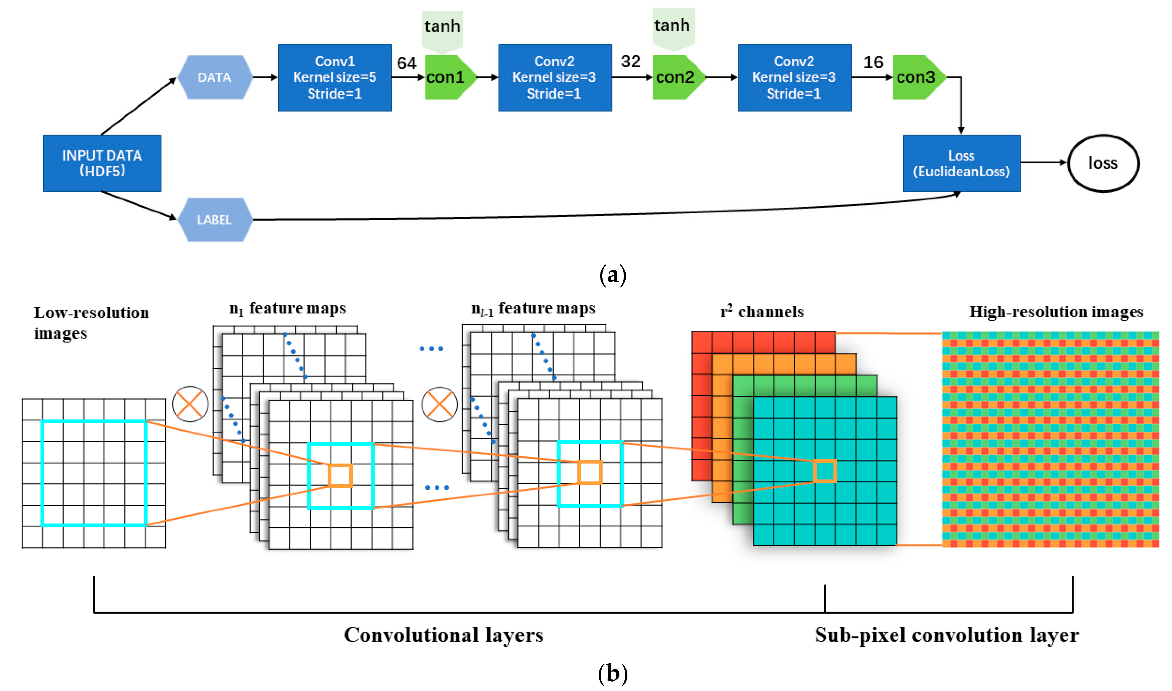
Figure 1 shows the framework and parameters of the ESPCN. ESPCN first applies the 3-layer convolutional neural network directly to low-resolution images to avoid experiencing an amplification before entering the network. After three convolution operations, the low-resolution image is mapped into a feature map with channels, and r is the upscaling factor. Finally, the high-resolution image is generated by a sub-pixel convolution layer. The sub-pixel convolutional layer enhances its memory for a position by periodically filtering functions, combining feature maps with channel into high-resolution images.
The basic calculation of the network is shown in Equations (1)–(4). Equation (1) and Equation (2) follow the principle of convolution theory.
is the low-resolution image of the input network, is the high-resolution image learned by ESPCN, and is the convolution kernel function ( is the convolution layer). and are the weight and bias parameters of the convolution kernel, which are obtained by iterative learning of the network. is a nonlinear activation function. Equations (3) and (4) are function descriptions of the subpixel convolution part. is a periodic shuffle operator, which can reorder tensors of size to tensors of size .
Feeding the oversize image block to the ESPCN method will greatly affect the network effects; therefore, our paper reconstructed the input low-resolution MODIS image twice with the upsampling factor r = 4. The parameters of the network were set to = 3, () = (5, 64), () = (3, 32), and = 3, = 4. For the training samples of network learning, the image pairs are composed of the original Landsat image and the downsampled image to the 1/4 of the original image pair, and the 1/4 image and the further downsampled 1/4 low-resolution image pair. To avoid repetitive training of the original image pixels, the stride for extracting the sub-image blocks from the original image was , and the stride for extracting the sub-image blocks from the lower resolution image in the image pair was .
2.3. Improved Spatiotemporal Fusion Model SR-FSDAF
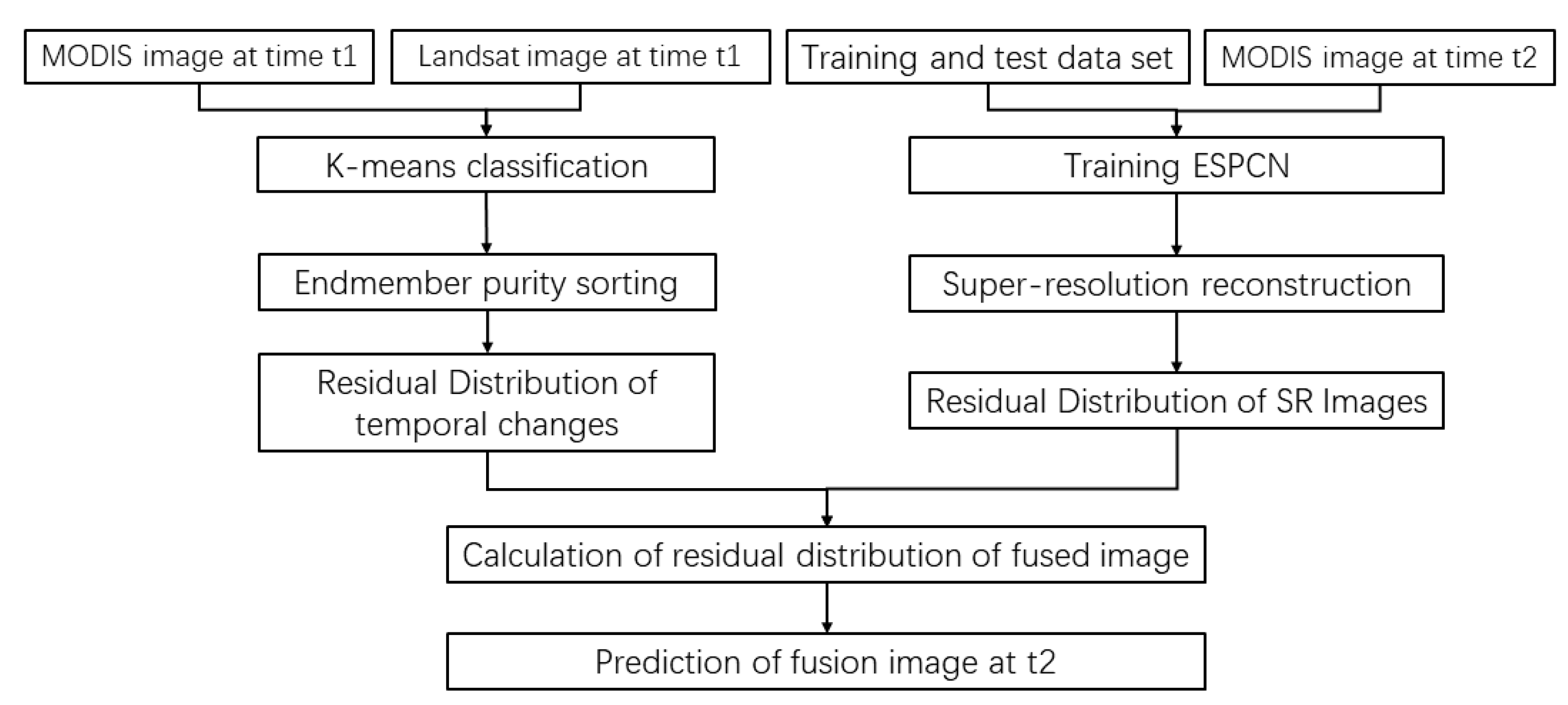
SR-FSDAF combines the super-resolution algorithm and the flexible Spatio-temporal data fusion model algorithm. The SR-FSDAF has six steps: The computing of MODIS pixel purity based on unsupervised classification, coarse estimation of the pixel temporal change, residual computing of pixel temporal changes, image reconstruction and spatial change prediction based on ESPCN super-resolution, residual distribution calculation, and enhancement and fusion based on neighborhood information. For the convenience of the description, the high spatial resolution Landsat image is defined as fine images, and the high temporal resolution MODIS image is expressed as coarse images. Landsat and MODIS images at and the MODIS image at t2 are used to predict Landsat images at t2.
Figure 2 shows the flow of the algorithm. The detailed principle of the algorithm refers to in FSDAF [32] and ESPCN [40]. The variables and definitions of the model are as follows:
—the pixel number of the corresponding Landsat-8 image in a MODIS pixel, which is a constant of 16;
—the coordinates of the ith MODIS pixel;
—MODIS pixel index;
—index of Landsat-8 pixels in a MODIS pixel index (: 1, 2, …, m);
, —Values of band on MODIS pixel at and ;
, —Values of the th Landsat-8 pixel in band at MODIS pixel at and ;
—the proportion of class c Landsat-8 pixels in the th MODIS pixel;
the change of the ith MODIS pixel from to at band ;
—changes of category pixels on the th band of Landsat-8 images from to , and is one of the classification results of ground objects.
2.3.1. Unsupervised Classification of Landsat Images at Time
Through image preprocessing, the spatial resolution of the MODIS image is 480 m. The spatial resolution of the Landsat image is 30 m. Therefore, the coverage area of one MODIS pixel is the same as that of 16 Landsat pixels. Based on this correspondence, we use the K-means algorithm to classify the Landsat images at time t1 and set the number of clustering to four categories: water, farmland, buildings, and woodland. represents the proportion of Landsat pixels of classification c in 16 pixels (c = 1, … 4). For calculation, see Formula (5). is the number of Landsat pixels of classification c in 16 pixels.
The K-means method first calculates the initial mean of the categories uniformly distributed in the data space and then iterates with the principle of the shortest distance to aggregate the pixels into the nearest cluster. Recalculate the mean values of classes in each iteration and reclassify pixels with these mean values until the variance within classes meets the requirements.
2.3.2. Rough Estimation of Pixel Temporal Change
The second step is calculating the change of MODIS image reflectivity from to . The calculation formula shows in Equation (6).
According to the spectral unmixing principle, the spectral value of the MODIS pixel can be expressed by the weighted calculation results of the spectral reflectance value of various ground objects in the pixel. Therefore, the temporal variation of the MODIS pixel can also be calculated by the Formula (7). The in the Formula (7) is variation values of Landsat class objects on band , which can be obtained by least squares inverse solution the Formula (7).
Sort the values of c-class ground objects in MODIS pixels from large to small. The larger the -value is, the higher the proportion of c-type ground objects in MODIS pixels is, and the purer the pixels are. According to the values, select n MODIS pixels from high to low to solve .
2.3.3. Residual Computing of Pixel Temporal Changes
Assuming that there is no spectral information mutation in the ground object, the prediction result of the fine-resolution image at time is . The calculation of the prediction result shows in Formula (8):
Usually, the spectral information of the ground objects will change between the two moments, and the resulting deviation defines as . The calculation Formula shows in Formula (9), where n is 16.
2.3.4. Image Reconstruction and Spatial Change Prediction Based on ESPCN Super-Resolution
Using the ESPCN network, MODIS images at time are input to obtain higher resolution images reconstructed by the super-resolution algorithm. The residual between the high-resolution image obtained by the ESPCN method and the true high-resolution image at can express as :
The ESPCN method directly applies the convolution layer to the coarse image to avoid the loss of detailed information. The sub-pixel convolution layer restores the feature map to the super-resolution image. The input MODIS images obtain a high-resolution image by three consecutive convolution operations and sub-pixel layer rearrangement. ESPCN learns the feature mapping relationship between coarse and fine images more comprehensively and can retain the spatial feature information of the input image.
2.3.5. Residual Distribution Calculation
This step uses the homogeneity index to assign weights to residual and residual to calculate the final residual. The difference between the two prediction results calculates as the difference residual , which shows as Formula (11):
Use the 4 × 4 moving window to calculate the ratio of the number of pixels consistent with the ground object category of the central fine-resolution pixel to the total number of pixels in the window as the homogeneity index. The calculation Formula is (12), where is the central pixel of the moving window. When the pixel categories in the window are consistent, the value of is 1, otherwise is 0.
Calculate the weight according to the homogeneity index (Formula (13)). The change degree of homogeneous pixels is determined based on the prediction of ESPCN super-resolution, and the change degree of heterogeneous pixels is determined based on the prediction of ESPCN super-resolution.
Normalize the to obtain (Formula(14)):
Calculate the residual distribution of the predicted fine resolution image based on the normalized weight (Formula (15)). Then, calculate the change value of fine-resolution pixel from time to time , as shown in Formula (16).
2.3.6. Enhancement and Fusion Based on Neighborhood Information
Use the neighborhood information to improve the prediction stability and reduce the block effect caused by calculation. For the fine-resolution image pixel at time , n fine pixels with the same class and the least spectral difference with the in the neighborhood are selected. The computation formula of spectral difference between the kth fine-resolution pixel and the similar neighborhood pixel is , as shown in Formula (17).
The weight contribution of these similar pixels to the center pixel follows the distance principle (Formula (18)). The size of w in depends on the size of the neighborhood when taking 20 similar pixels. The farther the distance, the smaller the weight contribution value. After normalization, the calculation formula of weight is (19):
After adding the neighborhood information, the final prediction image result is (20):
2.4. Inversion Models
In the process of remote sensing quantitative inversion, the accurate selection of characteristic bands is the basis for obtaining high inversion accuracy. We use the concentration the value of water quality parameter NH3-N to calculate the correlation coefficient between reflectivity and band combinations and select the band or band combination with high correlation as the modeling parameter.
The traditional statistical regression model (TSR) has been widely used in the inversion of water quality parameters [41,42].In this paper, the linear function, quadratic function, exponential function, and logarithmic function are used to construct the inversion model (Table 1). The model with the highest inversion accuracy is selected as the model type of the traditional statistical regression model.
At the same time, this paper selects the random forest model with high learning efficiency as the machine learning algorithm to train and obtains the machine learning model for the back study of water quality parameters.
2.5. Evaluation Index
To evaluate the accuracy of the fusion method, this paper uses three algorithms: STARFM, FSDAF, and SRCNN embedding FSDAF as comparison methods. We analyze the experimental results from the qualitative evaluation and quantitative evaluation. The qualitative evaluation method compares the fusion results of different models at time with Landsat images at time . Through visual observation, we can determine whether the local details and the overall spectral difference are too large in the simulation reality. The quantitative evaluation method uses three evaluation indexes to comprehensively evaluate the overall structural similarity of the fused image, the degree of reflectivity reduction of the fusion image, and the spectral fidelity of the fusion image.
The overall structural similarity index is structural similarity SSIM, which is widely used to evaluate the linear relationship strength of two similar images. The calculation method shows in Formula (21):
and are the average values of the Landsat image and the fused image at time t2, respectively; and are the image variances of the two; and are non-0 constants used to ensure that the results are rational. The more similar the overall structure of the two images is, the closer the SSIM value is to 1.
The evaluation index of reflectivity reduction degree is the root mean square error RMSE, which reflects the simulation fusion results of pixel value reduction degree and detail information. The formula shows in (22). is the Landsat true image, and is the fusion image.
The evaluation index used for spectral fidelity is the spectral angle SAM (Spectral angle Mapper), which regards the single-pixel spectrum as a high-dimensional vector and calculates the vector angle of the spectral vector of the pixels in the same position of the two images. The smaller the value is, the more similar the spectrum between the pixels is. The specific angle calculation formula is as follows (23).
The accuracy of the inversion model was evaluated by a fitting coefficient (R2), mean absolute percentage error (MAPE), and root mean square error (RMSE). The formula of MAPE shows in (24).
2.6. Study Area
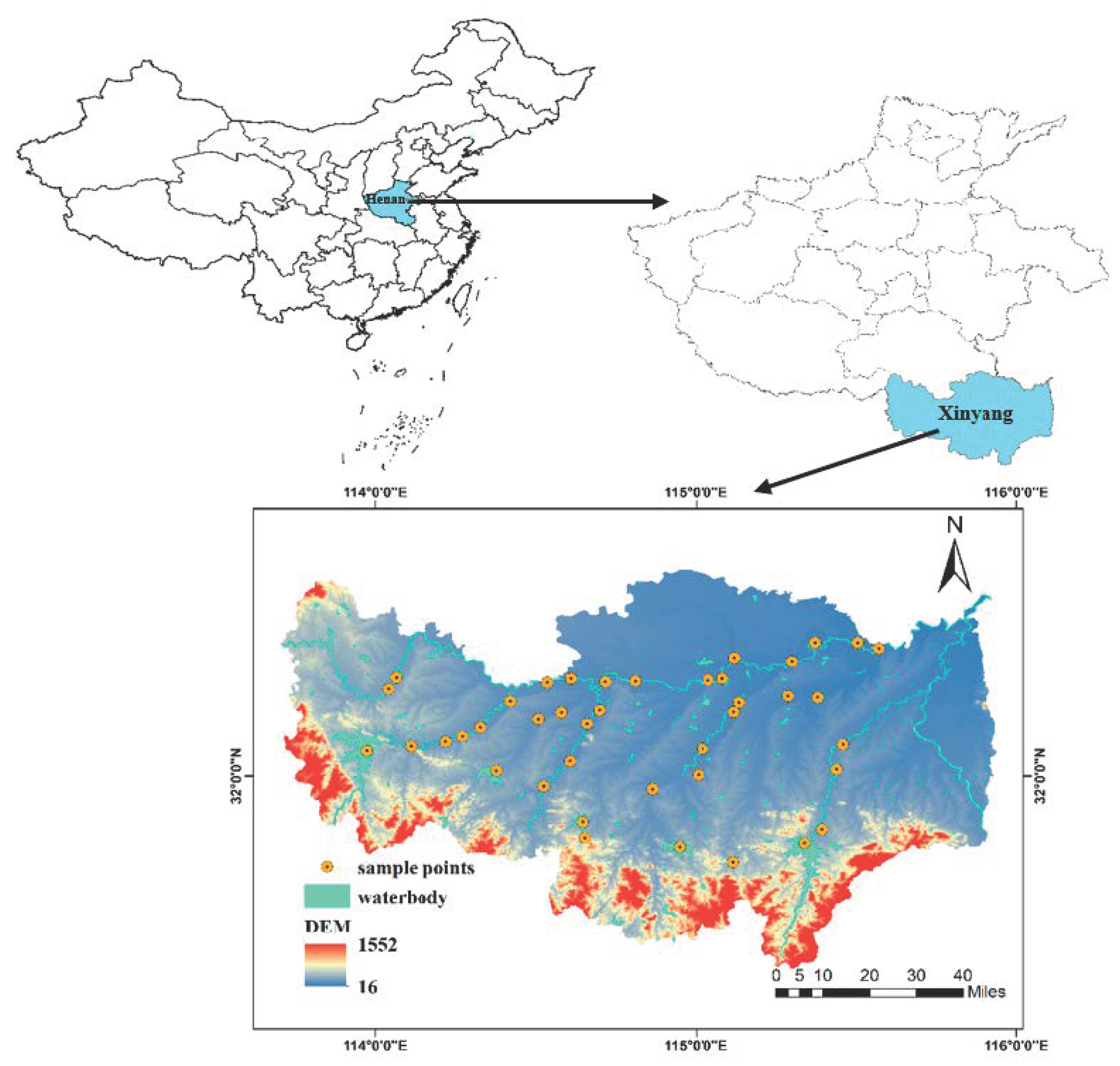
The study area is 113°45′ E~115°55′ E, 30°23′ N~32°27′ N in the Xinyang section of Huaihe River Basin. The study area is located on the boundary line between North and South China (Qinling–Huaihe Line), which belongs to the transition zone between subtropical and temperate monsoon climates and the transition zone between humid and semi-humid regions. The main tributaries in the region are shown in Figure 2.
On 5 December 2016 and 1 January 2017, the concentrations of NH3-N in 43 water samples were collected in the study area. The distribution of the measured sampling points and the location of the study area are shown in Figure 3.
2.7. Landsat-8 OLI
The spatial resolution of Landsat-8 is 30 m, and the return visit period is 16 days, which is the fusion data source commonly used in the Spatio-temporal fusion algorithm. For the test of the fusion model, two sets of MODIS-Landsat image pairs are used in this paper.
The first group is the Landsat and MODIS image pairs of Xinyang City on 8 November 2017, and 24 November 2017. No heterogeneous mutation occurred during the period. The second group is the Landsat and MODIS image pairs on 26 November 2004, and 12 December 2004, in northern New South Wales, Australia, during which flood events in the region caused heterogeneous mutations.
NH3-N inversion of remote sensing data selected less than 10% of the cloud Landsat-8 OLI data, image bands, and other specific information can be seen in the Table 2. The selected Landsat-8 OLI images were preprocessed, such as atmospheric correction.
2.8. MODIS
MODIS has a spatial resolution of 500 m and a return visit period of 1 day, a commonly used fusion data source for Spatio-temporal fusion algorithms.
For the fusion model and NH3-N inversion experiments, this paper uses MODIS daily surface reflectance data on the same date as the corresponding Landsat. The selected MODIS data has been preprocessed, and the MODIS is reprojected and resampled to 480 m to facilitate matching and calculation with Landsat image pixels with a spatial resolution of 16 m. The specific information of MODIS is shown in the Table 3.
3. Experiments and Results
3.1. Evaluations of Spatio-Temporal Fusion Model
Cut the Landsat and MODIS images to specified size so that the ratio of the Landsat and MODIS image is 16:1. From Table 2 and Table 3, the band ranges of B2, B3, B4, B5, B6, and B7 of Landsat-8 were similar to those of B3, B4, B1, B2, B6, and B7 of MODIS, respectively.
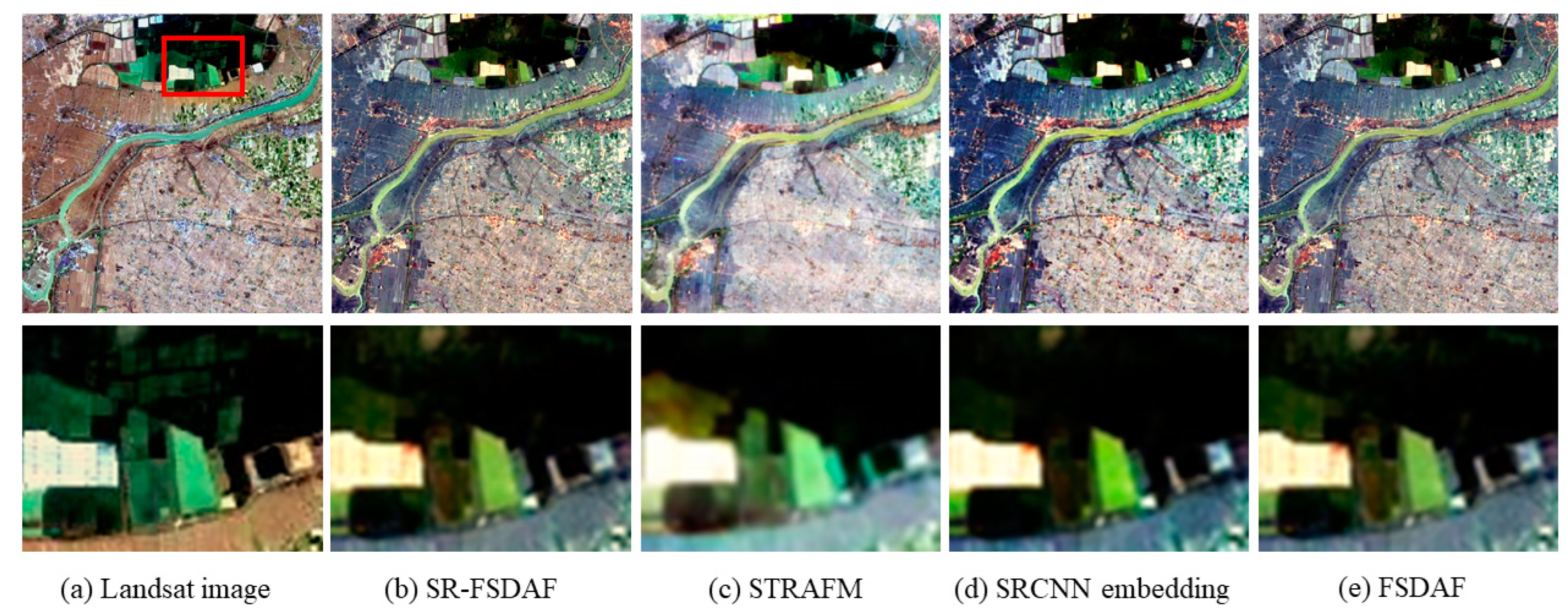
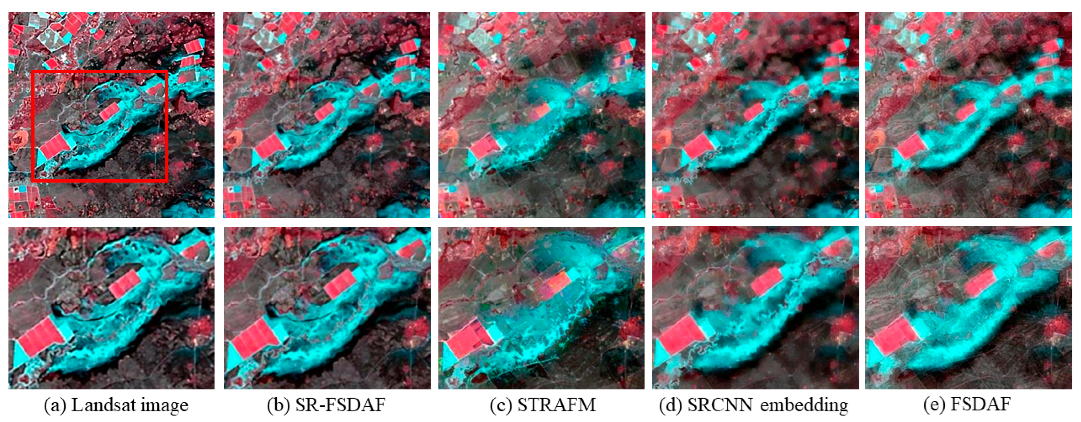
Twelve bands of Landsat-8 (B2, B3, B4, B5, B6, and B7) and MODIS (B3, B4, B1, B2, B6, and B7) were put into the SR-FSDAF model to obtain the fusion image of the predicted date. The fusion results of the first kind of non-heterogeneous mutation are shown in Figure 4. From the perspective of subjective vision, the SR-FSDAF can capture and retain details of the local better.
From the fusion result images, STARFM, SRCNN-embedded model, FSDAF, and SR-FSDAF have obtained similar fusion results with the true Landsat image. The SRCNN-embedded method is similar to the SR-FSDAF, and SRCNN is used instead of TPS for upsampling. Through the partial detail comparison, SR-FSDAF retains more details of the roof.
Table 4 shows the specific calculated values of RMSE, SSIM, and SAM of the four methods in Figure 4. The best fusion result values of each band are highlighted by thick lines. The optimal value of SAM is 3.417 of SR-FSDAF, indicating that the fused image of SR-FSDAF has the maximum relative spectral fidelity.
Table 4 shows the specific calculated values of RMSE, SSIM, and SAM of the four methods in Figure 5. The best fusion result values of each band are highlighted by thick lines. The optimal value of SAM is 3.417 of SR-FSDAF, indicating that the fused image of SR-FSDAF has the maximum relative spectral fidelity.
On Band1, FSDAF achieved better fusion results. For Band 2–Band 7, SR-FSDAF obtained better values in RMSE and SSIM. The performance of SR-FSDAF proposed in this paper on SSIM and RMSE is equivalent to that of FSDAF and SRCNN embedding models on some bands, but the total results of SR-FSDAF are the best, and it has an excellent performance in structure similarity and detail retention. The performance of FSDAF and SRCNN embedded models is the second, and the results of STARFM are the worst.
The ground objects of the second group of experimental images changed abruptly in the period. From the fusion result (Figure 5), STARFM, SRCNN embedding model, FSDAF, and SR-FSDAF obtained similar fusion results. The SR-FSDAF method is more accurate in capturing the change of ground objects and detailed information, but the fusion results of all mutation methods are less satisfactory than those of the first group.
Table 5 shows specific values of the three evaluation indexes of the four methods of the second set of images. The best fusion results for each band are sharpened and underlined. The optimal value of SAM is 7.439 of SR-FSDAF. Band1–Band7 index optimal value method is SR-FSDAF, FSDAF and SR-FADAF index performance is similar. SR—FADAF still has the best fusion result among the four methods when the ground changes. However, compared with the fusion results of the regions without mutation in the first group, the fusion quality of the four methods decreases on heterogeneous changes.
3.2. Inversion Based on Fused Images
3.2.1. Correlation Analysis of NH3-N
The measured data of water samples collected from 43 sampling points of Xinyang key water function areas on 5 December 2016 and 1 January 2017 are randomly selected for 70%. We analyzed the Pearson correlation coefficient between 70% of the measured data and the different bands or band combinations of the fused images generated by Landsat and MODIS images on 7 December 2016, and 30 December 2016.
The correlations among the bands and their simple combinations were calculated. Taking two different bands of A and B as examples, the correlation of A, B, (A + B), (A − B), (A/B), (A − B)/(A + B) is calculated, respectively, and the highest correlation coefficient among these combinations was taken as the R value between A and B to draw the correlation matrix.
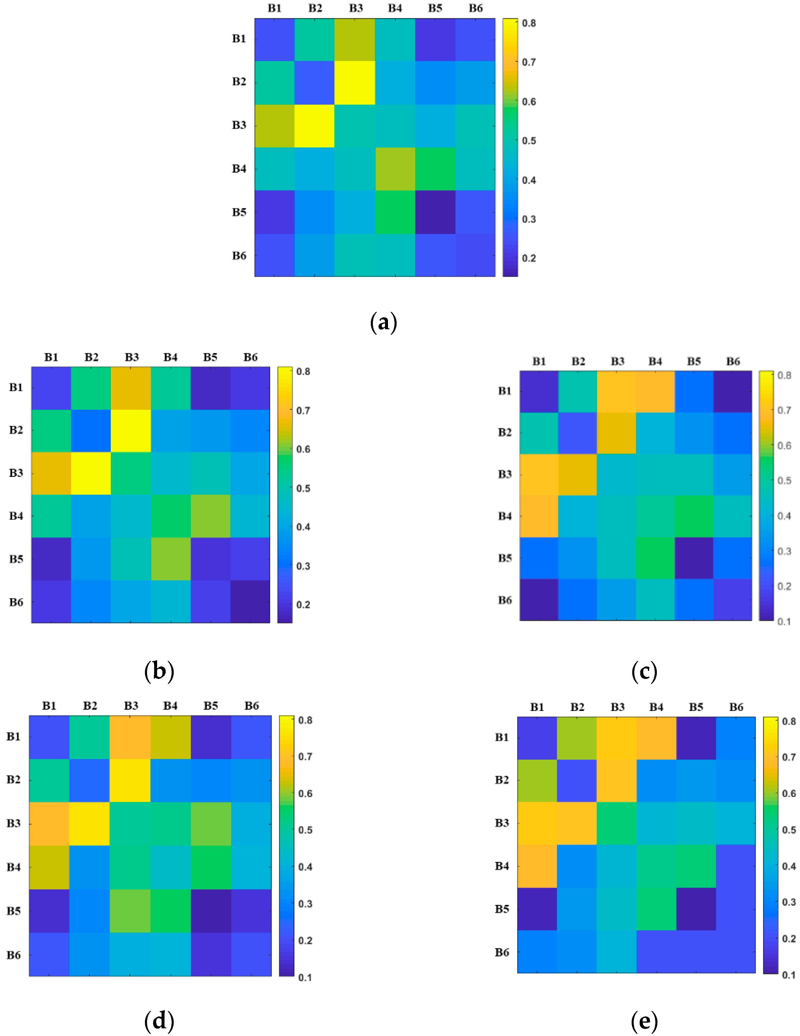
We calculated the correlation between NH3-N and these band combinations of different fusion images and Landsat-8 images. The results were drawn into a correlation matrix (Figure 6).
Selected bands or band combinations with correlations above 0.7 (Table 6). We found that the highest NH3-N correlation band of STARFM changed to B/R after spatiotemporal fusion. The highest correlation bands of SR-FSDAF, SRCNN embedding model, and FSDAF are consistent with Landsat images, which are (R − G)/(R + G). The correlation between SR-FSDAF and Landsat-8 was consistent, 0.81. This means that the surface reflection in the SR-FSDAF fusion image is highly similar to that in the original image. The SR-FSDAF fusion image can be used for the inversion of water quality parameters.
3.2.2. Accuracy Comparison of Inversion Models
We constructed inversion models of NH3-N based on statistical regression and random forest using the SR-FSDAF fusion image, respectively. In this paper, we used 64 samples to train the model and the remaining 24 samples for accuracy verification. The accuracy of the models was evaluated by the difference between the measured and estimated values.
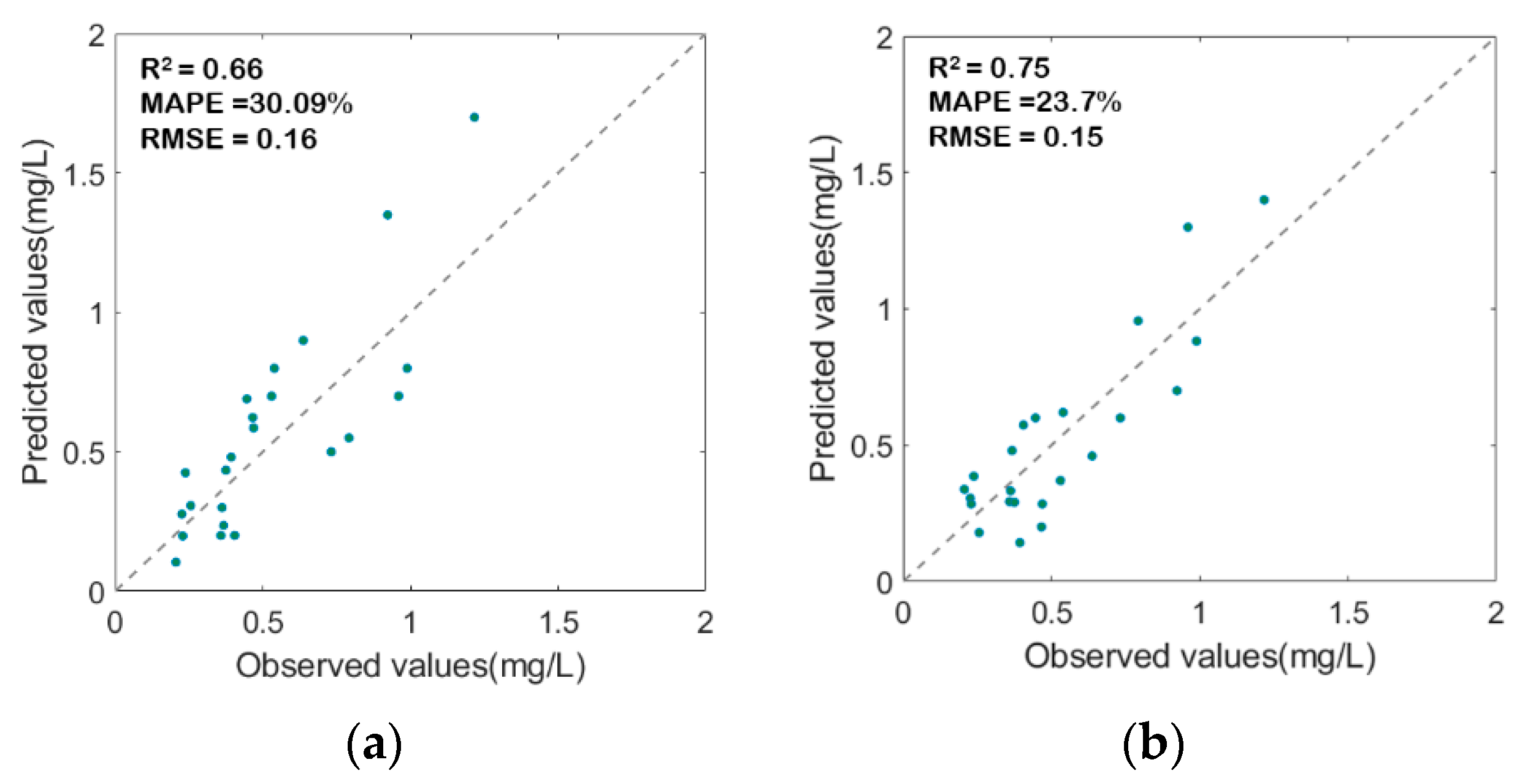
The optimal model inversion results are shown in Figure 7 with the band combination of Red and Green. The optimal results of the statistical regression method are shown in Figure 7a. The R2 is 0.66, RMSE is 0.16, and MAPE is 30.1%. The optimal inversion results based on the random forest method are shown in Figure 7b for the combination of Blue, Green, Red, and NIR. The R2 was 0.75, RMSE was 0.15, and MAPE was 23.7%. The results showed that the random forest method had great advantages in estimating NH3-N concentration.
3.2.3. Spatio-Temporal Distribution of the NH3-N
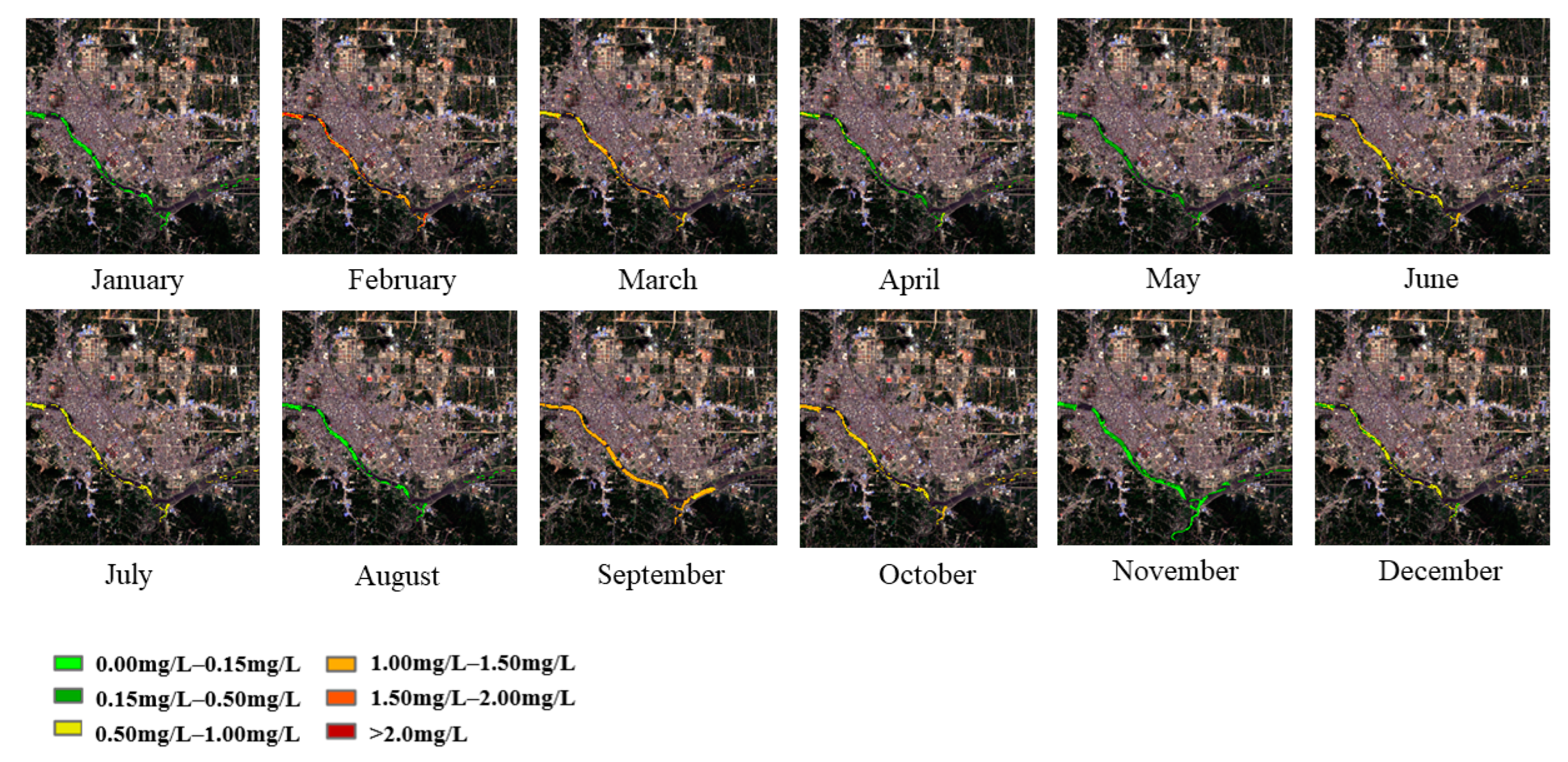
This paper conducted further research based on the random forest inversion model. The inversion diagrams of NH3-N concentration from January to December 2017 were obtained by inversion, and its distribution characteristics and variation trend were analyzed.
Figure 8 shows the percentage of water surface area of different NH3-N concentration levels in twelve months. According to the relevant survey data, the Huaihe River system is a wet season from July to August, a dry season from December to February, and a water-stable season in other months. The changes in NH3-N concentrations in different periods and the classification standard for NH3-N concentration are shown in Table 7. Figure 9 shows our classification of NH3-N concentrations and the distribution of NH3-N in January 2017.
Comprehensive Figure 8 and Table 7, the main component of the water body in the wet season is type II NH3-N concentration water; the water quality is the best, the NH3-N concentration is the lowest, and the changing trend is gentle.
NH3-N concentration of water body in stable period is greatly disturbed. The NH3-N concentration is relatively high in the early water stability period from March to June, and the NH3-N concentration is relatively low in the late water stability period from September to November.
The concentration of NH3-N is the highest in the dry season and changes gently. In the dry season, the lowest concentration of NH3-N is in December, mainly Class II and III concentrations. From December to February, the concentration of NH3-N gradually increased. The area ratio of type InferiorV NH3-N concentrated water increased and concentrated in the central region in January.
4. Discussion
The reflectance characteristics of different concentrations of water quality parameters in a specific wavelength range are the analytical basis for the quantitative inversion of water quality parameters using the spectral information of remote sensing images. Our study shows that the sensitive bands of NH3-N are Blue, Green, Red, and NIR, showing the combined frequency characteristics of nitrogen-containing functional groups.
In the actual research process, remote sensing inversion is completed by establishing effective connections between the point data obtained by field sampling and the surface data of remote sensing pixels with different spatial resolutions. The difference between the sampling and the satellite transit time, the limited water quantity of inland water, and the significant Spatio-temporal changes cause the error of inversion results. Use the Spatio-temporal fusion method to reduce the bias and reflect the change in water quality parameters better, which is the significance of this study. The time resolution of Landsat images is increased by using the Spatio-temporal algorithm and generating a series of high-frequency sequential images for water quality inversion.
The SR-FSDAF model has better visual effects and index results than the STARFM, SRCNN embedding model, and FSDAF in the case of non-heterogeneous mutation and heterogeneous mutation. For non-heterogeneous mutation images, RMSE, SSIM, and SAM of SR-FSDAF are 0.03 (mean), 0.976 (mean), and 3.417, respectively, and for heterogeneous mutation regions, RMSE, SSIM, and SAM are 0.021 (mean), 0.810 (mean) and 7.439, respectively.
To prove the advantages of the SR-FSDAF fusion method for water quality monitoring, STARFM, SRCNN embedding model, FSDAF, and SR-FSDAF fusion image are used to calculate the correlation coefficient distribution of different band combinations and NH3-N. The most sensitive band combination and correlation of SR-FSDAF are highly consistent with Landsat-8 images. Therefore, the SR-FSDAF method can be used for quantitative inversion of water quality parameters.
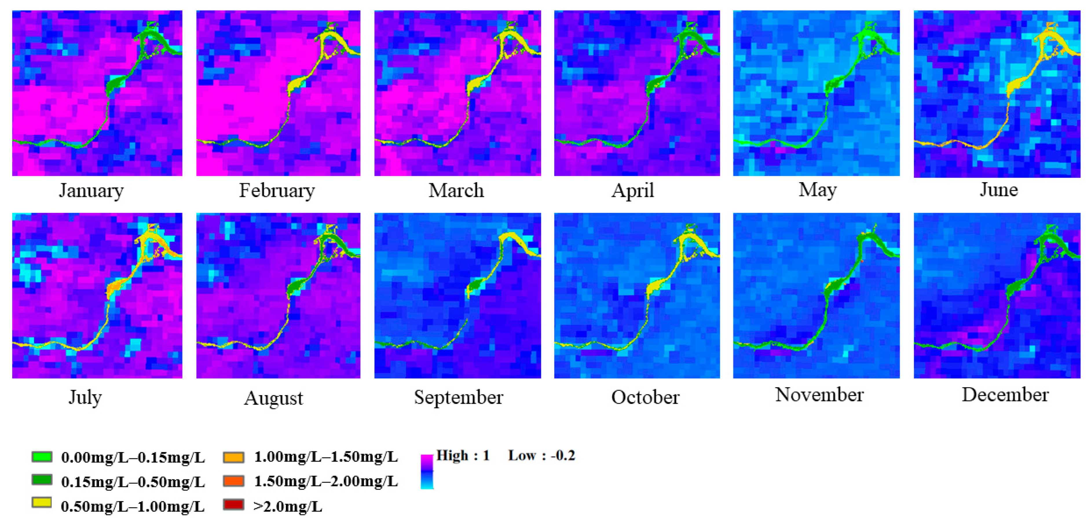
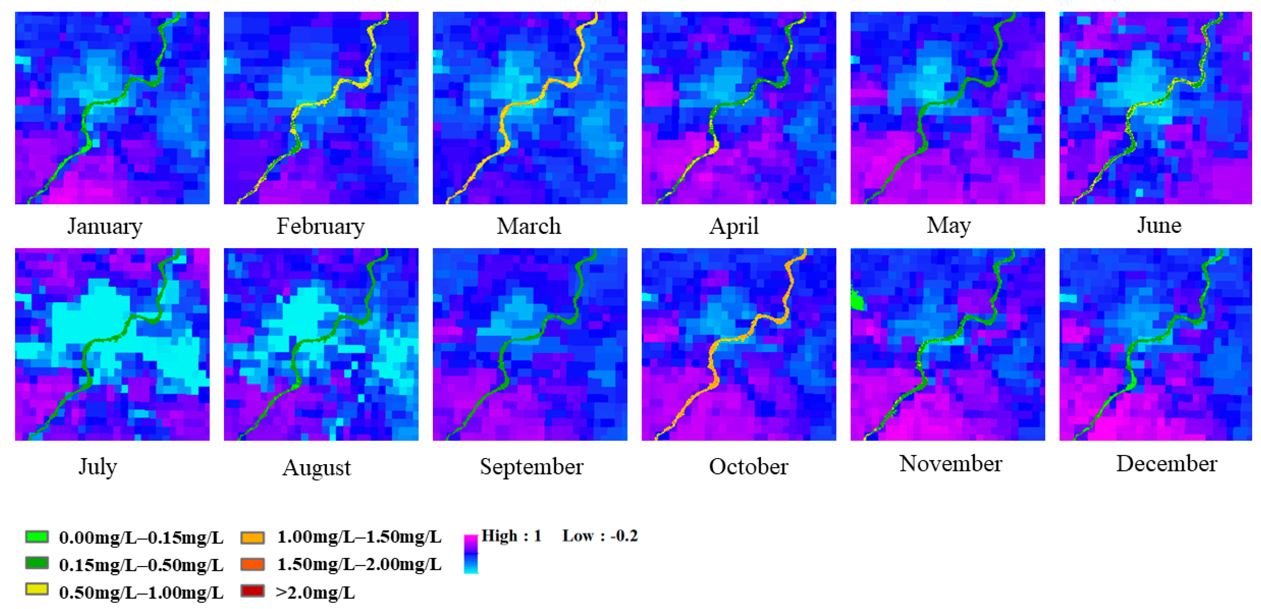
The change in water quality is closely related to the evolution of the surrounding environment. NH3-N is an essential fertilizer for crop growth and a common component in industrial and domestic sewage. The concentration of NH3-N in water is often affected by sewage discharge from human production and life and drugs and fertilizers used in agricultural activities. To further analyze the temporal and spatial variation characteristics of water quality in Xinyang City, we selected four regions (Figure 9a–d). According to the 1 km-land use classification map of Xinyang City in 2017 (Figure 10) and field survey, region (a) is the main industrial region. (b) and (c) are farmland on both sides of the river, mainly dry and paddy fields. The river in (d) passes through residential areas.
Figure 11, Figure 12, Figure 13 and Figure 14 show the monthly NH3-N concentration changes in the four regions. Figure 12, Figure 13 and Figure 14 contain more farmland, so we compare the NH3-N concentration and NDVI results to verify its relationship with agricultural activities. According to the subtropical and temperate monsoon climate in the same period of rain and heat in Xinyang City, if there is no interference from human activities, the change of NH3-N concentration is mainly affected by the amount of river water, which is higher in December to February and lower in June to August.
In Figure 11, the river mainly flows through industrial production areas, where NH3-N concentrations are highest in February, March, September, and October. NH3-N concentration was low in January, May, August, and November. The NH3-N concentration in this area did not show obvious seasonal variation and was mainly affected by industrial wastewater discharge.
Figure 12 is mainly farmland area. According to the land use data, the area is mainly dry land, and the main crop is wheat. It can be seen that during the growth period of wheat from January to April and the maturity period of wheat in July, the concentration of NH3-H is higher due to the use of fertilizer.
The area in Figure 13 is mainly a paddy field, planting crops for rice. During the rice growing season from February to July, the NH3-N concentration in the river was higher.
Figure 14 shows the mixed area of residential land and farmland. The annual variation of NH3-N concentration in this area is relatively gentle, and there is no obvious seasonal variation or agricultural production law, which belongs to the area affected by many factors.
Figure 12 and Figure 13 show the partial interception of Huaihe River, which is the largest river in the Xinyang area with a large water volume and fast flow velocity. Due to the uneven distribution of water quality and the difference in flow velocity, the difference in NH3-N concentration at the edge and center of the river is obvious.
Overall, during the rainy season, the NH3-N concentration was diluted by rainwater, and the overall concentration was lower than in other periods; the concentration of NH3-N was the highest in the dry season, and the concentration changed gently. In addition to the impact of human activities, during the agricultural production period from January to August, pollution, such as chemical fertilizers in farmland, will lead to the increase in NH3-N concentration in water, which corresponds to the research results of other scholars [20]. The irregular high concentration of NH3-N in cities is mainly caused by industrial wastewater discharge.
5. Conclusions
In this study, an improved SR-FSDAF Spatio-temporal fusion model was proposed and applied to monitor NH3-N concentration in small and medium inland waters (Xinyang section of Huaihe River Basin). We studied the relationship between the field NH3-N data and the fused image band. The research shows that SR-FSDAF provides an effective monitoring method to improve the monitoring frequency and maintain the accuracy of water quality prediction and has great application potential in quantitative remote sensing of water quality. The random forest model constructed in this paper can be used as a high-precision and efficient method for water quality prediction in the Xinyang section of the Huaihe River Basin and provide data support for water quality monitoring and water pollution control in the Huaihe River Basin.
Although the SR-FSDAF model achieves a better fusion effect, its prediction accuracy for heterogeneous mutation is still not ideal, mainly because the spectral details of MODIS images are very limited. At the same time, whether the SR-FSDAF model has achieved similarly good results in the fusion of satellite images from other data sources remains to be demonstrated. In future work, we will test the performance of the model in the Spatio-temporal fusion of different images. In addition, more spectral information is obtained from multiple dimensions by using learning methods to improve the prediction of heterogeneous mutations. For NH3-N remote sensing monitoring, more work is needed to prove the adaptability of the random forest model to different regions.
Author Contributions
Conceptualization, M.K. and J.L.; methodology, M.K. and J.L.; software, M.K.; validation, M.K.; formal analysis, M.K. and Y.M.; investigation, M.K. and J.C.; resources, J.L.; data curation, M.K. and J.C.; writing—original draft preparation, M.K.; writing—review and editing, M.K. and J.L.; visualization, M.K.; supervision, J.L.; project administration, J.L. All authors have read and agreed to the published version of the manuscript.
Funding
This study was supported by National Natural Science Foundation of China (Key Program) (Grant No. 51739009) and 2019 Henan Province Natural Science and Technology Project (Henan Natural Letter [2019] No. 373-11).
Data Availability Statement
Landsat OLI and MODIS images: https://www.usgs.gov/products/data/all-data; NDVI products: National Earth System Science Data Center, National Science & Technology Infrastructure of China (http://www.geodata.cn).
Acknowledgments
Acknowledgement for the NDVI data support from “National Earth System Science Data Center, National Science & Technology Infrastructure of China (http://www.geodata.cn)”.
Conflicts of Interest
The authors declare no conflict of interest.
References
- Zinabu, E.; Kelderman, P.; van der Kwast, J.; Irvine, K. Evaluating the Effect of Diffuse and Point Source Nutrient Transfers on Water Quality in the Kombolcha River Basin, an Industrializing Ethiopian Catchment. Land Degrad. Dev. 2018, 29, 3366–3378. [Google Scholar] [CrossRef] [Green Version]
- Gong, S.Q.; Huang, J.Z.; Li, Y.M.; Lu, W.N.; Wang, G.X. Preliminary Exploring of Hyperspectral Remote Sensing Experiment for Nitrogen and Phosphorus in Water. Spectrosc. Spectr. Anal. 2008, 28, 839–842. [Google Scholar]
- Wang, X.; Fu, L.; He, C. Applying Support Vector Regression to Water Quality Modelling by Remote Sensing Data. Int. J. Remote Sens. 2011, 32, 8615–8627. [Google Scholar] [CrossRef]
- Liu, H.; Xuejian, L.; Fangjie, M.; Meng, Z.; Di’en, Z.; Shaobai, H.; Zihao, H.; Huaqiang, D. Spatiotemporal Evolution of Fractional Vegetation Cover and Its Response to Climate Change Based on Modis Data in the Subtropical Region of China. Remote Sens. 2021, 13, 913. [Google Scholar] [CrossRef]
- Kun, S.; Zhang, Y.; Zhu, G.; Qin, B.; Pan, D. Deteriorating Water Clarity in Shallow Waters: Evidence from Long Term Modis and in-Situ Observations. Int. J. Appl. Earth Obs. Geoinf. 2017, 68, 287–297. [Google Scholar]
- Zhang, Y.; Shi, K.; Zhou, Y.; Liu, X.; Qin, B. Monitoring the River Plume Induced by Heavy Rainfall Events in Large, Shallow, Lake Taihu Using Modis 250m Imagery. Remote Sens. Environ. 2016, 173, 109–121. [Google Scholar] [CrossRef]
- Gebru, H.G.; Melesse, A.M.; Gebremariam, A.G. Double-Stage Linear Spectral Unmixing Analysis for Improving Accuracy of Sediment Concentration Estimation from Modis Data: The Case of Tekeze River, Ethiopia. Model. Earth Syst. Environ. 2020, 6, 407–416. [Google Scholar] [CrossRef]
- Heng, L.; Wang, Y.; Jin, Q.; Shi, L.; Li, Y.; Wang, Q. Developing a Semi-Analytical Algorithm to Estimate Particulate Organic Carbon (Poc) Levels in Inland Eutrophic Turbid Water Based on Meris Images: A Case Study of Lake Taihu. Int. J. Appl. Earth Obs. Geoinf. 2016, 62, 69–77. [Google Scholar]
- Arias-Rodriguez, L.F.; Zheng, D.; Sepúlveda, R.; Martinez-Martinez, S.I.; Disse, M. Monitoring Water Quality of Valle De Bravo Reservoir, Mexico, Using Entire Lifespan of Meris Data and Machine Learning Approaches. Remote Sens. 2020, 12, 1586. [Google Scholar] [CrossRef]
- Md, M.; Jannatul, F.; KwangGuk, A. Empirical Estimation of Nutrient, Organic Matter and Algal Chlorophyll in a Drinking Water Reservoir Using Landsat 5 Tm Data. Remote Sens. 2021, 13, 2256. [Google Scholar]
- Montanher, O.C.; Novo, E.M.L.M.; Barbosa, C.C.F.; Rennó, C.D.; Silva, T.S.F. Empirical Models for Estimating the Suspended Sediment Concentration in Amazonian White Water Rivers Using Landsat 5/Tm. Int. J. Appl. Earth Obs. Geoinf. 2014, 29, 67–77. [Google Scholar] [CrossRef]
- Shi, L.; Mao, Z.; Wang, Z. Retrieval of Total Suspended Matter Concentrations from High Resolution Worldview-2 Imagery: A Case Study of Inland Rivers. IOP Conf. Ser. Earth Environ. Sci. 2018, 121, 032036. [Google Scholar] [CrossRef]
- Martin, J.; Eugenio, F.; Marcello, J.; Medina, A. Automatic Sun Glint Removal of Multispectral High-Resolution Worldview-2 Imagery for Retrieving Coastal Shallow Water Parameters. Remote Sens. 2016, 8, 37. [Google Scholar] [CrossRef] [Green Version]
- Liu, H.; Zheng, L.; Jiang, L.; Liao, M. Forty-Year Water Body Changes in Poyang Lake and the Ecological Impacts Based on Landsat and Hj-1 a/B Observations. J. Hydrol. 2020, 589. prepublish. [Google Scholar] [CrossRef]
- Nazeer, M.; Nichol, J.E. Combining Landsat Tm/Etm+ and Hj-1 a/B Ccd Sensors for Monitoring Coastal Water Quality in Hong Kong. IEEE Geosci. Remote Sens. Lett. 2015, 12, 1898–1902. [Google Scholar] [CrossRef]
- Yang, N.; Li, J.D.; Mo, W.; Luo, W.D.; Wu, D.D.; Gao, W.E.; Sun, C.A. Water Depth Retrieval Models of East Dongting Lake, China, Using Gf-1 Multi-Spectral Remote Sensing Images Sciencedirect. Glob. Ecol. Conserv. 2020, 22, e01004. [Google Scholar]
- Du, Y.; Zhang, X.; Mao, Z.; Chen, J. Performances of Conventional Fusion Methods Evaluated for Inland Water Body Observation Using Gf-1 Image. Acta Oceanol. Sin. 2019, 38, 172–179. [Google Scholar] [CrossRef]
- Hickmat, H.; Elham, M.W.; Abdelazim, N.; Takashi, N. Assessing Water Quality Parameters in Burullus Lake Using Sentinel-2 Satellite Images. Water Resour. 2022, 49, 321–331. [Google Scholar]
- Rahul, T.S.; Wessley, B.J.; John, G.J. Evaluation of Surface Water Quality of Ukkadam Lake in Coimbatore Using Uav and Sentinel-2 Multispectral Data. Int. J. Environ. Sci. Technol. 2022; prepublish. [Google Scholar]
- Ustaoğlu, F.; Tepe, Y. Water Quality and Sediment Contamination Assessment of Pazarsuyu Stream, Turkey Using Multivariate Statistical Methods and Pollution Indicators. Int. Soil Water Conserv. Res. 2019, 7, 47–56. [Google Scholar] [CrossRef]
- Zhukov, B.; Oertel, D.; Lanzl, F.; Reinhäckel, G. Unmixing-Based Multisensor Multiresolution Image Fusion. IEEE Trans. Geosci. Remote Sens. 1999, 37, 1212–1226. [Google Scholar] [CrossRef]
- Wu, M.; Niu, Z.; Wang, C.; Wu, C.; Wang, L. Use of Modis and Landsat Time Series Data to Generate High-Resolution Temporal Synthetic Landsat Data Using a Spatial and Temporal Reflectance Fusion Model. J. Appl. Remote Sens. 2012, 6. [Google Scholar]
- Huang, C.; Qin, Z.; Zhang, Z.; Bian, J.; Jin, H.; Li, A.; Zhang, W.; Lei, G. An Enhanced Spatial and Temporal Data Fusion Model for Fusing Landsat and Modis Surface Reflectance to Generate High Temporal Landsat-Like Data. Remote Sens. 2013, 5, 5346–5368. [Google Scholar]
- Gao, F.; Masek, J.; Schwaller, M.; Hall, F. On the Blending of the Landsat and Modis Surface Reflectance: Predicting Daily Landsat Surface Reflectance. IEEE Trans. Geosci. Remote Sens. 2006, 44, 2207–2218. [Google Scholar]
- Hilker, T.; Wulder, M.A.; Coops, N.C.; Linke, J.; Mcdermid, G.; Masek, J.G.; Feng, G.; White, J.C. A New Data Fusion Model for High Spatial- and Temporal-Resolution Mapping of Forest Disturbance Based on Landsat and Modis. Remote Sens. Environ. 2009, 113, 1613–1627. [Google Scholar] [CrossRef]
- Zhu, X.; Chen, J.; Gao, F.; Chen, X.; Mase, J.G. An Enhanced Spatial and Temporal Adaptive Reflectance Fusion Model for Complex Heterogeneous Regions. Remote Sens. Environ. 2010, 114, 2610–2623. [Google Scholar] [CrossRef]
- Li, A.; Bo, Y.; Zhu, Y.; Guo, P.; Bi, J.; He, Y. Blending Multi-Resolution Satellite Sea Surface Temperature (Sst) Products Using Bayesian Maximum Entropy Method. Remote Sens. Environ. 2013, 52–63. [Google Scholar] [CrossRef]
- Liao, L.; Song, J.; Wang, J.; Xiao, Z.; Wang, J. Bayesian Method for Building Frequent Landsat-Like Ndvi Datasets by Integrating Modis and Landsat Ndvi. Remote Sens. 2016, 8, 452. [Google Scholar] [CrossRef] [Green Version]
- Huang, B.; Song, H. Spatiotemporal Reflectance Fusion Via Sparse Representation. IEEE Trans. Geosci. Remote Sens. 2012, 50, 3707–3716. [Google Scholar] [CrossRef]
- Song, H.; Liu, Q.; Wang, G.; Hang, R.; Huang, B. Spatiotemporal Satellite Image Fusion Using Deep Convolutional Neural Networks. IEEE J. Sel. Top. Appl. Earth Obs. Remote Sens. 2018, 11, 821–829. [Google Scholar] [CrossRef]
- Tao, X.; Liang, S.; Wang, D.; He, T.; Huang, C. Improving Satellite Estimates of the Fraction of Absorbed Photosynthetically Active Radiation through Data Integration: Methodology and Validation. IEEE Trans. Geoence Remote Sens. 2017, 56, 2107–2118. [Google Scholar] [CrossRef]
- Zhu, X.; Helmer, E.H.; Feng, G.; Liu, D.; Chen, J.; Lefsky, M.A. A Flexible Spatiotemporal Method for Fusing Satellite Images with Different Resolutions. Remote Sens. Environ. Interdiscip. J. 2016, 172, 165–177. [Google Scholar] [CrossRef]
- Li, X.; Ling, F.; Foody, G.M.; Ge, Y.; Zhang, Y.; Du, Y. Generating a Series of Fine Spatial and Temporal Resolution Land Cover Maps by Fusing Coarse Spatial Resolution Remotely Sensed Images and Fine Spatial Resolution Land Cover Maps. Remote Sens. Environ. 2017, 196, 293–311. [Google Scholar] [CrossRef]
- Xie, D.; Zhang, J.; Zhu, X.; Pan, Y.; Liu, H.; Yuan, Z.; Yun, Y. An Improved Starfm with Help of an Unmixing-Based Method to Generate High Spatial and Temporal Resolution Remote Sensing Data in Complex Heterogeneous Regions. Sensors 2016, 16, 207. [Google Scholar] [CrossRef] [PubMed] [Green Version]
- Zhu, X.; Cai, F.; Tian, J.; Williams, T. Spatiotemporal Fusion of Multisource Remote Sensing Data: Literature Survey, Taxonomy, Principles, Applications, and Future Directions. Remote Sens. 2018, 10, 527. [Google Scholar] [CrossRef] [Green Version]
- Liu, X.; Deng, C.; Wang, S.; Huang, G.; Zhao, B.J. Fast and Accurate Spatiotemporal Fusion Based Upon Extreme Learning Machine. IEEE Geosci. Remote Sens. Lett. 2016, 13, 4. [Google Scholar] [CrossRef]
- Jungho, Y.; Seonyoung, P.; Huili, G. Downscaling of Modis One Kilometer Evapotranspiration Using Landsat-8 Data and Machine Learning Approaches. Remote Sens. 2016, 8, 215. [Google Scholar]
- Moosavi, V.; Talebi, A.; Mokhtari, M.H.; Shamsi, S.; Niazi, Y. A Wavelet-Artificial Intelligence Fusion Approach (Waifa) for Blending Landsat and Modis Surface Temperature. Remote Sens. Environ. 2015, 169, 243–254. [Google Scholar] [CrossRef]
- Dubrule, O. Comparing Splines and Kriging. Comput. Geosci. 1984, 10, 327–338. [Google Scholar] [CrossRef]
- Shi, W.; Caballero, J.; Huszár, F.; Totz, J.; Wang, Z. Real-Time Single Image and Video Super-Resolution Using an Efficient Sub-Pixel Convolutional Neural Network. Paper Presented at the 2016 IEEE Conference on Computer Vision and Pattern Recognition (Cvpr), Las Vegas, NV, USA, 27–30 June 2016. [Google Scholar]
- Le, C.; Li, Y.; Yong, Z.; Sun, D.; Huang, C.; Hong, Z. Remote Estimation of Chlorophyll a in Optically Complex Waters Based on Optical Classification. Remote Sens. Environ. 2011, 115, 725–737. [Google Scholar] [CrossRef]
- Torbick, H.; Wiangwang, H.; Qi, B. Mapping Inland Lake Water Quality across the Lower Peninsula of Michigan Using Landsat Tm Imagery. Int. J. Remote Sens. 2013, 34, 21. [Google Scholar] [CrossRef]
Figure 1.
The framework of ESPCN: (a) the layers of the ESPCN used in our experiment; (b) the convolutional part and the sub-pixel convolution part of the network.
Figure 1.
The framework of ESPCN: (a) the layers of the ESPCN used in our experiment; (b) the convolutional part and the sub-pixel convolution part of the network.

Figure 2.
The algorithm flow.

Figure 3.
The study area.

Figure 4.
Comparison of the fused image and original Landsat image of non-heterogeneous mutations. (a) The Original Landsat image. (b) Fused image based on the SR-FSDAF method. (c) Fused image based on the STARFM method. (d) Fused image based on the SRCNN embedding method. (e) Fused image based on the FSDAF method.

Figure 5.
Comparison of the fused image and original Landsat image of heterogeneous mutations. (a) The Original Landsat image. (b) Fused image based on the SR-FSDAF method. (c) Fused image based on the STARFM method. (d) Fused image based on the SRCNN embedding method. (e) Fused image based on the FSDAF method.

Figure 6.
The correlation coefficient matrix of NH3-N with bands and band combinations. The X and Y axes are respective bands of images: (a) the original Landsat image; (b) the fused image based on the SR-FSDAF method. (c) Fused image based on the STARFM method. (d) Fused image based on the SRCNN embedding method. (e) Fused image based on the FSDAF method. Relation of R > 0.5 is significant at the 0.01 level.

Figure 7.
Accuracy assessment results of NH3-N estimated by the statistical regression models and random forest model using SR-FSDAF fused images. The X-axis is the observed data, and the Y-axis is the predicted data. (a) used the statistical regression models (quadratic model); (b) used random forest model.

Figure 8.
Monthly proportion of different NH3-N concentration area.

Figure 9.
NH3-N concentration distribution in January 2017.

Figure 10.
1 km Land Use Classification Map of Xinyang City in 2017.

Figure 11.
Region (a) monthly NH3-N concentration variations.

Figure 12.
Region (b) monthly NH3-N concentration and NDVI changes.

Figure 13.
Region (c) monthly NH3-N concentration and NDVI changes.

Figure 14.
Region (d) monthly NH3-N concentration and NDVI changes.


Table 1.
The Traditional statistical Regression models.
| Regression Function | Mathematical Expression (a, b and c Are Undetermined Parameters) |
|---|---|
| linear model | |
| quadratic model | |
| exponential model | |
| logarithmic model |
Table 2.
Spectral bands and acquisition dates of Landsat-8 OLI in the study.
| Sensor | Band | Wavelength Range (μm) | Spatial Resolution (m) | Acquisition Time |
|---|---|---|---|---|
| Landsat-8 OLI | Coastal (B1) | 0.433–0.453 | 30 | Path/Row122/37: 2017.04.03, 2017.06.17, 2017.11.08, 2017.12.10; Path/Row122/38: 2017.04.03, 2017.06.17, 2017.11.08, 2017.12.10; Path/Row1233/37: 2017.02.16, 2017.08.27, 2017.09.12, 2017.10.30, 2017.11.22; Path/Row123/38: 2017.02.16, 2017.07.26, 2017.08.27, 2017.09.12, 2017.10.30, 2017.12.17 |
| Blue (B2) | 0.450–0.515 | |||
| Green (B3) | 0.525–0.600 | |||
| Red (B4) | 0.630–0.680 | |||
| NIR (B5) | 0.845–0.885 | |||
| SWIR1 (B6) | 1.560–1.660 | |||
| SWIR2 (B7) | 2.100–2.300 |
Table 3.
Spectral bands and acquisition dates of MODIS in the Study.
| Sensor | Band | Wavelength Range (μm) | Spatial Resolution (m) | Acquisition Time |
|---|---|---|---|---|
| MODIS | Red (B1) | 0.620–0.670 | 250 | 2016.12–2017.12 (acquisition time of Landsat-8 images, The 1st of every month) |
| NIR (B2) | 0.841–0.876 | |||
| Blue (B3) | 0.459–0.479 | 500 | ||
| Green (B4) | 0.545–0.565 | |||
| MID-IR (B5) | 1.230–1.250 | |||
| SWIR1 (B6) | 1.628–1.652 | |||
| SWIR2 (B7) | 2.105–2.155 |
Table 4.
Comparison of fusion accuracy of non-heterogeneous mutation images.
| SR—FSDAF | STARFM | SRCNN Embedding | FSDAF | |||||||||
|---|---|---|---|---|---|---|---|---|---|---|---|---|
| RMSE | SSIM | SAM | RMSE | SSIM | SAM | RMSE | SSIM | SAM | RMSE | SSIM | SAM | |
| Band2 | 0.0046 | 0.979 | 3.417 | 0.0052 | 0.973 | 4.013 | 0.0048 | 0.974 | 3.655 | 0.0045 | 0.982 | 3.508 |
| Band3 | 0.0047 | 0.986 | 0.0053 | 0.971 | 0.0049 | 0.977 | 0.0045 | 0.984 | ||||
| Band4 | 0.0065 | 0.981 | 0.0076 | 0.972 | 0.0071 | 0.968 | 0.0068 | 0.977 | ||||
| Band5 | 0.157 | 0.971 | 0.0198 | 0.983 | 0.0166 | 0.973 | 0.0182 | 0.962 | ||||
| Band6 | 0.0195 | 0.964 | 0.0231 | 0.979 | 0.0185 | 0.961 | 0.0197 | 0.958 | ||||
| Band7 | 0.0089 | 0.972 | 0.0174 | 0.948 | 0.0127 | 0.958 | 0.0096 | 0.965 | ||||
Table 5.
Comparison of fusion accuracy of heterogeneous mutation images.
| SR—FSDAF | STARFM | SRCNN Embedding | FSDAF | |||||||||
|---|---|---|---|---|---|---|---|---|---|---|---|---|
| RMSE | SSIM | SAM | RMSE | SSIM | SAM | RMSE | SSIM | SAM | RMSE | SSIM | SAM | |
| Band2 | 0.0131 | 0.921 | 7.439 | 0.0162 | 0.878 | 9.879 | 0.0192 | 0.897 | 7.677 | 0.0127 | 0.912 | 7.965 |
| Band3 | 0.0167 | 0.886 | 0.0213 | 0.856 | 0.0197 | 0.889 | 0.0186 | 0.887 | ||||
| Band4 | 0.0231 | 0.853 | 0.0289 | 0.837 | 0.0244 | 0.816 | 0.0212 | 0.835 | ||||
| Band5 | 0.0256 | 0.831 | 0.0347 | 0.814 | 0.0283 | 0.822 | 0.0257 | 0.824 | ||||
| Band6 | 0.0439 | 0.641 | 0.0565 | 0.627 | 0.0437 | 0.638 | 0.0431 | 0.633 | ||||
| Band7 | 0.0288 | 0.725 | 0.0417 | 0.677 | 0.0367 | 0.677 | 0.0326 | 0.689 | ||||
Table 6.
Correlation values of different band combinations of fused image and Landsat-8 OLI.
| Band Combination | r of STARFM | r of SRCNN Embedding | r of FSDAF | r of SR-FSDAF | r of Landsat-8 OLI |
|---|---|---|---|---|---|
| B + NIR | 0.71 | 0.73 | 0.74 | 0.74 | 0.78 |
| G + R | 0.70 | 0.75 | 0.75 | 0.77 | 0.79 |
| G + R + NIR | 0.68 | 0.71 | 0.75 | 0.74 | 0.77 |
| R + NIR | 0.73 | 0.76 | 0.76 | 0.77 | 0.80 |
| B/R | 0.77 | 0.759 | 0.764 | 0.793 | 0.84 |
| R/B | 0.752 | 0.701 | 0.71 | 0.78 | 0.80 |
| (R − G)/(R + G) | 0.74 | 0.76 | 0.76 | 0.81 | 0.81 |
| (R − B)(R + B) | 0.75 | 0.73 | 0.76 | 0.75 | 0.77 |
Table 7.
NH3-N concentration in different water periods.
| I | II | III | VI | V | InferiorV | |
|---|---|---|---|---|---|---|
| dry season | 6.69 | 35.41 | 44.44 | 10.15 | 2.76 | 0.54 |
| water-stable period | 5.83 | 45.57 | 46.53 | 9.06 | 4.27 | 4.03 |
| wet season | 13.89 | 54.26 | 24.6 | 9.56 | 3.73 | 0.31 |
| water-stable period | 2.23 | 49.71 | 39.51 | 4.17 | 4.38 | 0 |
Publisher’s Note: MDPI stays neutral with regard to jurisdictional claims in published maps and institutional affiliations. |
© 2022 by the authors. Licensee MDPI, Basel, Switzerland. This article is an open access article distributed under the terms and conditions of the Creative Commons Attribution (CC BY) license (https://creativecommons.org/licenses/by/4.0/).
Share and Cite
MDPI and ACS Style
Li, J.; Ke, M.; Ma, Y.; Cui, J. Remote Monitoring of NH3-N Content in Small-Sized Inland Waterbody Based on Low and Medium Resolution Multi-Source Remote Sensing Image Fusion. Water 2022, 14, 3287. https://doi.org/10.3390/w14203287
AMA Style
Li J, Ke M, Ma Y, Cui J. Remote Monitoring of NH3-N Content in Small-Sized Inland Waterbody Based on Low and Medium Resolution Multi-Source Remote Sensing Image Fusion. Water. 2022; 14(20):3287. https://doi.org/10.3390/w14203287
Chicago/Turabian StyleLi, Jian, Meiru Ke, Yurong Ma, and Jian Cui. 2022. "Remote Monitoring of NH3-N Content in Small-Sized Inland Waterbody Based on Low and Medium Resolution Multi-Source Remote Sensing Image Fusion" Water 14, no. 20: 3287. https://doi.org/10.3390/w14203287
Note that from the first issue of 2016, this journal uses article numbers instead of page numbers. See further details here.