Article

Runoff Estimation Using Advanced Soft Computing Techniques: A Case Study of Mangla Watershed Pakistan

1
Department of Mathematics, Faculty of Science, King Mongkut’s University of Technology Thonburi, Bangkok 10140, Thailand
2
Department of Agricultural Engineering, Bahauddin Zakariya University, Multan 60000, Pakistan
3
The Joint Graduate School of Energy and Environment (JGSEE), King Mongkut’s University of Technology Thonburi, Bangkok 10140, Thailand
4
Department of Environmental Science and Engineering, School of Environmental Studies, China University of Geosciences, Wuhan 430074, China
5
College of Environmental Science and Engineering, Nankai University, Tianjin 300350, China
*
Author to whom correspondence should be addressed.
These authors contributed equally to this work.
Water 2022, 14(20), 3286; https://doi.org/10.3390/w14203286
Submission received: 20 September 2022 / Revised: 10 October 2022 / Accepted: 17 October 2022 / Published: 18 October 2022
(This article belongs to the Special Issue Sustainable Management of Water and Wastewater)

Abstract

:
A precise rainfall-runoff prediction is crucial for hydrology and the management of water resources. Rainfall-runoff prediction is a nonlinear method influenced by simulation model inputs. Previously employed methods have some limitations in predicting rainfall-runoff, such as low learning speed, overfitting issues, stopping criteria, and back-propagation issues. Therefore, this study uses distinctive soft computing approaches to overcome these issues for modeling rainfall-runoff for the Mangla watershed in Pakistan. Rainfall-runoff data for 29 years from 1978–2007 is used in the study to estimate runoff. The soft computing approaches used in the study are Tree Boost (TB), decision tree forests (DTFs), and single decision trees (SDTs). Using various combinations of past rainfall datasets, these soft computing techniques are validated and tested for the security of efficient results. The evaluation criteria for the models are some statistical measures consisting of root means square error (RMSE), mean absolute error (MAE), coefficient of determination (R2), and Nash–Sutcliffe efficiency (NSE). The outcomes of these computing techniques were evaluated with the multilayer perceptron (MLP). DTF was found to be a more accurate soft computing approach with the average evaluation parameters R2, NSE, RMSE, and MAE being 0.9, 0.8, 1000, and 7000 cumecs. Regarding R2 and RMSE, there are about 57% and 17% of improvement in the results of DTF compared to other techniques. Flow duration curves (FDCs) were employed and revealed that DTF performed better than other techniques. This assessment revealed that DTF has potential; researchers may consider it an alternative approach for rainfall-runoff estimations in the Mangla watershed.

1. Introduction

Rainfall is the most prominent feature among all variables while dealing with hydrological issues because it varies temporally and spatially [1]. It is the primary source of runoff that helps mitigate the impact of droughts and floods on the water resource system. Pakistan and all other developing countries are facing drought and flooding more frequently [2]. So, to address these drought and flood issues, the estimation of runoff generated from the rainfall event is vital. In the transition of precipitation into a runoff, precipitation finally transforms into a runoff after fulfilling various losses such as interception, depression storage, infiltration, and evaporation [3,4]. Runoff is a complex and nonlinear outcome of rainfall and watershed properties. There are numerous modeling methodologies for the rainfall-runoff process [5]. This complicated and nonlinear relationship between rainfall and runoff has been modeled in various ways. These methods can be separated into two categories: data-driven models and theory-based models [6]. Theory-based models include conceptual and physically based models, whereas data-driven models include empirical and black-box models. The sub-processes and physical mechanisms of the hydrological cycle are elaborated through conceptual models. In conceptual models, geographical variability and stochastic properties of rainfall-runoff processes are disregarded. Using differential equations, physically based models estimated the various components of the hydrological cycle. In contrast, data-driven models treated the hydrological system as a black box and established a link between rainfall-runoff and desired parameters [7,8]. Therefore, these data-driven approaches are preferred over theory-driven models. These models have great importance because less data is required, the area of expertise is superior, and a massive amount of data can be modeled efficiently and quickly [9]. Artificial neural network (ANN) [10], adaptive neuro-fuzzy inference system (ANFIS) [11], genetic programming (GP) [12], gene expression programming (GEP) [13], and support vector machine (SVM) are the most prevalent data-driven techniques used in hydrology [14]. Multilayer perceptron neural network (MLPNN)—a variation of ANN—is utilized most frequently in the literature to represent the rainfall-runoff process [15]. ANN was used to determine the daily watershed runoff of Cahaba River, Alabama [16]. For the estimation of runoff, [17] used three data-driven methodologies including ANN with a back-propagation algorithm (BPA), a real coded genetic algorithm (RGA), and a self-organizing map (SOM). In the rainfall-runoff investigation, BPA yielded poor performance, whereas RGA and SOM yielded comparable outcomes. [18] performed a study on modeling the discharge of the Bah Bolon Watershed in Indonesia and determined that ANN with two to three hidden layers for twelve months is optimal. An artificial neural network was used successfully to model daily and monthly runoff computations in several hydrological studies [3,9,19,20,21,22,23,24,25,26,27]. SVM is the statistical learning technique used for water table depth estimation and streamflow forecasting [4,28,29,30,31,32,33]. Gene expression programming (GEP) and ANFIS examine hydrological concerns such as flood and river flow forecasting [34,35]. Although different data-driven models are utilized for rainfall-runoff analysis modeling, as stated previously, some data-driven approaches have not yet been used. Among these methods are decision trees. A DT is a method for extracting valuable information from raw data. [36] employed four techniques to reduce the decision trees for classifying hypothyroid disorders. [37] introduced a coupled tree model for predicting water flow and quality. The model has been applied to the Meshushim watershed, a sub-basin watershed inside Lake Kinneret in Israel and Lebanon. [38] compares the ANN and M5 model trees for estimating the wave height of a superior lake. Wind velocity and wave height output are the input variables for data-driven models. The results demonstrate that the M5 model tree is superior to ANN. Using remote sensing data, [39] developed a decision tree to estimate land cover. Comparing the multivariate regression spline, support vector machine (SVM), and M5 tree model based on statistical parameters, [40] conclude that the M5 tree model is the most effective. [41] studied the structural dependability of data. The study concluded that Monte Carlo simulation (MCS) and the M5 tree model are preferable for reducing the probability of failure. These data-driven models, including decision trees, DTFs, and TB, are less data-intensive solutions for successful networking than the other options that are now available. A data mining method known as DTs is used for an entire dataset to extract important information from it. These data mining techniques are beneficial for determining runoff because tree pruning reduces entropy and misclassification mistakes, thereby increasing the findings. As a result, these strategies are quite beneficial. Estimating runoff is accomplished using SDTs, TB, and DTFs; three different data mining methodologies. The computation of runoff is carried out in an effective manner once these three methods have been applied. After the runoff has been computed, the results are then compared to MLP. The term “back propagation neural networking” more commonly refers to MLP, which is a mathematical framework of neurons that creates outcomes by making use of mathematical functions.
As far as the authors are aware, no work has been performed on the SDTs, DTFs, and TB to simulate the rainfall-runoff process in the Mangla watershed. This study is designed and executed to evaluate SDTs, DTFs, and TB approaches for rainfall-runoff modeling capability. This study seeks to compute the runoff resulting from recent and past precipitation in the Mangla basin of Pakistan. The main objective of this study is to estimate the potential of data mining approaches to estimate runoff and compare SDTs, DTFs, and TB with the MLP.

2. Materials and Methods

DTREG [42] is used as the predictive software in this study. DTREG (pronounced D-T-Reg) develops neural networks, classification, and regression decision trees. DTREG receives a data set with any number of rows and one column per variable. The “target variable,” whose value is to be modeled and forecasted as a function of the “predictor variables,” is one of the variables. DTREG examines the information and develops a model that predicts the target variable’s values based on the predictor variable’s values. DTREG can generate traditional SDTs and TB and DTF models comprised of ensembles of many trees [43].

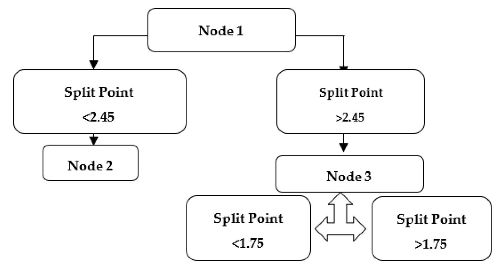
2.1. Single Decision Trees (SDTs)

There are three main components of SDTs: edges, leaves, and terminals. Edges proceed toward the child node. Leaves entail connecting nodes to another node; the terminal node represents the output value following tree construction [43]. SDTs comprise two phases for tree generation. The first phase involves tree growth, whereas the second part involves tree pruning. The data will be constructed in ascending order during tree construction. Tree trimming eliminates or adjusts data that cause noise or have a high entropy level; after pruning the data tree, a regression or classification tree is constructed depending on the given data (continuous or categorical). DTREG [42] will use a variety of variables in a class of variables, including target, predicted, and weight variables. The association between the goal and predicted variables is created in tree building; the weight variable establishes the weight between nodes via edges. The data variables are assigned equal weights if no weight variable is supplied to the data row. If the data variables are continuous, DTREG separates the data based on petal length after randomly selecting data. If the data variables are categorical, the petal width will be used to split the data. The node represents the predicted and desired variables. The splitting variable will be shifted to the child node to continue building the tree. Random data will be separated using regression analysis and the tree technique, as well as misclassification error and probability [22]. Figure 1 depicts the complete schematic diagram of SDTs.
No. of splits = 2(k−1)−1
No. of terminal nodes = 2k

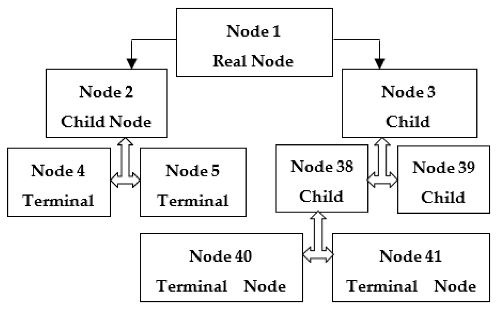
2.2. Decision Tree Forests (DTFs)

The DTFs assign data of desired continuous or categorical variables to the model. Numeric values represent continuous data and alphabetic or character variables represent categorical data. The data are going to be partitioned according to the misclassification error. A misunderstanding of the classification led to the initiation of the investigation into structural dependability. The Monte Carlo simulation, the simplified order reliability method (SORM), and the first-order reliability method (FORM) are examples of strategies or approaches that can be used to estimate the likelihood of a failure occurring. These methods are utilized to determine how successful reliability analysis truly is. A tree will be built for each attribute to show how the attributes are related to one another. The node with the lowest rate of incorrect classification will be the root node, and logarithms incorporating the C 4.5 algorithm will be used to produce splitting from the note node [36].
In Figure 2, the data splitting and error elimination process will continue until either the terminal node is reached or the data misclassification error (ME) at the end of the terminal node becomes zero, at which time further data splitting will end. The output value can be seen on the terminal node generation’s display.
Figure 3 depicts the entire working principle of DTFs.

2.3. Tree Boost (TB)

Jerome H. Friedman is the pioneer stakeholder of this technique [44]. Another name for TB is stochastic gradient boosting and multiple regression trees. The algorithm or working principle is the same as tree forests. The only difference between TB and DTFs is the mode of construction. TB generates trees in a series pattern, whereas DTFs consist of a forest of trees in parallel. It is a technique that enhances accuracy by weighing output values to reduce total prediction error. The general working mechanism of the is shown in Figure 4.

2.4. Multi-Layer Perceptron (MLP)

Most hydrologists and researchers compute rainfall and runoff using artificial neural networks, the most well-known method. ANN consists of three layers: the input layer, the hidden layer, and the output layer. The input layer receives the information. The subsequent layer generates a beautiful link between rainfall data using algorithmic functions and other mathematical techniques. The final layer provides the output value. Jang introduced ANFIS in 1993 [11], consisting of five output interpretation layers. In layer 1, the membership function is used to associate variables with membership while layer 2 consists of nodes that establish a relationship with incoming signals. The third layer locks every node, the fourth layer computes each node’s contribution to the output value, and the last layer provides the result. There are numerous varieties of ANN. MLPNN (multi-layer perceptron neural network) is utilized in hydrology [45]. In Figure 5 and Figure 6, MLPNN is depicted as a network of input; hidden and neuronal output layers are all present. A layer comprises many neurons, each in the preceding layer linked to those in the next layer. Consider the input layer’s output value as the hidden layer’s input value.
Similarly, the hidden layer’s output value will be the output layer’s input value. The neuron transfer function sends neurons between the hidden and output layers. There is no point link between the input and output layers.
The input layer receives the data. All neurons in this layer are linked and use mathematical functions to process data in the buried layer. The output layer receives input from the concealed layer and returns the anticipated value [22,35]. Six external inputs are supplied in the input layer of Figure 6. Each neuron in the input layer interacts with neurons in the layers beneath it. These values can be transmitted using mathematical functions, with the output layer being responsible for interpreting the resulting value.

2.5. Study Area

This study focused on daily precipitation and runoff in the Mangla basin. The Mangla watershed is located at a latitude 33–35° N and longitude 73.62° E. As seen in Figure 7, the Mangla catchment’s demographical borders are in Pakistan and India. It has a drainage area of 165,499.15 km2, making it the second-largest tributary in the world after the Indus basin [22]. The Mangla watershed is situated on the Jhelum River and has a storage capacity of 7.475 MAF and a drainage area of 33,333.15 km2. The runoff of the Jhelum River basin drains into the Mangla watershed. This catchment supplies irrigation and hydropower with water. Six million hectares of land are irrigated from this reservoir as part of a 1000 MW hydroelectric power-producing capability. The Jhelum and its tributaries, Neelam, Poonch, Kanshi, and Naran, make up the Mangla watershed. In the catchment area, precipitation and snowmelt generated runoff, representing the reservoir’s intake. The water stored in various basins, such as the Neelam, Poonch, Kanshi, Jhelum, and Naran basin, will flow to the river Jhelum as runoff at the Mangla catchment.

2.6. Dataset

There are twelve rain gauge stations in the boundary of the Mangla reservoir, as shown in Figure 7. Nine stations are in Pakistan while the remaining are in India. Table 1 contains information about these stations and Figure 7 depicts their location. These rain gauge stations allow us to mimic the runoff generated and dropping into the Jhelum River at the Mangla. The four rain gauge stations are in the Indian territory and cover a broad region for the contribution of runoff from the Mangla basin above the Jhelum River. Data on daily rainfall for 29 years from January 1978 to Dec 2007 from nine stations located in Pakistan is obtained in the Pakistan Metrological Department. The daily rainfall data of four stations outside of Pakistan are obtained from [46]. The rainfall data of these thirteen stations are averaged arithmetically to calculate the point of rainfall over the Basin. The corresponding discharge is the inflow to the Mangla reservoir used in this study.

2.7. Performance Evaluation
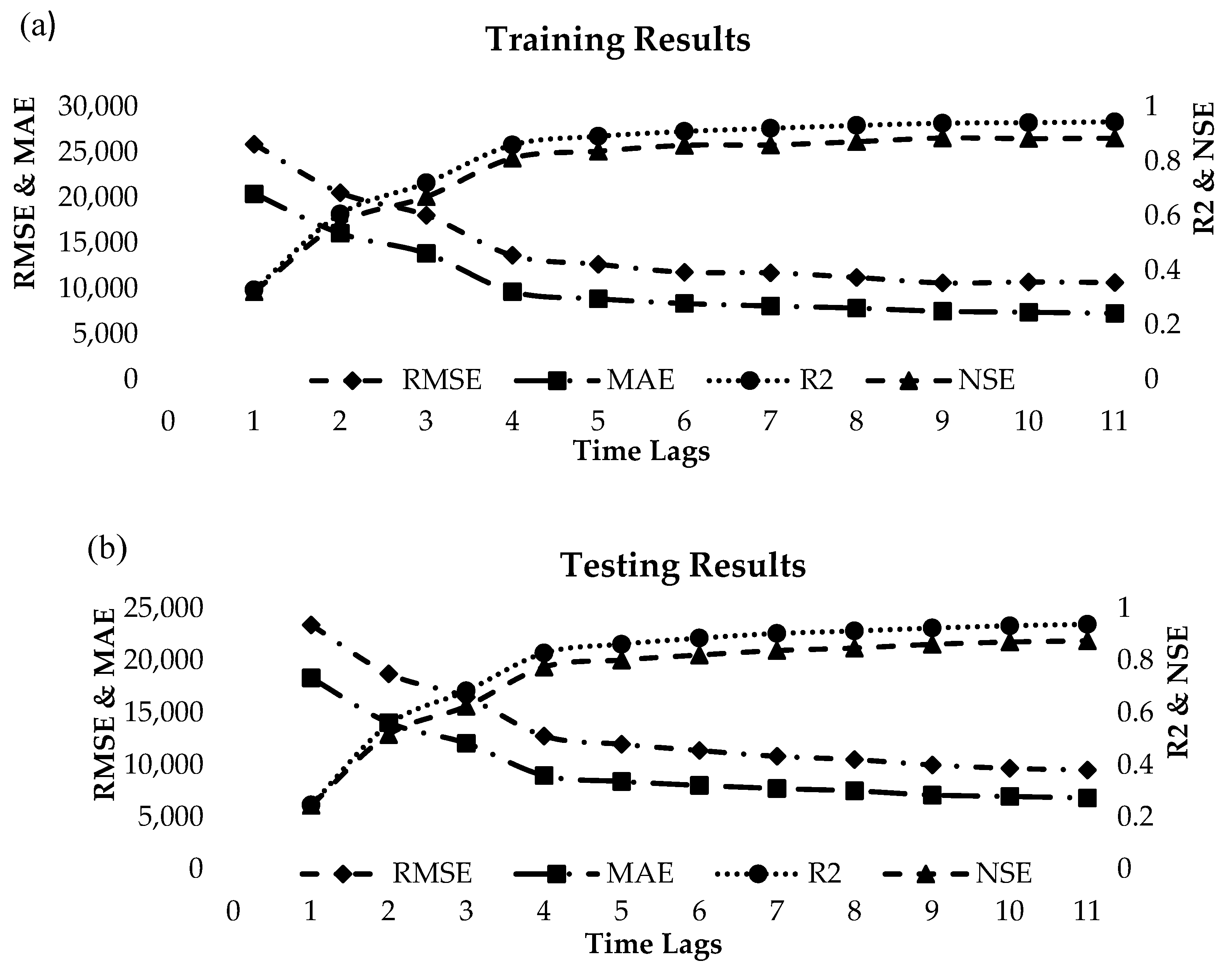
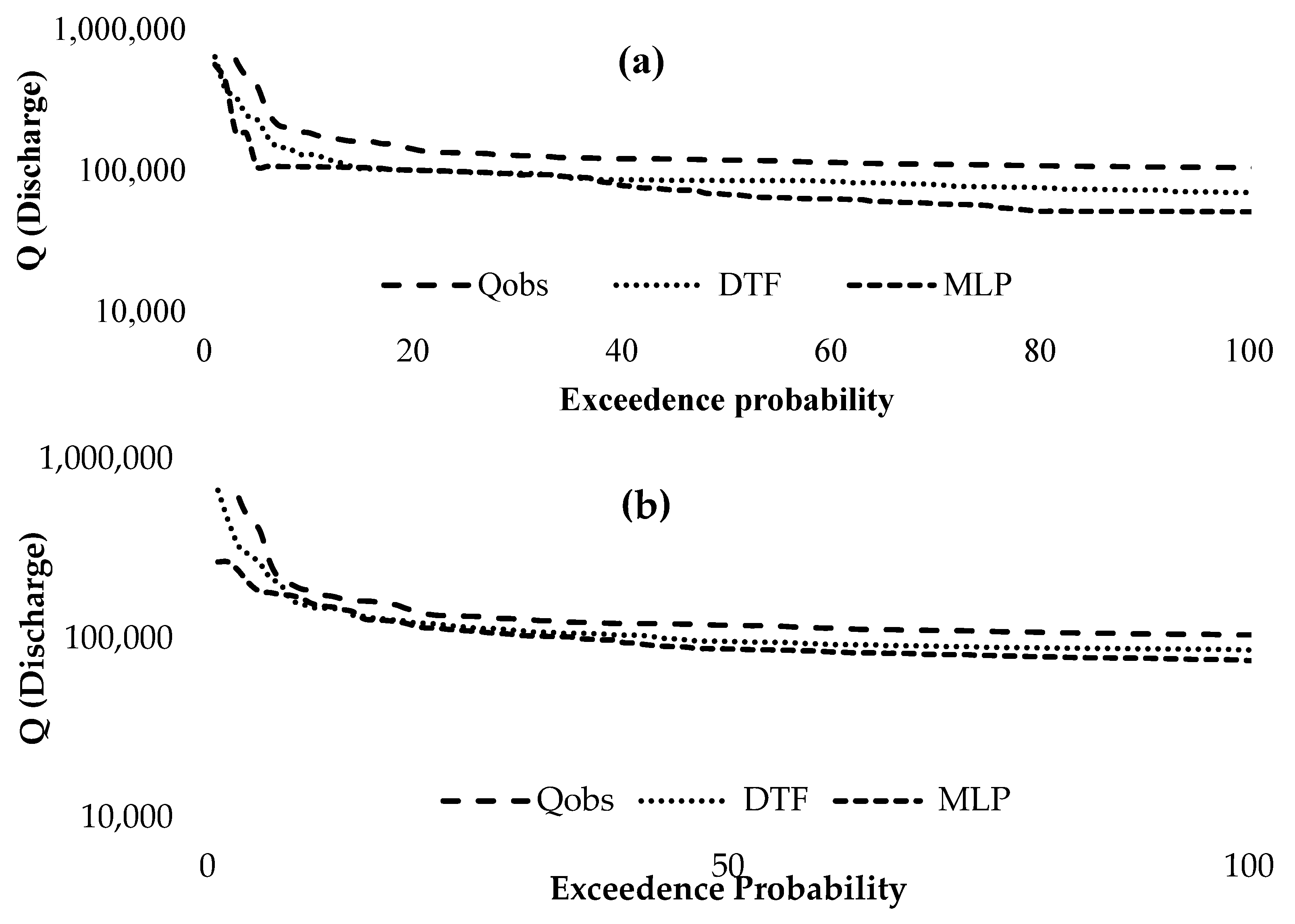
While dealing with some hydrological processes, determining the model’s goodness depends upon various statistical parameters, such as rainfall-runoff modeling. The current study employs four statistical evaluation metrics to determine the model’s goodness. The basic formulas of these four statistical parameters are:
R 2   =   n ( x y ) ( x ) ( y ) n [ x 2 ( x 2 ) ] [ y 2 ( y 2 ) ]
RMSE = ( Q o b s Q p r e ) ^ 2 N
MAE = ( Q p r e Q o b s ) N
NSE = 1 ( Q o b s Q m o d ) ^ 2 ( Q o b s Q a v e ) ^ 2
AIC = mln(RMSE) + 2n
For an efficient correlation between expected and observed values, R2 is between 0 and 1. The model will be considered the most efficient when the correlation coefficient value approaches 1 or is equal to 1. The range of model efficiency RMSE values is between 0 and 1. The better the model, the lower the RMSE number, while the worse the model or data, the higher the RMSE value. Most hydrological studies provide NSE values as percentages [24,47]. In Equation (7), where m is the number of input–output training patterns, n is the number of parameters to be detected and RMSE is the root-mean-square error between the network output and target. The RMSE statistics are predicted to improve when more parameters are introduced to a model, whereas the AIC statistics punish the model for having more parameters and, as a result, tend to produce more parsimonious models [48].

3. Results

The current work aims to simulate the rainfall-runoff process using several methodologies, such as SDTs, TB, and DTFs, and then compare the findings of these models with MLP. This rainfall-runoff modeling uses several rainfall combinations to obtain statistically significant results. The input data employed in this study are the lagging rainfall data, whereas the desired output is the observed inflow into the Mangla reservoir. To forecast current runoff Q(t), the eleven input combinations of lagged precipitation are given in Table 2. Selecting a suitable collection of inputs is essential for accurate data-driven rainfall and runoff forecasting. We employed Akaike’s information criterion (AIC) for the analysis inputs combination and the AIC values of selected input combinations shown in Table 2.
This study uses daily rainfall-runoff data spanning 29 years, beginning in January 1978 and ending in December 2007. The remaining data is utilized for validation and testing, while the first fifteen years of data, beginning in January 1978 and ending in December 1993, are used for training purposes. Lagged rainfall was used as the input data for the rainfall-runoff models, while present discharge served as the model’s desired output. Prediction models were constructed utilizing the four applied approaches of SDTs, DTFs, TB, and MLP. The models’ statistical evaluation is presented in Table 3, Table 4, Table 5, Table 6, Table 7, Table 8, Table 9 and Table 10. During the training and testing of the models, it was observed that the error rate was acceptable and improved from the training to the test process with different input combinations. The error rate was improved as an acceptable value when input combinations were changed from a 1-day lag to a 10-day lag. Overall, the percent of improvement for DTFs in terms of R2 was 57%; for RMSE, it was found to be a 17% improvement.
Table 3 demonstrates that DTF was superior to the other three methods. The R2 and NSE values for DTF training and testing range between 0.24 to 0.32. The RMSE and MAE are approximately 24,000 and 19,000 cumecs. R2 and NSE values for SDT are between 0.10 and 0.11 to 1 for training and testing. The figures for RMSE and MAE range between 27,000 and 20,000 cumecs. R2 and NSE range between 0.15 and 0.10 for TB, whereas the other statistical measures, RMSE, and MAE, range between 26,000 and 19,000 cumecs. The typical technique MLP has a training and testing value of 0.15 for both R2 and NSE.
RMSE and MAE performance for MLP ranges between 25,000 and 20,000 cumecs. In addition, Table 3 demonstrates that the performance parameters of TB and MLP are nearly identical. SDT’s performance is underrated in comparison to the other three approaches. The bold results from Table 3, Table 4, Table 5, Table 6, Table 7, Table 8, Table 9 and Table 10 shows the best overall outputs of models applied in rainfall runoff prediction. In a manner analogous to Table 3, the performance of the DTFs is superior to that of the other three applied models, while the performance of the TB and MLP is comparable. Table 4 reveals that the values for R2 and NSE for the DTFs fall in the range of 0.5 to 0.6, while the values calculated for RMSE and MAE are approximately 14,000 to 20,000 cumecs. The values of R2 and NSE for SDTs are both 0.20, regardless of whether the model is being trained or tested, whereas the values of RMSE and MAE range between 25,000 and 19,000 cumecs. The TB values for R2 and NSE are 0.20 and 0.18, respectively. RMSE and MAE both perform at a level of 25,000 to 18,000 cumecs. Both the training and testing phases of the MLP have R2 and NSE values of 0.17 and 0.18, respectively. In the case of MLP, the performance evaluation of RMSE and MAE ranges from around 26,000 to 20,000 cumecs. All these results from Table 4 indicate that MLP is less efficient for analyzing runoff when a combination of the three is used. Table 5 shows that the values of R2 and NSE are determined within the range of 0.6 to 0.7 for both training and validation for the DTFs. RMSE and MAE both have values that range between 16,000 and 12,000 cumecs. The values of R2 and NSE are the same, with a value of 0.20, for both the training and the testing phases. RMSE and MAE both have performances that fall somewhere in the range of 25,000 to 18,000 cumecs. For TB, the values for R2 and NSE range from 0.21 to 0.19 for training and testing analyses, whereas the values range from around 25,000 to 20,000 cumecs for RMSE and MAE. Table 8 shows that the values of R2 and NSE for DTFs range from 0.86 to 0.81, while RMSE and MAE are between 13,000 and 9000 cumecs. SDTs show 0.25 for R2 and NSE, but 25,000 and 19,000 cumecs for RMSE and MAE. TB’s training and testing NSE and R2 are 0.23 and 0.18, respectively. RMSE and MAE for TB ranges from 25,000 and 18,000 cumecs. MLP has the same values, 0.19 for R2, NSE, and 25,000 and 19,000 cumecs for RMSE and MAE. The findings in Table 7 indicate that the DTF is a more effective solution than SDT, TB, and MLP. The training and testing stages produce R2 and NSE values for the DTF in the range of 0.89 and 0.83, while the RMSE and MSE values produce 13,000 and 9000 cumecs, respectively. In the SDT, 0.25 is specified for R2, and the exact value is specified for NSE. RMSE and MAE are between 25,000 and 19,000 cumecs. R2 is found to be 0.26 using the TB technique, and NSE is 0.27. The final RMSE and MAE values fall somewhere in a range that goes from 24,000 to 17,000 cumecs. The exact value of 0.17 is shown for MLP’s R2 and NSE. In contrast, RMSE and MAE range from 20,000 and 25,000 cumecs, respectively. Table 8 shows that R2 and NSE for DTFs are between 0.90 and 0.80. RMSE and MAE are 12,000 and 9000 cumecs. SDTs and TB have a 0.25 square correlation and NSE. RMSE and MAE are 250,000 and 180,000 cumecs. 0.20 is MLP’s R2 and NSE. RMSE and MAE range from 25,000 to 19,000 cumecs. MLP is underestimated compared to DTFs, TB, and SDTs. MLP has a lower potential than other techniques. Table 9 reveals that the R2 and NSE values for DTFs are in the region of 0.9 to 0.8, giving it an advantage over TB, SDTs, and MLP. It is evidenced by the fact that DTFs come out on top. The results for RMSE and MAE range between 10,000 and 8000 cumecs. R2 and NSE have 0.25 and 0.27 for SDTs, whereas RMSE and MAE have 25,000 and 17,000 cumecs, respectively. TB has an R2 value of 0.35 and an NSE value of 0.30. Its RMSE value is 24,000 cumecs and its MAE value is 16,000 cumecs. The minimum likelihood proportionate has the lowest value of any statistical parameter. These are the results for R2, NSE, RMSE, and MAE: 0.20, 0.18, 26,000, and 18,000 cumecs, respectively. The DTFs models were the most accurate based on the R2, and NSE values lie between 0.9 and 0.8, as shown in Table 10. The RMSE and the MAE come in at 10,000 cumecs and 7000 cumecs, respectively. R2 values of 0.30 and NSE values of 0.27 are comparable for SDTs and TB, whereas RMSE values of 24,000 cumecs and MAE values of 17,000 cumecs are reported for each. The MLP model has a value of 0.19 for R2 and a comparable amount for NSE. However, the RMSE value is 25,000 cumecs and the MAE value is 19,000 cumecs.
Figure 8a,b depicts the performance parameters R2, NSE, MAE, and RMSE for each input combination for the best DTFs model to examine the effect of the previously mentioned input combinations.
Figure 8a demonstrates the variation in R2 across input combinations. Figure 8a shows an increase in R2 values from input combination 1 with a single P(t) precipitation value to input combination 4, which has P(t), P(t-1), P(t-2), and P(t-3) precipitation data, followed by a constant value. Figure 8b shows a similar pattern for NSE fluctuations. Similarly, Figure 8a,b illustrates the fluctuation of RMSE and MAE, respectively, with selected input combination changes. (c) depicts the overall RMSE and MAE values. Figure 8a,b demonstrates a significant reduction in error values from input combinations up to the input combination, which is consistent with the R2 and NSE values (4). According to the findings, it is possible to assert that the precipitation P(t), P(t-1), P(t-2), and P(t-3) contain complete data about the watershed’s hydrological signature and that there is no vital information hidden in the lag precipitation data. This assertion can be supported by stating that the lag precipitation data do not contain any relevant information.
The flow duration curves (FDC) in Figure 9 were developed to test the efficacy of developed models in projecting low, medium, and high flows. Figure 9a–d are FDCs generated with various combinations of precipitation and lag precipitation series, such as 1-day precipitation, lag-3-day precipitation, lag-5-day precipitation, lag-8-day precipitation, and lag-10-day precipitation, respectively. The flows on these FDCs can be classed as low, medium, or high. If the flow range with exceedance probability is between 0 and 10, the flow is classified as high. If it is from 11 to 89, the flow is classified as medium, which further separates into two classes: low-medium if the flow ranges from 11 to 49, and high-medium if the flow runs between 50 and 89. The discharge is below the 50th percentile when it exceeds 89 [15]. It can be shown from Figure 9a that DTFs and MLP both underestimate the observed discharge for all three high, medium, and low flows. Figure 9b illustrates that MLP and DTFs tie for high and high medium flow with observed discharge. Figure 9c represents DTFs and MLP, which are comparable for high and medium flow. MLP underestimates the observed discharge in the region of low flow and low, medium flow. Figure 9d shows that DTFs capture the high, medium, and low flow with observed discharge better than MLP, and the last Figure 9e directs the best relationship with observed discharge for DTFs, including high, medium, and low flow.

4. Discussion

The DTF was the best technique in the training and testing applied soft computing techniques, such as MLP, SDTs, DTFs, and TB. The average values of R2 and NSE discovered during the training and testing of models were found to be more than other techniques, as shown in Table 5, Table 6, Table 7, Table 8, Table 9 and Table 10. The percent of improvement in terms of R2 and RMSE in the outputs of DTFs up to the maximum value of 57% and 17%, respectively, compared to other techniques. Many researchers quoted that results from DTFs are generally equal to 1 and many others [22,49,50]. R2 is one of the most significant model evaluation criteria that many hydrologists and researchers have found and utilized for predicting and forecasting the behavior of various hydrological cycle components [30]. The RMSE findings of all the different input combinations demonstrated that the DTFs have a higher ability to predict rainfall and runoff than SDTs and TB while the models are being trained and tested. The reduced value of the root-mean-square error (RMSE) demonstrates that the model is accurate [51]. DTFs and SDTs were previously used for streamflow forecasting and showed good potential [22]. In Figure 8a,b, TB and SDTs demonstrated the most effective results of 1.00 in training modeling techniques at all stations, according to the NSE results for both train and test cases of soft computing techniques. SDTs, TB, and MLP showed less efficient results. The higher NSE value shows the models’ efficiency [52]. Figure 8a,b shows that the DTF has better runoff prediction than SDT and TB, according to RMSE values. DTF is a more effective MLP than the conventional one [22]. A smaller value of the RMSE indicates the model’s fitness [53]. So, the DTFs are the most effective technique for rainfall and runoff prediction for the Mangla watershed, according to NSE results previously mentioned by [54]. Figure 9 shows that hydrographs of the low, medium, and high streams were made using soft computing techniques such as SDTs, DTFs, and MLP to analyze their capability. These techniques were used to create the hydrographs. DTFs have good potential for predicting runoff. For the evaluation of catchment features, the lower and upper regions of the FDCs are essential parts. The low flow component of the FDC indicates how well the catchment can support itself during hot and dry weather. The catchment is likely to have the flood regime indicated by the high flow portion [7,15].
In contrast to the considerably smoother curves towards the upper portion, which are due to floods caused by snowmelt, steep curves show floods mostly driven by rain in small catchments. The flat curves in the low flow region represent flows resulting from either natural or artificial streamflow [15]. SDTs, DTFs, TB, and MLP were tested in the observed hydrographs with high, medium, and low flows. Numerous investigations from the past have shown that the FDCs’ demonstrations of exceedance probability versus the simulated and observed flows that represent the specified discharges were surpassed during the designated period [55,56]. When the flow is between or equal to 1 and 10 percent of the time, it is deemed to be high. The flow rate is deemed high when it falls within 1 to 10 percent of the period.
Similarly, flows are considered medium flows from the 11th to the 89th percentile and low flows from the 90th to the 100th percentile. The flow from the 11th to the 49th percentile is considered a high-medium flow, while the flow from the 50th to the 89th percentile is considered a low-medium flow [56]. Compared to other FDCs of SDTs, TB, and MLP, DTFs are a better method for medium-high and high percentile flows and correlate with the observed flow duration curve. The FDCs of TB bond with observed flow FDCs superior to others for low and medium-low percentile flows. The FDCs of all Mangla watershed stations observed and predicted by various soft computing approaches revealed that DTFs outperformed. DTFs are better than other techniques in forecasting medium-high and high discharges, while TB is better at estimating low and medium-low discharges over the long term. SDTs can predict high-flow runoffs.

5. Conclusions

This study evaluates the performance of SDTs, DTFs, TB, and MLP for rainfall-runoff analysis. The analysis and observations show that DTFs are superior to all other data-driven approaches, including SDTs, TB, and MLP. In contrast, based on the outcomes of performance evaluation criteria, DTFs are assessed as the most successful advanced soft computing approach among other applied approaches. In addition, SDTs and TB have fared better in yearly streamflow forecasts. However, the SDTs were deemed the most effective approach for the Mangla catchment. The accuracy between observed and forecast runoff in the current catchment was evaluated using FDCs. The results of FDCs revealed that the DTFs was a superior method for medium-high and high-percentile flows and had stronger correlations with the FDC of observed flow than other methods. MLP is frequently compared to DTFs because both methods model data with nonlinear connections between variables and manage interactions. However, neural networks have certain disadvantages in comparison to DTFs. The MLP model is not easily comprehensible. When examining DTFs, TB, and SDTs, it is straightforward to observe that an initial variable splits the data into two categories, and subsequently, further variables separate the following child groups. This information is quite helpful for the researcher attempting to comprehend the data’s nature.
Soft computing approaches have limitations that focus on data and strive to extract variables and relations from raw data, yielding more accurate answers without using analytical laws and equations. Many issues remain; in some cases, physical principles are not fulfilled. It can be utilized in the forecasting of numerous different hydrological processes, including evapotranspiration, rainfall-runoff, and sediment transport. This study further investigates that DTFs have a higher potential for rainfall-runoff analysis.

Author Contributions

Conceptualization, U.W.H. and M.S.; methodology, R.A. and M.W.; software, R.A. and M.W.; validation, M.W., P.T.H. and H.A.L.; formal analysis, R.A.; investigation, R.A., U.W.H. and M.W.; Validation P.V. and P.T.H., Software, P.T.H. and H.A.L. resources, M.S. and U.W.H.; data curation, M.W. and R.A.; writing—original draft preparation, R.A. and M.W.; visualization, R.A., H.A.L. and P.T.H.; supervision, U.W.H. and M.S.; project administration, M.S.; funding acquisition, P.V. and U.W.H., Writing–review & editing, U.W.H., P.V., M.F. and S.A. All authors have read and agreed to the published version of the manuscript.

Funding

This research received no external funding.

Data Availability Statement

Data used to support the study’s findings can be obtained from the corresponding author upon request.

Acknowledgments

All the authors thank King Mongkut’s University of Technology Thonburi, Bangkok, Thailand and Bahauddin Zakariya University, Multan, Pakistan, for their support and technical help.

Conflicts of Interest

The authors declare no conflict of interest.

Abbreviations

TBTree Boost
DTFsDecision tree forests
SDTsSingle decision trees
MLPMultilayer perceptron
RMSERoot means square error
MAEMean absolute error
R2Coefficient of determination
NSENash–Sutcliffe efficiency
FDCsFlow duration curves
ANNArtificial neural network
ANFISAdaptive neuro-fuzzy inference system
GPGenetic programming
GEPGene expression programming
SVMSupport vector machine
BPABack-propagation algorithm
RGAReal-coded genetic algorithm
SOMSelf-organizing map
MCSMonte Carlo simulation
SORMSimplified order reliability method
FORMFirst-order reliability method
MEmisclassification error
km2Square kilometers (area)
MAFMillion acre feet (storage capacity)
MWMegawatts (electric power)
°CDegrees Celsius (temperature)
InchesPrecipitation

References

  1. Nawaz, Z.; Li, X.; Chen, Y.; Guo, Y.; Wang, X. Temporal and Spatial Characteristics of Precipitation and Temperature in Punjab, Pakistan. Water 2019, 11, 1916. [Google Scholar] [CrossRef] [Green Version]
  2. Fahad, S.; Wang, J. Climate change, vulnerability, and its impacts in rural Pakistan: A review. Environ. Sci. Pollut. Res. 2020, 27, 1334–1338. [Google Scholar] [CrossRef] [PubMed]
  3. Asadi, S.; Shahrabi, J.; Abbaszadeh, P.; Tabanmehr, S. A new hybrid artificial neural networks for rainfall–runoff process modeling. Neurocomputing 2013, 121, 470–480. [Google Scholar] [CrossRef]
  4. Waqas, M.; Saifullah, M.; Hashim, S.; Khan, M.; Muhammad, S. Evaluating the Performance of Different Artificial Intelligence Techniques for Forecasting: Rainfall and Runoff Prospective. In Weather Forecasting; IntechOpen: London, UK, 2021; p. 23. [Google Scholar]
  5. Gholami, V.; Sahour, H. Simulation of rainfall-runoff process using an artificial neural network (ANN) and field plots data. Theor. Appl. Climatol. 2022, 147, 87–98. [Google Scholar] [CrossRef]
  6. Solomatine, D.; See, L.M.; Abrahart, R.J. Data-driven modelling: Concepts, approaches and experiences. In Practical Hydroinformatics; Abrahart, R.J., See, L.M., Solomatine, D.P., Eds.; Springer: Berlin/Heidelberg, Germany, 2009; pp. 17–30. [Google Scholar]
  7. Shoaib, M.; Shamseldin, A.Y.; Melville, B.W.; Khan, M.M. A comparison between wavelet based static and dynamic neural network approaches for runoff prediction. J. Hydrol. 2016, 535, 211–225. [Google Scholar] [CrossRef]
  8. Verma, R. ANN-based Rainfall-Runoff Model and Its Performance Evaluation of Sabarmati River Basin, Gujarat, India. Water Conserv. Sci. Eng. 2022, 1–8. [Google Scholar] [CrossRef]
  9. Nourani, V.; Baghanam, A.H.; Adamowski, J.; Kisi, O. Applications of hybrid wavelet–Artificial Intelligence models in hydrology: A review. J. Hydrol. 2014, 514, 358–377. [Google Scholar] [CrossRef]
  10. Fama, E.F.; French, K.R. The Cross-Section of Expected Stock Returns. J. Financ. 1992, 47, 427–465. [Google Scholar] [CrossRef]
  11. Jang, J.-S.R. ANFIS: Adaptive-Network-Based Fuzzy Inference System. IEEE Trans. Syst. Man Cybern. 1993, 23, 665–685. [Google Scholar] [CrossRef]
  12. Koza, J.R. Evolution of subsumption using genetic programming. In Toward a Practice of Autonomous Systems: Proceedings of the First European Conference on Artificial Life; MIT Press: Cambridge, MA, USA, 1992. [Google Scholar]
  13. Savic, D.A.; Walters, G.A.; Davidson, J.W. A genetic programming approach to rainfall-runoff modelling. Water Resour. Manag. 1999, 13, 219–231. [Google Scholar] [CrossRef]
  14. Joachims, T. Text categorization with Support Vector Machines: Learning with many relevant features. In Machine Learning: ECML-98; Springer: Berlin/Heidelberg, Germany, 1998; pp. 137–142. [Google Scholar]
  15. Shoaib, M.; Shamseldin, A.Y.; Melville, B.W. Comparative study of different wavelet based neural network models for rainfall–runoff modeling. J. Hydrol. 2014, 515, 47–58. [Google Scholar] [CrossRef]
  16. Zounemat-Kermani, M.; Kisi, O.; Rajaee, T. Performance of radial basis and LM-feed forward artificial neural networks for predicting daily watershed runoff. Appl. Soft Comput. 2013, 13, 4633–4644. [Google Scholar] [CrossRef]
  17. Srinivasulu, S.; Jain, A. A comparative analysis of training methods for artificial neural network rainfall–runoff models. Appl. Soft Comput. 2006, 6, 295–306. [Google Scholar] [CrossRef]
  18. Setiono; Hadiani, R. Analysis of Rainfall-runoff Neuron Input Model with Artificial Neural Network for Simulation for Availability of Discharge at Bah Bolon Watershed. Procedia Eng. 2015, 125, 150–157. [Google Scholar] [CrossRef] [Green Version]
  19. Elsafi, S.H. Artificial Neural Networks (ANNs) for flood forecasting at Dongola Station in the River Nile, Sudan. Alex. Eng. J. 2014, 53, 655–662. [Google Scholar] [CrossRef]
  20. Farajzadeh, J.; Fard, A.F.; Lotfi, S. Modeling of monthly rainfall and runoff of Urmia lake basin using "feed-forward neural network" and "time series analysis" model. Water Resour. Ind. 2014, 7–8, 38–48. [Google Scholar] [CrossRef] [Green Version]
  21. Napolitano, G.; See, L.; Calvo, B.; Savi, F.; Heppenstall, A. A conceptual and neural network model for real-time flood forecasting of the Tiber River in Rome. Phys. Chem. Earth Parts A/B/C 2010, 35, 187–194. [Google Scholar] [CrossRef]
  22. Waqas, M.; Shoaib, M.; Saifullah, M.; Naseem, A.; Hashim, S.; Ehsan, F.; Ali, I.; Khan, A. Assessment of Advanced Artificial Intelligence Techniques for Streamflow Forecasting in Jhelum River Basin. Pak. J. Agric. Res. 2021, 33, 580–598. [Google Scholar] [CrossRef]
  23. Rajurkar, M.; Kothyari, U.; Chaube, U. Modeling of the daily rainfall-runoff relationship with artificial neural network. J. Hydrol. 2004, 285, 96–113. [Google Scholar] [CrossRef]
  24. Shamseldin, A.Y. Application of a neural network technique to rainfall-runoff modelling. J. Hydrol. 1997, 199, 272–294. [Google Scholar] [CrossRef]
  25. Shin, M.-J.; Guillaume, J.H.A.; Croke, B.F.W.; Jakeman, A.J. A review of foundational methods for checking the structural identifiability of models: Results for rainfall-runoff. J. Hydrol. 2015, 520, 1–16. [Google Scholar] [CrossRef]
  26. Tokar, A.S.; Johnson, P.A. Rainfall-Runoff Modeling Using Artificial Neural Networks. J. Hydrol. Eng. 1999, 4, 232–239. [Google Scholar] [CrossRef]
  27. Wu, C.L.; Chau, K.W.; Fan, C. Prediction of rainfall time series using modular artificial neural networks coupled with data-preprocessing techniques. J. Hydrol. 2010, 389, 146–167. [Google Scholar] [CrossRef] [Green Version]
  28. Devak, M.; Dhanya, C.; Gosain, A. Dynamic coupling of support vector machine and K-nearest neighbour for downscaling daily rainfall. J. Hydrol. 2015, 525, 286–301. [Google Scholar] [CrossRef]
  29. He, Z.; Wen, X.; Liu, H.; Du, J. A comparative study of artificial neural network, adaptive neuro fuzzy inference system and support vector machine for forecasting river flow in the semiarid mountain region. J. Hydrol. 2014, 509, 379–386. [Google Scholar] [CrossRef]
  30. Kisi, O.; Cimen, M. A wavelet-support vector machine conjunction model for monthly streamflow forecasting. J. Hydrol. 2011, 399, 132–140. [Google Scholar] [CrossRef]
  31. Kundu, S.; Khare, D.; Mondal, A. Future changes in rainfall, temperature and reference evapotranspiration in the central India by least square support vector machine. Geosci. Front. 2017, 8, 583–596. [Google Scholar] [CrossRef]
  32. Noori, R.; Karbassi, A.R.; Moghaddamnia, A.; Han, D.; Zokaei-Ashtiani, M.H.; Farokhnia, A.; Gousheh, M.G. Assessment of input variables determination on the SVM model performance using PCA, Gamma test, and forward selection techniques for monthly stream flow prediction. J. Hydrol. 2011, 401, 177–189. [Google Scholar] [CrossRef]
  33. Rasouli, K.; Hsieh, W.W.; Cannon, A.J. Daily streamflow forecasting by machine learning methods with weather and climate inputs. J. Hydrol. 2012, 414–415, 284–293. [Google Scholar] [CrossRef]
  34. Keskin, M.E.; Taylan, D.; Terzi, Ö. Adaptive neural-based fuzzy inference system (ANFIS) approach for modelling hydrological time series. Hydrol. Sci. J. 2006, 51, 588–598. [Google Scholar] [CrossRef]
  35. Shoaib, M.; Shamseldin, A.Y.; Melville, B.W.; Khan, M.M. Runoff forecasting using hybrid Wavelet Gene Expression Programming (WGEP) approach. J. Hydrol. 2015, 527, 326–344. [Google Scholar] [CrossRef]
  36. Quinlan, J.R. Simplifying decision trees. Int. J. Man-Mach. Stud. 1987, 27, 221–234. [Google Scholar] [CrossRef] [Green Version]
  37. Preis, A.; Ostfeld, A. A coupled model tree–genetic algorithm scheme for flow and water quality predictions in watersheds. J. Hydrol. 2008, 349, 364–375. [Google Scholar] [CrossRef]
  38. Etemad-Shahidi, A.; Mahjoobi, J. Comparison between M5′ model tree and neural networks for prediction of significant wave height in Lake Superior. Ocean Eng. 2009, 36, 1175–1181. [Google Scholar] [CrossRef]
  39. Xu, M.; Watanachaturaporn, P.; Varshney, P.K.; Arora, M.K. Decision tree regression for soft classification of remote sensing data. Remote Sens. Environ. 2005, 97, 322–336. [Google Scholar] [CrossRef]
  40. Deo, R.C.; Kisi, O.; Singh, V.P. Drought forecasting in eastern Australia using multivariate adaptive regression spline, least square support vector machine and M5Tree model. Atmos. Res. 2017, 184, 149–175. [Google Scholar] [CrossRef] [Green Version]
  41. Clay, D.E.; Alverson, R.; Johnson, J.M.; Karlen, D.L.; Clay, S.; Wang, M.Q.; Bruggeman, S.; Westhoff, S. Crop Residue Management Challenges: A Special Issue Overview. Agron. J. 2019, 111, 1–3. [Google Scholar] [CrossRef] [Green Version]
  42. Sherrod, P.H. DTREG Predictive Modeling Software; DTREG: Brentwood, TN, USA, 2003; Available online: http://www.dtreg.com (accessed on 30 December 2003).
  43. Sherrod, P. Classification and Regression Trees and Support Vector Machines for Predictive Modeling and Forecasting; DTREG: Brentwood, TN, USA, 2006; Available online: http://www.DTREG.com/DTREG.pdf (accessed on 30 December 2006).
  44. Friedman, J.; Hastie, T.; Tibshirani, R. Additive logistic regression: A statistical view of boosting (With discussion and a rejoinder by the authors). Ann. Stat. 2000, 28, 337–407. [Google Scholar] [CrossRef]
  45. McGarry, K.; Wermter, S.; MacIntyre, J. Knowledge extraction from radial basis function networks and multilayer perceptrons. In Proceedings of the IJCNN’99, International Joint Conference on Neural Networks (Cat. No.99CH36339), Washington, DC, USA, 10–16 July 1999; IEEE: Piscataway, NJ, USA, 1999. [Google Scholar]
  46. Mahmood, R.; Babel, M.S. Evaluation of SDSM developed by annual and monthly sub-models for downscaling temperature and precipitation in the Jhelum basin, Pakistan and India. Theor. Appl. Climatol. 2012, 113, 27–44. [Google Scholar] [CrossRef]
  47. Jacquin, A.P.; Shamseldin, A.Y. Development of rainfall–runoff models using Takagi–Sugeno fuzzy inference systems. J. Hydrol. 2006, 329, 154–173. [Google Scholar] [CrossRef]
  48. Akaike, H. A new look at the statistical model identification. IEEE Trans. Autom. Control 1974, 19, 716–723. [Google Scholar] [CrossRef]
  49. Tayyab, M.; Ahmad, I.; Sun, N.; Zhou, J.; Dong, X. Application of Integrated Artificial Neural Networks Based on Decomposition Methods to Predict Streamflow at Upper Indus Basin, Pakistan. Atmosphere 2018, 9, 494. [Google Scholar] [CrossRef] [Green Version]
  50. Sharma, V.; Mishra, V.D.; Joshi, P.K. Implications of climate change on streamflow of a snow-fed river system of the Northwest Himalaya. J. Mt. Sci. 2013, 10, 574–587. [Google Scholar] [CrossRef] [Green Version]
  51. Nash, J.E.; Sutcliffe, J.V. River flow forecasting through conceptual models part I—A discussion of principles. J. Hydrol. 1970, 10, 282–290. [Google Scholar] [CrossRef]
  52. Chai, T.; Draxler, R.R. Root mean square error (RMSE) or mean absolute error (MAE)?—Arguments against avoiding RMSE in the literature. Geosci. Model Dev. 2014, 7, 1247–1250. [Google Scholar] [CrossRef] [Green Version]
  53. Archer, D.; Fowler, H. Using meteorological data to forecast seasonal runoff on the River Jhelum, Pakistan. J. Hydrol. 2008, 361, 10–23. [Google Scholar] [CrossRef]
  54. Babur, M.; Babel, M.S.; Shrestha, S.; Kawasaki, A.; Tripathi, N.K. Assessment of Climate Change Impact on Reservoir Inflows Using Multi Climate-Models under RCPs—The Case of Mangla Dam in Pakistan. Water 2016, 8, 389. [Google Scholar] [CrossRef] [Green Version]
  55. Hayat, H.; Akbar, T.A.; Tahir, A.A.; Hassan, Q.K.; Dewan, A.; Irshad, M. Simulating Current and Future River-Flows in the Karakoram and Himalayan Regions of Pakistan Using Snowmelt-Runoff Model and RCP Scenarios. Water 2019, 11, 761. [Google Scholar] [CrossRef]
  56. Searcy, J.K. Flow-Duration Curves; US Government Printing Office: Washington, DC, USA, 1959. [Google Scholar]
Figure 1. Basic structure of decision tree.
Water 14 03286 g001
Figure 2. Flow sheet diagram of decision tree forests.
Water 14 03286 g002
Figure 3. Working principle of decision tree.
Water 14 03286 g003
Figure 4. Flow sheet diagram of Tree Boost technique.
Water 14 03286 g004
Figure 5. Flow sheet diagram of MLP.
Water 14 03286 g005
Figure 6. Multi-layer perceptron neural networks.
Water 14 03286 g006
Figure 7. Mangla catchment study area.
Water 14 03286 g007
Figure 8. (a,b) Impact of input combinations on the performance.
Water 14 03286 g008
Figure 9. (a) FDCs between DTF, MLP and Qobs with input combination R(t). (b) FDCs between DTF, MLP and Qobs with input combination R(t-3). (c) FDCs between DTF, MLP and Qobs with input combination R(t-5). (d) FDCs between DTF, MLP and Qobs with input combination R(t-8). (e) FDCs between DTF, MLP and Qobs with input combination R(t-10).
Water 14 03286 g009aWater 14 03286 g009b
Table 1. Statistics of rainfall stations in the Mangla catchment.
Name of StationElevation (MSL) in MetersLatitudeLongitudeMean Yearly Precipitation (Inches)Mean Yearly Temperature (°C)Country
Naran240934.909° N73.6507° E1.8319Pakistan
Balakot97534.548° N73.3532° E48.725.1Pakistan
Muzaffarabad67934.359° N73.47105° E45.6727.6Pakistan
Gharidopatta81734.225° N73.6154° E3.8525.9Pakistan
Murree2291.233.907° N73.3943° E5.9117.7Pakistan
Plandri140033.715° N73.6861° E5.9121.8Pakistan
Kotli300033.518° N73.9022° E5.4828.5Pakistan
Rawlakot163833.866° N73.7666° E19.9924.7Pakistan
Kupwaara152234.033° N74.266° E42.0013.9India
Qazigund167033.624° N75.145° E3.3027.0India
Gulmerg265034.05° N74.38° E67.14.1India
Sirinagar500034.083° N74.797° E32.511.8India
Table 2. The information criteria statistics of input combinations are used for runoff estimation.
Input Combinations AIC
P(t) 4.5432
P(t), P(t-1) 4.2015
P(t), P(t-1), P(t-2) 4.1534
P(t), P(t-1), P(t-2), P(t-3) 3.9812
P(t), P(t-1), P(t-2), P(t-3), P(t-4) 3.9678
P(t), P(t-1), P(t-2), P(t-3), P(t-4), P(t-5) 3.9561
P(t), P(t-1), P(t-2), P(t-3), P(t-4), P(t-5), P(t-6) 3.8911
P(t), P(t-1), P(t-2), P(t-3), P(t-4), P(t-5), P(t-6), P(t-7) 3.6582
P(t), P(t-1), P(t-2), P(t-3), P(t-4), P(t-5), P(t-6), P(t-7), P(t-8)3.5121
P(t), P(t-1), P(t-2), P(t-3), P(t-4), P(t-5), P(t-6), P(t-7), P(t-8), P(t-9) 3.3140
P(t), P(t-1), P(t-2), P(t-3), P(t-4), P(t-5), P(t-6), P(t-7), P(t-8), P(t-9), P(t-10) 3.1480
Table 3. Training and testing results with Q(t) of different data mining techniques.
Training Results with P(t)Testing Results with P(t)
ModelR2NSERMSEMAEModelR2NSERMSEMAE
DTFs0.3290.32225,905.66820,441.804DTFs0.2470.24523,431.45218,356.359
SDTs0.0721.00030,319.63221,709.896SDTs0.1160.11625,354.22119,403.642
TB0.1690.16428,804.12920,771.767TB0.1180.09325,975.93318,769.243
MLP0.1450.14429,107.89321,653.686MLP0.1630.16324,671.50919,676.838
Table 4. Training and testing results with Q(t-1) of different data mining techniques.
Training Results with P(t-1)Testing Results with P(t-1)
ModelR2NSERMSEMAEModelR2NSERMSEMAE
DTFs0.6070.57320,552.85916,087.144DTFs0.5550.51718,743.68614,051.887
SDTs0.2830.28326,655.35520,296.326SDTs0.1430.14324,957.49218,966.122
TB0.2470.23427,574.58919,787.896TB0.1790.15724,902.51717,934.826
MLP0.2020.20128,125.94221,264.919MLP0.1500.14924,873.70819,182.440
Table 5. Training and testing results with Q(t-2) of different data mining techniques.
Training Results with P(t-2)Testing Results with P(t-2)
ModelR2NSERMSEMAEModelR2NSERMSEMAE
DTFs0.7210.67018,066.61813,873.521DTFs0.6840.62516,512.01412,073.647
SDTs0.3070.30726,196.09719,778.782SDTs0.1800.18024,422.02118,304.985
TB0.2540.24227,432.89319,339.867TB0.1850.15924,930.98917,685.465
MLP0.2140.21427,899.40520,915.020MLP0.1380.13725,058.22219,672.974
Table 6. Training and testing results with Q(t-3) of different data mining techniques.
Training Results with P(t-3)Testing Results with P(t-3)
ModelR2NSERMSEMAEModelR2NSERMSEMAE
DTFs0.8610.81213,654.8079663.240DTFs0.8290.77612,776.1578996.971
SDTs0.3120.31226,105.99119,558.401SDTs0.1840.18424,360.68918,264.990
TB0.2570.24627,367.76219,095.066TB0.2030.16724,850.15317,518.771
MLP0.2170.21727,850.55020,693.155MLP0.1640.16024,717.33519,418.675
Table 7. Training and testing results with Q(t-4) of different data mining techniques.
Training Results with P(t-4)Testing Results with P(t-4)
ModelR2NSERMSEMAEModelR2NSERMSEMAE
DTFs0.8920.83812,669.4838868.312DTFs0.8630.80311,980.3138415.763
SDTs0.2940.29426,447.19719,776.773SDTs0.2000.20024,118.01218,123.016
TB0.2670.25727,152.24218,731.501TB0.2980.28822,771.70216,219.624
MLP0.2140.21427,906.10220,439.615MLP0.1440.14424,957.34619,268.403
Table 8. Training and testing results with Q(t-5) of different data mining techniques.
Training Results with P(t-5)Testing Results with P(t-5)
ModelR2NSERMSEMAEModelR2NSERMSEMAE
DTFs0.9100.85911,802.9098361.152DTFs0.8860.82211,381.2538046.244
SDTs0.2960.29626,405.84619,680.738SDTs0.2010.20124,107.60618,224.162
TB0.3170.31026,148.22418,184.550TB0.2810.26723,123.84816,485.957
MLP0.2340.23427,556.29020,657.409MLP0.1610.16024,719.76619,027.579
Table 9. Training and testing results with Q(t-8) of different data mining techniques.
Training Results with P(t-9)Testing Results with P(t-9)
ModelR2NSERMSEMAEModelR2NSERMSEMAE
DTFs0.9430.88410,728.7987399.087DTFs0.9340.8719672.2496975.412
SDTs0.3020.30226,299.12219,562.380SDTs0.2160.21623,882.89917,811.067
TB0.2930.27426,855.59418,116.157TB0.3750.35921,614.15215,211.614
MLP0.2300.23027,622.39519,999.241MLP0.1170.08925,938.75920,903.000
Table 10. Training and testing results with Q(t-10) of different data mining techniques.
Training Results with P(t-10)Testing Results with P(t-10)
ModelR2NSERMSEMAEModelR2NSERMSEMAE
DTFs0.9450.88510,671.5437273.468DTFs0.9400.8769511.7406840.659
SDTs0.3250.32525,870.45519,120.118SDTs0.2170.21723,867.60017,791.516
TB0.3510.33925,613.23217,437.303TB0.3250.30822,469.11815,777.656
MLP0.2150.21427,903.24620,319.296MLP0.1450.14424,965.55319,058.321
Publisher’s Note: MDPI stays neutral with regard to jurisdictional claims in published maps and institutional affiliations.

