
Estimation of Evapotranspiration and Soil Water Content at a Regional Scale Using Remote Sensing Data

State Key Laboratory of Watershed Water Cycle Simulation and Regulation, China Institute of Water Resources and Hydropower Research, Beijing 100048, China
*
Author to whom correspondence should be addressed.
Water 2022, 14(20), 3283; https://doi.org/10.3390/w14203283
Submission received: 20 September 2022
/
Revised: 12 October 2022
/
Accepted: 14 October 2022
/
Published: 18 October 2022
(This article belongs to the Section Soil and Water)
Abstract
:The timely and accurate estimation of soil water content (SWC) and evapotranspiration (ET) is of great significance in drought estimation, irrigation management, and water resources comprehensive utilization. The unsupervised classification was used to identify the crops in the region. Based on MOD16A2 and the meteorological data, a SEBS model was used to estimate the ET in the Jiefangzha Irrigation Field from 2011 to 2015. Based on the crop water stress index (CWSI), the SWC in 2014 was retrieved and verified with the measured SWC on different underlying surfaces (sunflower, corn, wheat, and pepper). The results showed that: (1) The positional accuracy of maize, sunflower, wheat, and pepper are 0.81, 0.80, 0.90, and 0.82, respectively; (2) The annual ET from 2011 to 2015 presented well the spatial distribution of the ET within the field; (3) The validation results of the estimated SWC on the underlying surface of wheat and sunflower showed a good robustness, the R2 was 0.748 and 0.357, respectively, the RMSE was 2.61% and 2.309%, respectively, and the MAE was 2.249% and 1.975%, respectively. However, for maize and pepper with more irrigation times, the SWC estimation results, based on the CWSI were poor, indicating that the method was more sensitive to soil drought and suitable for the crop SWC estimation with less irrigation and drought tolerance. The results can provide a reference for the agricultural water resources management and the irrigation forecast at a regional scale.
1. Introduction
Under the influence of climate change and water pollution by human activities, the shortage of water resources has become a worldwide and challenging problem, especially in agricultural water. In China, over 60% of the total water consumption is by agriculture. As the main grain-producing areas, the irrigation districts in China can produce over 75% of the grain crop and 90% of the industrial crop by taking around 40% of the cultivated area and consuming 62% of the water supply, which is of great importance in national food security. The irrigated area in China is over four times larger, compared with its size in the 1950s and reached up to 658,700 ha by the end of 2016. However, the irrigation water use efficiency in China (~0.5) is much lower than in developed countries (~0.8), which urges the development of water-saving irrigation techniques and a high quality irrigation water management.
Soil water content (SWC) is the amount of water present in unsaturated soil layers [1]. It is an important water source for soil evaporation and vegetation transpiration. As an important soil parameter in the process of surface water circulation, it has great influences on the conversion of the sensible heat flux and latent heat flux and the coupling feedback mechanism between the surface and atmosphere systems [1]. Evapotranspiration (ET), which is the sum of water vapor dissipated into the atmosphere by soil evaporation and plant transpiration on the surface of the earth, maintains the relationship between the surface water, carbon and energy cycle. Therefore, the SWC and ET are the critical parameters in many fields, such as for agricultural production [2], drought monitoring [3], water resources management [4], and climate change [5]. There are currently, many methods for SWC observation at ground sites, such as time-domain reflectometry, the weighing method, and the resistivity method. The accuracy of the point scale observation can reach about 0.04 m3/m3, and the deep soil moisture information can be obtained. It is generally regarded as an effective method of obtaining real data from the ground. ET can be directly measured with the eddy covariance, etc. However, due to topography, climate, vegetation, and other factors, the spatial representation of these site-scale observation results are very limited, and require a large amount of human, material, and financial resources. Therefore, it is difficult to accurately reflect the spatial and temporal distribution patterns of the SWC and ET at a regional scale [6]. With the progress and development of remote sensing technology, regional monitoring becomes possible and gradually develops into one of the indispensable means of regional monitoring. The timely and accurate regional estimation of the land surface water cycle process, related to the efficiency irrigation, including ET and the SWC, is the basis for water-saving irrigation and optimizing the irrigation schedule. Along with the development in remote sensing techniques, coupling the crop models at the farm level and remote sensing data at the district level to produce accurate and timely ET and SWC data, is the key issue in agricultural water saving.
Bao et al. [7] used Landsat-8 images to remove the influence of vegetation, based on the water cloud model, and realized the estimation of the surface soil moisture in the vegetation-covered areas in Spain with a satisfactory accuracy. Long et al. [8] and Abowarda et al. [9] used the enhanced spatial and temporal adaptive reflectance fusion model (ESTARFM) and the random forest model to conduct the downscaling research on the SWC in the Haihe River Basin, China. They made full use of the advantages of the high temporal resolution of the MODIS data, and successively reduced the coarse spatial resolution of the SWC products, with the Soil Moisture Active Passive (SMAP), European Space Agency (ESA) Climate Change Initiative (CCI), and China Meteorological Administration Land Data Assimilation System (CLDAS) from 1 km to 30 m, respectively. Based on the surface energy balance algorithm for land (SEBAL), Cheng et al. [10] produced daily ET data with a 1 km spatial resolution in China, from 2001 to 2018. The verification results showed that the accuracy of the ET data produced is higher than that of the MOD16A2 product. Maessup et al. [11] gave a thorough review of the application of remote sensing in the ET estimation in agriculture, while Ye et al. [12] and Sadeghi et al. [13] also gave examples of the SWC estimation using passive microwave bands and infrared bands, respectively. However, the lack of large-scale cultivation leads to fragmentary and patch fields in most areas in northern China, and the evaluation of the ET and SWC over such fields is still needed.
The objective of the study was to evaluate the water demand and water consumption over a typical irrigation district in Northern China, by using remote sensing data and products. The crop water content was estimated with a single layer remote sensing ET model and was tested using the regional water balance model; while the surface SWC was thus estimated by the ET distribution, and was tested using in-situ measurements over multiple crop types.
2. Materials and Methods
2.1. Study Area
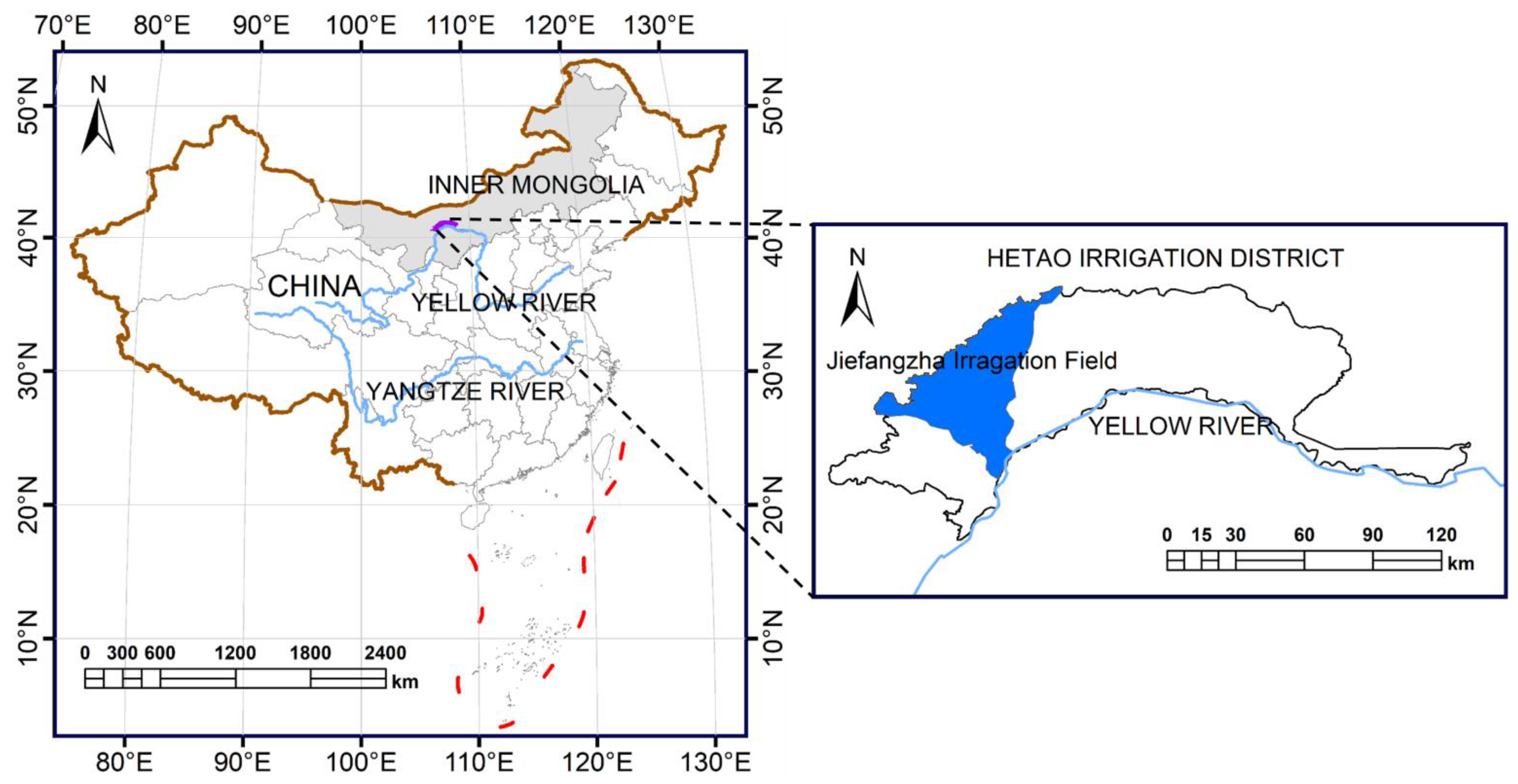
The Hetao Irrigation District (40°12′~41°20′ N, 106°10′~109°30′ E) is located in the Inner Mongolia Autonomous Region, China. It is an important grain production base and the third largest irrigation area in China. The irrigation district is divided into five major irrigation fields, namely, Ulan Buhe Irrigation Field, Jiefangzha Irrigation Field, Yongji Irrigation Field, Yichang Irrigation Field, and Wulate Irrigation Field.
The Jiefangzha Irrigation Field (40°34′~41°14′ N, 106°43′~107°27′ E), which is the second largest irrigation field in the Hetao Irrigation District, was taken as the research area (Figure 1). It is located in the west of the Hetao Irrigation District, adjacent to the Yellow River in the south, the Yinshan Mountain in the north, bordering the Ulan Buhe Desert in the west, and connected with the Yongji Irrigation Field in the east. The total area of the Jiefangzha Irrigation Field is 2345 km2, in which over 70% is farmland. It belongs to the continental arid monsoon climate of the middle temperate zone, with sufficient light, low rainfall, and a large temperature difference between day and night. The irrigation field enters the freezing stage from mid-November, and completely melts in late-May of the next year, lasting 180 days. The total water surface evaporation is 2300 mm, which is over 10 times that of the annual rainfall (151.3 mm), and the annual mean temperature is 9 °C. The food crop of the irrigation field in summer, is maize (May to October) and in spring, is wheat (April to July), and the major economic crop is sunflower (June to October), as well as a certain proportion of vegetable and fruit [14].
2.2. Data
2.2.1. In-Situ Measurement
The meteorological data used in the surface dataset consists of the daily precipitation, the daily average air temperature, the maximum air temperature and minimum air temperature, the daily average relative humidity, the daily average wind speed, and the daily sunshine duration. These data were obtained from 10 national meteorological stations distributed in or outside the Jiefangzha Irrigation Field (Table 1). The spatial interpolation used in the study was the angular distance weighting method, which can result in a relatively smooth spatial distribution. The spatial distribution of the meteorological input was thus generated from the plot-scale data collected by the meteorological stations.
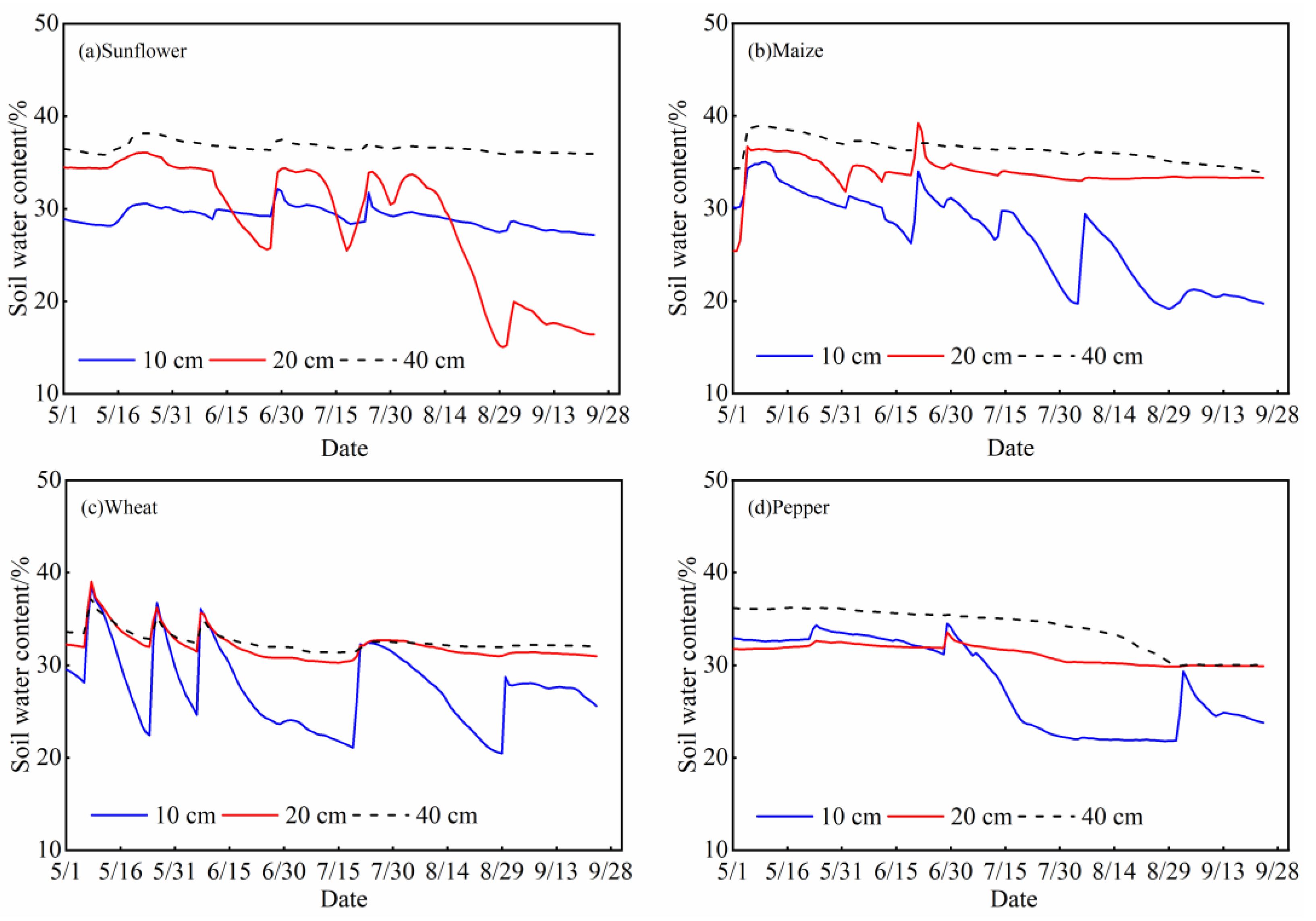
The SWC measurements were set at 10 places in the typical croplands of wheat, maize and sunflowers throughout the irrigation fields. By using the CTMS-On line system, developed by the China Institute of Water Resources and Hydropower Research, the continuous SWC and soil temperature were automatically observed and collected. The SWC profile has three sensors that reach a depth of 10 cm, 20 cm, and 40 cm, from 1 May 2014 to 24 September 2014, which covered the major growing period of the typical crops. The observation interval was one h. By eliminating the abnormal values, the daily average SWC was thus calculated from the hourly measurements (Figure 2). It shows that the moisture in the field with the sunflower cultivation is, for some time periods, lower at the depth of 20 cm, compared to the moisture at the depth of 10 cm. The sunflower has a very developed root system with a strong ability to absorb water and nutrients. It is widely and deeply distributed in the soil, and about 60% of the roots are distributed in the 0–40 cm soil layer. Most of this is at a depth about 20 cm. From mid-August to late-September, the sunflower is in the filling stage and maturity stage, and the root water absorption is high, which causes this phenomenon.
2.2.2. Remote Sensing Data
The remote sensing data used in our research were Landsat-7 ETM+ and the Moderate Resolution Imaging Spectroradiometer (MODIS) land surface product on board the Terra and Aqua satellites. Landsat-7 was launched by the National Aeronautics and Space Administration (NASA) on 15 April 1999, and carries an enhanced thematic imaging sensor (ETM+) that retains the original multispectral characteristics of the Landsat-5 thematic imaging sensor (TM). However, its spatial resolution in the thermal infrared bands is increased from 60 m to 120 m. The Landsat-7 ETM+ also adds a panchromatic bands with a spatial resolution of 15 m. In view of the advantages of the sensor in space and the spectral resolution, Landsat-7 has become one of the most commonly used remote sensing data sources, widely used in agricultural surveying, hydrological forecasting, and environmental monitoring [15]. The MOD16A2 products reflect the comprehensive effects of the global soil moisture evaporation, vegetation transpiration, vegetation canopy interception, and water evaporation, including ET, the potential evapotranspiration (ETp), the latent heat flux (LE), and the potential latent heat flux (LEp). The MODIS data provide two observations daily, at an over-passing time of approximately 10:30 am and 1:30 pm local time. Both data were re-projected into the Universal Transverse Mercator (UTM) map projection system. The images with a heavy cloud cover were removed according to the quality flags in the datasets [16].
2.3. Methodology
2.3.1. Data Fusion Method
In order to take advantage of both the finer resolution remote sensing data (Landsat-7 ETM+) and the coarse data with a shorter recurrence interval (MODIS), the ESTARFM, developed by Zhu et al. [17], was used in our research. The main idea of the ESTARFM is to make use of the correlation to blend the multi-source data and to minimize the system biases. The relationship between the coarse-resolution reflectance and the fine-resolution reflectance can be expressed as:
where F and C denote the fine-resolution reflectance and coarse-resolution reflectance, respectively; w is the search window size; t0 and tp are reference time and prediction time, respectively; (xw/2, yw/2) is a given pixel location for both the fine-resolution and the coarse resolution images; N is the size of the similar pixels, including the central prediction pixel; (xi, yi) is the location of the ith similar pixel; Wi is the weight of the ith similar pixel; Vi is the conversion coefficient of the ith similar pixel.
The final predicted fine-resolution reflectance at the prediction time tp is calculated as:
where F(xw/2, yw/2, tp, B) denotes the final predicted fine-resolution reflectance; Fm(xw/2, yw/2, tp, B) and Fn(xw/2, yw/2, tp, B) are the fine-resolution reflectance at tm and tn; Tm and Tn are the temporal weight at tm and tn, respectively.
2.3.2. ISODATA Cluster Algorithm and Spectral Matching
The Landsat-7 ETM+ images and the MODIS normalized difference vegetation index (NDVI) data were re-merged to produce a mega data tube, which was then classified using the ISODATA cluster algorithm. In the spectral matching, the algorithms need the definition of some criteria for measuring the similarity and closeness of the pixels.
The spectral similarity value (SSV) is a combined measure of the correlation similarity and the Euclidian distance, which can be formulated as:
where de is the Euclidian distance; n is the length of the NDVI time series; X and Y denote the NDVI time series; r is Pearson’s correlation coefficient, and ranges from −1 to 1.
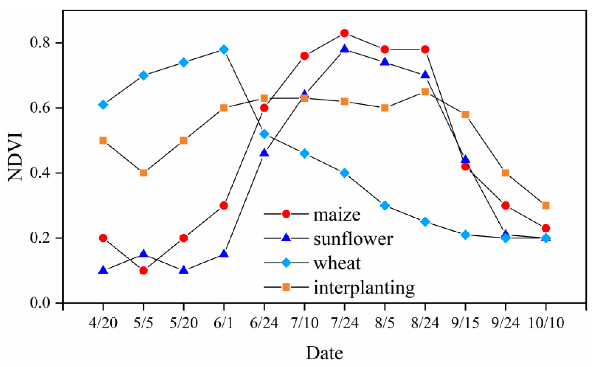
The images of the Jiefangzha Irrigation Field were divided into 50 clusters by the ISODATA algorithm, and generated the NDVI variation curve of each cluster. The statistical characteristic curves of the NDVI in the croplands were compared with the realistic NDVI curves through a survey (Figure 3), and then recognized and analyzed using the spectrum similarity.
2.3.3. SEBS Model
In 2002, Su [18] proposed a single-layer model, based on the principle of energy balance, namely the SEBS model, which has a high estimation accuracy and is widely used in drought monitoring and water resources evaluation [19]. The model assumes that the sensible heat flux of each pixel is between the dry limit and the wet limit of the pixel, which avoids the error caused by the uncertainty of the spatial interpolation of the meteorological data, to a certain extent. The SEBS model can be expressed as follows [20]:
where, Rn is the net radiation flux, W/m2; G is the soil heat flux, W/m2; H is the sensible heat flux, W/m2; is the latent heat flux, W/m2.
Rn is the difference between the total radiation from the surface up and down [21]. The calculation formula is as follows:
where, is the albedo, that is, the ratio of the flux of the solar radiation reflected from the ground to the flux of the incoming solar radiation. It is determined by the surface features and the solar altitude. Rs is the downward shortwave radiation, W/m2; is the downwelling longwave radiation, W/m2; is the upwelling longwave radiation, W/m2; is the surface emissivity.
G is the heat exchange, per unit area of soil in a unit time, and is the ratio of the heat stored in the soil and vegetation, due to conduction [21]. The empirical statistical formula is as follows:
where Ts is the land surface temperature, K; NDVI is the normalized difference vegetation index.
H refers to the turbulent heat exchange between the atmosphere and the underlying surface caused by temperature changes [21]. It is obtained from the surface temperature and the meteorological parameters, and is proportional to the temperature difference. The calculation formula can be expressed as follows:
where is the air density and its value is 1.29 kg/m3; Cp is the specific heat of air at a constant pressure and its value is 1004 J (kg · K)−1; Ta is the reference height temperature, K. is the aerodynamic resistance, m/s.
2.3.4. CWSI Method
Jackson et al. [22] proposed the crop water stress index (CWSI), based on the canopy temperature, according to the energy balance theory, formulated as:
where ETa denotes the actual evapotranspiration, which could be calculated from the MOD16A2; ETp denotes the potential evapotranspiration, which could be calculated by the Penman–Monteith method [23].
The CWSI reflects the ratio between the plant transpiration and the possible maximum evapotranspiration, which could be considered as the evaluation index of the water condition at the root layer. Under the circumstances of water stress, the ETa is the planted ET under the condition of a sufficient water supply (i.e., the ETp), multiplied by the modified soil moisture coefficient (Ks).
The Ks can be calculated by the power function method as follows [24]:
where θ is the average SWC, cm3·cm−3; θwp is the wilting water content, cm3·cm−3; θj is the field capacity, cm3·cm−3; c and d are the empirical constant, which varies from crop types and soil conditions. According to Equations (11) and (12):
The SWC could be calculated as follows:
2.3.5. Statistical Metrics
To fully evaluate the performance of the estimated SWC, three metrics were used, including the determination coefficients (R2), the mean absolute error (MAE), and the root mean square error (RMSE). The R2 indicates the fit degree of the model and the larger the R2, the better the fitting effect and the stronger robustness of the model. The RMSE indicates the prediction accuracy of the model and the smaller the RMSE, the higher the prediction accuracy of the model. The MAE is the average of the absolute value of the deviation between all individually measured values and the estimated values. Compared with the mean error, the MAE will not be offset by the positive and negative because the deviation is absolute. Therefore, the MAE can better reflect the actual situation of the predicted error and the smaller the MAE, the better the fitting effect of the model.
The metrics are calculated as follows:
where n is the number of the validation value during the day; Mi and Si are the measured and estimated SWC, respectively.
3. Results
3.1. Planting Structure
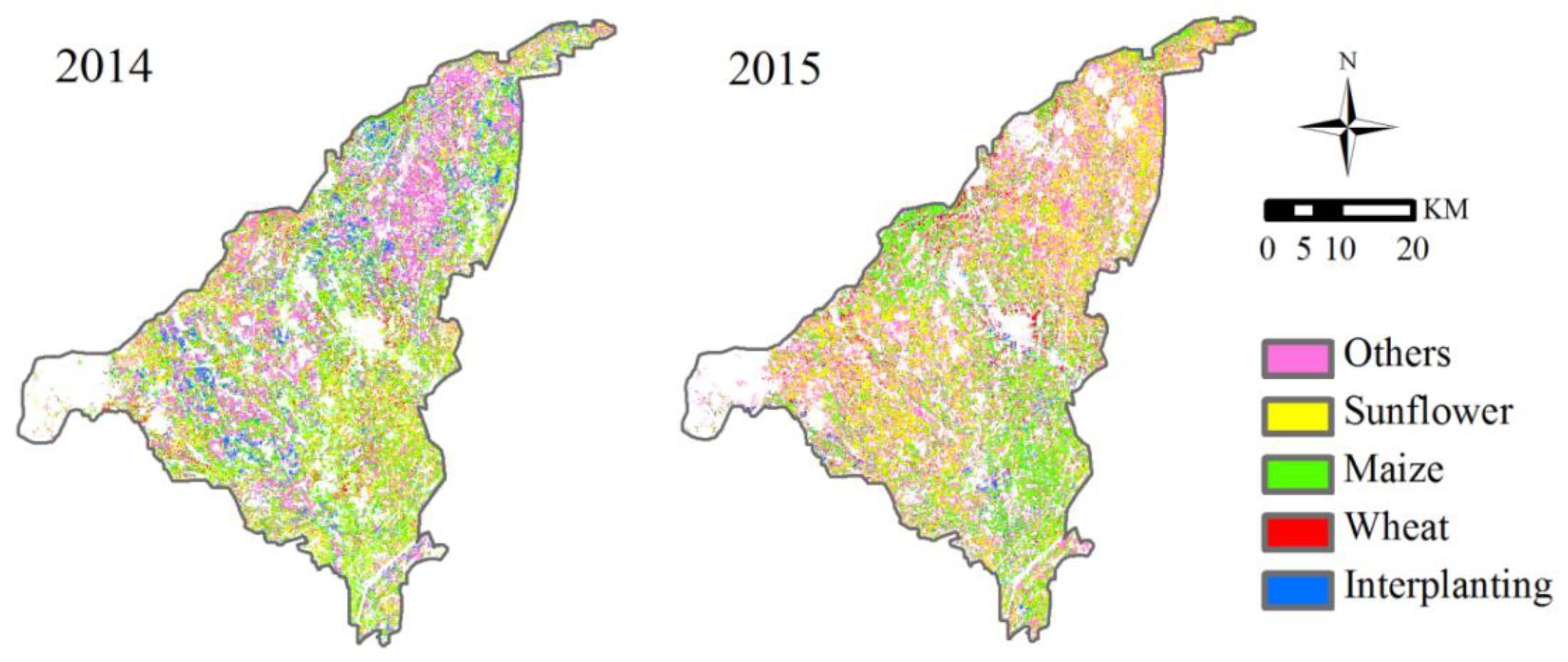
As shown in Figure 4, the crop planting structure was displayed in 2014 and 2015. The major food and economic crops are the summer maize and sunflower, respectively. The proportion of summer maize to the total cropland was 30.94% and 35.46% in 2014 and 2015, respectively, which has the largest planting area among these crops. The planting proportion of sunflower in 2014 and 2015 was 23.28% and 29.65%, respectively. The planting proportion of spring wheat decreased from 9.50% in 2014 to 5.57% in 2015. Due to the incensement of labor and the loss of the rural population, as a labor-intensive and high-yield crop type, the interplanting area decreased from 8.79% in 2014 to 3.57% in 2015. Other fruit and vegetables stay at the high proportion of 27.49% and 23.32% in 2014 and 2015, respectively.
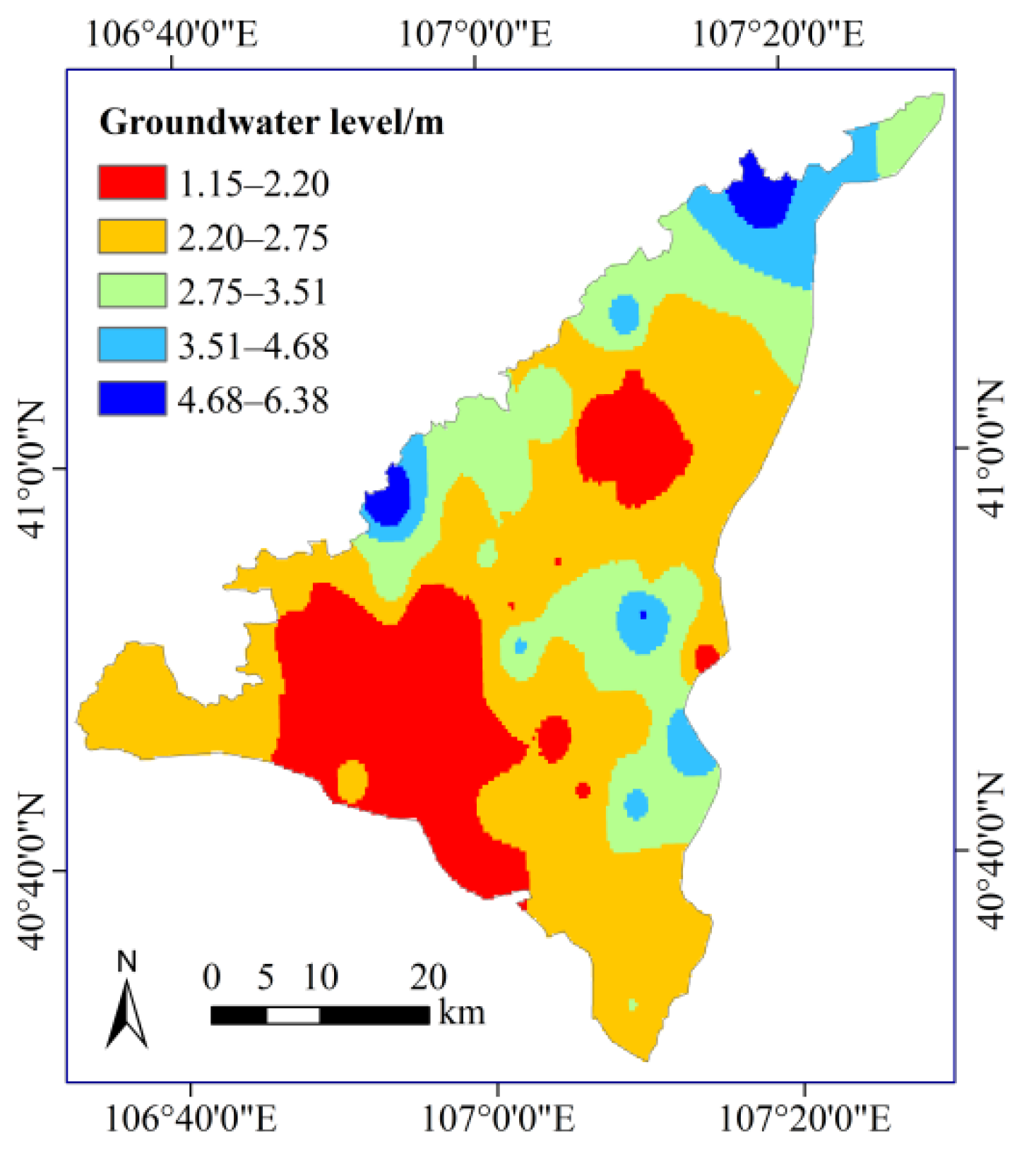
The groundwater level at the Jiefangzha Irrigation Field in March 2015, using the Kriging interpolation method [25], is shown in Figure 5. The southwest and part of the northeast areas of the study area have relatively shallower groundwater levels. Combined with the planting structure, sunflower had a higher intensity in the region with a shallower groundwater level; while wheat and maize tended to grow in the region with a deeper groundwater level, i.e., middle and southeast parts of the irrigation field. This characteristic planting structure can give suggestions for the irrigation water distribution to the management sectors.
3.2. Spatial Distribution of the ET
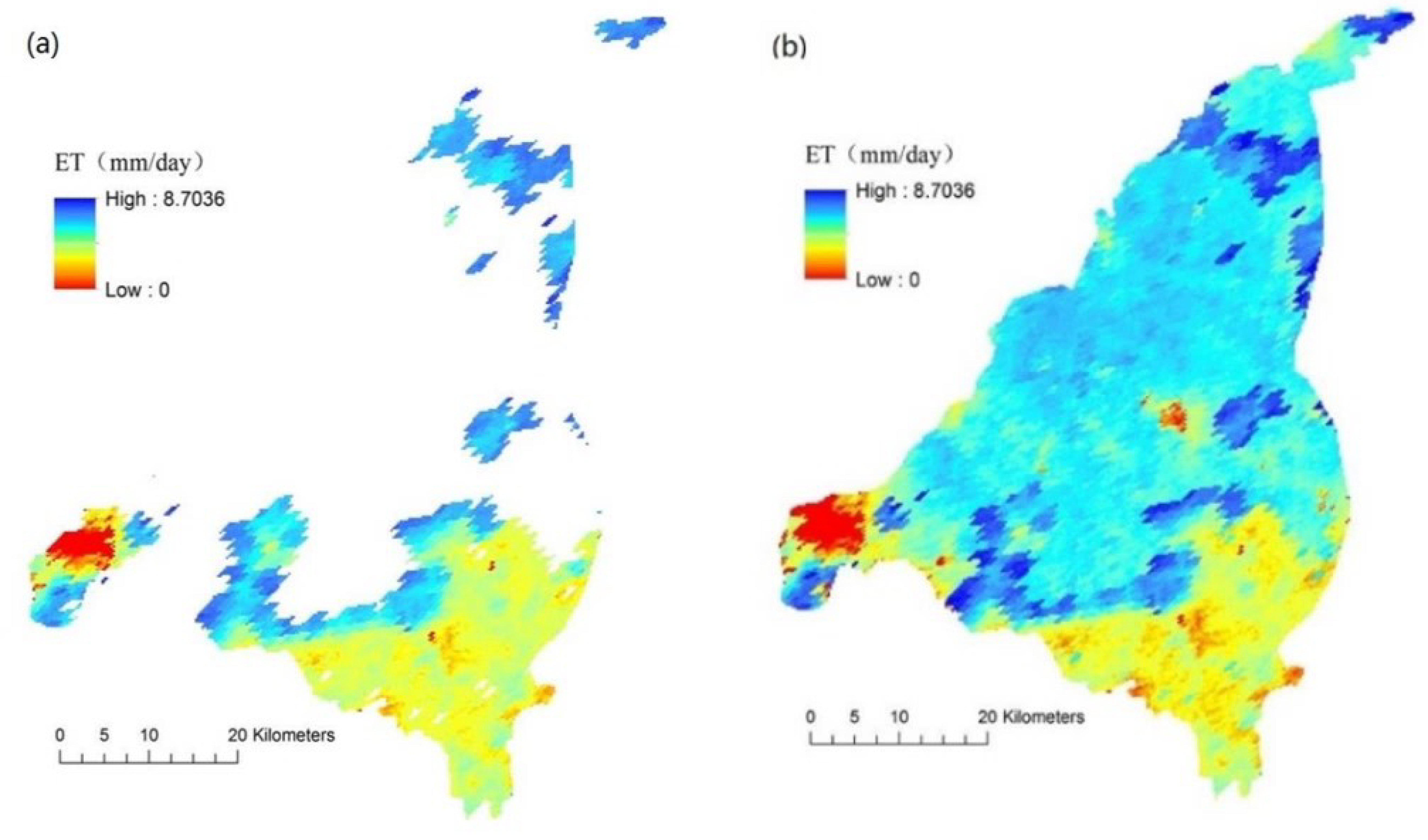
The daily ET was calculated from the MOD16A2 data on-board the Terra satellite. The results from one selected day (13 August 2014), are shown in Figure 6, in which the cloud contaminated pixels were eliminated (Figure 6a), and thus interpolated by upscaling from the continuous ET estimation from the same pixel. The Figure 6b shows that after the interpolation, the ET in the missing pixels, is smaller than the pixels exposed to clear day, which was reasonable because under the cloud contaminated pixels, the available energy (i.e., net radiation minus the soil heat flux) was smaller, due to a lack of sunshine.
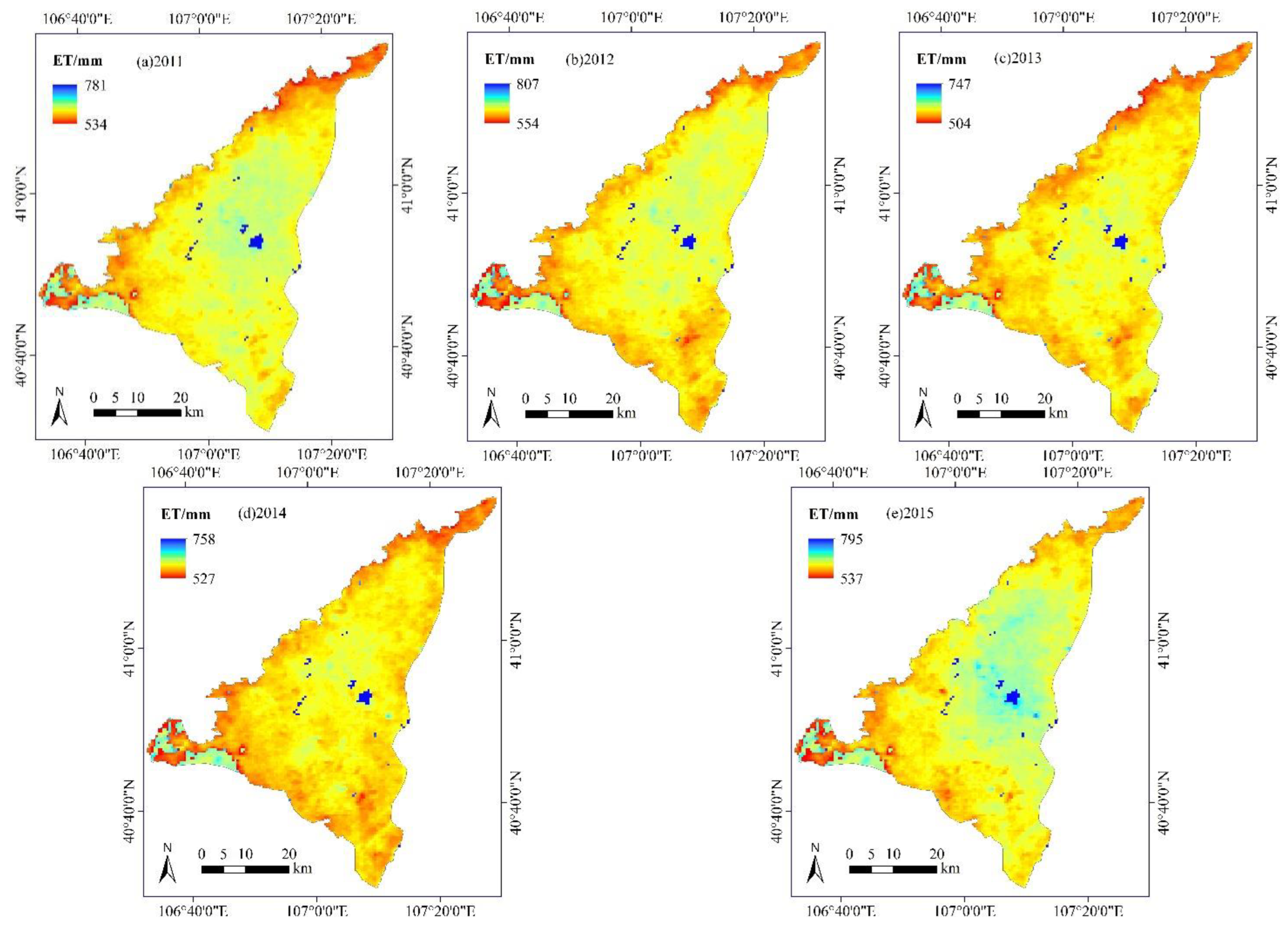
The five-year continuous regional estimation of the ET was calculated over the entire Jiefangzha Irrigation Field. Figure 7 shows the spatial distribution of the annual ET total from 2011 to 2015. The spatial mean ET, during the crop growing season (April to October) of five years over the croplands, were 530 mm, 604 mm, 563 mm, 530 mm, and 551 mm, respectively. The precipitation during the same period from 2011 to 2015, were 45.7 mm, 207.1 mm, 102.8 mm, 141.8 mm, and 111.6 mm, respectively. Despite the annual rainfall, it varied a lot in the irrigation field, due to the sufficient irrigation from the Yellow River, the ET in the study area remained at a stable level. The annual ET in 2011 was slightly lower than that in 2012, because of the severe drought in 2011, with the annual rainfall only 1/4 of that in 2012.
The spatial distribution of the annual ET in the five years, had a different pattern because of the change in the planting structure. In 2015, the ET of wheat, maize, sunflower and the interplanting during the major growing seasons (April to October) were 493 mm, 603 mm, 497 mm, and 709 mm, respectively.
3.3. Spatial Distribution of the SWC
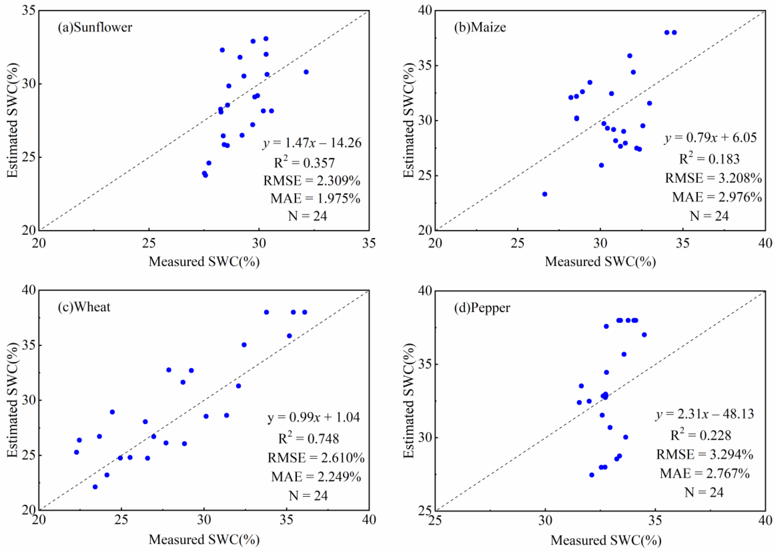
The empirical parameters c and d in Equation (15), were calculated using different crop types, including wheat, maize, sunflower, etc. Figure 8 shows the scatter plot of the estimated SWC using the remote sensing data on the clear days compared with the in-situ measurements by the CTMS-On line system at a 10 cm layer, during the growing season (April to October) in 2014. The SWC profiles measured by the CTMS-On line system were already validated by the drying and weighting method sampled twice a month near the instruments. The determination of coefficient of sunflower, maize, wheat and pepper were 0.82, 0.87, 0.73, and 0.85, respectively, which demonstrated that the SWC profiles measured by the CTMS-On line system were reliable.
The results showed that the estimated SWC, by the remote sensing data, was more discrete. Thus, some croplands tended to suffer from water scarcity, such as wheat and sunflower. Figure 8a (sunflower) illustrates a weak relationship between the measured and the estimated SWC (R2 = 0.357), and the wheat simulation results fit well with the observation. However, some sufficient irrigation croplands, such as pepper, the measured SWC was maintained at a relatively high level, therefore the remote sensing estimation not perform well.
Based on the calibration results of every single type of cropland, the spatial distribution of the SWC of the whole irrigation field, in 2014, was calculated. The planting structure distribution with a spatial resolution of 30 m is shown in Figure 4. The cropland of the Jiefangzha Irrigation Field was divided into four parts, i.e., wheat, maize, sunflower, and pepper, and then combined together.
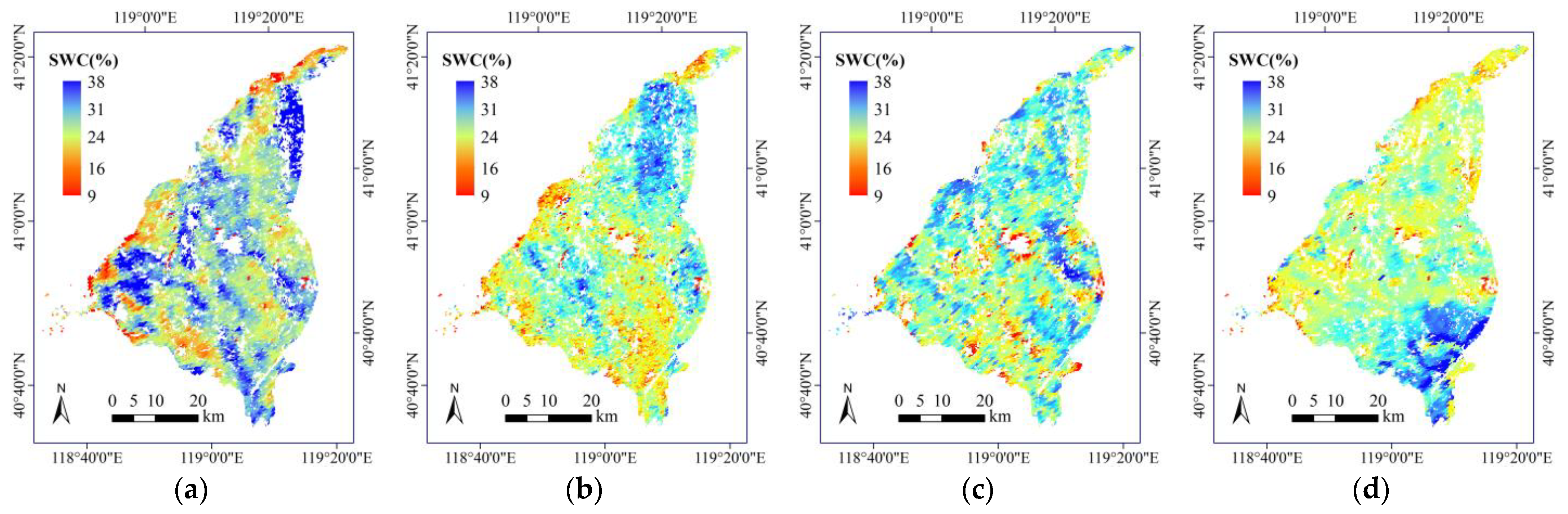
Figure 9 shows the spatial distribution of the SWC in four typical days, during the growing season, and the white pixels indicate non-cropland. The results show that at the early stage of growing season, the SWC at the surface layer is relatively small, which means that before the irrigation, during the early stage, the Jiefangzha Irrigation Field suffered, to some extent, of water scarcity. However, during July and August, the SWC of the surface layer remained at a high level because of the sufficient precipitation and irrigation.
4. Discussion
In our study, the method of the ISODATA cluster algorithm and spectral matching was used to classify the crops in the Jiefangzha Irrigation Field of the Hetao Irrigation District, and the spatial distribution of the planting structure was obtained. The ISODATA can automatically adjust the number and center of the categories in the process of clustering, so that the clustering results can be closer to the objective and the real clustering results. It is the basic data for the agricultural water resources management. According to the classification results in 2014 and 2015, the total planting area of wheat and sunflower in the field was more than 50%, which is basically consistent with the statistical data. Different from the statistical data, the planting structure extracted by remote sensing had spatial distribution information, which can provide the data support for the subsequent diagnosis of the nitrogen concentration and tracing of the non-point source pollution [26]. At the same time, we also noticed that, in addition to the classification method used in our study, many scholars have proposed several classification methods, such as the multi-source remote sensing classification [27,28,29], the object-oriented classification [30,31,32], the machine learning classification [33,34,35], and so on. These methods have been well applied in specific areas. Sun et al. [36] used the 1D-CNN machine learning classification method to identify and extract crops in the Weishan Irrigated District, Shandong Province, and achieved a satisfactory accuracy and provided good basic data for the study of the crop water consumption and agricultural water resource management. Belgiu et al. [37] used the pixel-based and object-oriented methods to map farmland in Romania with an accuracy ranging from 78.05% to 96.19%. The deficiency of our study is that there is no comparative analysis of the various classification methods, which may be a key study in the future.
The SEBS model was used to estimate the ET in the Jiefangzha Irrigation Field, from 2011 to 2015, which can provide a reference for the development of the crop irrigation systems. At present, there are many algorithms for the ET estimation. Cheng et al. [10] used the SEBAL model to produce the ET products in China, from 2001 to 2018, which provides reference for improving remote sensing algorithms. Grosso et al. [38] used Landsat-8 images to estimate the ET using the SEBAL model on a maize field in Italy and compared it with the Food and Agriculture Organization (FAO) method. The results showed that the estimated ET was in a good agreement with the ET calculated by the FAO method.
In this research, the farmland was divided into wheat, corn, sunflower, pepper, and other different underlying surfaces. The SWC of the crop growth period in the Jiefangzha Irrigation Field, from April to October 2014, was estimated. The purpose is to provide reference for the irrigation of different crops. Many scholars [7,9,39,40] have carried out remote sensing inversion of farmland soil moisture but have not classified the land features. At the same time, the validation results of the SWC in the maize farmland were not satisfactory, which may be related to the small amount of validation data (just 24). However, when some scholars [39] conducted the SWC estimation using the remote sensing method, more than 50 SWC verification points were obtained, and good verification results were obtained. Therefore, in future studies, if the conditions permit, more measured data should be collected for the model verification. Having obtained the spatial distribution information of the soil moisture, the next step would be to select the typical crops and typical farmlands in the studied region, to carry out the experimental research on the crop wilting moisture as the threshold of the lower water content. Then, the irrigation area is extracted according to the threshold value, and the irrigation water demand of each month is calculated and compared with the actual irrigation water consumption. Then, the irrigation forecast and dispatch need to be considered. The spatial resolution of the regional SWC, obtained in this study, is 250 m. This may not be enough to meet the needs of a more refined agricultural water management. However, it also has the ability to access the water demands of large regions through remote sensing. In the future, the combination of optical and microwave remote sensing can be used to obtain the daily SWC with a spatial resolution of 20 m. This can provide more valuable data for the fine management of the agricultural water resources at a regional scale.
5. Conclusions
In this research, Landsat-7 ETM+ and MODIS images were used to estimate the spatial distribution of the crop planting structure, the ET, and the SWC in the Jiefangzha Irrigation Field. The study applied the ESTAFM to generate synthetic Landsat-7 ETM+ images with MODIS and constructed the high spatial and temporal NDVI data sets. By using the ISODATA cluster algorithm, the planting structure of the Jiefangzha Irrigation Field was effectively extracted in 2014 and 2015. The positional accuracy of maize, sunflower, wheat, and interplanting are 0.81, 0.80, 0.90, and 0.82, respectively. Based on the SEBS model, the daily ET was estimated, using the long-term MODIS images. The annual ET from 2011 to 2015, well presented the spatial distribution of the ET within the study area. According to the estimated ET and CWSI, the surface layer of the SWC was calibrated and applied to the Jiefangzha Irrigation Field. The results were validated, using four in-situ measurements of the soil water profile instruments at different croplands. The validation results showed that the estimated SWC, by remote sensing on the underlying surface of wheat and sunflower, showed a good robustness, the R2 was 0.748 and 0.357, respectively, the RMSE was 2.61% and 2.309%, respectively, and the MAE was 2.249% and 1.975%, respectively. However, for maize and pepper with more irrigation times, the SWC estimation results based on the CWSI were poor, indicating that the method was more sensitive to soil drought and suitable for the crop SWC estimation with less irrigation and drought tolerance.
Author Contributions
Methodology, H.C.; Formal analysis, R.L. and H.C.; Data curation, J.C.; Validation, C.H.; Funding acquisition, Z.W.; Project administration, Z.W. All authors have read and agreed to the published version of the manuscript.
Funding
This research was funded by the National Key Research and Development Program of China (No. 2021YFB3900602), the Chinese National Science Fund (No. 52130906), the Independent Research Project of State Key Laboratory of Simulation and Regulation of Water Cycle in River Basin (No. SKL2022TS13), the Fund of China Institute of Water Resources and Hydropower Research (No. ID0145B022021, ID0145B052021), and the Fund of Hebei Water Conservancy Industry Science and Technology (No. HBAT02242202010-CG).
Institutional Review Board Statement
Not applicable.
Informed Consent Statement
Not applicable.
Data Availability Statement
Not applicable.
Acknowledgments
We would like to thank the anonymous reviewers for their long-term guidance and constructive comments.
Conflicts of Interest
The authors declare no conflict of interest.
References
- Seneviratne, S.I.; Corti, T.; Davin, E.L.; Hirschi, M.; Jaeger, E.B.; Lehner, I.; Orlowsky, B.; Teuling, A.J. Investigating soil moisture–climate interactions in a changing climate: A review. Earth Sci. Rev. 2010, 99, 125–161. [Google Scholar] [CrossRef]
- Dobriyal, P.; Qureshi, A.; Badola, R.; Hussain, S.A. A review of the methods available for estimating soil moisture and its implications for water resource management. J. Hydrol. 2012, 458–459, 110–117. [Google Scholar] [CrossRef]
- AghaKouchak, A.; Farahmand, A.; Melton, F.S.; Teixeira, J.; Anderson, M.C.; Wardlow, B.D.; Hain, C.R. Remote sensing of drought: Progress, challenges and opportunities. Rev. Geophys. 2015, 53, 452–480. [Google Scholar] [CrossRef] [Green Version]
- Robinson, D.A.; Campbell, C.S.; Hopmans, J.W.; Hornbuckle, B.K.; Jones, S.B.; Knight, R.; Ogden, F.; Selker, J.; Wendroth, O. Soil Moisture Measurement for Ecological and Hydrological Watershed-Scale Observatories: A Review. Vadose Zone J. 2008, 7, 358–389. [Google Scholar] [CrossRef] [Green Version]
- Anderson, M.C.; Norman, J.M.; Mecikalski, J.R.; Otkin, J.A.; Kustas, W.P. A climatological study of evapotranspiration and moisture stress across the continental United States based on thermal remote sensing: 2. Surface moisture climatology. J. Geophys. Res. 2007, 112, D11112. [Google Scholar] [CrossRef]
- Peng, J.; Loew, A.; Zhang, S.; Wang, J.; Niesel, J. Spatial Downscaling of Satellite Soil Moisture Data Using a Vegetation Temperature Condition Index. IEEE Trans. Geosci. Remote Sens. 2016, 54, 558–566. [Google Scholar] [CrossRef]
- Bao, Y.; Lin, L.; Wu, S.; Kwal Deng, K.A.; Petropoulos, G.P. Surface soil moisture retrievals over partially vegetated areas from the synergy of Sentinel-1 and Landsat 8 data using a modified water-cloud model. Int. J. Appl. Earth Obs. Geoinf. 2018, 72, 76–85. [Google Scholar] [CrossRef]
- Long, D.; Bai, L.; Yan, L.; Zhang, C.; Yang, W.; Lei, H.; Quan, J.; Meng, X.; Shi, C. Generation of spatially complete and daily continuous surface soil moisture of high spatial resolution. Remote Sens. Environ. 2019, 233, 111364. [Google Scholar] [CrossRef]
- Abowarda, A.S.; Bai, L.; Zhang, C.; Long, D.; Li, X.; Huang, Q.; Sun, Z. Generating surface soil moisture at 30 m spatial resolution using both data fusion and machine learning toward better water resources management at the field scale. Remote Sens. Environ. 2021, 255, 112301. [Google Scholar] [CrossRef]
- Cheng, M.; Jiao, X.; Li, B.; Yu, X.; Shao, M.; Jin, X. Long time series of daily evapotranspiration in China based on the SEBAL model and multisource images and validation. Earth Syst. Sci. Data 2021, 13, 3995–4017. [Google Scholar] [CrossRef]
- Maes, W.H.; Steppe, K. Estimating evapotranspiration and drought stress with ground-based thermal remote sensing in agriculture: A review. J. Exp. Bot. 2012, 63, 4671–4712. [Google Scholar] [CrossRef] [PubMed] [Green Version]
- Ye, N.; Walker, J.P.; Guerschman, J.; Ryu, D.; Gurney, R.J. Standing water effect on soil moisture retrieval from L-band passive microwave observations. Remote Sens. Environ. 2015, 169, 232–242. [Google Scholar] [CrossRef]
- Sadeghi, M.; Jones, S.B.; Philpot, W.D. A linear physically-based model for remote sensing of soil moisture using short wave infrared bands. Remote Sens. Environ. 2015, 164, 66–76. [Google Scholar] [CrossRef]
- Xu, X.; Huang, G.; Qu, Z.; Pereira, L.S. Assessing the groundwater dynamics and impacts of water saving in the Hetao Irrigation District, Yellow River basin. Agric. Water Manag. 2010, 98, 301–313. [Google Scholar] [CrossRef]
- Mao, K.; Qin, Z.; Shi, J.; Gong, P. A practical split-window algorithm for retrieving land-surface temperature from MODIS data. Int. J. Remote Sens. 2007, 26, 3181–3204. [Google Scholar] [CrossRef]
- Yi, Y.; Yang, D.; Huang, J.; Chen, D. Evaluation of MODIS surface reflectance products for wheat leaf area index (LAI) retrieval. Isprs J. Photogramm. Remote Sens. 2008, 63, 661–677. [Google Scholar] [CrossRef]
- Zhu, X.; Chen, J.; Gao, F.; Chen, X.; Masek, J.G. An enhanced spatial and temporal adaptive reflectance fusion model for complex heterogeneous regions. Remote Sens. Environ. 2010, 114, 2610–2623. [Google Scholar] [CrossRef]
- Su, Z.; Schmugge, T.; Kustas, W.P.; Massman, W.J. An Evaluation of Two Models for Estimation of the Roughness Height for Heat Transfer between the Land Surface and the Atmosphere. J. Appl. Meteorol. Climatol. 2001, 40, 1933–1951. [Google Scholar] [CrossRef]
- Yu, D.; Li, X.; Cao, Q.; Hao, R.; Qiao, J. Impacts of climate variability and landscape pattern change on evapotranspiration in a grassland landscape mosaic. Hydrol. Process. 2019, 34, 1035–1051. [Google Scholar] [CrossRef]
- Xue, J.; Bali, K.M.; Light, S.; Hessels, T.; Kisekka, I. Evaluation of remote sensing-based evapotranspiration models against surface renewal in almonds, tomatoes and maize. Agric. Water Manag. 2020, 238, 106228. [Google Scholar] [CrossRef]
- Yujiao, W.; Lin, Z.; Xinyu, C.; Wenke, W.; Jianshi, G.; Huilin, Y.; Dan, M. A downscaling study of evapotranspiration in Nanjing based on the ESTARFM model. Acta Ecol. Sin. 2022, 42, 6287–6297. [Google Scholar] [CrossRef]
- Jackson, R.D.; Idso, S.B.; Reginato, R.J.; Pinter, P.J., Jr. Canopy temperature as a crop water stress indicator. Water Resour. Res. 1981, 17, 1133–1138. [Google Scholar] [CrossRef]
- Zhang, F.; Liu, Z.; Zhangzhong, L.; Yu, J.; Shi, K.; Yao, L. Spatiotemporal Distribution Characteristics of Reference Evapotranspiration in Shandong Province from 1980 to 2019. Water 2020, 12, 3495. [Google Scholar] [CrossRef]
- Peng, S.; Suo, L. Water requirement model for crop under the condition of water-saving irrigation. J. Hydraul. Eng. 2004, 1, 17–21. [Google Scholar] [CrossRef]
- Judeh, T.; Bian, H.; Shahrour, I. GIS-Based Spatiotemporal Mapping of Groundwater Potability and Palatability Indices in Arid and Semi-Arid Areas. Water 2021, 13, 1323. [Google Scholar] [CrossRef]
- Han, N.; Zhang, B.; Liu, Y.; Peng, Z.; Zhou, Q.; Wei, Z. Rapid Diagnosis of Nitrogen Nutrition Status in Summer Maize over Its Life Cycle by a Multi-Index Synergy Model Using Ground Hyperspectral and UAV Multispectral Sensor Data. Atmosphere 2022, 13, 122. [Google Scholar] [CrossRef]
- Qadir, A.; Mondal, P. Synergistic Use of Radar and Optical Satellite Data for Improved Monsoon Cropland Mapping in India. Remote Sens. 2020, 12, 522. [Google Scholar] [CrossRef] [Green Version]
- Veloso, A.; Mermoz, S.; Bouvet, A.; Le Toan, T.; Planells, M.; Dejoux, J.-F.; Ceschia, E. Understanding the temporal behavior of crops using Sentinel-1 and Sentinel-2-like data for agricultural applications. Remote Sens. Environ. 2017, 199, 415–426. [Google Scholar] [CrossRef]
- Torbick, N.; Chowdhury, D.; Salas, W.; Qi, J. Monitoring Rice Agriculture across Myanmar Using Time Series Sentinel-1 Assisted by Landsat-8 and PALSAR-2. Remote Sens. 2017, 9, 119. [Google Scholar] [CrossRef] [Green Version]
- Cui, W.; Zheng, Z.; Zhou, Q.; Huang, J.; Yuan, Y. Application of a parallel spectral–spatial convolution neural network in object-oriented remote sensing land use classification. Remote Sens. Lett. 2018, 9, 334–342. [Google Scholar] [CrossRef]
- Moosavi, V.; Talebi, A.; Shirmohammadi, B. Producing a landslide inventory map using pixel-based and object-oriented approaches optimized by Taguchi method. Geomorphology 2014, 204, 646–656. [Google Scholar] [CrossRef]
- He, Y.; Franklin, S.E.; Guo, X.; Stenhouse, G.B. Object-oriented classification of multi-resolution images for the extraction of narrow linear forest disturbance. Remote Sens. Lett. 2011, 2, 147–155. [Google Scholar] [CrossRef] [Green Version]
- Barnes, M.L.; Yoder, L.; Khodaee, M. Detecting Winter Cover Crops and Crop Residues in the Midwest US Using Machine Learning Classification of Thermal and Optical Imagery. Remote Sens. 2021, 13, 1998. [Google Scholar] [CrossRef]
- Qian, S.; Hu, Q.; Zhou, Q.; Ciara, H.; Xiang, M.; Tang, H.; Wu, W. In-Season Crop Mapping with GF-1/WFV Data by Combining Object-Based Image Analysis and Random Forest. Remote Sens. 2017, 9, 1184. [Google Scholar] [CrossRef] [Green Version]
- Wang, H.; Zhao, X.; Zhang, X.; Wu, D.; Du, X. Long Time Series Land Cover Classification in China from 1982 to 2015 Based on Bi-LSTM Deep Learning. Remote Sens. 2019, 11, 1639. [Google Scholar] [CrossRef] [Green Version]
- Haoran, S.; Lei, W.; Rencai, L.; Zhen, Z.; Baozhong, Z. Mapping Plastic Greenhouses with Two-Temporal Sentinel-2 Images and 1D-CNN Deep Learning. Remote Sens. 2021, 13, 2820. [Google Scholar] [CrossRef]
- Belgiu, M.; Csillik, O. Sentinel-2 cropland mapping using pixel-based and object-based time-weighted dynamic time warping analysis. Remote Sens. Environ. 2018, 204, 509–523. [Google Scholar] [CrossRef]
- Grosso, C.; Manoli, G.; Martello, M.; Chemin, Y.; Pons, D.; Teatini, P.; Piccoli, I.; Morari, F. Mapping Maize Evapotranspiration at Field Scale Using SEBAL: A Comparison with the FAO Method and Soil-Plant Model Simulations. Remote Sens. 2018, 10, 1452. [Google Scholar] [CrossRef] [Green Version]
- Safa, B.; Mehrez, Z.; Mohammad, E.H.; Nicolas, B.; Zohra, L.-C.; Qi, G.; Pascal, F. Soil Moisture and Irrigation Mapping in A Semi-Arid Region, Based on the Synergetic Use of Sentinel-1 and Sentinel-2 Data. Remote Sens. 2018, 10, 1953. [Google Scholar] [CrossRef] [Green Version]
- Gao, Q.; Zribi, M.; Escorihuela, M.J.; Baghdadi, N. Synergetic Use of Sentinel-1 and Sentinel-2 Data for Soil Moisture Mapping at 100 m Resolution. Sensors 2017, 17, 1966. [Google Scholar] [CrossRef]
Figure 1.
The geographical position of the Jiefangzha Irrigation Field.

Figure 2.
The measured SWC in the typical croplands in the Jiefangzha Irrigation Field. (a) Sunflower; (b) Maize; (c) Wheat; (d) Pepper.
Figure 2.
The measured SWC in the typical croplands in the Jiefangzha Irrigation Field. (a) Sunflower; (b) Maize; (c) Wheat; (d) Pepper.

Figure 3.
Characteristic curves of the NDVI in the typical croplands.

Figure 4.
Spatial distribution of the main crops in 2014 and 2015.

Figure 5.
Spatial distribution of the groundwater level in March 2015.

Figure 6.
Spatial distribution of the ET on 13 August 2014. (a) before the interpolation; (b) after the interpolation.
Figure 6.
Spatial distribution of the ET on 13 August 2014. (a) before the interpolation; (b) after the interpolation.

Figure 7.
Spatial distribution of the annual ET in the Jiefangzha Irrigation Field. (a) 2011; (b) 2012; (c) 2013; (d) 2014; (e) 2015.
Figure 7.
Spatial distribution of the annual ET in the Jiefangzha Irrigation Field. (a) 2011; (b) 2012; (c) 2013; (d) 2014; (e) 2015.

Figure 8.
Scatter plot of the estimated SWC compared with the measured SWC. (a) Sunflower; (b) Maize; (c)Wheat; (d) Pepper.
Figure 8.
Scatter plot of the estimated SWC compared with the measured SWC. (a) Sunflower; (b) Maize; (c)Wheat; (d) Pepper.

Figure 9.
Spatial distribution of the SWC in the Jiefangzha Irrigation Field. (a) 4 May; (b) 9 June; (c) 18 July; (d) 23 August.
Figure 9.
Spatial distribution of the SWC in the Jiefangzha Irrigation Field. (a) 4 May; (b) 9 June; (c) 18 July; (d) 23 August.


Table 1.
Basic information about the meteorological stations.
| ID | Site Number | Longitude (°) | Latitude (°) | Elevation (m) |
|---|---|---|---|---|
| 1 | 53420 | 107.13 | 40.90 | 1056.7 |
| 2 | 53324 | 107.02 | 41.45 | 1576.8 |
| 3 | 53231 | 106.40 | 41.40 | 1509.6 |
| 4 | 53513 | 107.42 | 40.75 | 1039.3 |
| 5 | 53419 | 107.00 | 40.33 | 1055.1 |
| 6 | 53512 | 106.82 | 39.68 | 1091.6 |
| 7 | 53522 | 107.85 | 40.05 | 1184.3 |
| 8 | 53336 | 108.52 | 41.57 | 1288.2 |
| 9 | 53337 | 108.27 | 41.10 | 1022.7 |
| 10 | 53433 | 108.65 | 40.73 | 1020.4 |
Publisher’s Note: MDPI stays neutral with regard to jurisdictional claims in published maps and institutional affiliations. |
© 2022 by the authors. Licensee MDPI, Basel, Switzerland. This article is an open access article distributed under the terms and conditions of the Creative Commons Attribution (CC BY) license (https://creativecommons.org/licenses/by/4.0/).
Share and Cite
MDPI and ACS Style
Chen, H.; Wei, Z.; Lin, R.; Cai, J.; Han, C. Estimation of Evapotranspiration and Soil Water Content at a Regional Scale Using Remote Sensing Data. Water 2022, 14, 3283. https://doi.org/10.3390/w14203283
AMA Style
Chen H, Wei Z, Lin R, Cai J, Han C. Estimation of Evapotranspiration and Soil Water Content at a Regional Scale Using Remote Sensing Data. Water. 2022; 14(20):3283. https://doi.org/10.3390/w14203283
Chicago/Turabian StyleChen, He, Zheng Wei, Rencai Lin, Jiabing Cai, and Congying Han. 2022. "Estimation of Evapotranspiration and Soil Water Content at a Regional Scale Using Remote Sensing Data" Water 14, no. 20: 3283. https://doi.org/10.3390/w14203283
Note that from the first issue of 2016, this journal uses article numbers instead of page numbers. See further details here.