Water Allocation, Return Flows, and Economic Value in Water-Scarce Environments: Results from a Coupled Natural-Human System Model

Abstract

In many parts of the world including the western United States, the allocation of water is governed by complex water laws that dictate who receives water, how much they receive, and when. Because these rules are generally based on the seniority of water rights, they are not necessarily focused on maximizing economic value across the entire economy. The maximization of value from water use economy-wide is a complex optimization problem that must explicitly consider each user’s water demand, willingness to pay (WTP) function, and the feedbacks among users in a coupled natural-human system model. In this study, we distill these complexities into a simple MATLAB^® model developed to represent a two-user economy with water-dependent sectors representative of agriculture and industry. We feed the model with realistic values of relative water use, relative willingness to pay, and return flows to explore the relationships among these factors in water-limited systems. We find that the total economic value generated from water-dependent users depends primarily on the total water available in the system. However, for a given volume of water available, economic value is not necessarily maximized when all the water is appropriated to the user with the highest WTP. Rather, total economic value depends on the amount of water available, the relative WTP between the two users, and on the return flows generated from each sector’s water use. While our simple two-user model is a significant abstraction of the complexities inherent in natural systems, our study provides important insights into the coupled natural-human system dynamics of water allocation and use in water-limited environments.

1. Introduction

Across the arid western United States, water is typically allocated by some version of a prior appropriations doctrine, wherein those with the most senior water rights—typically agricultural users—receive their full allocation of water prior to any other user being able to draw from the resource (e.g., [1,2]). This “rigid” allocation of water remains in place today, even though the vast majority of recent economic growth in the West has been driven by other sectors who may have a higher value for water (e.g., [3,4,5,6]). Importantly, in many cases the initial water allocation rules did not account for return flows—water that is not fully consumed by an upstream user and is, therefore, available for downstream use—since prior appropriations rules are typically based on the volume of water withdrawn rather than the volume of water consumed (e.g., [7,8,9]). The overall result is a mismatch between water policy, allocation, and value.

Identifying a better alternative, however, requires an improved understanding of the coupled natural-human system dynamics between water allocation and return flows in river basins. 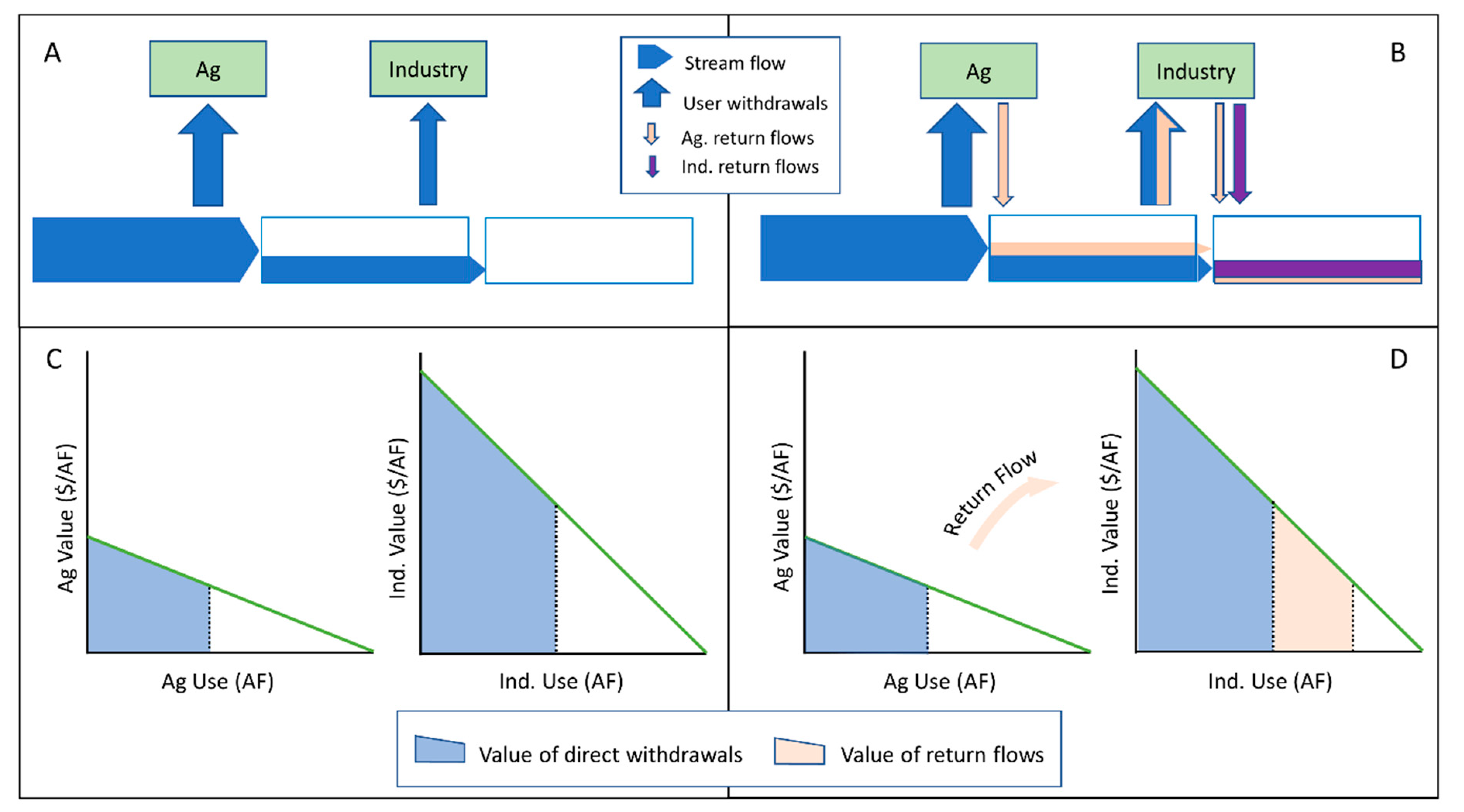Specifically, individual decisions about where and how to use water affect the volume of water available at other points in the watershed, which create feedbacks that influence the total social value the water can generate [10,11] (Figure 1). Identifying allocations that best serve society’s needs therefore requires consideration of human decision-making, the physical constraints on water availability, and the feedbacks between them.

To explore the dynamics behind this coupled natural-human system, we developed a simple model that simulates streamflow, water allocation, return flows, and economic value in an idealized basin with two water users. The users differ in the total volume of water they require, their willingness to pay (WTP) for a unit of water, and the magnitude of their return flows. Willingness to pay is shown schematically as the slope of the demand curves in Figure 1C,D, where the steeper demand curve for the “industrial” user reflects a higher value per unit of water than for the “agricultural” user. Return flows are shown schematically in Figure 1B–D, where water that flows back to the system from agricultural or industrial processes is available for downstream use and additional economic output is possible. This contrasts with a case where water allocation ignores return flows and output is limited (Figure 1A,C). We use the model to test the hypothesis that natural-human system coupling is particularly strong, and opportunities for improving water allocation efficiency are increased, when return flows are significant and when water is scarce.

Our simple model shows that total economic value depends primarily on the total water available in the system. However, for a given volume of water available, the way that water is allocated between the two users can also have a significant effect. The degree to which this allocation matters depends on both the relative WTP for water between the two users (a measure of economic value), as well as on the physical constraints on the system. These physical constraints include the relative position of each user within the basin, and the return flows generated from each sector’s water use.

We contrast the general results of these model outputs with the economic outcomes that would be expected in real systems across the arid western United States (e.g., [12,13,14]). Our model thus provides a means to evaluate the gains in economic output that could be achieved by explicitly considering both the value that each user places on water as a resource, and the return flows generated from each use. This latter component—consideration of return flows in an economic optimization framework—has often been overlooked in existing hydro-economic modeling studies, with a few notable exceptions [11,15,16,17]. This represents an important knowledge gap, since explicit consideration of return flows can significantly affect the optimal allocation of water, as described below.

2. Materials and Methods

We developed our model in the MATLAB^® computing environment. The model has a physical module and an economic module that collectively simulate water use and economic value between two water users. The physical module tracks water extraction and return flows, and provides a suite of possible water allocations that depend on the total water available, the upstream user’s water extraction, and the upstream user’s return flows. Water remaining after these extractions and return flows is available for the downstream user, who is assumed to extract as much water as available up to its maximum demand. Each of these possible allocations is then fed into the economic module, which calculates total value for each allocation based on each user’s willingness to pay curve. The model then calculates the maximum possible value for each scenario, and the water allocation that provides that maximum value.

While we abstract away from many institutional details, the two water users in the system differ in ways that are meant to capture key features of agricultural and industrial users in western basins. Specifically, production in the agricultural sector requires more water overall, and more water per dollar of output, than in the industrial sector [3,6]. However, the value of access to additional water is also generally lower for the agriculture sector than it is for the industrial sector, at the typical allocation of water determined from prior appropriations [3,4,5].

In the economic component of our model, we impose linear willingness to pay (WTP) functions to represent each sector’s marginal value per unit of water. A WTP function describes the maximum amount a user would be willing to pay to obtain an additional unit of water, as a function of that user’s total allocation of water. In the context of an agricultural or industrial user, for example, this would correspond to the user’s increase in profits due to the expanded output/sales the extra water would make possible. The maximum total economic value across users occurs at the allocation where all users have the same the WTP (see Figure 1D, where y-axis values of the last marginal unit of water for each user are equivalent). If one user has a higher WTP—for example the industrial user under prior appropriations—then total economic value can be increased by transferring a unit of water from the lower-value to the higher-value user.

The physical component of the model feeds water to the upstream user, who can extract any amount up to its maximum demand. For each possible volume extracted by the upstream user, the model calculates the resulting return flows that are then released downstream along with remaining instream flows. If each use of water in the basin were 100% consumptive (i.e., if there were no return flows), identifying the optimal allocation based on the two users’ WTP functions would be straightforward: water would simply be allocated to the higher-valued user up to its maximum allocation, or to the point where this user’s marginal WTP for the next increment of water becomes lower than the lower-valued user. However, because a change in water use upstream also affects the return flows available for downstream uses, identifying the optimal water allocation becomes significantly more complex (e.g., Figure 1B). Our contribution is to consider how changes in return flows affect the value of different water allocations, and how to maximize total value in this system.

We use the model to sequentially vary the total supply of water available, each user’s relative WTP for water, and the return flows from each sector (

Table 1. Summary of experiments designed to evaluate system response to total water, WTP ratios, and return flow fractions.

Experiment Type	Total Water (AF)	WTP Ratio	Ag Return Flow
Total Water (Section 3.1)	100	2:1	30%
	300	2:1	30%
	500	2:1	30%
WTP Ratio (Section 3.2)	300	1:1	30%
	300	2:1	30%
	300	4:1	30%
Return Flow (Section 3.3)	300	3:1	15%
	300	3:1	45%
	300	3:1	60%

). For each of these experiments, we assume that the maximum water demand from each sector is fixed. We set peak demand for the agricultural user at 500 acre feet (AF) and peak demand for the industrial user at 200 AF. We then loop through a series of allocations between users in which the upstream user takes anywhere from 0% to 100% of its total demand, subject to constraints from the total inflow. For example, if the total water available in the basin is only 300 AF, the maximum possible use by the agricultural sector is only 60% of its peak demand (300 AF/500 AF). For each of the possible water withdrawals and return flows from the upstream user, we assume that the downstream user will take as much water as remains up to its peak demand.

Our experiments result in a series of plausible water allocations between upstream and downstream users, which we combine with the WTP functions for each sector to calculate the total economic value for each scenario. We then identify the single water allocation that maximizes economic value for each scenario of total water availability, allowing us to examine how total economic value is affected by the interplay between water shortages, return flows, and willingness to pay. Finally, we compare the maximum value attainable for each scenario to the value that would be achieved under a prior appropriations allocation, in which the upstream, senior user maximizes its own output without regard to optimizing total value economy-wide.

Throughout these experiments we set actual values for agricultural and industrial uses, return flows, and other parameters for ease of interpretation. While these values were chosen to be realistic in a relative sense (i.e., total agricultural demand > industrial demand; agricultural WTP < industrial WTP) the absolute magnitudes of these parameters are less important. This is because the system dynamics are driven by the relative values of each of these parameters, as described below.

3. Results

Our analysis focused on three types of experiments: varying the total volume of water available in the system; varying the relative willingness to pay for water between the two sectors; and varying the return flows from each sector (Table 1). In the majority of these experiments, we assume that the lower-valued but higher volume user (the “agricultural” user) is upstream. Thus it is the agricultural user’s decisions, coupled with its return flows, that dictate how much water is available for the downstream, industrial user. Because the upstream user’s decisions drive water availability downstream, we also illustrate all of our results in terms of the agricultural user’s withdrawals (i.e., the x-axis for each of the figures shown below is expressed in terms of agricultural use). For clarity, we also show the remaining water available for the downstream user, which is a more complex function of the total water available, the upstream user’s withdrawals, and the upstream user’s return flows (see Figure 1).

3.1. Variation in Total Water Available

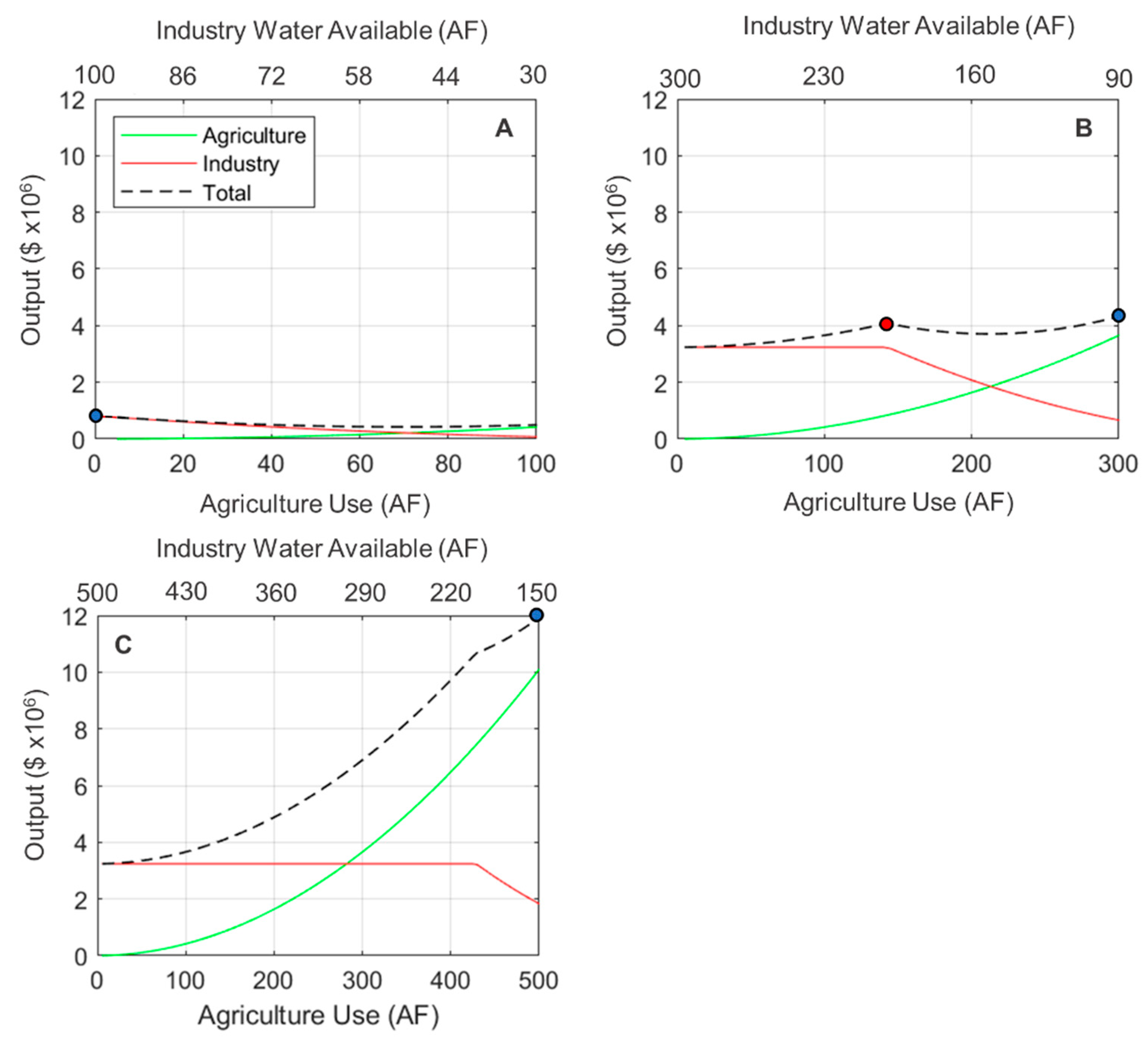
Our first set of experiments focused on varying the total volume of water available in the system. In each of these experiments, the industrial sector has a willingness to pay for water that is double that of the agricultural sector, per unit of water, and return flows from the agricultural sector are set at 30%. As expected, these experiments illustrate that economic value increases as the total volume of water increases. However, the relative allocation of water that maximizes value also varies as the total volume of water changes. This leads to a shift in water usage relative to a prior appropriations case in which the allocations are fixed.

Figure 2 illustrates this effect for three scenarios where agriculture is the upstream user, and where water is scarce relative to the total peak demand of the entire economy of 700 AF. In the scenario where water is most scarce (100 AF total), value is maximized when agriculture uses no water, and all of the water is allocated to the higher-valued industrial user downstream (Figure 2A). In a scenario with an intermediate level of scarcity (300 AF total), economic value is maximized when agriculture uses just over half of its peak demand (Figure 2B), leaving the remaining water and its return flows for the industrial user downstream. Finally, in a scenario with enough water to just meet agriculture’s peak demand, value is maximized when agriculture uses 100% of its peak demand and the industrial user relies entirely on agricultural return flows (Figure 2C).

In each of these scenarios, water is scarce relative to the total demands of the two users. However, even though industry is willing to pay twice the amount per unit of water as agriculture, the maximum value is not always achieved when this sector simply takes all the water it requires to maximize its own output. This underscores the importance of considering return flows, which can be seen in Figure 2B, where there is 300 AF of total water available. If the upstream agricultural user were to take only 150 AF of this water (red dot in Figure 2B), allowing industry to maximize its output by using the remaining 150 AF plus agricultural return flows, total economic value is actually lower than a scenario in which agriculture uses all 300 AF of the available water (60% of its peak demand; blue dot in Figure 2B). This is because the latter scenario still allows return flows to be used by the downstream industrial user, so that the total value for the industrial sector, while smaller than in the first allocation, does not go to zero.

This is also true in the scenario where there is 500 AF of total water available (Figure 2C). In this case, even when agriculture withdraws all the water from the system, its return flow (30% of 500 AF, or 150 AF) is almost enough to meet the industrial user’s peak demand as well. Thus, even though the economic output per unit of water is half as large for agriculture as it is for industry, and there is not enough water to meet the full demand of both users, total economic value is still maximized when agriculture withdraws enough water to meet its full demand, given the return flows in this scenario.

3.2. Variation in Relative Value of Water

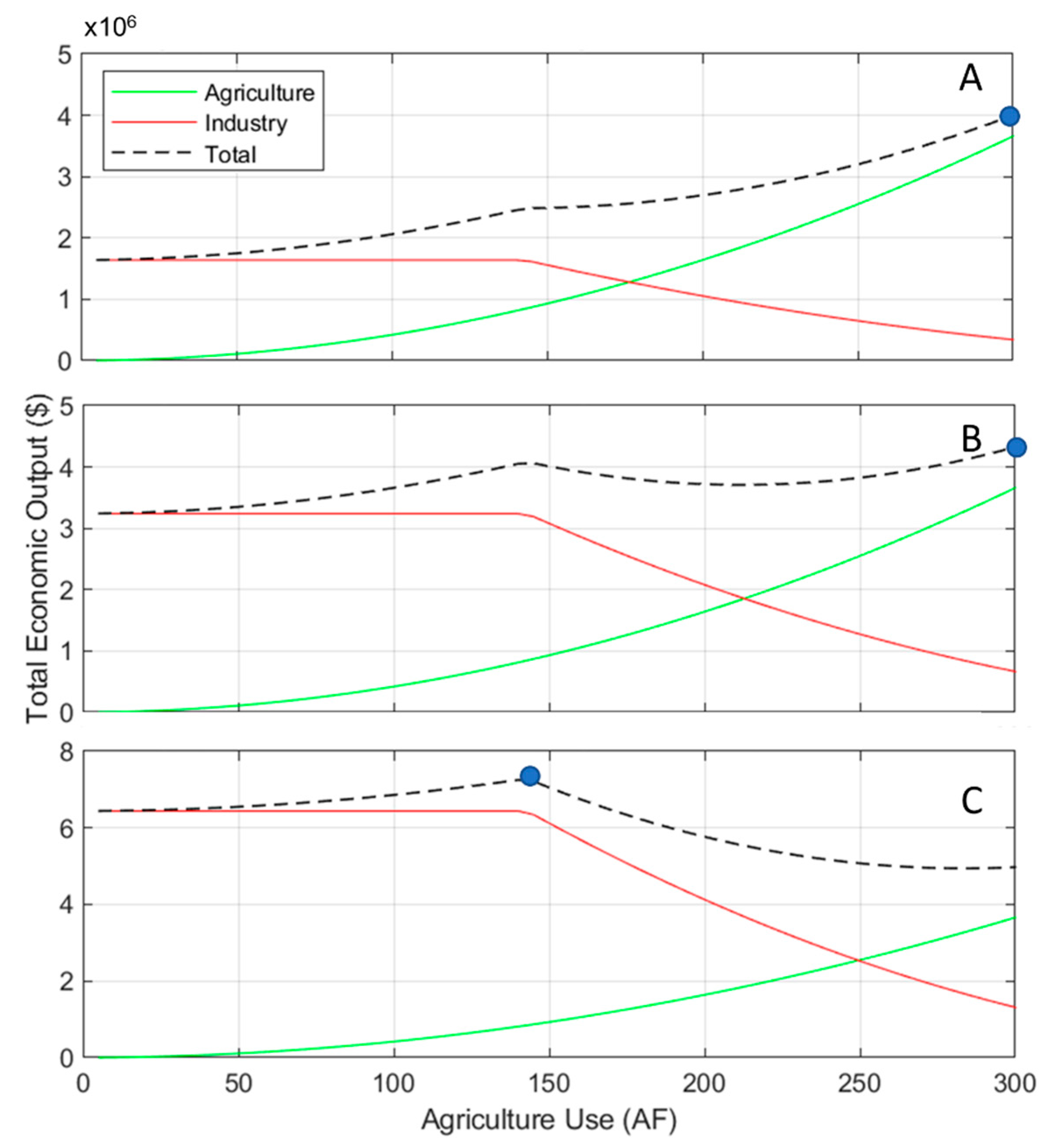
Our second set of experiments focused on understanding the relationship between the value that each sector places on water and the optimal allocation of water between the two sectors. In these experiments, we varied the relative willingness to pay for water between the two users. To do this, we varied the slope of the demand curve for the (downstream) industrial user relative to the (upstream) agricultural user and examined how the optimal allocation of water and total value changes for each of these scenarios. We characterized these differences as “willingness to pay ratios” of 1, 2, and 4, where the industrial user valued water the same, a factor of two higher, or a factor of four higher than the upstream user, per unit of water.

Figure 3A–C illustrate how the optimal allocation of water changes as the WTP ratio increases from 1 (Figure 3A) to 4 (Figure 3C), when the total water available is 300 AF (approximately 60% of the upstream agricultural user’s total demand). As shown in Figure 3, when the WTP ratio is less than or equal to 2:1, value is maximized when the agricultural sector draws all the available water and maximizes its output (blue dots in Figure 3A,B). In both scenarios, because agriculture is withdrawing its total maximum allocation, the downstream industrial user has access only to the return flow from the upstream agricultural user, which in these experiments is held fixed at 30% of agricultural withdrawals.

If the WTP ratio is increased to 4:1, economic value is maximized when the downstream industrial user is allowed to take the full 200 AF of water it requires to maximize its own output (a sum of direct streamflow plus return flows from ~150 AF of agricultural use; blue dot in Figure 3C). In this scenario, the agricultural user’s output is limited to what it can produce with only 100 AF of water, or 30% of its total demand. However, because the value of water is substantially higher for the industrial user, total value in this scenario is approximately 50% higher than the total value in either of the previous scenarios. Thus, total output is determined not only by the total water available, but also by the differences in WTP for parties at different points within the basin.

Note that in many parts of the western United States, the embedded value of water for industrial use can be orders of magnitude higher than that for agricultural use (e.g., [6]). As shown here, under realistic values of return flows and economy-wide water shortages, output is maximized when all the water is allocated to the industrial sector once the WTP ratio reaches 4:1. A re-allocation of all available water to the industrial sector would be even more heavily favored for WTP ratios higher than this value.

3.3. Variation in Return Flows

In our final set of experiments, we examined the impact on the optimal allocation of water of varying the return flow from the agricultural user’s withdrawals. As with the other parameters we explored, return flows exert the most leverage on economic outcomes when there is a water shortage. Thus, we focused these experiments on scenarios where the total water available (300 AF) is insufficient to meet the needs of both users.

Figure 4A–C illustrate how the optimal allocation of water changes as the return flows from the upstream use increase from 15% (Figure 4A) to 45% (Figure 4B) to 60% (Figure 4C). The lower return flow values of 15% and 45% broadly reflect the range of irrigation efficiencies for sprinkler and flood irrigation in agricultural systems in the Western United States, respectively [10,18]. We explore higher values of return flows primarily to evaluate how system dynamics might change with higher values. In each of these experiments, the WTP ratio is set at 3:1, representing a 3× higher value per unit of water for the downstream industrial user than for the upstream agricultural user.

The increase in return flow creates two effects, as shown in Figure 4. First, although the total volume of water available in all three of these experiments is fixed at 300 AF, the maximum economic value increases as the return flow fraction increases: the maximum attainable output with a 60% return flow is approximately 35% higher than it is when return flow is only 15%. This is simply a result of a higher total water availability for the downstream user, as return flows from the upstream user increase.

The second effect of increasing return flows is a shift in the optimal allocation of water between the upstream and downstream users. When agricultural return flows are lowest at 15%, total economic value is maximized when the agricultural sector uses only 25% of its total demand, or approximately 125 AF (Figure 4A), leaving the rest of the water for the higher-value downstream user. As agricultural return flows increase, however, the upstream agricultural sector can use a higher and higher fraction of its peak demand until at a 60% return flow it can use all the water available (300 AF, or 60% of its peak demand) while still maximizing value for the whole economy. This scenario is possible because the lost revenue due to the water shortage for the industrial sector (200 AF − 0.6 ∗ 300 AF = 20 AF shortage) is more than compensated for by the increased production from the agricultural sector upstream.

3.4. Comparison to a Prior Appropriations Scenario

For each of the evaluations above, we sought to find the allocation of water that maximized economic output, assuming that water could be freely re-allocated between users. In our final set of experiments, we compared two scenarios. The first is a “maximum value” scenario in which water can be freely traded to maximize overall economic output. The second is a “rigid” scenario in which the upstream user focuses on maximizing its own production. This latter scenario is similar to the way water is currently allocated across the Western United States: where a “senior” user makes decisions to optimize its own output, without regard to other potential water uses in the system. This system exists both because of the incentives created by the prior appropriations doctrine, and because mechanisms for water trade are currently limited (e.g., [4,14,19,20]).

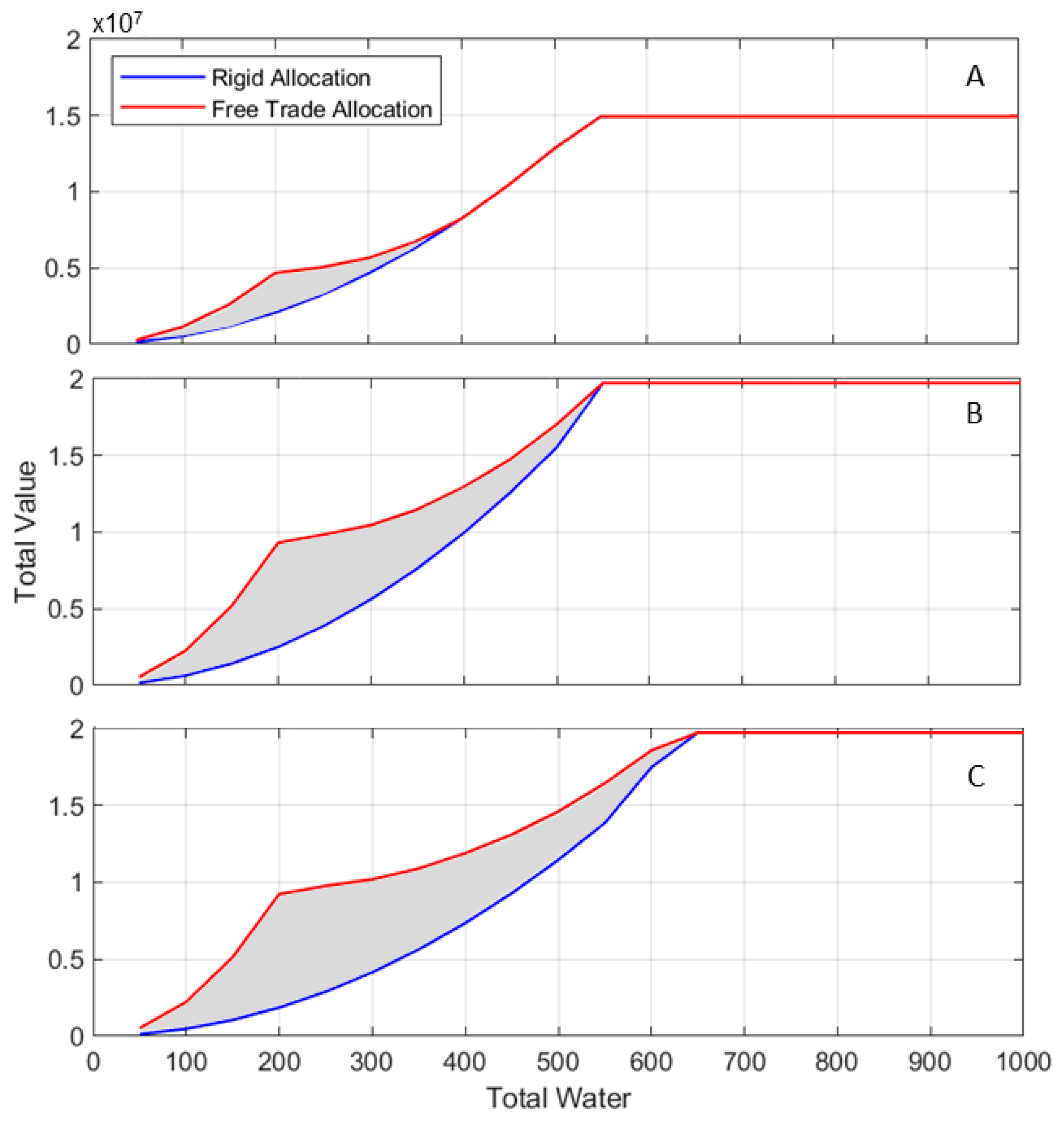
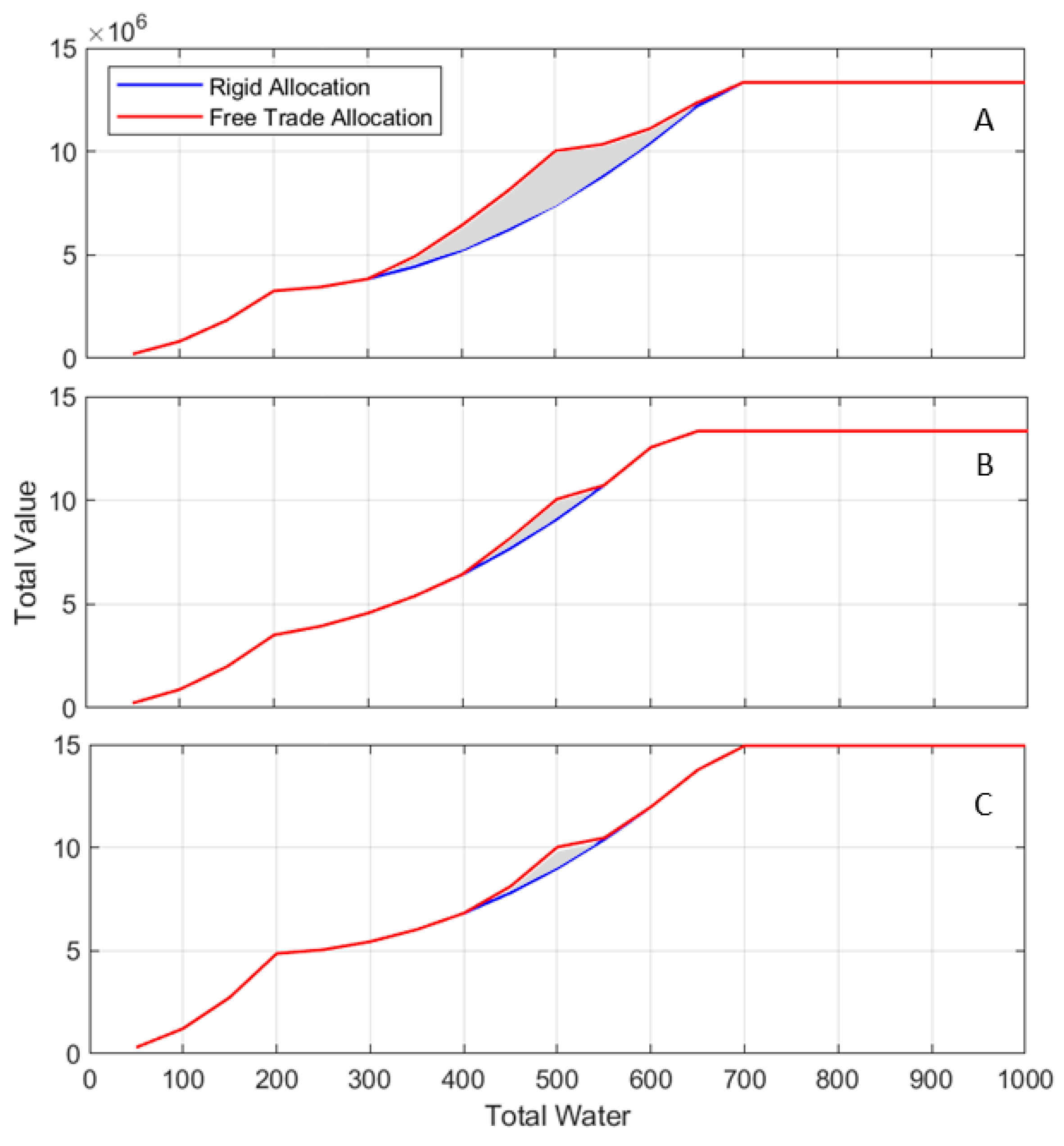
Figure 5 shows the difference in total output between these “rigid” and “maximum-value” scenarios. In all cases, the user with the lower demand but higher value per unit of water (“industry”) is downstream, and the user with the higher demand but lower value per unit of water (“agriculture”) is upstream. The blue curves (rigid) represent the attainable total value for each scenario if the upstream user focuses on maximizing its own production, and the red curve represents the maximum attainable total economic value. The benefits of re-allocation of water away from the prior appropriations regime are highest when water is scarce, as shown by the grey shaded regions highlighting the difference between the two allocations.

Figure 5A,B compare model results where the WTP ratio is 3:1 (Figure 5A) vs. 6:1 (Figure 5B). In both cases, the agricultural return flow is 30%. In each of these scenarios, the most rapid divergence between the “rigid” and “free trade” scenarios occurs between 0–200 AF of total water. Here, the added value from water re-allocation is a result of the upstream agricultural user releasing all its water to the downstream industrial user, who places a higher value on each unit of water. Beyond 200 AF, the downstream industrial user’s peak demand is fully satisfied, and agricultural production resumes. The difference between the rigid and trade optimized scenarios shrinks from this point up to a total water availability of ~400 AF (3:1 WTP ratio) or ~550 AF (6:1 WTP ratio), where the curves re-join. The location along the x-axis at which the rigid and optimized scenarios meet (400 AF vs. 550 AF) reflects the difference in optimal allocation of water between the two sectors under these different WTP ratios (see Figure 3).

Figure 5B,C compare scenarios where the agricultural return flow is 30% (Figure 5B) vs. 15% (Figure 5C) and the WTP ratio is 6:1 in both cases. As shown, the benefit of water re-allocation (grey shaded area) extends to a total water availability of ~650 AF when return flows are lower, vs. ~550 AF when return flows are higher. This is because a total water volume of 550 AF is enough to satisfy both users’ total demand (700 AF) when agricultural return flow is 30%, whereas the two users require a combined 650 AF of total water when return flows are lower.

In our initial model runs, we also modified the location of the two users in the system: placing the higher-valued industrial user upstream, rather than downstream from the lower-valued agricultural user. However, in these experiments where the higher-valued industrial user was upstream, economic value was almost always maximized when this user took its full allocation of water. The exception to this rule occurs when the WTP ratio is small and the return flow from the industrial user is also small. Figure 6 illustrates this effect for three scenarios where the industrial user is upstream. In the first two scenarios, the industrial user’s WTP is twice that of the agricultural user and its return flow ranges from 10% (Figure 6A) to 40% (Figure 6B). In the third scenario, the industrial user’s WTP is three times higher than the agricultural user and its return flow is 10% (Figure 6C).

In each of these cases, there is additional economic value to be added from water re-allocation only over a very narrow range of total water availability, if the industrial user allows all the water to be used by the agricultural user downstream. The peak increase in economic value from trade occurs at 500 AF of total water, where the complete transfer of water from industry allows the agricultural user to generate its maximum value. On either side of this peak, the range of total water availability over which trade increases economic value is sensitive to the return flow from industry and the WTP ratio. This is because the total economic value is universally higher with higher return flows or a higher WTP ratio, which limits the gains from trading downstream (compare the total value of “rigid” allocations between Figure 6A,B). The same effect occurs when the WTP ratio is higher (compare Figure 6A–C). For WTP ratios or industrial return flows much larger than the values shown in Figure 6, the advantages of water re-allocation disappear altogether.

4. Discussion and Conclusions

Our simple model demonstrates that when water is scarce relative to total demand, the total economic value from water-intensive industries can be increased when water is re-allocated relative to a “rigid” prior appropriations system. While this general result has been extensively documented in previous research on the topic (e.g., [19,21,22]), our model also illustrates several details about the dynamics of this coupled natural-human system.

Specifically, when water is re-allocated between users relative to a “rigid” allocation, we find that the change in total economic value is sensitive to at least three conditions: the scarcity of water relative to the total demand across all sectors (see Figure 2 and Figure 5); the difference in willingness to pay for water between sectors (Figure 3); and the return flows from the upstream user (Figure 4). Our model also shows that the maximum economic value for the entire economy is not always achieved when a lower-valued, upstream user sacrifices all of its output in favor of a higher-valued, downstream user. This is because a fraction of the upstream user’s withdrawals remain available to the downstream user as return flows, allowing some of the water in the system to be extracted twice. Depending on the return flow fraction from the upstream user and the relative willingness to pay for water between the two users, the downstream user may be able to maximize its value in a water-scarce scenario even if the upstream user takes a fraction of, or even all of the water for its own use (see Figure 3 and Figure 4).

Our results support the findings of previous authors who suggest that water allocations, and market mechanisms geared towards increasing economic efficiency or environmental flows, should be based on the quantities of water consumed, rather than the quantity of water extracted [9,14,17,23]. We build on the existing literature through our systematic consideration of the factors—water scarcity, relative demand and value across sectors, and size of return flows—that shape the optimal allocation in water-limited settings. While the literature has long acknowledged the failure to treat return flows as a potentially important flaw of existing water management institutions [17,24,25], our framework allows one to identify characteristics of different basins and regional economies where this flaw may be of greater or lesser significance in practice. Such an exercise is a natural first step towards rationalizing water management.

We acknowledge the legal and policy barriers that make it difficult to transition from a “rigid” allocation to a functional water market in many settings. In much of the western United States, for instance, transaction costs increase with the water transferred, as does the uncertainty of trade decisions with higher probability of opposition and appeal [19,26]. These factors serve as barriers to trade that are not considered in this simplified framework. Our economic analysis is also idealized in that we used a partial equilibrium analysis rather than a more complete, computable general equilibrium (CGE) analysis to simulate the value placed on water. Because of this, our current framework implicitly assumes that no other prices in the economy (like wages of workers in each sector) are impacted by the allocation changes described here. We further assume that there are no other market failures (tax distortions, non-market goods, etc.) that would be impacted by changes in water allocation, including environmental flows and recreational benefits. Environmental flows, in particular, could be incorporated into our modeling framework as a third “user” by monetizing these flows and expanding our optimization problem to explicitly include them [27]. This and other additional complexities are best explored in a CGE framework, which is a focus of ongoing research.

For all of these reasons, our physical model is an abstraction of real water systems, which are characterized by multiple users, externalities, and barriers to trade However, while our modeling framework is a simplification of these many complexities in real systems, it is also easily interpreted, allowing us to illustrate some of the key factors that control the dynamics of this coupled human-natural system. Future work will be focused on gradually adding complexity to the model, so that we can begin to explore time-varying water demand and supply among multiple user groups in a more realistic system.