Spatiotemporal Analysis of Groundwater Storage Changes, Controlling Factors, and Management Options over the Transboundary Indus Basin

Abstract

Intensive groundwater abstraction has augmented socio-economic development worldwide but threatens the sustainability of groundwater resources. Spatiotemporal analysis of groundwater storage changes is a prerequisite to sustainable water resource management over river basins. To estimate the groundwater storage changes/anomalies (GWCs) in the Indus River Basin (IRB), where observation wells are sparse, Gravity Recovery and Climate Experiment, the Global Land Data Assimilation System, and the WaterGAP Hydrological Model data were employed. The groundwater storage changes and controlling factors were investigated at three tier levels (TTLs), i.e., the basin, river reach, and region, to explore their implications on regional water resource management and provide management options at each level. Overall, the IRB groundwater declined from January 2003 to December 2016, with a relatively higher rate during 2003–2009 than during 2010–2016. Spatially, according to a reach-specific analysis, 24%, 14%, and 2% of the upper, middle, and lower reaches of the IRB, respectively, were indicated by a ‘severe groundwater decline’ over the entire period (i.e., 2003–2016). The GRACE-based GWCs were validated with in situ data of two heterogeneous regions, i.e., Kabul River Basin (KRB) and Lower Bari Doab Canal (LBDC). The analysis showed a correlation (R²) of 0.77 for LBDC and 0.29 for KRB. This study’s results reveal that climatic variations (increase in evapotranspiration); anthropogenic activities, i.e., pumping for irrigation; and water allocations in these regions mainly drive the groundwater storage changes across the Indus Basin.

1. Introduction

According to global estimates, approximately 43,000 km³ of renewable freshwater resources are being fed to rivers, lakes, and aquifers annually, among which 70% is consumed by agriculture, 19% by industry, and 11% by households [1,2]. Presently, 38% of the global irrigated area (i.e., 307 million hectares) is contingent on groundwater [3]. In the Indus River Basin (IRB), where canal water supplies are unreliable and insufficient, groundwater is used independently or in conjunction with surface water. As irrigation in this region is sourced mainly from groundwater [4,5], the IRB aquifer is on the brink of an alarming water crisis due to large-scale groundwater extraction [6]. Therefore, the basin’s sustainability requires proper water governance, management, and usage, especially given the complex, diversified hydrology and geopolitical nature of IRB. The key drivers of the basin’s economy are agriculture and industry. Competition among the primary users (agriculture, industry, domestic, and the environment) is spiraling as agriculture intensifies, the population grows, and people migrate to the cities [7]. Over the past several years, the continuously varying climate conditions and expansion of agricultural lands have altered the crop irrigation requirements, placing new demands on surface and groundwater resources [8,9]. Consequently, the groundwater resources in IRB have been overexploited [10].

In the Indus Basin, the overall water supply from groundwater has increased by 60% since 1960 as fresh aquifer systems are continuously pumped to meet the growing domestic and agricultural water demands [6,11]. Therefore, the groundwater aquifer system must be carefully assessed through critical long-term analysis of the groundwater storage changes (GWCs). Such an assessment builds a baseline for sustainable water use and its management. Ground-based measurement could provide a best estimate of changes in groundwater storage. However, ground-based observations are expensive and limited on spatial and temporal scales, especially in IRB, so groundwaters cannot be thoroughly monitored at different levels (regions and reaches). In particular, the limited network of observation wells reduces the understanding of the water cycle [12,13]. Policymakers and researchers believe that because there is a lack of in situ observations, groundwater regulation and the adoption of area-specific management strategies are severely compromised, especially under the effects of climate change [14]. To address these issues, many researchers are observing groundwater storage variations in real time by remote sensing observations supported by land-hydrological models at global and regional scales [5,15,16]. For example, Cheema et al. [5] employed satellite-based evapotranspiration (ET) and precipitation (P) data in the process-based Soil and Water Assessment Tool and estimated the groundwater depletion in the irrigated Indus Basin. Since the launch of the Gravity Recovery and Climate Experiment (GRACE) satellite, groundwater storage variations have been observed at different spatial and temporal scales [17] and the WaterGAP v2.2d Hydrological Model (WGHM) has emerged as a robust and qualitatively high-performing dataset of groundwater variations. The temporal changes in gravity observed by twin satellites reflect the changes in terrestrial water storage (TWS) [18]. TWS, obtained by summing the groundwater, snow water equivalent (SWE), soil moisture (SM), and surface water storage, represents the water stored above and underneath the Earth’s surface [19]. Therefore, to isolate GWCs from TWS estimated by GRACE, water storage components must be subtracted from other auxiliary datasets of hydrological models. Many researchers have already combined GRACE data with land-hydro models to study the inter-annual changes in TWS and GWCs over the Indus Basin [20,21,22] and other aquifer systems around the globe [23,24,25,26,27,28,29]. However, most of these studies analyzed TWS and GWC variations on the catchment scale; a comprehensive evaluation of GWCs over the Indus Basin is lacking at different tier levels, i.e., the basin, river reach, and region. Normally, TWS and GWC variations are mainly caused by the combined effect of climate variability and human interventions [30]. Climatic parameters, i.e., precipitation (P), runoff (R), evapotranspiration (ET), and glacier recession, are influential factors of the changes in TWS and GWC [31]. Anthropogenic activities, i.e., groundwater abstraction, land use, and irrigation, also impact TWS and GWCs in populated areas [32]. Hence, it is important to investigate GWC and its controlling factors in IRB to ensure sustainable development of the basin as a whole. The water management in IRB is administered under the Indus Water Treaty 1960 at the international level [33], and administrative regulations are implemented province-wide under the Water Apportionment Accord 1991 at the national level [34]. Therefore, in addition to basin-scale studies, it is imperative to investigate the spatiotemporal dynamics of groundwater and its controlling factors at the regional (provincial) level to provide management options for each management unit. Due to the heterogeneity that exists among different reaches of IRB in terms of topography, land use, climate and agroecological conditions, and surface water distribution quotas, IRB was divided into three reaches (i.e., upper, middle, and lower). Due to these heterogeneities, there is considerable variability in the socio-economic conditions of the above-mentioned reaches. Therefore, hypothetically, human and natural controlling factors do vary among these reaches. In this regard, it is imperative to examine the groundwater changes both in space and time at the reach level in IRB.

Considering the limitations of previous studies in the Indus Basin [5,17,20,21,35,36,37,38,39], the novelty being captured in this study includes the following: (i) investigation of the groundwater dynamics at three tier levels (TTLs), i.e., the basin, river reach, and region, using GRACE and GLDAS for the period 2003–2016 to explore their implications on regional water resources management; (ii) assessment of the controlling factors (climatic and anthropogenic) at three tier levels to mitigate the vulnerability of groundwater resources; and (iii) identification of the hotspots of groundwater change patterns by decomposing and analyzing time series of the GRACE-extracted GWC, the Potential Groundwater Use (PGWUSE), and the Potential Groundwater Withdrawal (PGWWW) to explore groundwater management options.

2. Materials and Methods

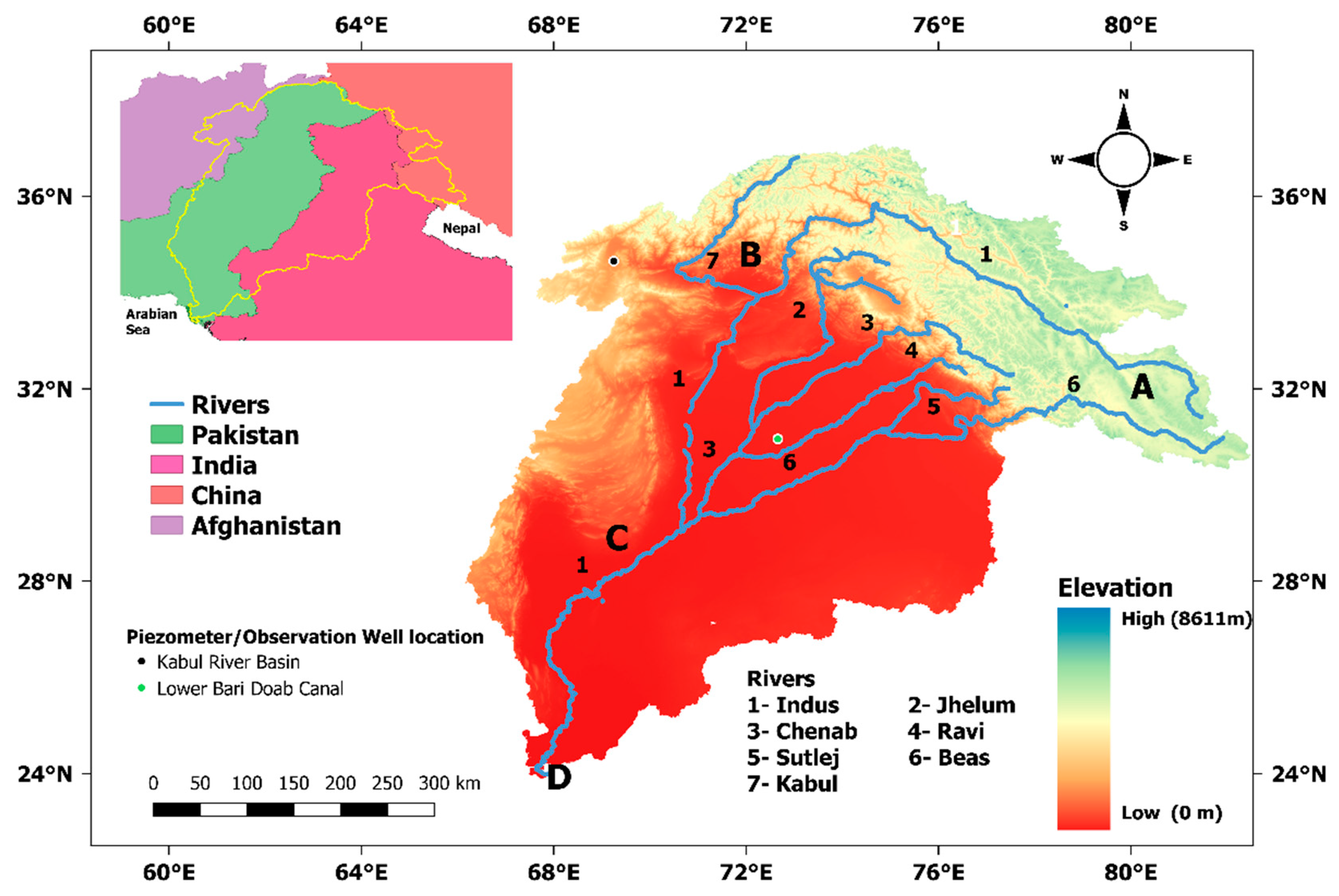
2.1. Study Area

The area coverage of IRB is approximately 1.12 million km². It is shared among Pakistan (47%) and India (39%), followed by China (8%) and Afghanistan (6%) [2] and is situated between 66.3–82.47° E longitude and 24.63–37.05° N latitude (Figure 1). The Indus River (approximately 3000 km long) originates in the Tibetan Plateau near Mount Kailash (altitude 5500 m) and traverses towards the Arabian Sea [40]. The tributaries of IRB are the Indus, Jhelum, Chenab, Ravi, Sutlej, and Bias Rivers. The eastward-flowing tributary is the Chitral River, which originates in Pakistan, flows towards Afghanistan, and then drains into the Indus River in Pakistan [41]. The basin’s climate ranges from subtropical arid and semiarid to temperate sub-humid on the plains of the Sindh and Punjab provinces to alpine in the northern mountainous highlands [2]. The average annual precipitation varies from 100 to 500 mm in the lowlands to approximately 2000 mm in the mountainous ranges. Moreover, the snowfall at higher altitudes (>2500 m) accounts for a significant part of the river flows in IRB. Although the higher peaks in the Upper Indus Basin (UIB) restrict the intrusion of monsoons, the low-lying areas in the northwest of the basin are subjected to monsoon rainfall, influencing GWCs over the basin.

IRB is divided into upper, middle, and lower reaches based on its topography and climate. The upper reach includes Kashmir, Gilgit Baltistan, and Himachal Pradesh, which constitute the major watershed of IRB (points A to B). The middle reach (points B to C) comprises the major portions of Pakistani Punjab and Indian Punjab (the food basket of Pakistan and India), which produces most agricultural products and secures the region’s food supply. The lowest part of the reach consists of Sindh (points C to Arabian sea), as shown in Figure 1. Agricultural production is influenced by waterlogged and saline agricultural lands in Sindh and some portions of Baluchistan.

Geologically, IRB is dominated by thick quaternary sediments. These sediments are mainly alluvial and deltaic deposits of fine- to medium-grained silt, sand, and clay. Coarser sands and gravels are present on the plain’s upland margins while sand deposits can be found at the east of the Indus Plain (i.e., Thar and Cholistan). Cenozoic and Mesozoic sedimentary rocks can be found in a north–south region located at the west of the Indus Plain, which stretches from Peshawar to Karachi. Older sediments (Paleozoic) and crystalline base rocks (e.g., granites and metamorphic) are mainly found in the north, including Khyber Pakhtunkhwa, Jammu and Kashmir, and Gilgit regions. Groundwater yields from these sediments are typically in the range of 50–300 m³/h down to a depth of 150 m.

2.2. Data Sources

We extracted the monthly TWS data of GRACE RL-06 released by the National Aeronautics and Space Administration (NASA) from 2003 to 2016, covering the globe with a spatial resolution of 1° × 1°. The GRACE landmass datasets of three laboratories, namely, the Centre for Space Research (CSR), Jet Propulsion Laboratory (JPL), and Geo Forschungs Zentrum Potsdam (GFZ), were obtained from the NASA website (www.jpl.nasa.gov accessed on 17 December 2019) supported by the NASA MEASUREs Programme [42,43,44,45]. The gridded surface-mass anomalies were derived from GRACE mission measurements and estimated the Earth’s mean gravity at the specified time. For the JPL datasets, scaling factors were applied to convert the 3-degree gaussian filter resolution to 1-degree spherical harmonics solutions. These grids represent the storage of the terrestrial water cycle and ice magnitudes over the entire land. Furthermore, the non-captured atmospheric and oceanic processes are included in the corresponding GRACE component. The SM, SWE, and canopy water storage (CWS) were collected from GLDAS_NOAH10_M_001 at a 1° × 1° spatial resolution [46]. The data from WGHM by the Institut für Physische Geographie, University of Frankfurt, accurately simulates the changes in all forms of terrestrial water storage and GWC except glaciers [47] to observe the agreement with GRACE-based GWC. The outputs of this model have been widely used in recent years [31,48]. The present study used the recent GWC, PGWUSE, and PGWWW data collected from 2003 to 2016, with a monthly temporal resolution and a spatial resolution of 0.5° × 0.5° [47]. To explore the controlling factors of TWS and GWC, we extracted the data of three hydrological fluxes (P, ET, and runoff (R)) from different sources. The precipitation data of the Tropical Rainfall Measuring Mission (TRMM, version TRMM-3B43 Level-3) with a temporal resolution of 1 month and a spatial resolution of 0.25° × 0.25° were obtained from NASA [49]. The monthly ET, P, and R data, output of WGHM with a spatial resolution of 0.5° × 0.5°, were taken from data published on the Earth and environmental science website [47].

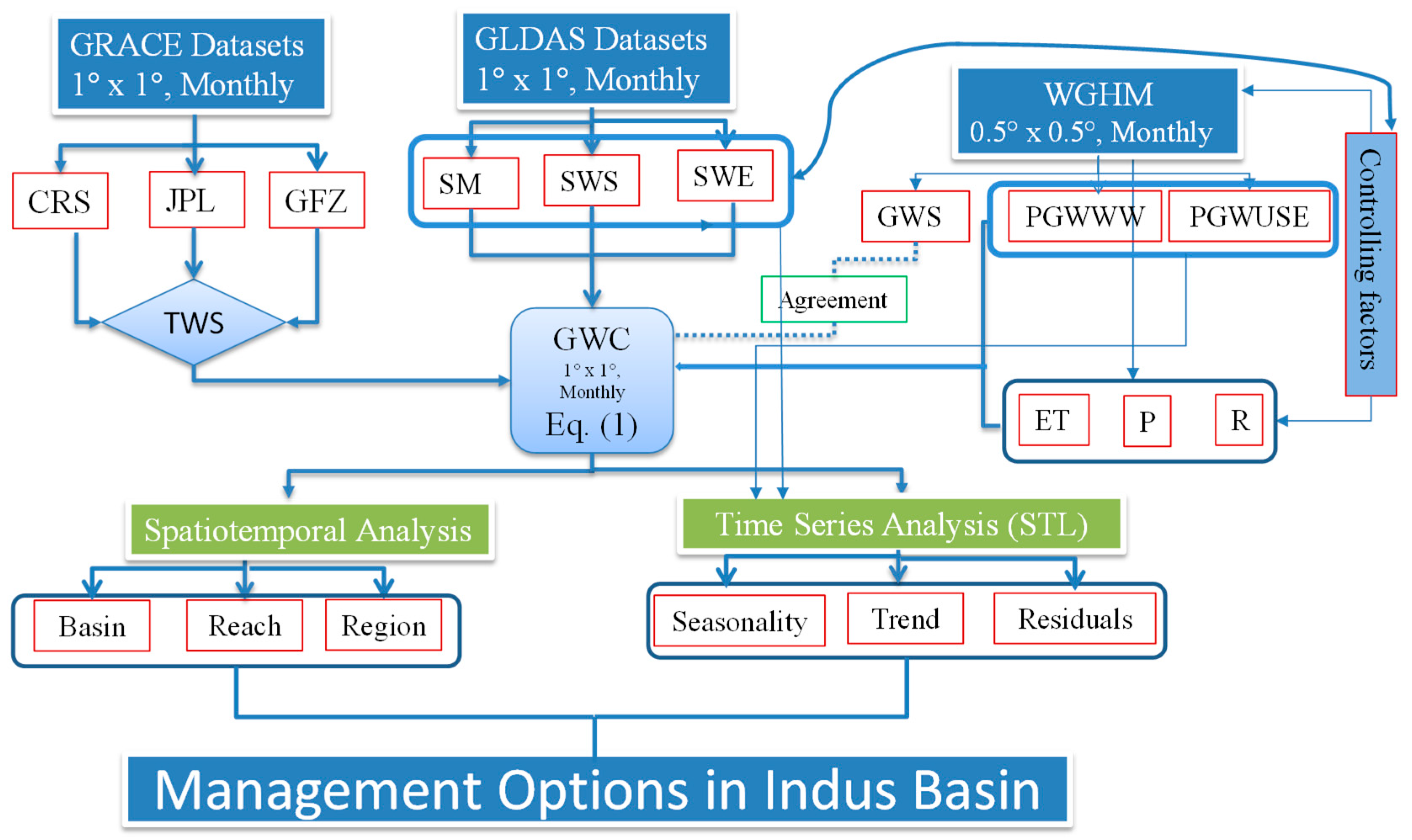
2.3. Methods

The TWS data of IRB was obtained from the three laboratories using a specialized program written in R and averaged to compute GWC. To calculate the monthly GWC, SM, SWE, and SWS were excluded from the average gridded TWS values of the JPL, CSR, and GFZ laboratories. The groundwater storage change/groundwater anomaly $\Delta GWC$ was calculated as given in Equation (1) [50,51]:

$$\Delta GWC=TWS-\Delta SM-\Delta SWE-\Delta CWS$$

(1)

where $\Delta SM$, $\Delta SWE$, and $\Delta CWS$ are the anomalies for soil moisture, snow water equivalent, and total canopy water, respectively. All variables in Equation (1) (downloaded on a rectangular grid) were imported into a geographic information system (GIS) to mask the irregular boundaries of the Indus River Basin. The centroids of the rectangular grids were obtained as the grid coordinates, and the variables of Equation (1) extracted by the R-code quantified the spatiotemporal groundwater dynamics at various levels. The TWS values for missing months were determined by a linear interpolation technique [52], and statistical analyses were performed by Mann–Kendall tests, regression, and Spearman’s rho correlation.

2.3.1. Time-Series Decomposition

A filtering procedure that decomposes a time series into its seasonal (S), trend (T), and residual (R) components using locally weighted scatterplot smoothing is commonly known as the STL method [53]. Numerous hydrological studies [54,55] have used STL to clarify, refine, and obtain the detailed characteristics of variations in timing data. STL decomposition based on LOESS at the time i in a time series Yi is given as:

$$Yi=Si+Ti+Ri \mathrm{where} i=\left(1,2,3\dots ,N\right).$$

(2)

In this study, the time series of GRACE-based GWC, PGWUSE, and PGWWW were decomposed, and the characteristics of each decomposed component were analyzed to extract valuable information. Figure 2 summarizes the datasets and research methodology as a flowchart.

2.3.2. Spatial and Temporal Analysis

Spatiotemporal analysis was performed to understand the groundwater dynamics of the basin using the available datasets. The 112 grids of the GRACE and GLDAS datasets covering the entire IRB were extracted using the GIS tool. The GRACE-based groundwater anomaly was averaged from January 2003 to December 2016 in each grid cell in the spatial analysis. The temporally averaged GWC values were then categorized into five classes based on GWC threshold values, providing more direct information for groundwater resource management options and planning [12]. The groundwater thresholds were identified by observing the range of GWC values over the IRB grids. The anomaly categorization is given in

Table 1. Groundwater change categories in the Indus River Basin.

Sr. No	Groundwater Changes (mm)	Indication of Groundwater Change
1	<−100	Severe decline
2	−100 to −50	Minor decline
3	−50 to 0	Normal variation
4	0 to 50	Minor rise
5	>50	Abnormal rise

.

2.4. Performance Assessment of the Groundwater Storage Changes

GWCs estimated in this study across the wider IRB were evaluated at two random pixels both at the very extreme northwestern part (KRB) and at the downstream LBDC. The piezometric data of KRB was obtained from Taher et al. [56], which are monthly records and available for a period of 2005–2013 while for that of LBDC’s, there are only two records available per year (i.e., pre and post monsoon) available from 2003 to 2015. The observation wells’ data for LBDC was obtained from the Punjab Irrigation Department (Pakistan).

3. Results

The estimated spatial and temporal changes in GWC revealed a groundwater decline over the study period. The fluctuations in GWC were higher before 2010 compared to the later period (2010–2016), i.e., reflecting a substantial decrease in the GRACE-based groundwater storage anomaly in the earlier period (Figure 3a,c).

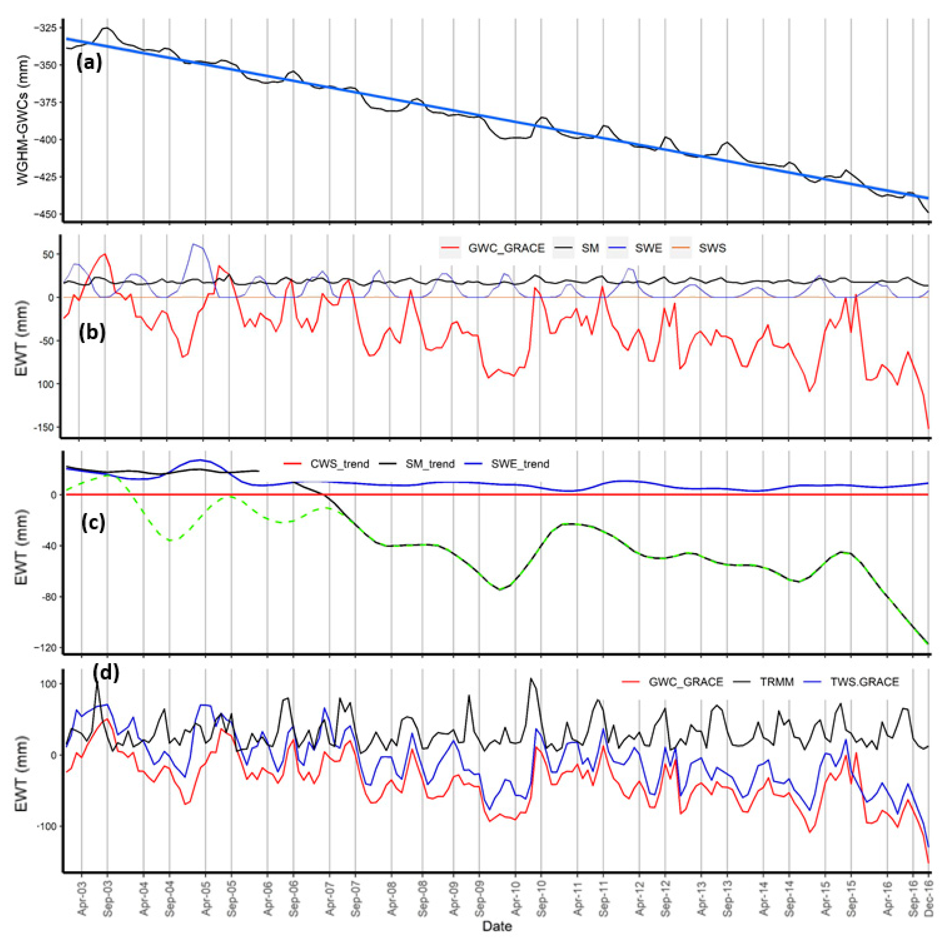
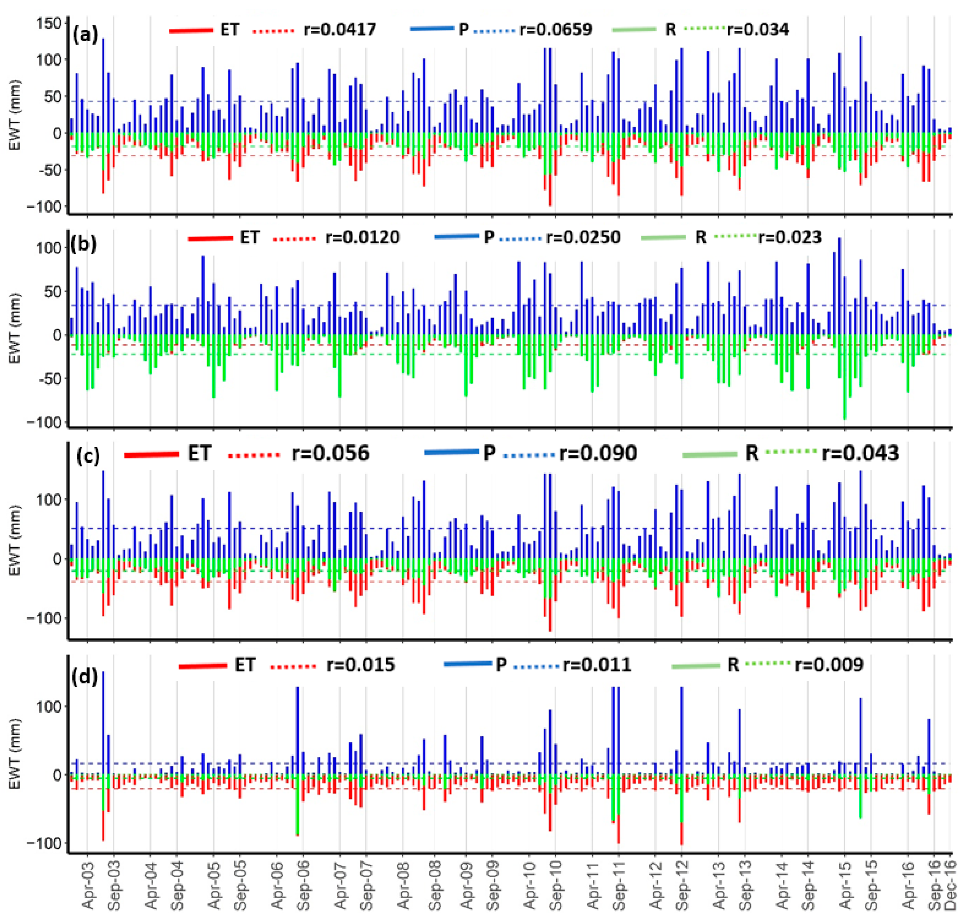
3.1. Spatiotemporal Groundwater Dynamics and Controlling Factors at the Basin Level

Figure 3a shows the temporal changes in the groundwater resources at the basin level. During the study period (January 2003 to December 2016), GWC decreased (p = 2.2 × 10⁻¹⁶; t-test) over the entire IRB. The mean GWC was −25.67 mm for the period of January 2003–December 2009 and −54.33 mm for January 2010–December 2016 (red lines in Figure 3a), confirming both a decline and shift in the mean GWC over the study period, and the fitted regression line (blue line in Figure 3a) showed an overall decreasing trend of 0.44 mm per month.

For the whole study period 2003–2016, the GWC trend declined at −0.44 mm/month in the GRACE model and −0.64 mm/month in WGHM. To identify the hotspots and understand the characteristics of GWC, the GRACE-based GWC time series was decomposed to observe its seasonality, trend, and abnormalities (see Figure 3). Across the entire IRB, the decomposed GWC signal showed a strong seasonality, with annual losses in the pre-monsoon period (around April) and annual gains in the post-monsoon period (around September) (Figure 3a,b). In each year, the seasonality curve dipped after April (Figure 3b) as excessive pumping for rice cultivation began. No significant changes were observed within the years in the seasonal component. The decomposed trend component (Figure 3c) of the GWC signal significantly declined until the end of the drought year (2009). Accordingly, groundwater changes (Figure 3c) were steeper in the first half of the study period, indicating an alarming decline in groundwater resources during this period as evident from the Mann–Kendall trend analysis, which indicated that the mean GWC was highly significant during the study period from January 2003 to December 2009 (p = 1.65 × 10⁻⁷) compared to January 2010–December 2016 (p = 1.99 × 10⁻⁴).

The groundwater level maximally declined in 2009, when the weak monsoon created drought conditions in the basin before the flood years [57]. Subsequently, it rose in the flood years, indicating the changes in groundwater mainly depend on the trend component. The residual component (a powerful indicator of abnormalities such as flood and drought events in the region) displayed abnormal signals in the winters of 2012 and 2015 (Figure 3d). In the Federal Flood Commission report [58], the years 2010–2016 were identified as flood years. Indeed, the groundwater levels showed a significant rise during these years, indicated by a wet period (Figure 3a) in the present analysis.

The spatial analysis revealed an overall decrease in groundwater resources throughout the basin. As shown in Figure 4, GWC declined from south to north and from west to east. A strip of severe GWCs was observed in Gilgit Baltistan, Kashmir, Himachal Pradesh, and Indian Punjab. In UIB, GWCs dominated in the range from −131 to −81 mm, indicating high groundwater storage variations with higher standard deviations. In the southwest part of IRB, the groundwater storages are minimum and with low variance. In general, the regions where the standard deviation of groundwater storage was high showed greater groundwater decline.

Groundwater storage changes were further explored using the SM, SWS, and SWE data from the GLDAS Noah model. Groundwater changes showed a declining trend in the study area (Figure 5a), and SWS contributed little to GWCs and their tendency (Figure 5b,c). The snow changes remained around zero because snow and ice concentrate in the mountainous part of the basin (upper IRB) and only cover parts of the Indus Basin. The SWE, which significantly affected the changes in groundwater storage, trended downward, particularly after 2005 (Figure 5c). The main contributor to GWC was SM, which is necessary for the growth and survival of flora. The occurrence of drought depends on when the current soil moisture cannot meet the plant’s requirements. As shown in Figure 5c, SM and GWC exhibited the same declining trend patterns after the winter of 2007, indicating that GWC and SM are heavily dependent on each other in IRB.

The spatial differences in TWS and GWC were analyzed from the variabilities in ET, P, and R. We mainly analyzed the entire IRB, UIB, Middle Indus Basin (MIB), and Lower Indus Basin (LIB). In the Indus Basin, TWS and GWC declined at a rate of −0.545 and −0.640 mm/month, respectively; and ET, P, and R varied by a rate of 0.0417, 0.0659, and 0.034 mm/month, respectively (Figure 6a). The positive variability rates of ET, P, and R indicated that all these variables were sensitive to TWS and GWC. However, R is generated by precipitation and snowmelt in the study area, and contributed a minor amount to TWS and GWCs. Thus, we inferred that the ET increase was the main controlling factor of the groundwater and total water storage dynamics across IRB during the study period.

In UIB, TWS trended upward at an amount of 0.018 mm/month, whereas GWC declined at an amount of 0.22 mm/month. Both P and R showed a positive tendency with higher variability than ET (Figure 6b). P increased at an amount of 0.025 mm/month, whereas ET increased at an amount of 0.012 mm/month, indicating that the P increase mainly caused the TWS increase. The increasing trend of regional R was not consistent with the P variation (Figure 6b), suggesting that there is an additive water supply from snowmelt and glacier recession. Muhammad et al. [59] reported a negative mass balance in upper IRB, with the most negative values ranging from −0.34 ± 0.31 to 0.44 ± 0.27 m w.e., with −1 in the Jhelum, Chenab, and Ravi sub-basins of the Himalaya. SWE in UIB changed by −1.02 mm/year (the glacier area was 115,675 km² in 2016). Therefore, our analysis suggests that glacier recession (not ET) is an important controlling factor of TWS and GWC variations in UIB.

In MIB, TWS and GWC significantly declined at an amount of −0.89 and −0.9604 mm/month, respectively. P and ET showed a positive tendency over time and higher variations in MIB than in the Indus Basin as a whole (Figure 6c). The rising ET trend accounts for most of the TWS loss. Meanwhile, the increasing trend in regional R (Figure 6c) is consistent with the P variation. Therefore, ET, groundwater usages and withdrawal were inferred to be the main factors that increase the TWS deficit and reduce the groundwater in MIB.

In LIB, TWS increased at a rate of 0.17 mm/month, whereas GWC declined at a rate of −0.138 mm/month. The variations in P, R, and ET were small and inconsistent with the TWS changes (Figure 6d), suggesting that precipitation and evapotranspiration are not the main factors leading to changes in the total water storage and GWC in this region. Instead, the surface water supply in terms of high water allowances to the canals provided by the Water Apportionment Accord (WAA) 1991 might explain the small groundwater and total water storage changes. The century-old irrigation system of IRB has allowed a variable allocation of surface water by its design [60]. The provincial bodies reviewed surface water allocations (WAs) at many stages to establish water rights and distribute the water of IRB among the four provinces of Pakistan, and these reviews led to a mutual consensus policy document: the Water Apportionment Accord (WAA) 1991 [60].

Precipitation markedly affects the spatial pattern of TWS and GWC and accelerates the spatial variation signal in the north–south direction. Figure 5d compares the mean monthly precipitation data from TRMM and the mean monthly TWS and GWC. The precipitation generated by TRMM varied from 2.28 (October 2007) to 107 mm/month (July 2010), whereas GWC ranged from −152.43 (December 2016) to 50.46 mm (September 2003).

As shown in

Table 2. Correlations between TRMM precipitation, TWS, and GWC.

Correlations
Spearmen’s Rho		TRMM	TWS	GWC	SM
	TRMM	1.000	0.214 *	0.188 *	0.743 *
	TWS	0.214 *	1.000	0.907 *	0.299 *
	GWC	0.188 *	0.907 *	1.000	0.241 *
	SM	0.743 *	0.299 *	0.241 *	1.000

* Correlation is significant at the 0.01 level (two-tailed).

, the TRMM, TWS, GWC, and SM data were positively correlated, indicating that the GWC values are affected not only by precipitation but also by parameters associated with anthropogenic activities, such as pumping. As shown in Figure 7a,b, the groundwater use in each year was lowest in February and highest in October. The PGWUSE started to increase after April as the rising temperature accelerated ET and rice cultivation activities in the basin. The decomposed trend components of PGWUSE and PGWWW showed highly reciprocal correlations with the trend of GWC (when PGWUSE was maximum, GWC was minimum; see Figure 7c). The monthly potential total water withdrawals from the groundwater resources were highly seasonal, minimal in April, and highest in November each year (Figure 7d,e). These results imply that much of the groundwater is withdrawn during cropping seasons and consumptive use. The trend component of the decomposed time series of PGWWW increased as the area became more dependent on groundwater (Figure 7f).

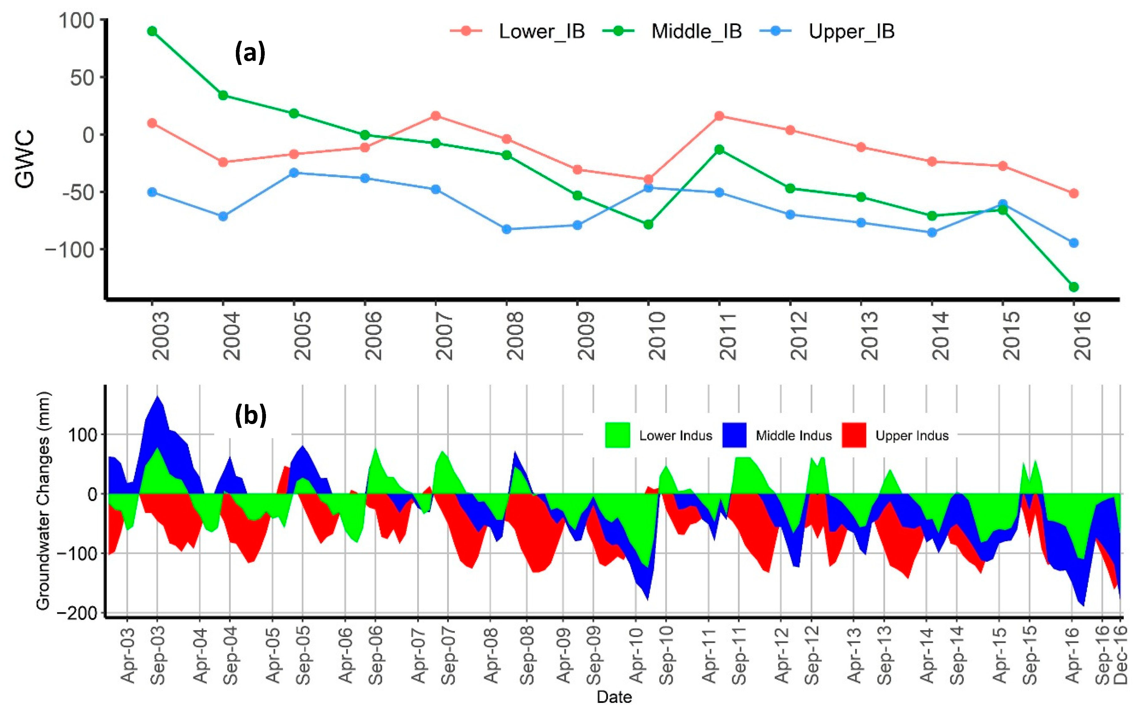
3.2. Spatiotemporal Groundwater Dynamics in Different Reaches

Reach-wise groundwater storage analysis revealed that changes in groundwater storage were diverse among the three reaches of IRB (Figure 8a) during the study period. The lower reach showed relatively higher groundwater storage than the middle reach while GWC in the upper reach was much smaller than in the middle reach (Figure 8a). These differences can be explained by variations in ET, R, P, and groundwater withdrawals as described above. GWCs in the upper and middle reaches declined more rapidly in later years than in previous years. Moreover, after 2009, GWC was higher in the middle reach than in the other reaches. Contrarily, GWC as determined for each of the reaches showed monotonous behavior during the study period. In the lower reach, the minor increases during 2007 and 2011 were contributed by groundwater recharge from flooding periods in previous years, explaining the smaller declining trend than the other reaches (Figure 8a).

Looking at the monthly scale groundwater changes (Figure 8b), we found no consistency in groundwater storage fluctuations among the three reaches during 2003–2009. However, the upper and lower reaches showed some consistency in their fluctuations during 2010–2016 (Figure 8b). In the upper reach, groundwater storage remained low in winter (~December) throughout the study period except for rising trends during the summer of 2005–2007 and 2010. The groundwater storage changes remained high during 2003–2008, and low in the rest of the study periods. The lower reach depicted high groundwater storage in the summer (~September). After the year 2009 (tipping year), groundwater storage values were continuously negative in the upper and middle reaches, indicating that the groundwater storage continuously remained lower when compared with the base period (2004–2009). Prior to 2010, all the reaches showed groundwater storage fluctuation in the range of −150–150 mm. After 2010, there was a less declining trend of the groundwater storage due to floods, and the annual minimum values were recorded during the study duration.

The most recent study year (2016) showed severe signs of depletion in groundwater storage, especially in the middle reach, as shown in Figure 9b. The upper reach showed surprisingly strong groundwater declines (<−100 mm) in all years except 2006, whereas the middle reach showed strong declines in groundwater storage from 2010 to 2016 onwards (Figure 9a,b). In general, the upper reach had the highest number of months that experienced severe groundwater declines compared with the other reaches during the study duration (Figure 9d). At the same time, there were no months with an abnormal rise (>50 mm) in the upper reach. The reach-specific analysis revealed that more rapid fluctuations in the upper reach make its ecosystem vulnerable, which may require further attention. Groundwater depletion in the upper reach should be mitigated with climate mitigation strategies.

In the reach-specific analysis, 24%, 14%, and 2% of the time span of the groundwaters in the upper, middle, and lower reaches, respectively, were severely depleted over the entire period. These findings indicate the vulnerability of groundwater resources in the upper Indus reach (Figure 9d). During the same period, GWC rose abnormally in the middle reach. The reach-wise analysis revealed more rapid fluctuations in the upper reach, which may require further attention. In particular, groundwater depletion in the upper reach should be mitigated with climate mitigation strategies.

3.3. Spatiotemporal Groundwater Dynamics at the Regional Level

To study GWCs in a spatially explicit way, the study area was subdivided into eight regions: Kashmir and Gilgit Baltistan, Tibet–China, Khyber Pakhtunkhwa, Afghanistan, Punjab, Sindh, Baluchistan, and Indian Punjab–Himachal Pradesh–Haryana (hereafter referred to as the Indian part), along the Indus River from upstream to downstream. All eight regions of IRB exhibited irregular annual patterns of continuous decline in GWC after 2003 (Figure 10). China, Afghanistan, KP, and Sindh showed consistent groundwater storage changes within the range from 0 to −50 mm except in 2016. Before 2009, groundwater changes were within −50–100 mm for all the regions while after 2010, all the regions showed a rise in groundwater storage in 2011 and then a continuous decline. In the Indian part, the groundwater storage declined until 2010, but in the years beyond 2010, GWCs were in the range of −150 mm. The low GWC values in the Tibet–China and Indian part of IRB in the second phase and particularly in the final year of the study period (2016) indicate a severe groundwater decline in these regions (see Figure 10). In the province of Sindh, the groundwater rose abnormally in 2011 and, after that, continuously declined at a lesser rate than in the other regions.

The GRACE-based estimates of groundwater storage changes were compared to in situ measurements (1 piezometer data for KRB and 1 observation well for LBDC). In situ measurements for KRB and LBDC were available from 2003 to 2015 and 2005 to 2013, respectively. When the GWC and in situ measurements were compared, the correlation coefficients for LBDC and KRB were 0.78 and 0.35, respectively (Figure 11).

4. Discussion

Overall, our analysis revealed that regional GWCs in time and space could be derived from remote sensing data (GRACE) and data assimilation models (GLDAS). In the temporal analysis, a significant decline in GWC (p = 2.2 × 10⁻¹⁶) was observed over the entire study period (January 2003 to December 2016). The observed decreasing trend and fluctuations were larger before 2010 than in the second half of the study period, which is driven by the higher values in 2003 and very low numbers in 2010. The second phase of the time series is characterized by lower levels and extreme lower levels of GWC in 2016.

In the spatial analysis, a significantly declining trend in GWC was observed in the upper Indus reach, indicating a dominant snow receding effect [61]. On the regional scale, the aquifer storage showed a declining trend in upper Punjab (especially in Gujranwala, Sialkot, and Hafizabad) because the pumping rate was high in these regions. Similar results were reported by Qureshi et al. [62], Shoaib et al. [37], Arshad et al. [39], and Iqbal et al. [20], who mentioned that water is over-pumped at an alarming rate in areas where high delta crops (i.e., rice) are grown at a high tube well density. The groundwater depletion was moderate in the districts (Faisalabad, Vehari, Pakpattan, and Khanewal) of Pakistani Punjab because groundwater is overexploited to meet the crop water requirements (Iqbal et al. (2017)). Qureshi [63] reported that groundwater is declining to below 6 m in more than 50% of the irrigated area of Punjab, causing groundwater quality deterioration and increased pumping costs.

Groundwater storage changes were severe in the Indian part of IRB, reaching a maximum in 2016. Dominant changes in groundwater were observed in the south-eastern regions of the IRB, covering Himachal Pradesh, Indian Punjab, Haryana, and Rajasthan (the northern Indian states, which account for 95% of groundwater use in the region). High groundwater-based irrigation can explain these large changes, which has expanded to meet the wheat and rice demands of Indian government policy [64]. Other causes of groundwater decline are exponential population growth and rapid economic development [65], which have increased the pumping of groundwater [5,66], in addition to the provision of subsidies on electricity and diesel for groundwater abstraction, an increased number and density of tube wells (>30/km² in different districts), augmented groundwater draft, expansion of rice and wheat areas [39], and spikes in cropping intensity [67,68]. Similarly, Rodell et al. [17] detected a significant groundwater depletion in the north-western part of India based on the GRACE datasets. They calculated a mean depletion rate of 40 ± 10 mm/year equivalent height of water, whereas Asoka et al. [69] estimated a 20 mm/year groundwater decline rate in the same region. Singh and Bhakar [70] reflected upon the alarming groundwater situation in Rajasthan and concluded that there is an uncertain future for this commodity. Steenbergen et al. [71] attributed groundwater exhaustion in the Baluchistan province of Pakistan to the intensive use of water for agricultural purposes. The Sindh province of Pakistan, the southwest part of IRB, showed lower GWC fluctuations than the other parts of the basin and similar results were revealed by Arshad et al. [39]. Basharat and Azhar [60] attributed the lower GWCs to the higher water allowance of canals under WAA 1991. Therefore, the authority responsible for the WAA 1991 should rationalize water allowances over IRB to counteract waterlogging and salinity in the lower reach (i.e., the Sindh province of Pakistan) and over-abstraction of groundwater in the upper part of the basin. The observed in situ groundwater anomalies were compared with the estimated GRACE-based groundwater storage anomalies (Figure 11). The results were consistent with the study conducted by Akhtar et al. [38] and Ali et al. [37].

Due to drought conditions, the groundwater declined maximally in 2009 while during flood periods, groundwater storages were improved. Chen et al. [18] reported in Songhua River Basin that flood and drought conditions characterize the fluctuation in groundwater storage. GWS recovery was attributed to an increase in precipitation [72] in the Tasmania region, Australia, after 2010. However, Indus Basin exhibited a decline in groundwater storage that was inconsistent with the precipitation variation till 2010 (Figure 5c). Afterwards, it showed a continuous decline due to the significant impact of anthropogenic activities, i.e., mainly pumping in agriculture (Figure 7c,f). In addition, Feng et al. [73] also reported that the pumping of groundwater for irrigation and coal mining activities was a major contributing factor in North China.

The spatiotemporal patterns of groundwater behavior extracted from the GLDAS and GRACE data might assist the implementation of sustainable groundwater management by policymakers and managers. Admittedly, the spatial resolution of the GRACE mission is too coarse to monitor the finer surface mass changes in large water bodies such as dams and lakes. Although the applied datasets are the best current data sources for determining GWCs in this area, they are insufficient for understanding groundwaters in canal command areas. Moreover, the mission ended in 2017, necessitating a new perspective of groundwater dynamics. To this end, statistical modeling of the GRACE time series and downscaling of GRACE to the local scale of groundwater dynamics are required. By connecting the data of GRACE, the latest launched GRACE-FO, and statistical modeling, we can ensure the continuity of the groundwater dynamics for prediction, especially when data are missing during the operation period of GRACE-FO. Issues such as sea water intrusion, how surface water bodies affect groundwater quality and quality, and land subsidence are not addressed by GRACE [74]. The uncertainties in hydrological models, i.e., GRACE and GLDAS, could be considered in the perspective studies.

5. Conclusions

The GRACE and GLDAS datasets were combined into a novel algorithm that estimates the spatial and temporal changes in groundwater, thereby providing water-resource management options at the basin, reach, and regional levels. Groundwater resources in the whole basin have declined over time but exhibited a spatially heterogeneous change pattern. The main conclusions of this study and outlooks for future research and policy intervention are summarized as follows:

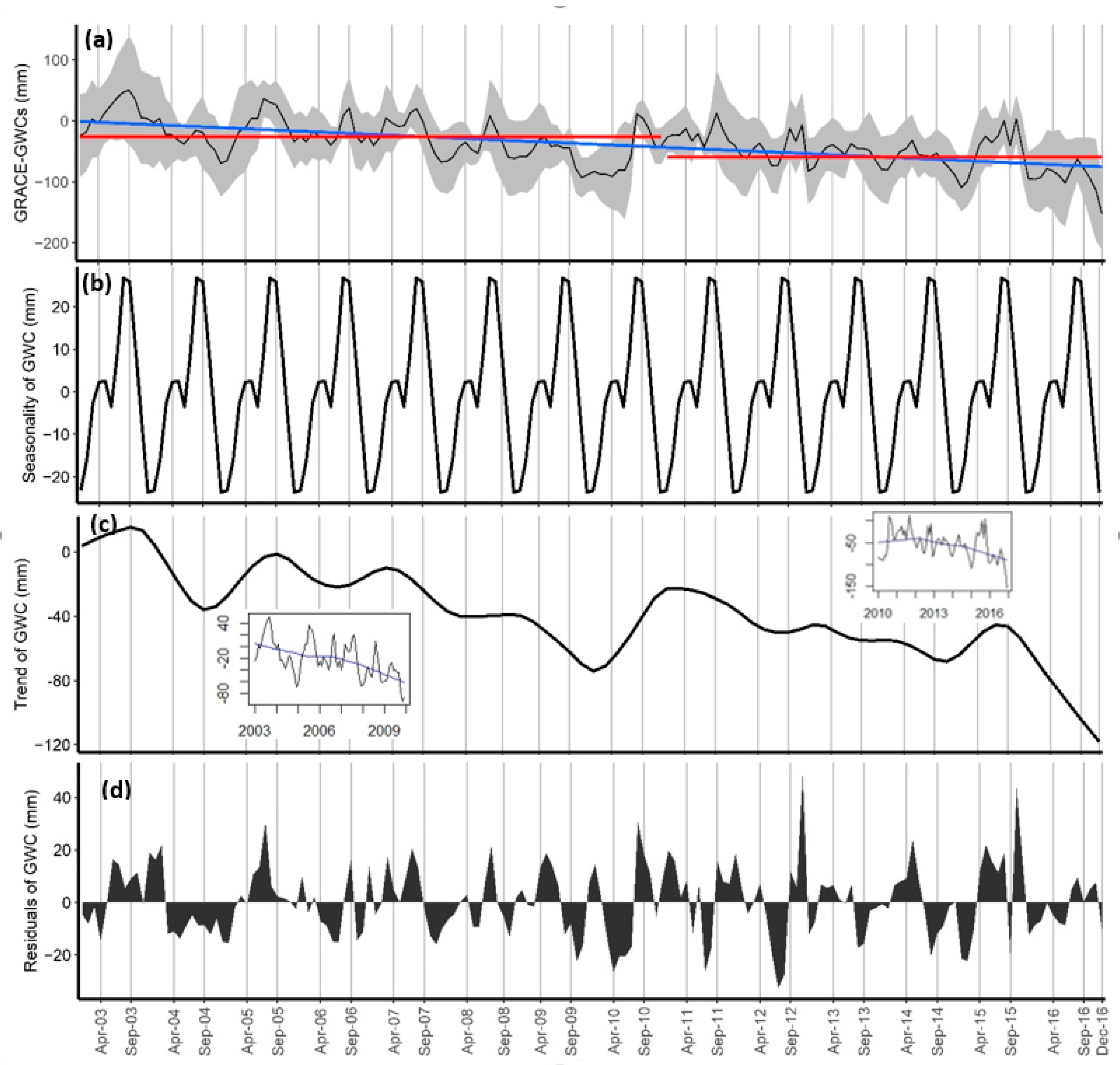
• When analyzed over time, almost all GWC values were negative, with an overall decreasing trend from January 2003 to December 2016. The fluctuations in GWCs were stronger before 2010 than in the second half of the study period. An increase in evapotranspiration was found to be the main controlling factor for the groundwater and total water storage changes across IRB.
• In the spatial analysis, GWC trended downward over the whole Indus Basin. The decline was severe (−131 to −108 mm) in UIB, highlighting a need for sub-basin analysis. We recommend the development of quantitative groundwater aquifer-related maps to visualize water withdrawals, groundwater recharge, groundwater storage changes, groundwater levels, aquifer thickness and yields, and tube well density over the whole IRB. These maps provide useful support to develop area-specific groundwater management strategies.
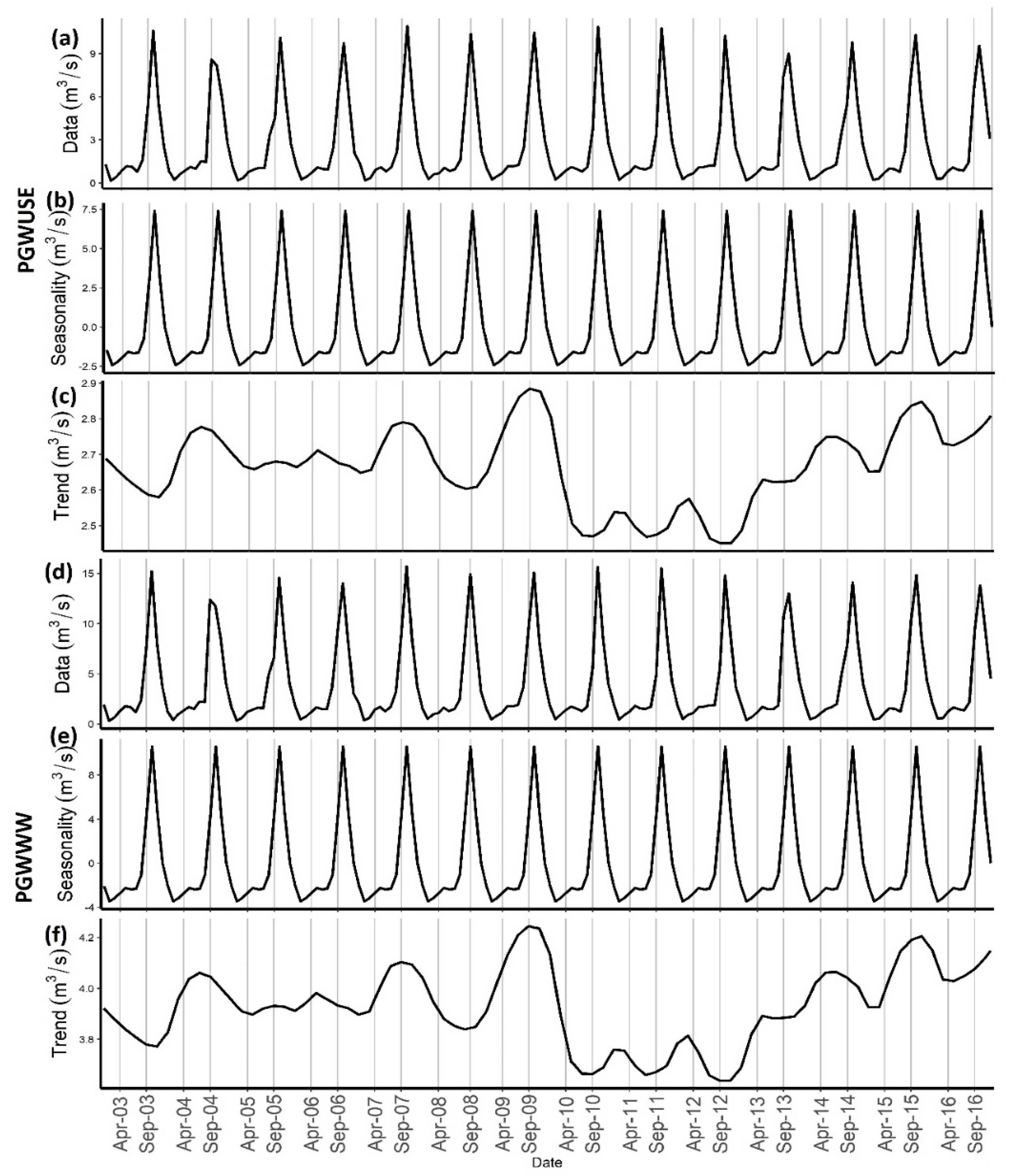
• The reach-specific analysis showed that the upper reach is more vulnerable to groundwater decline compared to the other reaches due to glacier recession. We recommend the adaption of climate mitigation strategies to cater for the climate change impact on glacier recession. This study concludes that groundwater abstraction and groundwater consumption are the most significant driving factors in the middle reach. These results highlight the need for a robust mechanism to monitor the quantity and quality of groundwater abstractions in the middle reach. The outcomes for the lower reach reveal that the high water allowances provided to the canals under WAA 1991 are the main driver of lower groundwater storage change. So, surface water allowances in Pakistan should be allocated based on a detailed understanding of groundwater withdrawals and depletion.
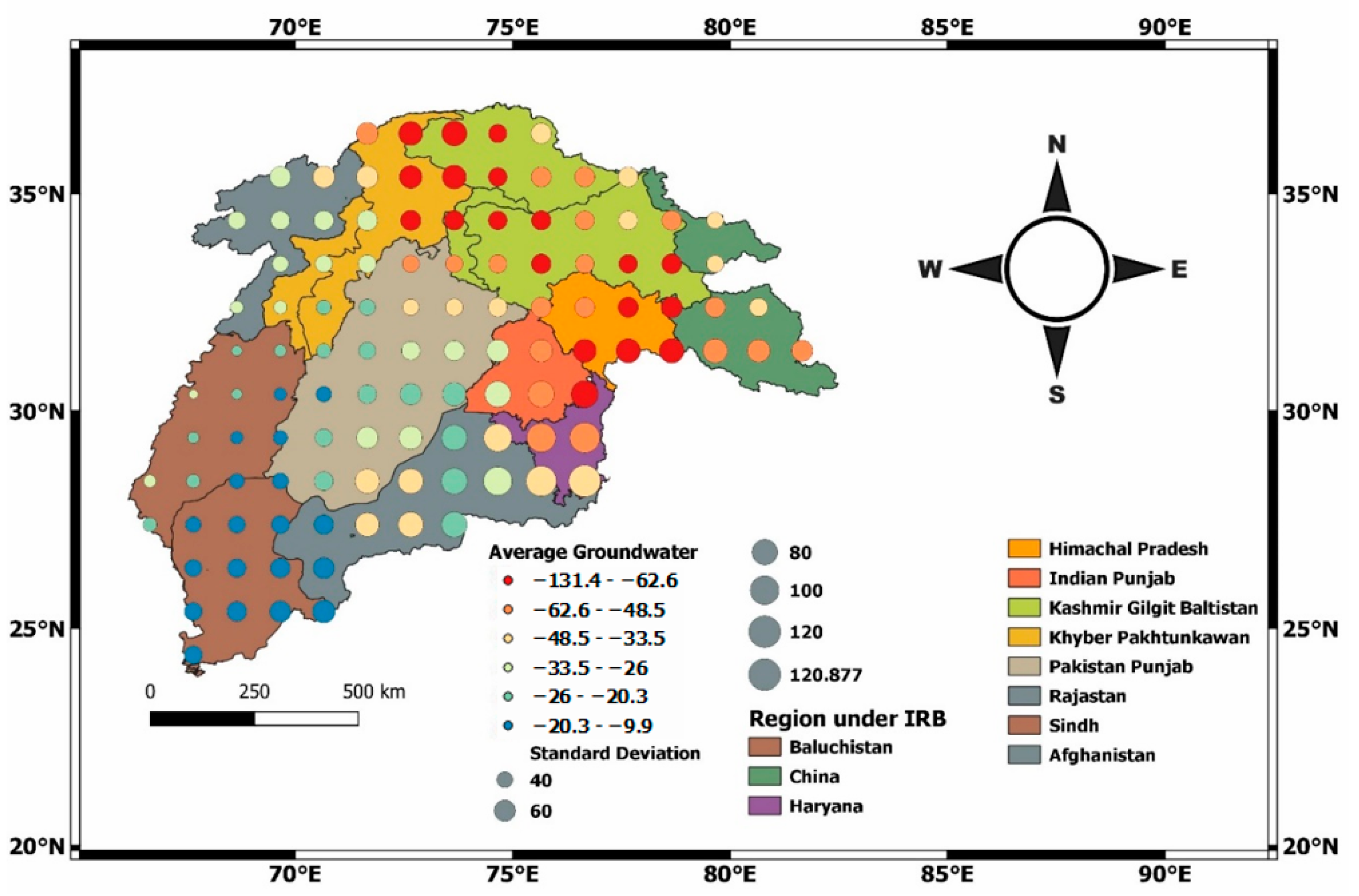
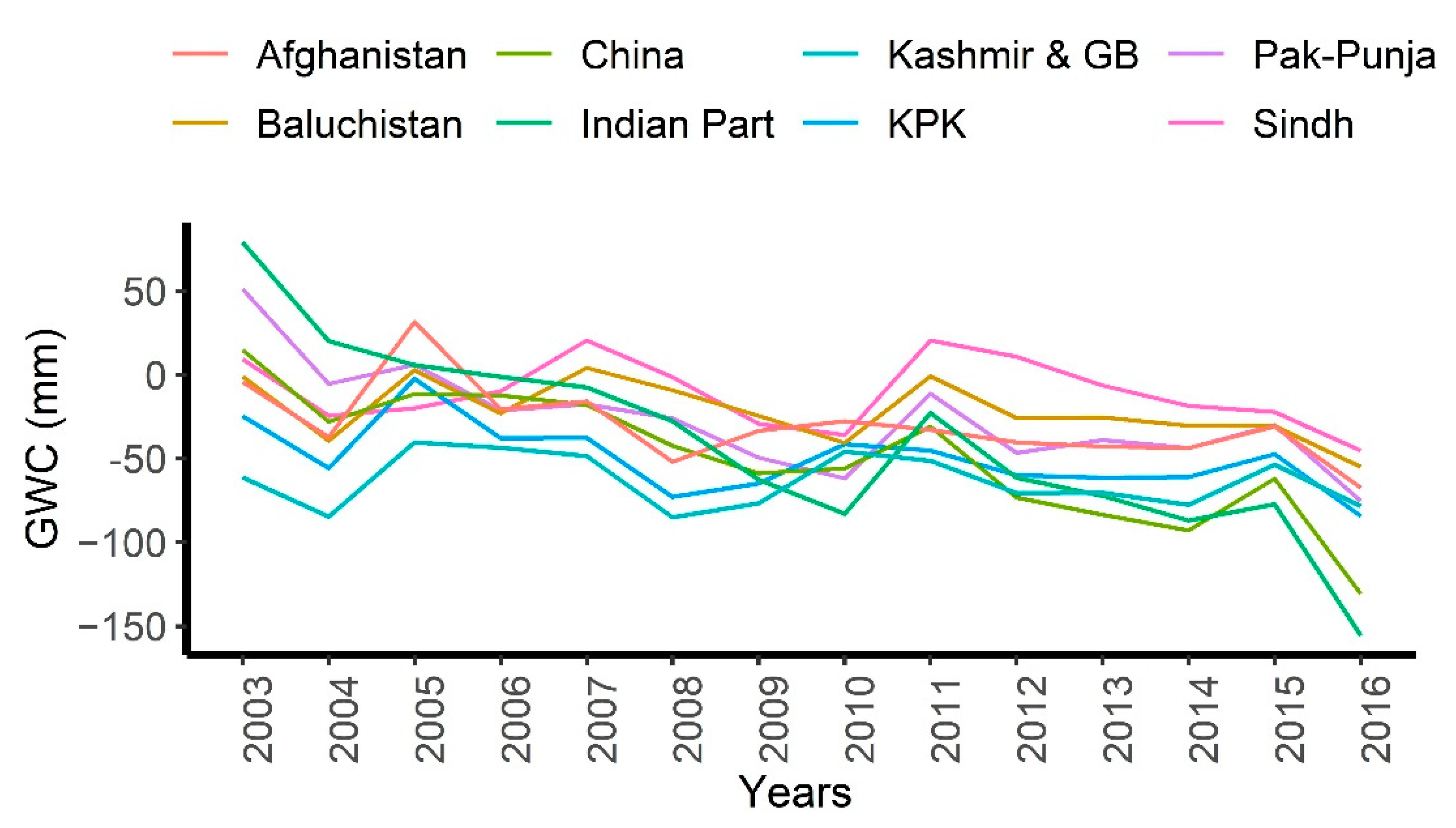
• On the regional scale, the groundwater decline was severe in Himachal Pradesh, Indian Punjab, Haryana, upper Punjab of Pakistan, and China. Due to these regional differences, it is evident that a region-specific groundwater strategic framework is necessary. Hence, a comprehensive mechanism for monitoring and establishing regulatory and permitting arrangements and pricing structures should be developed to envisage sustainable management of the land area and water resources. Because the number and density of tube wells and boreholes have largely increased in recent years, we propose the construction of a database containing georeferenced locations of all existing and new tube wells and boreholes in the regions. Such a database would not only support but also improve management decisions.
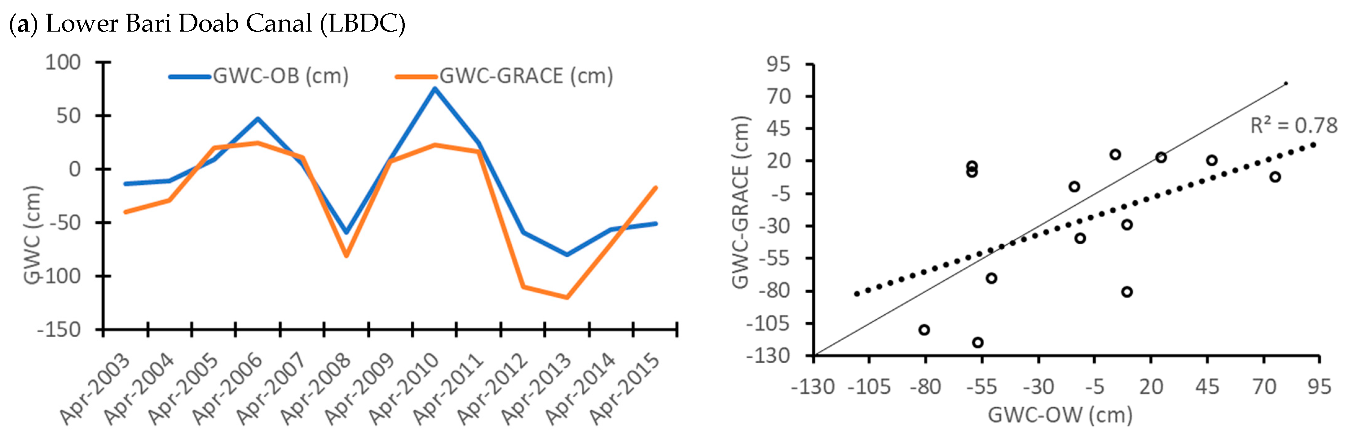
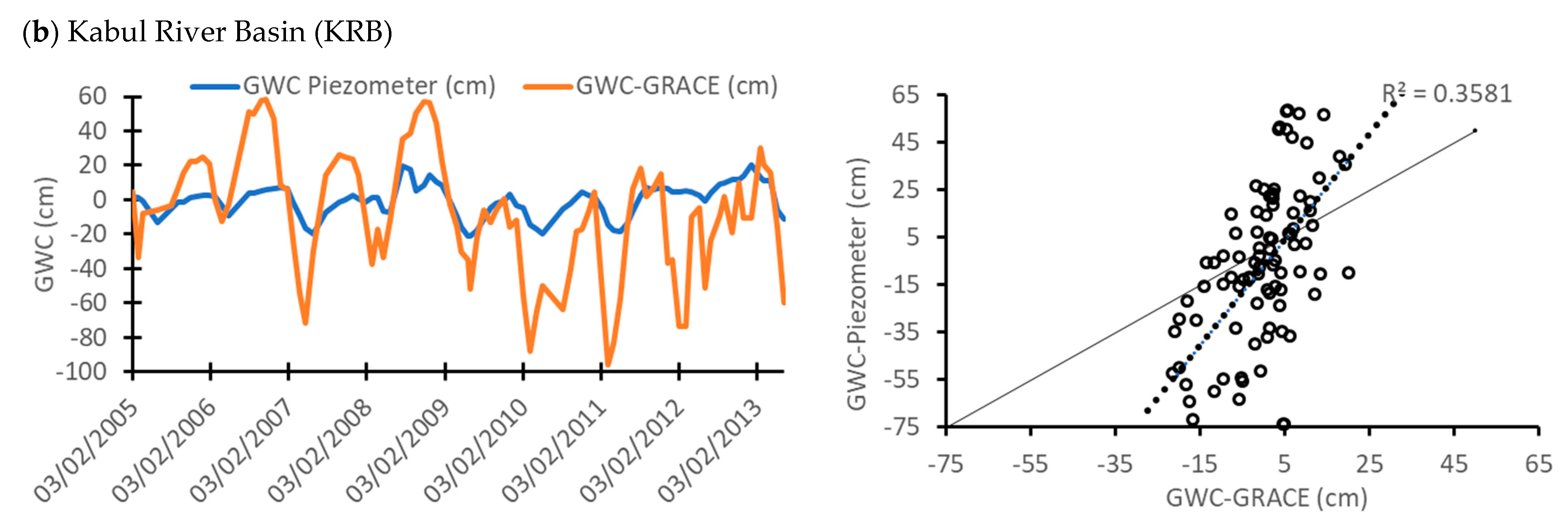
• The correlation between the observed and estimated GWC both at KRB (i.e., R² = 0.35) and LBDC (i.e., R² = 0.78) shows that there are spatial heterogeneities across IRB, which needs to be considered during planning initiatives.

In a nutshell, basin-wide groundwater monitoring infrastructures must be established using the latest technologies (GIS, remote sensing, and Heliborne technology). Such infrastructures are essential for the development of a sound database and maps for groundwater regulation and sustainable management. These will also enable robust monitoring of the quantity and quality of groundwater resources and their use.

References

- Kinzelbach, W.; Bauer, P.; Siegfried, T.; Brunner, P. Sustainable Groundwater Management—Problems and Scientific Tools. Episodes 2003, 26, 279–284. [Google Scholar] [CrossRef] [PubMed]
- Food and Agriculture Organization, Faoa. Irrigation in Southern and Eastern Asia in Figures—AQUASTAT Survey—2011: Indus River Basin; Food and Agriculture Organization: Rome, Italy, 2011; pp. 1–14. [Google Scholar]
- Siebert, S.; Faures, J.M.; Frenken, K.; Hoogeveen, J. Groundwater Use for Irrigation—A Global Inventory. Hydrol. Earth Syst. Sci. 2010, 14, 1863–1880. [Google Scholar] [CrossRef] [Green Version]
- Usman, M.; Qamar, M.U.; Becker, R.; Zaman, M.; Conrad, C.; Salim, S. Numerical Modelling and Remote Sensing Based Approaches for Investigating Groundwater Dynamics under Changing Land-Use and Climate in the Agricultural Region of Pakistan. J. Hydrol. 2020, 581, 124408. [Google Scholar] [CrossRef]
- Cheema, M.J.M.; Immerzeel, W.W.; Bastiaanssen, W.G.M. Spatial Quantification of Groundwater Abstraction in the Irrigated Indus Basin. Groundwater 2014, 52, 25–36. [Google Scholar] [CrossRef] [PubMed] [Green Version]
- Lytton, L.; Ali, A.; Garthwaite, B.; Punthakey, J.F.; Basharat, S. Groundwater in Pakistan’s Indus Basin: Present and Future Prospects. 2021, p. 164. Available online: http://hdl.handle.net/10986/35065 (accessed on 16 April 2021).
- Cheema, M.J.M.; Qamar, M.U. Transboundary Indus River Basin: Potential Threats to Its Integrity; Elsevier Inc.: Amsterdam, The Netherlands, 2019; ISBN 9780128127827. [Google Scholar]
- Arfan, A.; Zhang, Z.; Zhang, W.; Gujree, I. Long-Term Perspective Changes in Crop Irrigation Requirement Caused by Climate and Agriculture Land Use Changes in Rechna Doab, Pakistan. Water 2019, 11, 1567. [Google Scholar] [CrossRef] [Green Version]
- Sun, S.; Zhou, T.; Wu, P.; Wang, Y.; Zhao, X.; Yin, Y. Impacts of Future Climate and Agricultural Land-Use Changes on Regional Agricultural Water Use in a Large Irrigation District of Northwest China. L. Degrad. Dev. 2019, 30, 1158–1171. [Google Scholar] [CrossRef]
- Watto, M.A. The Economics of Groundwater Irrigation in the Indus Basin, Pakistan: Tube-Well Adoption, Technical and Irrigation Water Efficiency and Optimal Allocation. Ph.D. Thesis, University of Western Australia, Crawley WA, Australia, 2015; pp. 1–218. [Google Scholar]
- Qureshi, A.S.; Gill, M.A.; Sarwar, A. Sustainable Groundwater Management in Pakistan: Challenges and Pportunities. Irrig. Drain. 2010, 59, 107–116. [Google Scholar] [CrossRef]
- Lin, M.; Biswas, A.; Bennett, E.M. Spatio-Temporal Dynamics of Groundwater Storage Changes in the Yellow River Basin. J. Environ. Manage. 2019, 235, 84–95. [Google Scholar] [CrossRef] [PubMed]
- Mahmood, R.; JIA, S.; Lv, A.; Zhu, W. A Preliminary Assessment of Environmental Flow in the Three Rivers’ Source Region, Qinghai Tibetan Plateau, China and Suggestions. Ecol. Eng. 2020, 144, 105709. [Google Scholar] [CrossRef]
- Young, W.J.; Arif, A.; Bhatti, T.; Borgomeo, E.; Davies, S.; Garthwaite, W.R., III; Gilmont, E.M.; Leb, C.; Lytton, L.; Makin, I.; et al. Pakistan: Getting More from Water; World Bank: Washington, DC, USA, 2019; p. 163. [Google Scholar]
- Yin, W.; Han, S.C.; Zheng, W.; Yeo, I.Y.; Hu, L.; Tangdamrongsub, N.; Ghobadi-Far, K. Improved Water Storage Estimates within the North China Plain by Assimilating GRACE Data into the CABLE Model. J. Hydrol. 2020, 590, 125348. [Google Scholar] [CrossRef]
- Liu, F.; Kang, P.; Zhu, H.; Han, J.; Huang, Y. Analysis of Spatiotemporal Groundwater-Storage Variations in China from Grace. Water 2021, 13, 2378. [Google Scholar] [CrossRef]
- Rodell, M.; Velicogna, I.; Famiglietti, J.S. Satellite-Based Estimates of Groundwater Depletion in India. Nature 2009, 460, 999–1002. [Google Scholar] [CrossRef] [PubMed] [Green Version]
- Chen, H.; Zhang, W.; Nie, N.; Guo, Y. Long-Term Groundwater Storage Variations Estimated in the Songhua River Basin by Using GRACE Products, Land Surface Models, and in-Situ Observations. Sci. Total Environ. 2019, 649, 372–387. [Google Scholar] [CrossRef]
- Tapley, B.D.; Bettadpur, S.; Watkins, M.; Reigber, C. The Gravity Recovery and Climate Experiment: Mission Overview and Early Results. Geophys. Res. Lett. 2004, 31, L09607. [Google Scholar] [CrossRef] [Green Version]
- Iqbal, N.; Hossain, F.; Lee, H.; Akhter, G. Integrated Groundwater Resource Management in Indus Basin Using Satellite Gravimetry and Physical Modeling Tools. Environ. Monit. Assess. 2017, 189, 128. [Google Scholar] [CrossRef] [PubMed]
- Iqbal, N.; Hossain, F.; Lee, H.; Akhter, G. Satellite Gravimetric Estimation of Groundwater Storage Variations over Indus Basin in Pakistan. IEEE J. Sel. Top. Appl. Earth Obs. Remote Sens. 2016, 9, 3524–3534. [Google Scholar] [CrossRef]
- Tang, Y.; Hooshyar, M.; Zhu, T.; Ringler, C.; Sun, A.Y.; Long, D.; Wang, D. Reconstructing Annual Groundwater Storage Changes in a Large-Scale Irrigation Region Using GRACE Data and Budyko Model. J. Hydrol. 2017, 551, 397–406. [Google Scholar] [CrossRef]
- Fallatah, O.A.; Ahmed, M.; Save, H.; Akanda, A.S. Quantifying Temporal Variations in Water Resources of a Vulnerable Middle Eastern Transboundary Aquifer System. Hydrol. Process. 2017, 31, 4081–4091. [Google Scholar] [CrossRef]
- Ghebreyesus, D.; Temimi, M.; Fares, A.; Bayabil, H. A Multi-Satellite Approach for Water Storage Monitoring in an Arid Watershed. Geosciences 2016, 6, 33. [Google Scholar] [CrossRef] [Green Version]
- Huang, X.; Gao, L.; Crosbie, R.S.; Zhang, N.; Fu, G.; Doble, R. Groundwater Recharge Prediction Using Linear Regression, Multi-Layer Perception Network, and Deep Learning. Water 2019, 11, 1879. [Google Scholar] [CrossRef]
- Verma, K.; Katpatal, Y.B. Groundwater Monitoring Using GRACE and GLDAS Data after Downscaling Within Basaltic Aquifer System. Ground Water 2019, 58, 143–151. [Google Scholar] [CrossRef]
- Srivastava, S.; Dikshit, O. Seasonal and Trend Analysis of TWS for the Indo-Gangetic Plain Using GRACE Data. Geocarto Int. 2020, 35, 1343–1359. [Google Scholar] [CrossRef]
- Papa, F.; Frappart, F.; Malbeteau, Y.; Shamsudduha, M.; Vuruputur, V.; Sekhar, M.; Ramillien, G.; Prigent, C.; Aires, F.; Pandey, R.K.; et al. Satellite-Derived Surface and Sub-Surface Water Storage in the Ganges-Brahmaputra River Basin. J. Hydrol. Reg. Stud. 2015, 4, 15–35. [Google Scholar] [CrossRef] [Green Version]
- Moghim, S. Assessment of Water Storage Changes Using GRACE and GLDAS. Water Resour. Manag. 2020, 34, 685–697. [Google Scholar] [CrossRef]
- Li, H.; Lu, Y.; Zheng, C.; Zhang, X.; Zhou, B.; Wu, J. Seasonal and Inter-Annual Variability of Groundwater and Their Responses to Climate Change and Human Activities in Arid and Desert Areas: A Case Study in Yaoba Oasis, Northwest China. Water 2020, 12, 303. [Google Scholar] [CrossRef] [Green Version]
- Zhu, Y.; Liu, S.; Yi, Y.; Qi, M.; Li, W.; Saifullah, M.; Zhang, S.; Wu, K. Spatio-Temporal Variations in Terrestrial Water Storage and Its Controlling Factors in the Eastern Qinghai-Tibet Plateau. Hydrol. Res. 2021, 52, 323–338. [Google Scholar] [CrossRef]
- Huang, Y.; Salama, M.S.; Krol, M.S.; Su, Z.; Hoekstra, A.Y.; Zeng, Y.; Zhou, Y. Estimation of Human-Induced Changes in Terrestrial Water Storage through Integration of GRACE Satellite Detection and Hydrological Modeling: A Case Study of the Yangtze River Basin. Water Resour. Res. 2015, 51, 8494–8516. [Google Scholar] [CrossRef]
- World Bank The Indus Waters Treaty 1960 (with Annexes). Signed at Karachi, on 19 September 1960. United Nations—Treaty Ser. 1962, 6032, 1–85. [Google Scholar]
- IRSA Apportionment of Waters of Indus River System between the Provinces of Pakistan. Indus River Syst. Auth. Gov. Pak. 1992, 1–47.
- Ali, S.; Liu, D.; Fu, Q.; Cheema, M.J.M.; Pham, Q.B.; Rahaman, M.M.; Dang, T.D.; Anh, D.T. Improving the Resolution of Grace Data for Spatio-Temporal Groundwater Storage Assessment. Remote Sens. 2021, 13, 3513. [Google Scholar] [CrossRef]
- Shekhar, S.; Mao, R.S.K.; Imchen, E.B. Groundwater Management Options in North District of Delhi, India: A Groundwater Surplus Region in over-Exploited Aquifers. J. Hydrol. Reg. Stud. 2015, 4, 212–226. [Google Scholar] [CrossRef] [Green Version]
- Ali, S.; Wang, Q.; Liu, D.; Fu, Q.; Mafuzur Rahaman, M.; Abrar Faiz, M.; Jehanzeb Masud Cheema, M. Estimation of Spatio-Temporal Groundwater Storage Variations in the Lower Transboundary Indus Basin Using GRACE Satellite. J. Hydrol. 2022, 605, 127315. [Google Scholar] [CrossRef]
- Akhtar, F.; Nawaz, R.A.; Hafeez, M.; Awan, U.K.; Borgemeister, C.; Tischbein, B. Evaluation of GRACE Derived Groundwater Storage Changes in Different Agro-Ecological Zones of the Indus Basin. J. Hydrol. 2022, 605, 127369. [Google Scholar] [CrossRef]
- Arshad, A.; Mirchi, A.; Samimi, M.; Ahmad, B. Combining Downscaled-GRACE Data with SWAT to Improve the Estimation of Groundwater Storage and Depletion Variations in the Irrigated Indus Basin (IIB). Sci. Total Environ. 2022, 838, 156044. [Google Scholar] [CrossRef] [PubMed]
- Archer, D.R.; Forsythe, N.; Fowler, H.J.; Shah, S.M. Sustainability of Water Resources Management in the Indus Basin under Changing Climatic and Socio Economic Conditions. Hydrol. Earth Syst. Sci. 2010, 14, 1669–1680. [Google Scholar] [CrossRef] [Green Version]
- Iqbal Abdul Rauf Environmental Issues of Indus River Basin: An Analysis. ISSRA Pap. Inst. Strateg. Stud. Res. Anal. (ISSRA) Natl. Def. Univ. Islam. Pak. 2013, 5, 91–112.
- Landerer, F.W.; Swenson, S.C. Accuracy of Scaled GRACE Terrestrial Water Storage Estimates. Water Resour. Res. 2012, 48, 1–11. [Google Scholar] [CrossRef]
- Landerer, F. GFZ TELLUS GRACE Level-3 Monthly LAND Water-Equivalent-Thickness Surface-Mass Anomaly Release 6.0 in NetCDF/ASCII/GeoTIFF Formats. Ver. 6.0. PO.DAAC, CA, USA. Available online: Https://Doi.Org/10.5067/TELND-3AG06 (accessed on 17 December 2019).
- Landerer, F. CSR TELLUS GRACE Level-3 Monthly LAND Water-Equivalent-Thickness Surface-Mass Anomaly Release 6.0 in NetCDF/ASCII/GeoTIFF Formats. Ver. 6.0. PO.DAAC, CA, USA. Available online: Https://Doi.Org/10.5067/TELND-3AC06 (accessed on 17 December 2019).
- Landerer, F. JPL TELLUS GRACE Level-3 Monthly LAND Water-Equivalent-Thickness Surface-Mass Anomaly Release 6.0 in NetCDF/ASCII/GeoTIFF Formats. Ver. 6.0. PO.DAAC, CA, USA. Available online: Https://Doi.Org/10.5067/TELND-3AJ06 (accessed on 4 December 2019).
- Rodell, M.; Beaudoing, H. GLDAS CLM Land Surface Model L4 Monthly 1.0 × 1.0 Degree V001; Goddard Earth Sciences Data and Information Services Center: Greenbelt, MD, USA, 2007. [Google Scholar]
- Müller Schmied, H.; Cáceres, D.; Eisner, S.; Flörke, M.; Herbert, C.; Niemann, C.; Peiris, T.A.; Popat, E.; Portmann, F.T.; Reinecke, R.; et al. The Global Water Resources and Use Model WaterGAP v2.2d: Model Description and Evaluation. Geosci. Model Dev. Discuss. 2021, 14, 1037–1079. [Google Scholar] [CrossRef]
- Feng, W.; Shum, C.K.; Zhong, M.; Pan, Y. Remote Sensing Groundwater Storage Changes in China from Satellite Gravity: An Overview. Remote Sens. 2018, 10, 674. [Google Scholar] [CrossRef] [Green Version]
- Huffman, G.J.; Bolvin, D.T.; Nelkin, E.J. Integrated Multi-SatellitE Retrievals for GPM (IMERG), Version 4.4. NASA’s Precipitation Processing Center. Available online: https://gpm.nasa.gov/data/policy (accessed on 6 February 2021).
- Voss, K.A.; Famiglietti, J.S.; Lo, M.; De Linage, C.; Rodell, M.; Swenson, S.C. Groundwater Depletion in the Middle East from GRACE with Implications for Transboundary Water Management in the Tigris-Euphrates-Western Iran Region. Water Resour. Res. 2013, 49, 904–914. [Google Scholar] [CrossRef] [Green Version]
- Frappart, F.; Ramillien, G. Monitoring Groundwater Storage Changes Using the Gravity Recovery and Climate Experiment (GRACE) Satellite Mission: A Review. Remote Sens. 2018, 10, 829. [Google Scholar] [CrossRef] [Green Version]
- Yin, W.; Hu, L.; Jiao, J.J. Evaluation of Groundwater Storage Variations in Northern China Using GRACE Data. Geofluids 2017, 2017, 8254824. [Google Scholar] [CrossRef] [Green Version]
- Cleveland, R.B.; William, S.; Cleveland, J.E.; McRAe, I.T. STL: A Seasonal-Trend Decomposition Procedure Based on Loess. J. Off. Stat. 1990, 6, 3–73. [Google Scholar]
- Shamsudduha, M.; Chandler, R.E.; Taylor, R.G.; Ahmed, K.M. Recent Trends in Groundwater Levels in a Highly Seasonal Hydrological System: The Ganges-Brahmaputra-Meghna Delta. Hydrol. Earth Syst. Sci. 2009, 13, 2373–2385. [Google Scholar] [CrossRef]
- Buma, W.G.; Lee, S.I.; Seo, J.Y. Hydrological Evaluation of Lake Chad Basin Using Space Borne and Hydrological Model Observations. Water 2016, 8, 205. [Google Scholar] [CrossRef] [Green Version]
- Taher, M.R.; Chornack, M.P.; Mack, T.J. Groundwater Levels in the Kabul Basin, Afghanistan, 2004–2013; U.S. Department of the Interior, U.S. Geological Survey: Reston, VA, USA, 2014.
- Yu, W.; Yang, Y.-C.; Savitsky, A.; Alford, D.; Brown, C.; Wescoat, J.; Debowicz, D.; Robinson, S. The Indus Basin of Pakistan; The World Bank: Washington, DC, USA, 2013. [Google Scholar]
- Federal Flood Commission, Ministry of Water Resources. Annual Flood Report 2017. 2017. Available online: https://mowr.gov.pk/SiteImage/Misc/files/2017%20Annual%20Flood%20Report%20of%20FFC.pdf (accessed on 20 February 2020).
- Muhammad, S.; Tian, L.; Khan, A. Early Twenty-First Century Glacier Mass Losses in the Indus Basin Constrained by Density Assumptions. J. Hydrol. 2019, 574, 467–475. [Google Scholar] [CrossRef]
- Basharat, M.; Ali, S.U.; Azhar, A.H. Spatial Variation in Irrigation Demand and Supply across Canal Commands in Punjab: A Real Integrated Water Resources Management Challenge. Water Policy 2014, 16, 397–421. [Google Scholar] [CrossRef]
- Ali, S.; Cheema, M.J.M.; Waqas, M.M.; Waseem, M.; Awan, U.K.; Khaliq, T. Changes in Snow Cover Dynamics over the Indus Basin: Evidences from 2008 to 2018 MODIS NDSI Trends Analysis. Remote Sens. 2020, 12, 2782. [Google Scholar] [CrossRef]
- Qureshi, A.S.; Shah, T.; Akhtar, M. The Groundwater Economy of Pakistan; IWMI: Colombo, Sri Lanka, 2003; p. 31. [Google Scholar]
- Qureshi, A.S. Groundwater Governance in Pakistan: From Colossal Development to Neglected Management. Water 2020, 12, 3017. [Google Scholar] [CrossRef]
- Mishra, V.; Asoka, A.; Vatta, K.; Lall, U. Groundwater Depletion and Associated CO2 Emissions in India. Earth’s Futur. 2018, 6, 1672–1681. [Google Scholar] [CrossRef]
- NASA NASA Satellites Unlock Secret to Northern India’s Vanishing Water. Available online: https://www.nasa.gov/topics/earth/features/india_water.html (accessed on 3 February 2021).
- Chen, J.; Famigliett, J.S.; Scanlon, B.R.; Rodell, M. Groundwater Storage Changes: Present Status from GRACE Observations. Surv. Geophys. 2016, 37, 397–417. [Google Scholar] [CrossRef] [Green Version]
- Baweja, S.; Aggarwal, R.; Brar, M. Groundwater Depletion in Punjab, India. Encycl. Soil Sci. Third Ed. 2017, 1–5. [Google Scholar] [CrossRef]
- Shah, T.; Roy, A.D.; Qureshi, A.S.; Wang, J. Sustaining Asia’s Groundwater Boom: An Overview of Issues and Evidence. Nat. Resour. Forum 2003, 27, 130–141. [Google Scholar] [CrossRef] [Green Version]
- Asoka, A.; Gleeson, T.; Wada, Y.; Mishra, V. Relative Contribution of Monsoon Precipitation and Pumping to Changes in Groundwater Storage in India. Nat. Geosci. 2017, 10, 109–117. [Google Scholar] [CrossRef]
- Singh, A.P.; Bhakar, P. Development of Groundwater Sustainability Index: A Case Study of Western Arid Region of Rajasthan, India. Environ. Dev. Sustain. 2020, 23, 1844–1868. [Google Scholar] [CrossRef]
- van Steenbergen, F.; Kaisarani, A.B.; Khan, N.U.; Gohar, M.S. A Case of Groundwater Depletion in Balochistan, Pakistan: Enter into the Void. J. Hydrol. Reg. Stud. 2015, 4, 36–47. [Google Scholar] [CrossRef] [Green Version]
- Yin, W.; Li, T.; Zheng, W.; Hu, L.; Han, S.C.; Tangdamrongsub, N.; Šprlák, M.; Huang, Z. Improving Regional Groundwater Storage Estimates from GRACE and Global Hydrological Models over Tasmania, Australia. Hydrogeol. J. 2020, 28, 1809–1825. [Google Scholar] [CrossRef]
- Feng, T.; Shen, Y.; Chen, Q.; Wang, F.; Zhang, X. Groundwater Storage Change and Driving Factor Analysis in North China Using Independent Component Decomposition. J. Hydrol. 2022, 609, 127708. [Google Scholar] [CrossRef]
- Alley, W.M.; Konikow, L.F. Bringing GRACE Down to Earth. Groundwater 2015, 53, 826–829. [Google Scholar] [CrossRef]