
Influence of the Gyeongju Earthquake on Observed Groundwater Levels at a Power Plant
KEPCO International Nuclear Graduate School, Ulsan 45014, Korea
*
Author to whom correspondence should be addressed.
Water 2022, 14(20), 3229; https://doi.org/10.3390/w14203229
Submission received: 29 July 2022
/
Revised: 2 October 2022
/
Accepted: 8 October 2022
/
Published: 13 October 2022
(This article belongs to the Special Issue How Earthquakes Affect Groundwater)
Abstract
:Groundwater levels at a power plant site were analyzed using statistical techniques to ascertain if there was any influence from an earthquake that occurred approximately 27 km away. This earthquake was the Mw 5.5 Gyeongju earthquake that occurred on 12 September 2016 at 11:32 UTC in South Korea. Groundwater levels at five groundwater monitoring wells were examined against the 2016 Gyeongju earthquake, local precipitation, and local tide levels. A visual examination of the groundwater monitoring well data suggested no real effect or influence from the earthquake. However, precipitation data implied a rise in groundwater levels. Cross-correlation analyses also showed no significant relationship between groundwater levels and the earthquake in question. Interestingly, three of the five groundwater monitoring wells suggested a low-to-moderate correlation between groundwater and tide levels while the remaining two groundwater monitoring wells showed a low-to-moderate correlation between groundwater levels and precipitation. Granger causality tests suggested a closer relationship between tide and groundwater levels for two of the wells, questionable results describing precipitation for another two wells, and no relationship with the earthquake for four of the wells. Data resolution plays an important role in the analyses.
1. Introduction
Depending on the type of power plant, many require access to a variety of water resources for operations and maintenance. Some plant operations need to consider groundwater levels, for example with regard to water supply, water contamination, pipe leakages, or even carbon capture and sequestration [1,2,3,4]. The common scenario is where a subsurface pipe or tank is damaged, either through earthquake shaking or age, forcing a leak. An increase in groundwater levels would assist in the transport of the effluent. Additionally, with regard to certain materials such as concrete, when groundwater levels rise and fall, the water may cause additional reactions such as the dissolution of calcium carbonate or the transport of foreign minerals into and onto the facing. For example, the Wolseong Low and Intermediate Level Radioactive Waste Disposal Center in South Korea (Republic of Korea) is an underground repository constructed with a concrete liner containment system, which can degrade and become more porous over time [5]. This implies the potential leakage and transport of hazardous materials into the groundwater. Conversely, during emergency situations, a power plant might require additional water pumped from groundwater resources. Sudden and drastic changes in groundwater levels may hinder a power plant operator from doing so. Even though groundwater levels are typically influenced by precipitation and infiltration, there have been considerations on how and to what extent an earthquake can influence groundwater levels.
Three types of groundwater level behavior have been observed during seismic activity. One is where no change is observed. Another is where groundwater levels exhibit oscillatory behavior that diminishes shortly after the earthquake is over, returning to base flow [6,7]. The other is where groundwater levels show an abrupt offset, rise, or fall, which usually lasts well past the earthquake and in certain instances returns to a different base flow level [8,9,10]. The hypothesized mechanisms for these changes in groundwater levels due to an earthquake are complex, citing principles from hydrology and soil mechanics, as well as earthquake engineering [6,7,8,9,10,11]. One of the more comprehensive yet simple hypothetical mechanisms originates from the fundamentals of groundwater flow. For example, groundwater flow in an unconfined aquifer is described by the equation:
where Kx, Ky, and Kz = the values of hydraulic conductivity in the x, y, and z directions, respectively, along Cartesian coordinate axes, which is the volumetric flow per unit of time per cross-sectional unit area of the aquifer; h = hydraulic head; W = volumetric flux per unit volume which represents sinks or sources; t = time; and S = the storativity or storage coefficient of the porous material, which is equal to SSB + Sy, where Sy is the specific yield of the aquifer materials, B = the thickness of the aquifer, and SS = the specific storage of the porous material. The specific storage is:
where γw = the specific weight of water; n = the porosity of the material; βp = the compressibility of the bulk aquifer material; and βw = the compressibility of water. Note that:
where Vt = total volume or the control volume; σe = effective stress; Vw = volume of water; and p = pore water pressure. These basically describe the change in total volume or water volume per change with applied stress. The unconfined groundwater table is typically derived from the hydraulic head solution to Equation (1). Different assumptions and constraints to Equation (1) allow for simplification and analytic solutions.
The general hypothesis is that propagating seismic waves cause cyclic strains in the aquifer materials. These strains result in deformation and displacement, possibly causing micro-cracking as well as the removal of particles occupying fractures [6,12,13,14,15]. Such behavior could potentially increase or decrease the hydraulic conductivity of the aquifer, as shown on the left side of Equation (1). Moreover, such straining and stressing may affect the compressibility of the aquifer materials, as on the right side of Equation (1). The idea is that changes in the effective stress term in Equation (3) would affect Equation (2). Additionally, the ground motions, as well as responses in the aquifers, will cause oscillatory pore water pressure changes, which affect the hydraulic head, possibly forcing flow into or out of the aquifer materials. This is also accounted for by Equation (4) where changes in pore water pressure would also affect the storativity of the aquifer. Interestingly, this induced flow may also facilitate the unclogging of microfractures, thereby increasing hydraulic conductivity. However, it should be noted that the compressibility of water, as defined in Equation (4), is generally considered low under normal conditions and that Sy is typically much larger than SS in practice. Nonetheless, the mechanics allow for observation.
This makes the 2016 Gyeongju earthquake a valuable example of groundwater levels and seismic activity. The 12 September 2016, 11:32 UTC, MW = 5.5 Gyeongju earthquake epicenter was located nearby important industrial facilities, such as large power plants as well as the Wolseong Low and Intermediate Level Radioactive Waste Disposal Center. Prior to this event, the stable continental region had relatively few earthquakes of magnitudes MW > 5.0 [16,17,18]. Interestingly, this event was preceded by several foreshocks, the largest being an MW = 5.1 event on 12 September 2016 at 10:44 UTC, approximately 11 km southwest of the epicenter of the main shock [17,18,19]. Figure 1 shows the earthquake epicenter and Modified Mercalli Intensity (MMI) scale intensity contours [16]. Earthquake intensity measures the effects of earthquakes as observed by people. The MMI scale is from 1 to 12, with higher intensities indicative of extreme shaking and damage [20,21]. For the 2016 Gyeongju earthquake, the intensity contours ranged from 4 to 5.5, with a reported maximum of 7, and covered a wide region in the southeastern area of South Korea. The 2016 Gyeongju foreshocks had similar MMI contours, but at a lower range of 3.5 to 5.5, with a reported maximum of 6. The effects of the 2016 Gyeongju earthquake were broadcast on major television shows and there was significant coverage commenting if South Korea was seismically safe or how resilient South Korea was to potentially larger earthquakes, especially considering the ongoing effects of the 2011 Fukushima disaster.
There has been some work on the correlation between groundwater level changes and the 2016 Gyeongju earthquake [23,24,25,26]. These studies use data from several and sometimes overlapping groundwater monitoring wells within 50 km of the epicenter. In addition to groundwater levels, some of these studies also showed precipitation, water temperature, and electrical conductivity measurements. Their findings suggest that at least one groundwater monitoring well showed a response to the 2016 Gyeongju earthquake. However, some of these studies showed bias, as any increase in groundwater levels during the time of the earthquake implied causation. Furthermore, some of these studies did not particularly account for precipitation, especially when considering other periods in their groundwater level records also showed decreasing and stagnant groundwater levels during precipitation. Studies that did apply filtering and modeling showed these might have introduced additional bias [24,25]. Moreover, when available, comparisons of monitoring well host materials seemed inconsistent. For example, one study found only the monitoring well founded in bedrock to show a response to the earthquake, but other similarly located monitoring wells founded in more shallow soil materials with higher hydraulic conductivities did not [24,25]. However, it is noted that many of these groundwater monitoring wells are founded in undeveloped areas [24,25,26].
In addition to considerations on the influence of earthquakes on groundwater levels, there are also studies on the behavior of groundwater levels as a precursor to seismic activity [26,27,28,29,30,31,32,33]. The motivating concept is that changes due to seismic activity, such as a foreshock, will induce ground strains and deformations that allow for groundwater level changes. These may be abnormal increases or decreases in groundwater levels. Many of these earthquake prediction studies also consider other parameters in addition to groundwater level changes, such as geochemistry, temperature, or emissions. In this area, the literature is mostly composed of work that supports the prediction of earthquakes using groundwater levels along with another natural parameter, usually chemical in nature [34,35]. One study suggested the installation of additional groundwater monitoring wells to help with earthquake forecasting, but then that would beg the question of acceptance criteria for an upcoming earthquake [25]. Another study offered a magnitude-dependent relationship for observable differences [27]. These could be crucial for critical power plants as well as radioactive waste repositories.
Given this backdrop, this investigation has two objectives in mind. One is to examine if the 2016 Gyeongju earthquake influenced groundwater levels at a nearby power plant using statistical methods. As presented earlier, power plants and related infrastructure have special water resource needs and are typically in highly developed environments, quite different from the typical monitoring well environment. Another objective is to examine if groundwater levels at a nearby power plant could reasonably forecast the 2016 Gyeongju earthquake. A review of groundwater level readings from power plant groundwater monitoring wells is compared to the earthquake event, local precipitation, and tidal measurements. The scope does not include observations in water chemistry, gaseous chemistry, or wildlife observations, nor is the explicit consideration of groundwater monitoring wells outside the power plant of interest. Hopefully, these results will add to a database on the nexus of groundwater hydrology and earthquakes as well as shed some insight into these effects at major plant sites.
2. Materials and Methods
2.1. Study Site
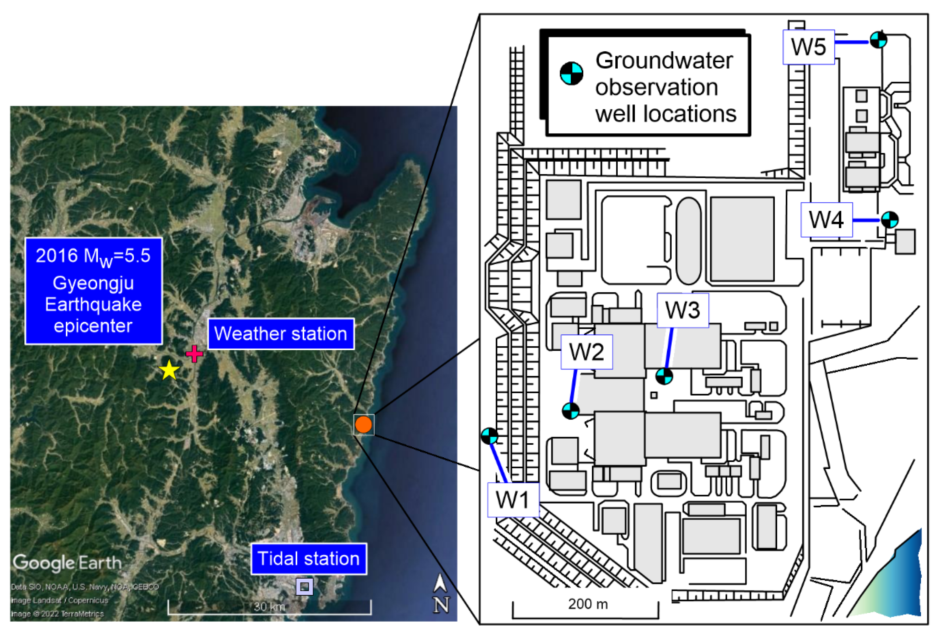
This study focuses on the groundwater monitoring wells installed at a power plant near the 2016 Gyeongju earthquake epicenter, as shown in Figure 2. The distance from the epicenter to the power plant is about 27 km. The developed site is relatively flat with a majority covered by concrete and concrete mixes, with concrete drainage conduits installed around the plant site. The figure indicates five groundwater monitoring wells, W1 to W5, scattered across the site. All wells use a CTD-Diver submersible datalogger to record water levels at intervals of 1 h inside the wells. The datalogger provided recordings at a resolution of 1 cmH2O with an accuracy of ±2.5 cmH2O. These monitoring wells extended approximately 60 cm above the ground service, vented and capped, in weatherproof structures to prevent the interference of rain or other debris. Compensation for barometric pressure was derived from recordings from a Baro-Diver datalogger with a pressure accuracy of ±0.5 cmH2O. Groundwater monitoring well W1 is the highest, at a ground elevation of around 40 m above mean sea level with the sensor installed at 16 m above mean sea level. Groundwater monitoring well W2 is at a ground elevation of around 10 m above mean sea level with the sensor installed at 8 m below mean sea level. Groundwater monitoring wells W3 through W5 are at a ground elevation of around 11 m above mean sea level with the sensor installed at 8 m below mean sea level. Wells W4 and W5 are closest to the ocean and well W1 is furthest from the ocean. Due to the local geology and the construction of the power plant, groundwater monitoring well W1 was founded in fill while groundwater monitoring wells W2 through W5 were founded in bedrock. More detailed construction details of the groundwater monitoring wells were unavailable at the time of this analysis.
Complementing groundwater table observations, relevant precipitation recordings in the local area are also considered. These data are available from the Korean Meteorological Agency [36]. Since the scope of this study is concerned with the impact the 2016 Gyeongju earthquake had on groundwater levels, only data from the month of September are considered.
Additionally, since the site is near the ocean, recorded tidal data near the site are also available from the Korea Hydrographic and Oceanographic Agency [37]. Hourly tide levels are recorded at the Ulsan tide observatory in Ulsan city, approximately 25 km south of the plant site. These data help in determining if ocean tides have any significant influence on groundwater levels at the plant. Similar to precipitation, only data in the month of September are considered.
As previously mentioned, to help avoid bias, statistical methods will be applied to the power plant site data to help ascertain if the earthquakes caused groundwater level changes. These methods are cross-correlation analysis and the Granger causality test.
2.2. Cross-Correlation Analysis
The technique essentially delays one time series against the other and then calculates the Pearson correlation coefficient for the adjusted series, with the Pearson correlation coefficient, r, being:
where y and x = time series data; μy and μx = average of the y and x time series, respectively; i = time series element index; N = total number of data elements in the time series; lag = the delay in the index of the time series. This technique assumes that the original time series are equally spaced and identical in the number of elements. When using the complete data series, the number of elements in time series y is shifted accordingly to account for the lagged x series.
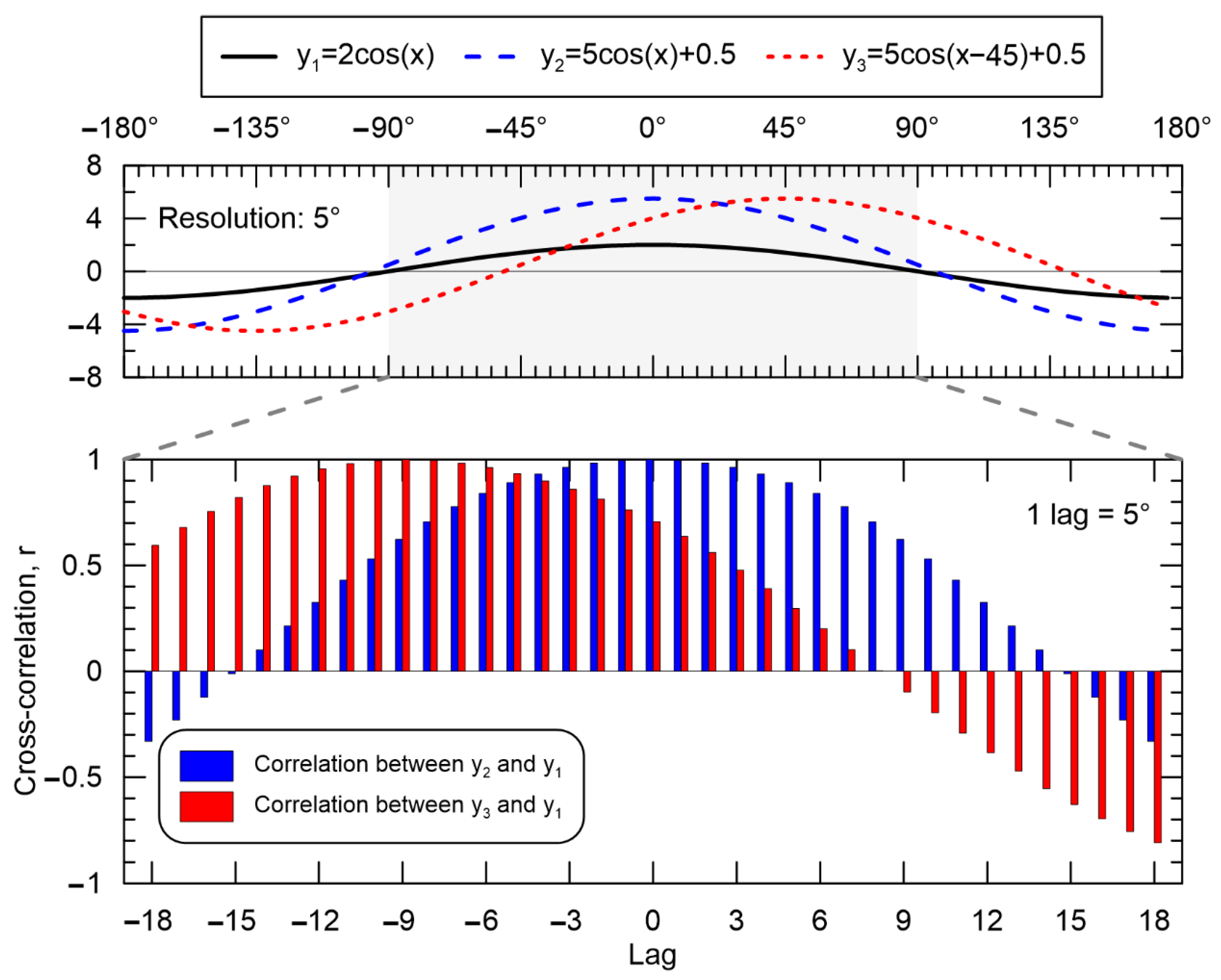
As an example, Figure 3 plots three series to help visualize cross-correlation analysis. The top part of the figure shows the harmonic functions y1 = 2cos(x), y2 = 5cos(x) + 0.5, and y3 = 5cos(x + 45) + 0.5. The bottom part of the figure shows the results of cross-correlation analysis with harmonic functions y2 and y3 against y1. Note that one unit of lag is equivalent to 5°. When comparing harmonic functions y2 and y1, the highest correlation of 1 appears at a lag of 0. The correlation of 1 shows that comparing two series does not depend on amplitude or offset. However, when comparing harmonic series y3 and y1, the highest correlation of 1 appears at a lag of −9, equivalent to −45°, which was the difference between harmonic series y2 and y3. This example reveals what phase shifts exist between two series, independent of amplitude or offset. A lag of −9 is interpreted as y3 being 45° ahead of y1. More formally, when time series x shows a negative lag to y, it is said that x leads y, and when x shows a positive lag to independent time series y, it is said that x lags y. In this example, y3 leads y1.
Note that interpreting the cross-correlation results requires an indication of significance. To be more objective, a hypothesis test with a significance level of α = 0.05 is conducted, with the null hypothesis being:
suggesting that the correlation coefficient is not significantly different from zero. This hypothesis test is conducted using a t-distribution with α = 0.05. A plot of lag against r could reveal at what time delay are the series most similar. To match for cross-correlation analysis, the 2016 Gyeongju earthquake will be treated as a time series with the magnitude value on 12 September and 0s on all other days. Note that this includes both the aforementioned foreshocks and the main shock. One concern arising from this structural representation is the frequent presence of 0s in the time series, which would suggest low correlation coefficients.
Additionally, the cross-correlation analysis is performed at two different resolutions. One is to analyze using daily values in a window spanning one week before and after the 2016 Gyeongju earthquake to understand overall behavior. Another is to use hourly values in a window spanning one day before and after the earthquake. This smaller resolution is perhaps a better fit as the effects should be immediately observable.
2.3. Granger Causality Test
The cross-correlation technique implies causation based on correlation, which is not always true. The other statistical test under consideration is the Granger causality test, a significantly more complicated statistical test that implies causation based on prediction [38,39]. The technique is essentially a test to see if one variable is able to predict another. It does this by modeling time series as vector autoregressive models. One of these models in the Granger causality test is more commonly known as the restricted or reduced model, represented as:
where Y = time series of interest; α = regressed coefficients; j = lag, also sometimes called lag order; m = degrees of freedom; and ε = regression residuals. Regression is typically performed using ordinary least squares. This basically tries to predict a future value (i.e., Yi) in the time series from past values (i.e., Yi−j) indicated by the lag, which shares similar nomenclature with cross-correlation analysis but is applied differently. A comparison is made between the regression in Equation (7) to a similar regression that incorporates additional variables, typically called the unrestricted or full model, represented as:
where X = time series, β = regressed coefficients, e = regression residuals. Similarly, regression is typically performed using ordinary least squares. Although alternative regression models exist, such models have been difficult to apply, while some are impractical [40]. The Granger causality test determines if lagged values of X are statistically significant in explaining Y in Equation (8) through the following null hypothesis:
where the rejection of the null hypothesis implies that the data in X can help explain the variability in Y. This hypothesis test is conducted using the F-test with α = 0.05. If the p-value is less than α, then we reject the null hypothesis and conclude that X Granger-causes Y. Typically, the test is also performed in the other direction to see if Y Granger-causes X.
One of the conditions for this test is that the time series used must show stationarity. If the data initially do not show stationary behavior, applying differences to the data, that is deriving another set based on the differences between values, is needed to determine stationarity, if possible. A stationary time series is denoted as I(0), whereas a stationary time series after differencing once is denoted as I(1). A check to see if a time series is stationary is the augmented Dickey–Fuller test, which is a Dickey–Filler test that can account for multiple differentiation [41]:
where Δ = differencing function, a0 = drift coefficient, b0 = trend coefficient, γ, δ = regressed coefficients, and r = regression residual. Regression is performed using ordinary least squares. For simplicity, a0 and b0 will be treated as 0 unless otherwise noted. The null hypothesis:
where the rejection of the null hypothesis implies stationarity. The test statistic is a modified t-distribution called the Dickey–Fuller t-distribution [42]. The result of the augmented Dickey–Fuller test is a p-value.
Distinct from cross-correlation analysis, where correlation at a specific lag is important, the Granger causality test seeks to determine if any lags of X are statistically significant in the models. For example, in Granger causality tests, a lag of 0 is not meaningful. Additionally, too few lags imply residual auto-correlation (i.e., bias), while too many lags can result in potentially spurious rejections of the null hypothesis (i.e., Type 1 error). To have the results aligned with those from cross-correlation analyses, Granger causality testing will be conducted with a lag of up to 12 h. This is conducted on a set of data with a window of one day before and after the main shock, the same window used in the cross-correlation analysis.
3. Results
3.1. Power Plant Environment
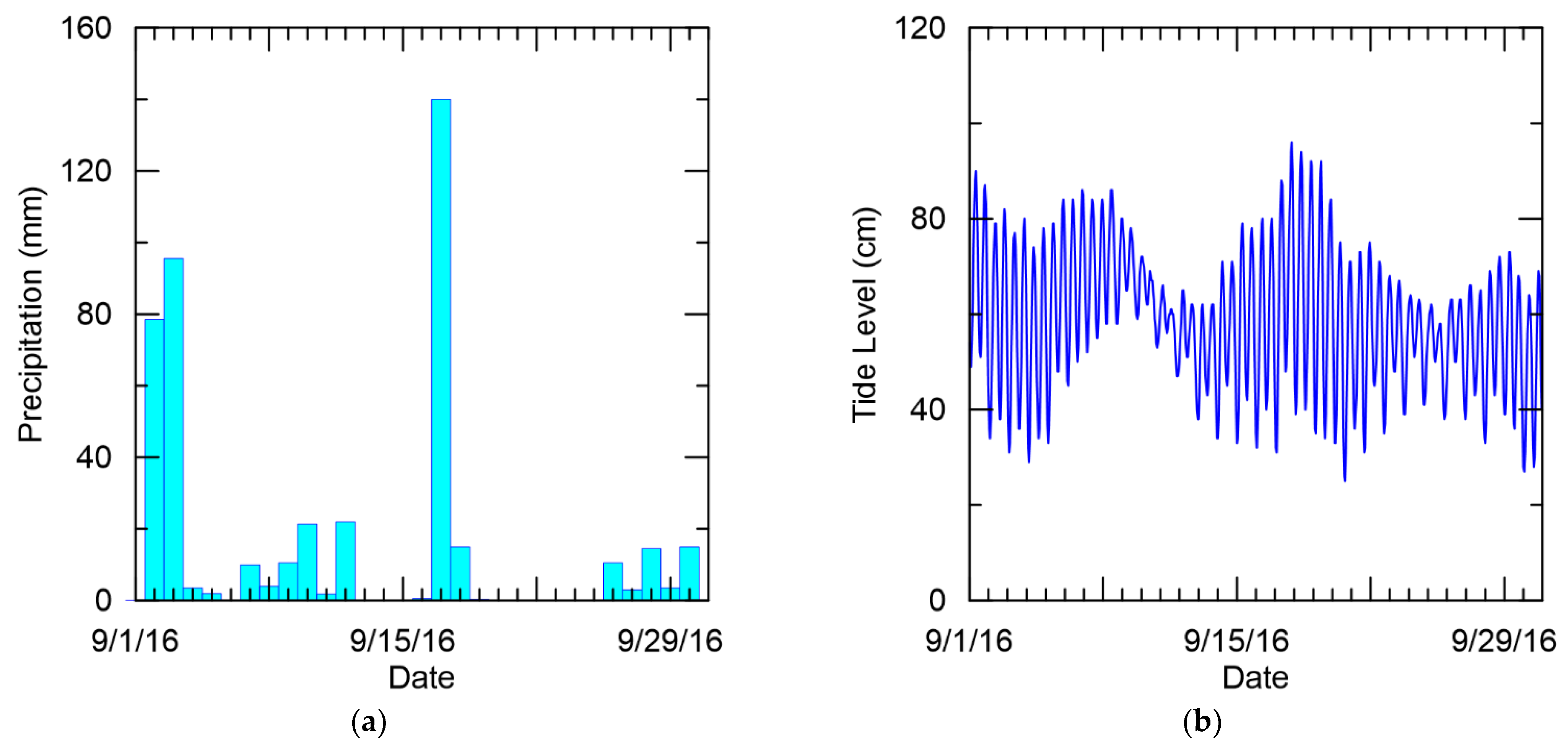
The daily precipitation levels for the month of September are shown in Figure 4a. This figure shows three small storms that delivered an estimated 80 to 95 mm of rain from 2 to 3 September, with some light showers starting around 10 September, and 140 mm on 17 September. This suggests there was some precipitation on the dates of the foreshocks and main shock. The results of the augmented Dickey–Fuller tests suggest that the precipitation data are I(0) and I(1) for both daily and hourly data resolutions with p-values < 0.01.
The daily tidal levels for the month of September are shown in Figure 4b. This figure shows the tide levels to be 30 to 90 cm above the mean sea level during the time period considered. Although the data appear to show oscillating behavior, as expected, the data do not seem to show a significant general trend in any direction. The results of the augmented Dickey–Fuller tests suggest that the tidal level data are I(1) for both daily and hourly data resolutions with p-values < 0.01.
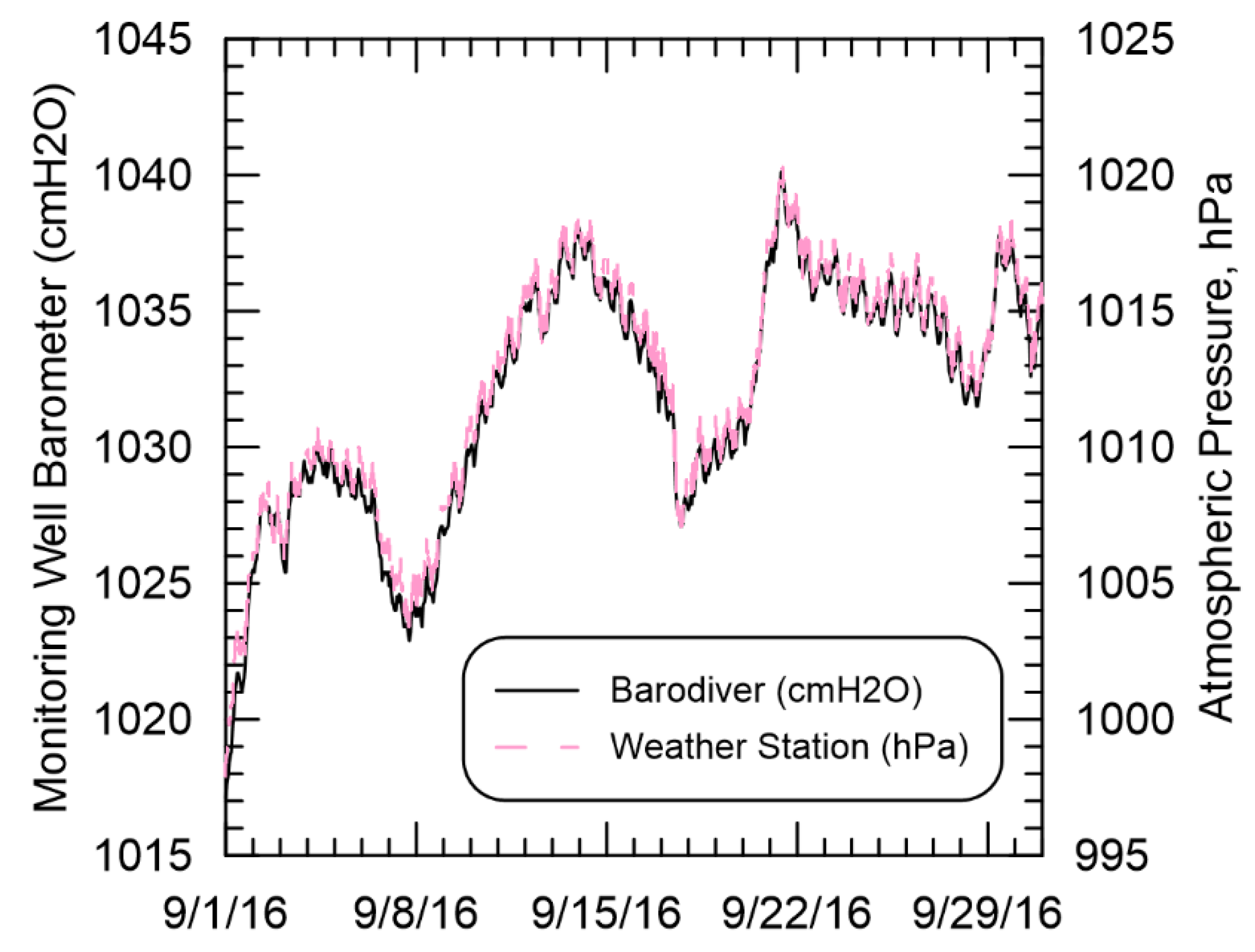
Additionally, barometric readings are shown in Figure 5. Data from the monitoring well barometer are shown alongside the data from the nearest weather station. Although these records are from two different locations, the readings are not that different.
3.2. Groundwater Monitoring Wells
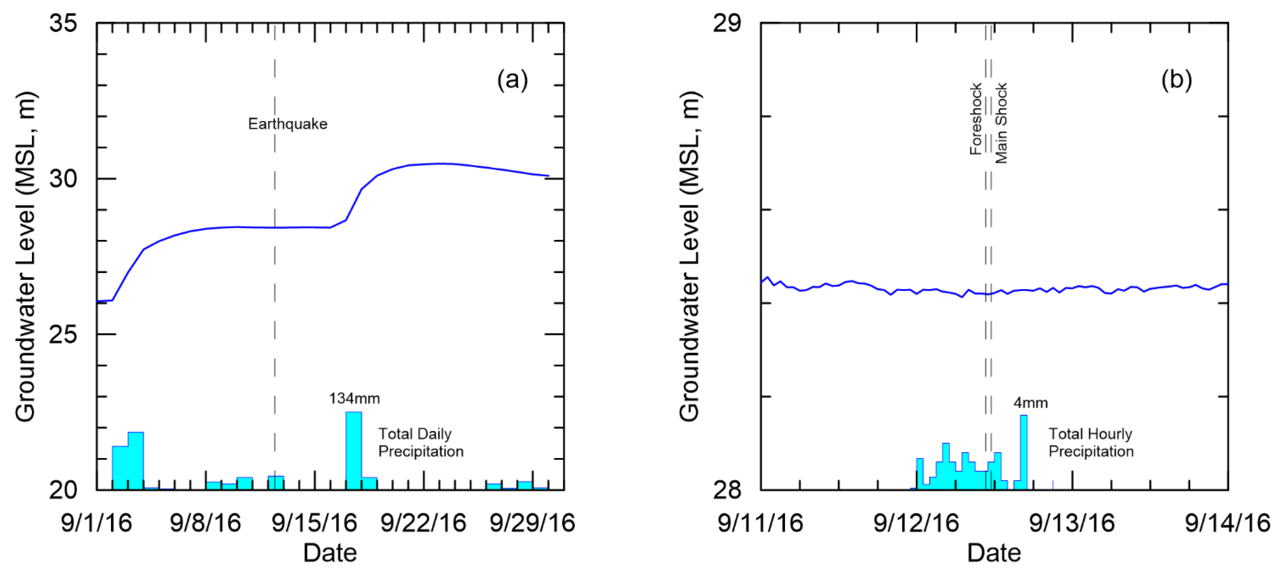
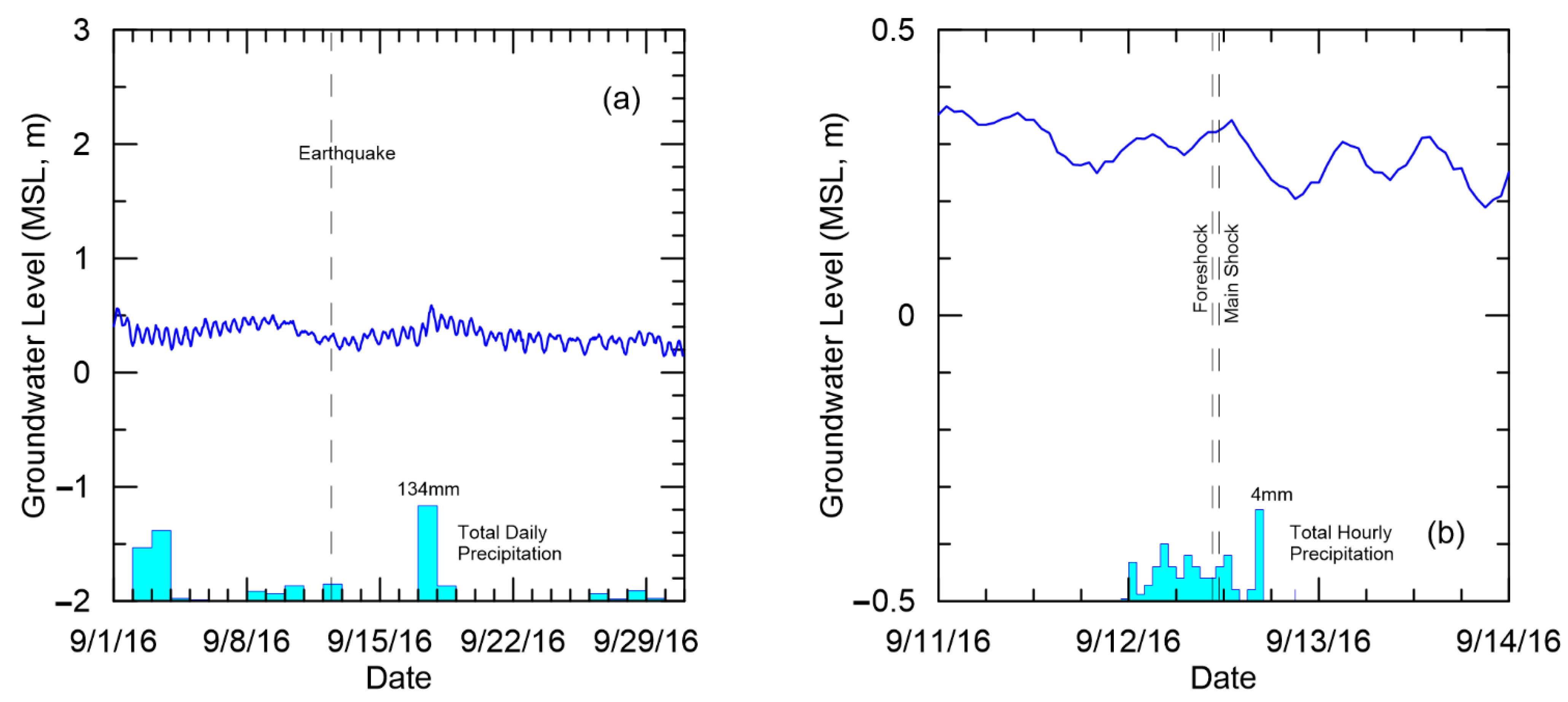
Figure 6a shows daily groundwater levels from groundwater monitoring well W1 for the month of September 2016. It shows groundwater levels to be at approximately 26 m above sea level at the beginning of September, then gradually increasing to about 28 m above sea level in about three days and staying steady for two weeks. Then, the groundwater rose again to about 30.5 m above sea level and steadily declined to 30 m above sea level at the end of September. There appears to be a groundwater offset of approximately +4 m for September. Also shown in the figure are daily precipitation levels to show when precipitation occurred. The date of the 2016 Gyeongju earthquake is also marked for reference. Figure 6b shows a closer view of the groundwater levels from 11 September to 14 September 2016. This figure suggests groundwater levels were quite steady during and around the earthquake.
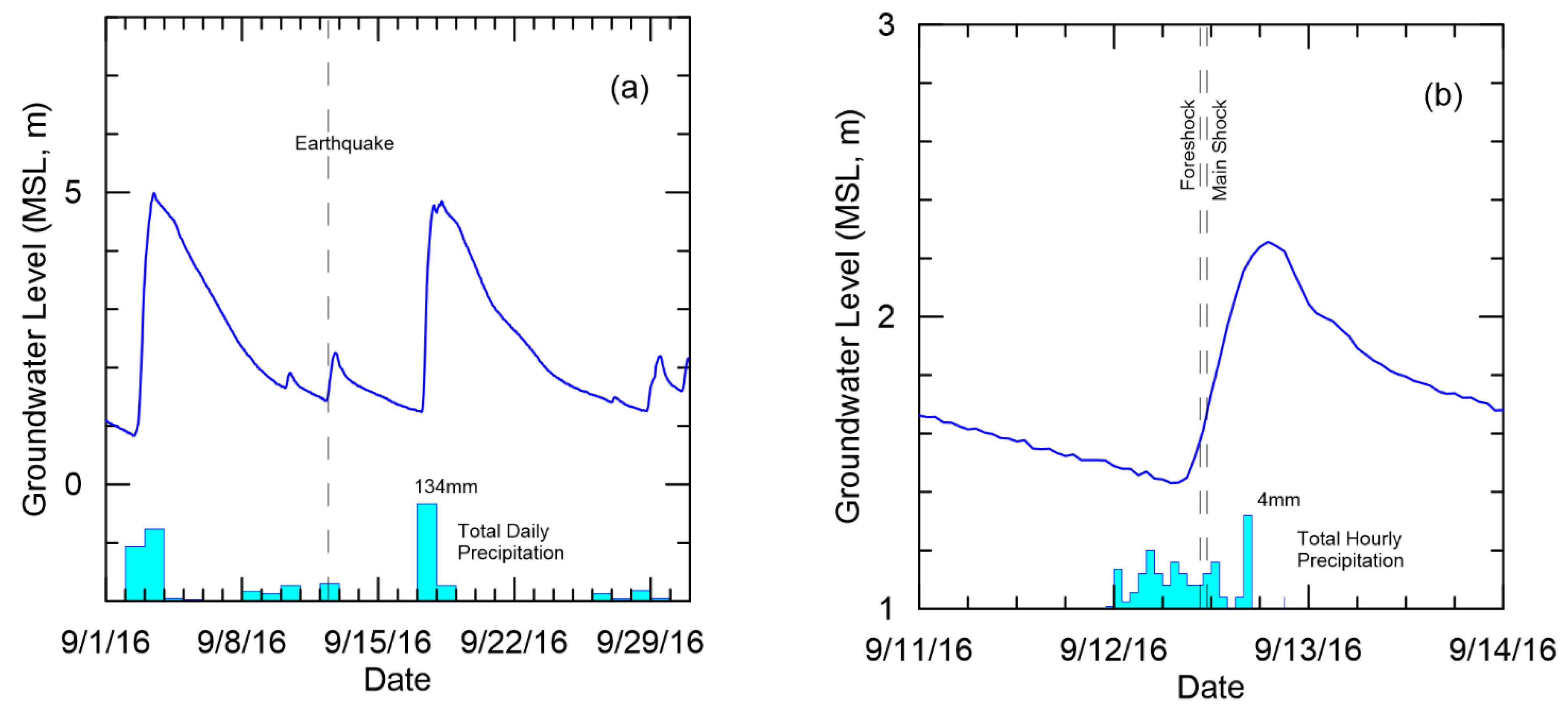
Figure 7 is in a similar format to Figure 6. Figure 7a shows daily groundwater levels from groundwater monitoring well W2 for the month of September 2016. The figure also shows several spikes in groundwater levels during September. Groundwater levels were at 1 m above sea level at the beginning of September, rising to about 5 m around 3 September, then steadily decreasing to about 1.5 m in 10 days, continuing with a few oscillations until 17 September, when it rose to 5 m above sea level. From there on, groundwater levels steadily declined to an assumed base flow of about 1 m, where it began to oscillate around 29 September. Figure 7b offers a magnified view of the groundwater levels from 11 September to 14 September 2016. This shows declining groundwater levels until the morning of 12 September 2016 and then a steep rise from 1.4 m to 2.2 m above sea level on the night of 12 September 2016. There is a gradual decline afterwards. The foreshocks and main shock occurred a little after the rise in groundwater levels began.
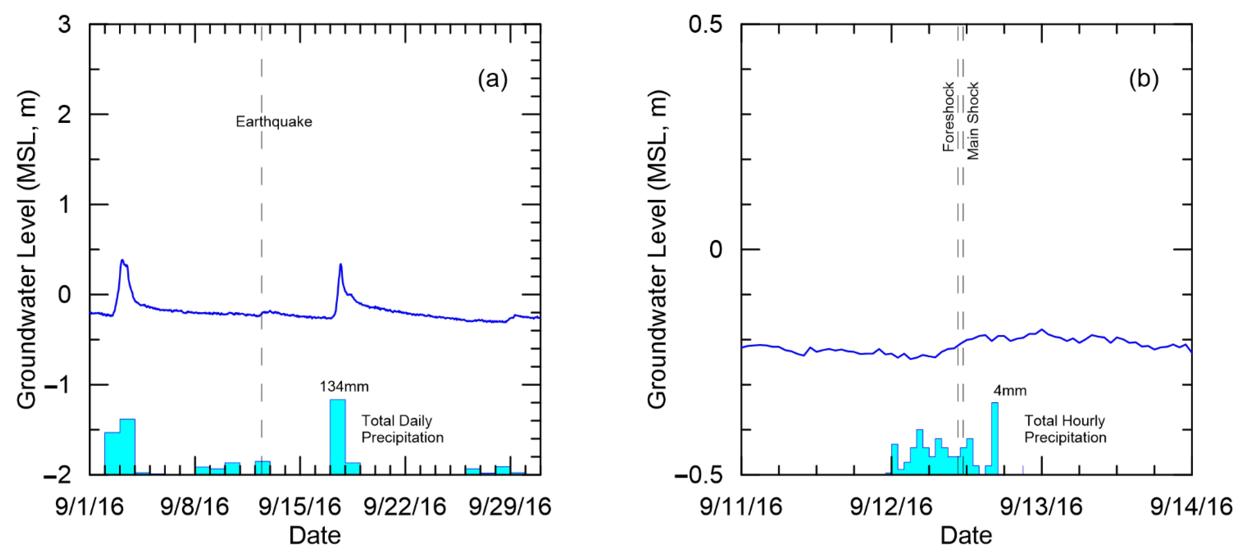
Figure 8a shows daily groundwater levels from groundwater monitoring well W3 for the month of September 2016. It shows groundwater levels to be at about 0.2 m below sea level, a slight rise to about 0.4 m above sea level two days later, then a sharp decline to an assumed base flow of about 0.4 m below sea level. There was a slight increase around 12 September which then reverted to the base flow level. Another sudden rise in groundwater levels occurred on 17 September, like the one on 3 September. Figure 8b magnifies groundwater levels around the main shock, showing more or less steady levels. Although it would not be wrong to observe that there might be a minute rise in groundwater levels from the morning to the night of 12 September, the groundwater levels around 12 September are at similar groundwater levels at other times within the figure.
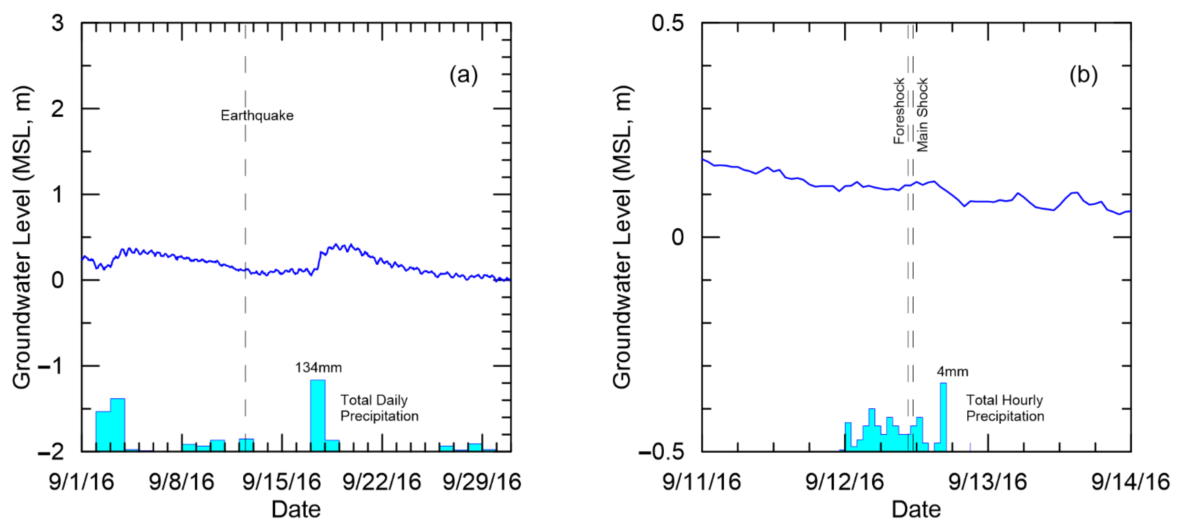
Figure 9a shows daily groundwater levels from groundwater monitoring well W4 for the month of September 2016. The groundwater level readings seem similar to those from groundwater monitoring well W3, where there is a slight increase around 3 September from about 0.1 m to about 0.3 m above sea level, and then a slow decrease to about 0.1 m over two weeks. There is another rise in groundwater levels to about 0.3 m above sea level and again a gradual and slow decline in groundwater levels over two weeks to about 0 m. Figure 9b magnifies the time around the earthquake and shows a slight drop across three days, from 0.2 m to 0.05 m above sea level.
Figure 10a shows daily groundwater levels from groundwater monitoring well W5 for the month of September 2016. This monitoring well appears to show more oscillatory behavior over the month, ranging from 0.1 m to 0.6 m above sea level, similar to the tide level data. There does not appear to be any significant discernible pattern overall. Figure 10b magnifies the groundwater levels around the time of the earthquake. It also shows oscillatory groundwater levels in the range of 0.2 m to 0.35 m above sea level, but in a slightly monotonically decreasing fashion.
Observations from groundwater monitoring wells W1 to W4 suggest that precipitation may be the cause of the rise of groundwater levels around 2 September and 17 September. Other spikes in the groundwater levels can be attributed to smaller precipitation events. None clearly indicate the Gyeongju earthquake occurred before a sudden rise in groundwater levels.
3.3. Cross-Correlation Analysis
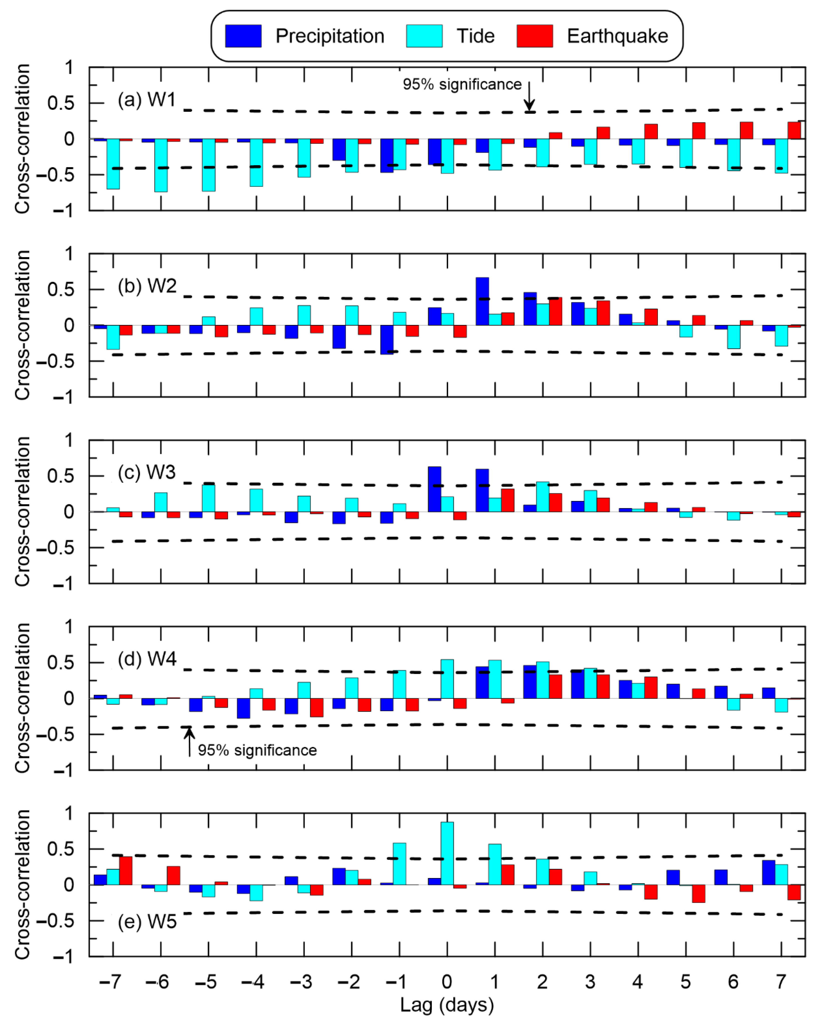
Figure 11 plots the results of the cross-correlation analyses on all groundwater monitoring wells against precipitation, tide, and earthquake. Lags are taken in days for about one week before and after the earthquake event, which in this case was on 12 September 2016. Also plotted in the figure are dotted lines denoting the minimum r for 95% significance.
Figure 11a shows the largest correlation with precipitation of approximately −0.45 at a lag of −1 day, suggesting that precipitation leads groundwater levels. Interestingly, the correlation with tide levels also does not appear too strong, except at around a lag of −4 to −7 days, also suggesting that tide levels lead groundwater levels at well W1. The correlations of groundwater levels with the series representation of the earthquake event do not appear significant. Figure 11b shows the highest correlation of about 0.7 against precipitation, which appears at a lag of 1 day, suggesting that precipitation lags groundwater level. Similar significant correlation coefficients exist at lags of 2 and −1 days. The cross-correlation results concerning tide levels and the earthquake did not show significant correlations across lags at well W2. Like well W2, Figure 10c shows well W3 to have the highest correlation of about 0.6 against precipitation at a lag of 0 and 1 days, with a majority of the lags having a correlation of about ±0.2. The cross-correlation results concerning the tide levels reached a maximum of about 0.4 at 2 days, while the earthquake did not show significant correlations across lags. For well W4, Figure 10d shows a correlation of about 0.5 at a lag of 0 and 1 days for tide levels. This might not be surprising, as groundwater monitoring well W4 is closer to the ocean than well W3. The cross-correlation with precipitation shows results within ±0.4, while the main shock shows results within ±0.3. Figure 10e does not show a strong correlation with precipitation at well W5, with the highest correlation of about −0.35 at a lag of 7 days. Similarly, the correlations with the earthquake also appear to be limited to within ±0.4. Interestingly, the correlation with tide levels appears to show the highest correlation of all wells, close to 0.9 at a lag of 0 days. Other than the tide, there does not appear to be much correlation at any lag. These results suggest that wells W1, W4, and W5 show some relationship with tide levels, where well W1 seems to suggest that increases in tide levels occur first and then a corresponding decrease in groundwater levels occurs 4 to 7 days later, while wells W4 and W5 suggest a simultaneous increase. Wells W3 and W4 suggest that groundwater levels increase about 0 to 1 days after a precipitation event.
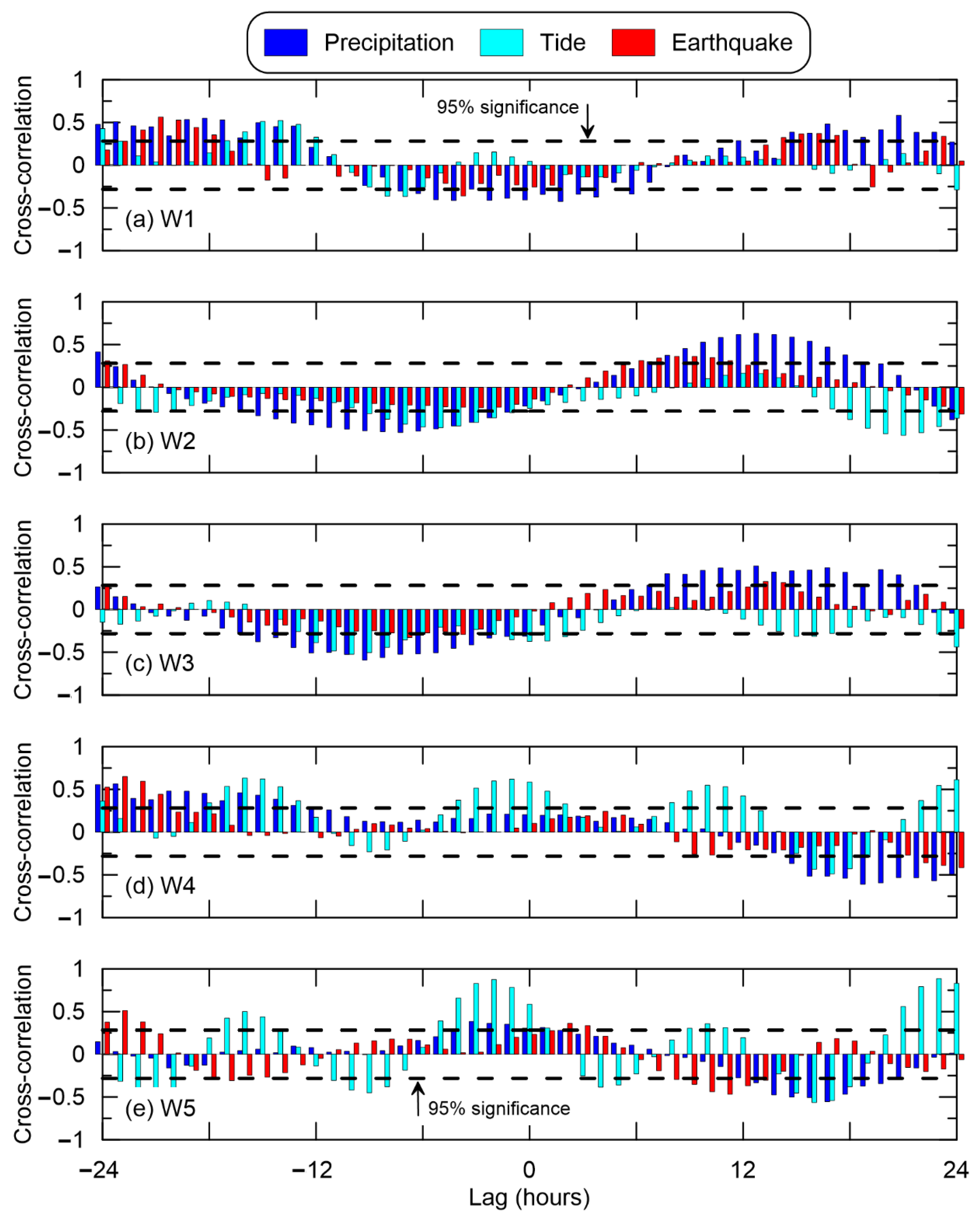
Figure 12 plots the results of the cross-correlation analyses with the lag being taken as hourly with a window spanning one day before and after the earthquake event. Again, the black dotted lines denote the minimum r for 95% significance. These limits are different due to the shorter time period of interest.
These results for well W1, as plotted in Figure 12a, show precipitation to be statistically significant several hours within the earthquake event as well as approximately 18 h before and after the event, suggesting that precipitation both leads and lags groundwater levels. However, the signs of the correlation coefficients suggest that rain events around 12 September, 11:00 UTC, are correlated with a drop in groundwater levels, while rain events 1.5 days before and after 12 September, 11:00 UTC could be correlated with a rise in groundwater levels. Additionally, the tide does not show as strong of a correlation with groundwater levels at this resolution and time period, relative to Figure 11a. Surprisingly, the figure shows a significant correlation between the earthquake at −4 and −20 and −21 h, suggesting that the earthquake is correlated to an initial drop in groundwater levels 4 h later or possibly a rise in groundwater levels about 20 h later. Interestingly, none of these instances seem to appear in Figure 6. For wells W2 and W3, the analysis of precipitation shows significant negative correlation coefficients from −1 to −15 h of lag as well as significant positive correlation coefficients from 7 to 21 lag hours. What is interesting is that after −15 and 21 lag hours, the correlation coefficients become positive. Correlations with the tide are also similar, although well W2 seems to deem tide as relatively more significant than well W3. Both wells seem to show a few correlations with the earthquake at the 95% limit on different lags, such as lags 17 to 20 for well W2 and lag 13 and 14 as well as −4 to −7 for well W3. Note that well W3 does not appear to show any major groundwater fluctuation around the time of the earthquake. Wells W4 and W5 appear to show similar and significant correlations for tide. These two wells are closest to the shoreline. Additionally, both wells show similar and significant correlations for precipitation, although well W4 shows several statistically significant correlations at lags of less than −14 h. Interestingly, statistically significant correlations exist at lags of ±22 or greater hours for well W4, while statistically significant correlations exist at lags of −22 h or less for well W5. There are also scattered correlations at 2 to 3 and 9 to 12 lag hours for well W5. Note that both wells W4 and W5 exhibited a consistent undulating groundwater level profile around the time of the earthquakes. These results are in line with the interpretation derived from Figure 11.
Overall, the cross-correlation analyses suggest that wells W2 and W3 exhibited similar behavior tied to precipitation while wells W4 and W5 exhibited similar behavior closely tied to tides. Hourly correlations for wells W1, W2, and W3 showed similar correlations with precipitation and earthquake, although some of the correlations with precipitation were statistically significant while a majority of those correlations with the earthquake were not statistically significant. Additionally, both wells W4 and W5 suggest that the earthquake leads groundwater levels by about one day. Note that although there are statistically significant correlations in well W1, the groundwater levels as shown in Figure 6b appear relatively stable and flat.
3.4. Granger Causality Tests
The results from the augmented Dickey–Fuller test are shown in Table 1 for wells W1 through W5. The data window being tested is one day before and after the main shock. The table shows that all wells are at least I(1), which suggests that the groundwater level data are stationary and satisfy the condition for the Granger causality test. As a side note, all wells showed stationarity with I(1) when all the data for September were considered.
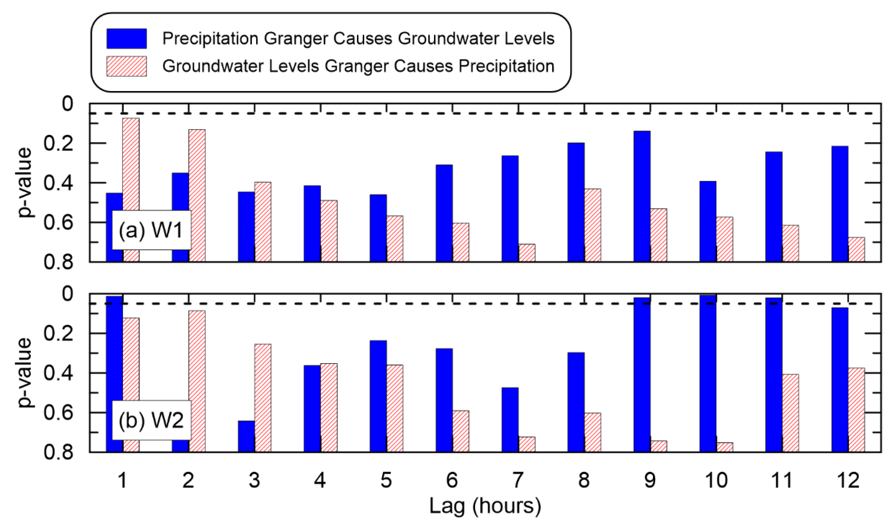
The partial Granger causality test results involving precipitation are shown in Figure 13. Results in the form of p-values per lag are displayed with a dotted line indicating α = 0.05. Bars with portions above this dotted line indicate statistical significance. Only wells W1 and W2 are presented due to brevity and redundancy. Well W1 does not have any p-values of statistical significance, suggesting that precipitation does not Granger-cause groundwater levels and vice versa. Wells W4 and W5 also did not show Granger causality with precipitation across the lags considered. However, well W2 shows statistically significant p-values at lags of 1 and 9 through 11, suggesting that precipitation Granger-causes groundwater levels at W2. The figure also suggests that the opposite, that groundwater levels Granger-cause precipitation, is not true. Results for well W3 are similar to W2. It should be noted that when all the data for the month of September were processed, it was shown that precipitation Granger-causes groundwater levels for wells W1 through W4, but also that groundwater levels Granger-cause precipitation at all wells.
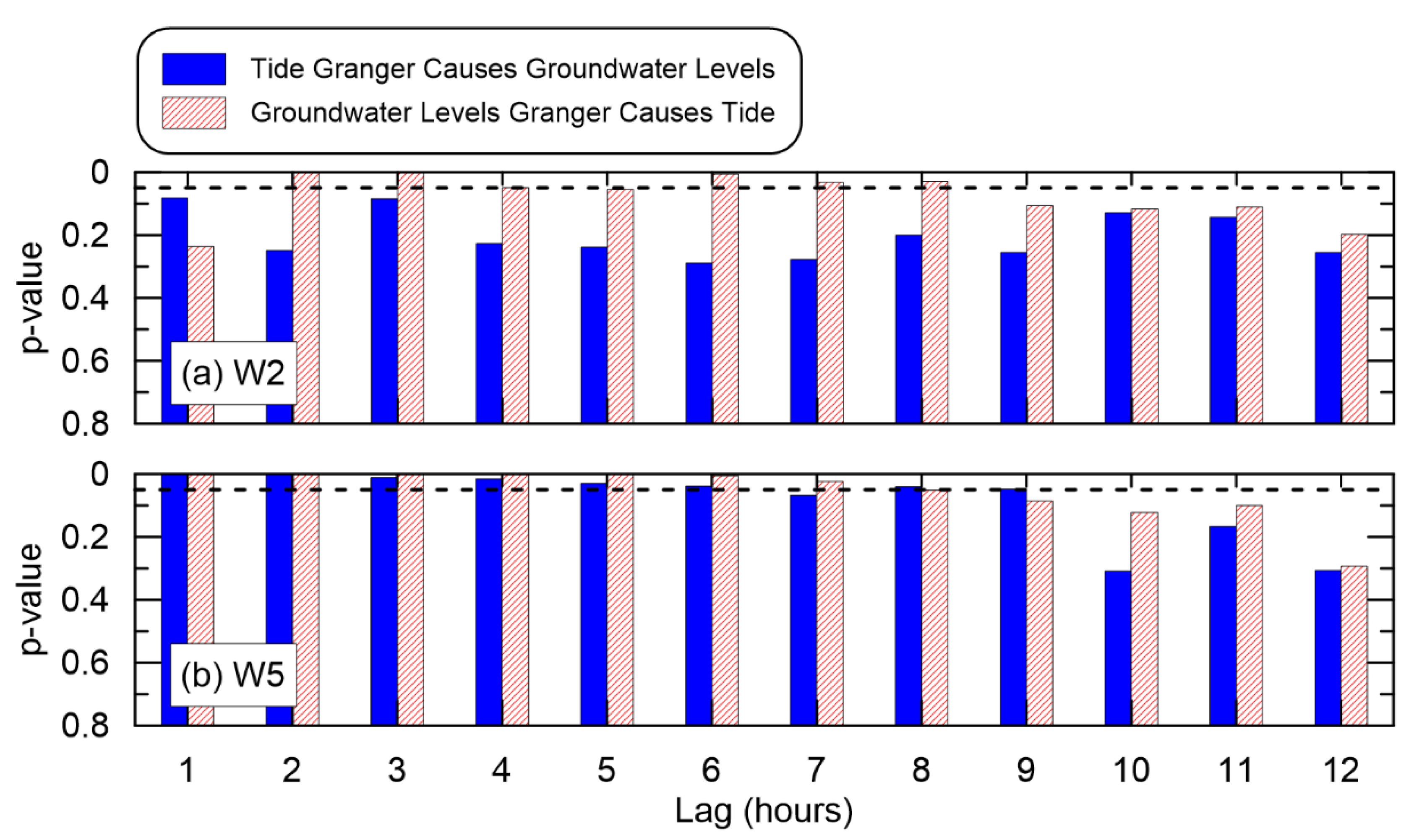
Figure 14 presents Granger causality test results for groundwater levels and tide for wells W2 and W5. Results for well W2 suggest that tide does not Granger-cause groundwater levels. However, the results do suggest that groundwater levels Granger-cause tide at multiple lags. Wells W1 and W3 also suggested similar Granger causality. Well W5 suggests that both tide Granger-causes groundwater levels and groundwater levels Granger-cause tide, especially at earlier lags. Results for well W4 are similar to W5. It should be noted that when all the data for the month of September were processed, all wells suggested that tide Granger-causes groundwater levels and vice versa.
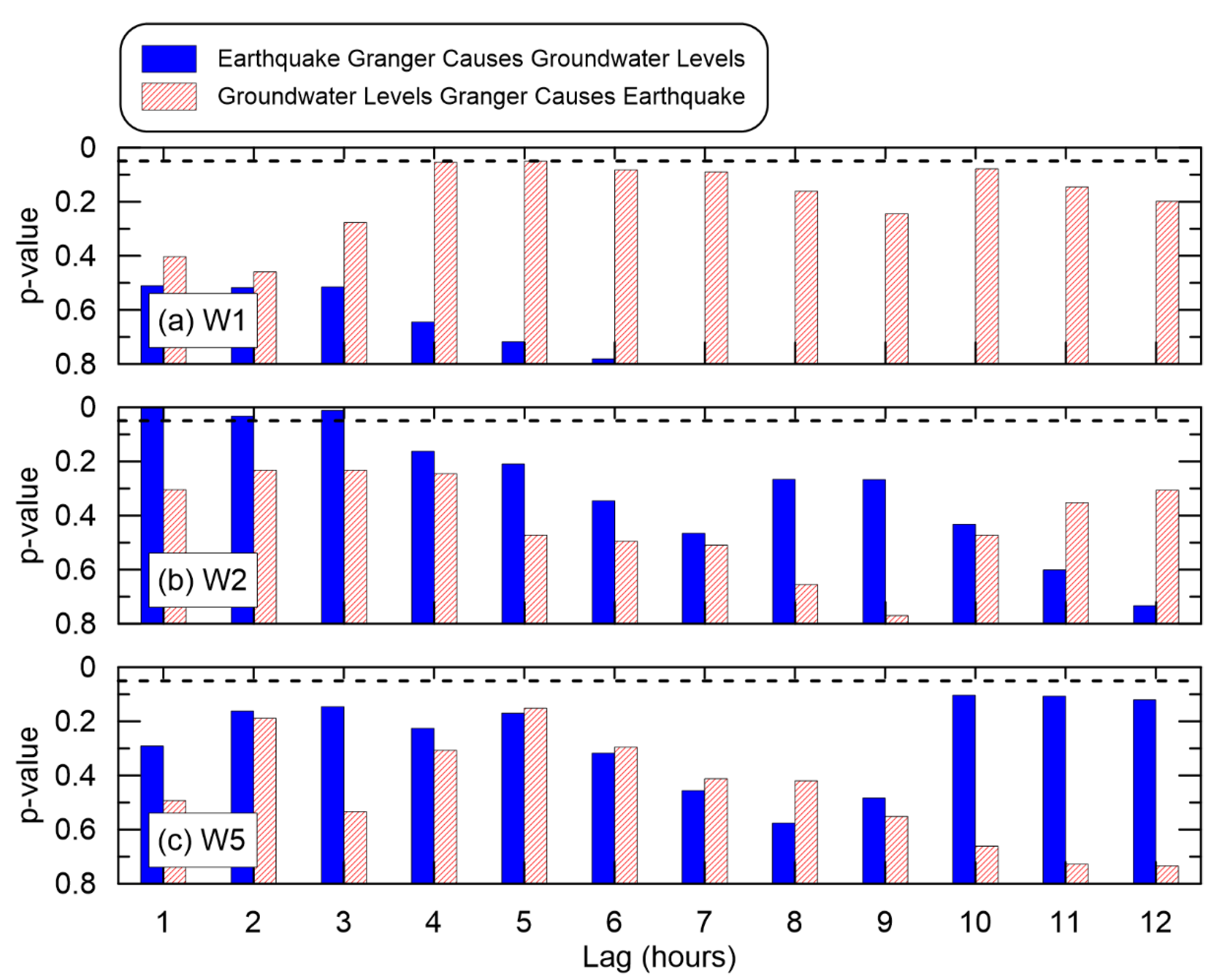
Granger causality test results involving the earthquake are shown in Figure 15 for wells W1, W2, and W5. Not surprisingly, the test provided no statistically significant results at the lags investigated for well W1. However, at smaller lags, well W2 suggests that earthquake Granger-causes groundwater levels. Strangely enough, well W3 did not show that earthquake Granger-causes groundwater levels even though the groundwater level patterns are similar to well W2. Both wells W4 and W5 did not show statistical significance at the lags investigated with well W5. When all data in the month of September were considered, wells W1 and W2 suggested that earthquake Granger-causes groundwater levels and that groundwater levels Granger-cause earthquakes in well W1.
4. Discussion
Overall, it appears the earthquake affected groundwater levels at well W2 only. This is in agreement with the observed groundwater levels but does not preclude precipitation effects. It is unsure why well W3 did not show similar Granger causality test results given the similar groundwater level patterns. Hydrologically speaking, precipitation along with infiltration should have a strong impact on groundwater levels, but the Granger causality test did not suggest so for wells W1, W4, and W5. In agreement with the observed groundwater levels at wells W4 and W5, the Granger causality test also showed a positive influence both ways when all the available data were considered, suggesting a Type 2 error. This does bring up an issue with such complex statistical techniques, where bias and variability are minimized, but an interpretation is required. In this case, there is no hydrological mechanism where groundwater levels would lead to precipitation. A far-fetched interpretation would be that some form of extreme evaporation led to sudden condensation in the local atmosphere. The authors would like the reader to understand that this interpretation is highly improbable and should not be considered. This leads to the user having a certain mastery of the problems at hand to provide a reasonable interpretation of the results from such advanced statistical techniques. For example, as shown previously in the analyses, varying numbers of data can lead to different results, which forces the user to consider how many data are appropriate. Not enough data leads to Type 1 errors while too many data can lead to Type 2 errors.
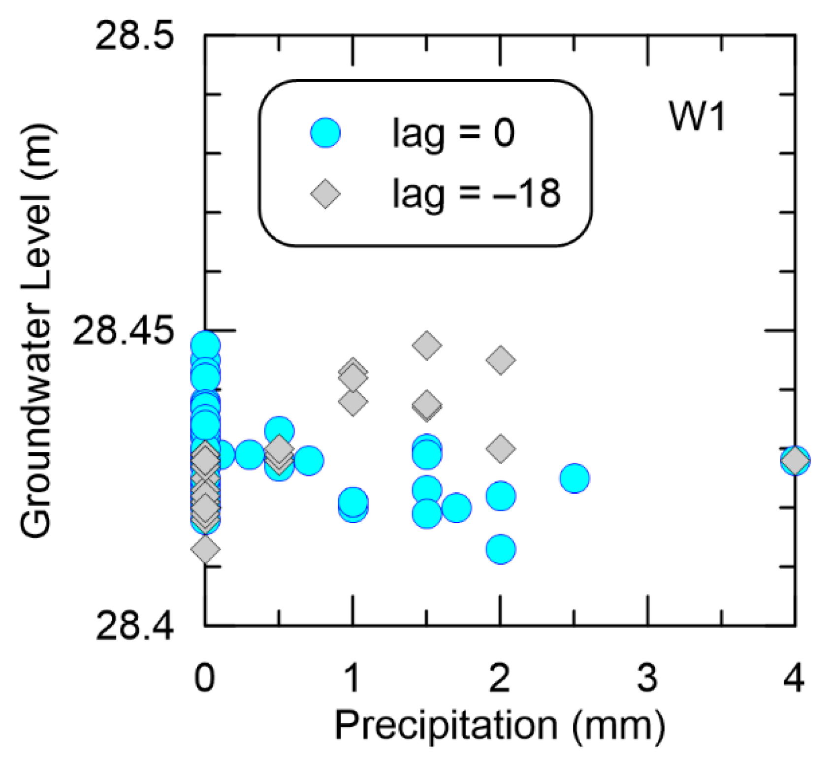
What is interesting is that both Granger causality testing and cross-correlation analyses yielded statistically significant results at lower lags. This is especially true for precipitation with respect to wells W2 and W3 and with respect to tide for wells W4 and W5. Although visually, it would appear that the groundwater level increases in well W1 most likely resulted from large precipitation events, this did not show up in the Granger causality tests, but as a negative correlation coefficient in cross-correlation analysis. These negative correlation coefficients appear at multiple lags across different wells, implying that an increase in precipitation is correlated with a decrease in groundwater levels. Figure 16 plots precipitation versus groundwater levels for well W1 at lag = 0. This shows a negative correlation, as most of the data are at a precipitation of 0 mm. Shifting the data to give lag = −18 changes the correlation to a positive value. This suggests that cross-correlation analyses should be carefully utilized, especially when one value is frequent, such as 0 mm for precipitation events and a magnitude of 0 for earthquake events.
In terms of earthquake forecasting, Granger causality testing did not yield any statistically significant results in this case, i.e., groundwater levels Granger-cause earthquakes. For cross-correlation analyses, the forecasting would have shown statistically significant correlations when “groundwater levels lead earthquake”, which would occur on the opposite side of “earthquake leads groundwater levels”. These would be positive lags in Figure 11 and Figure 12. Well W1 shows significant positive correlations at 14 to 17 lag hours, well W2 shows significant positive correlations at 6 to 10 lag hours, and well W3 shows significant positive correlations at 13 to 14 lag hours. However, there were no significant results from wells W4 and W5, which seemed more sensitive to the tide. There were no statistically significant correlations with the earthquake using the daily lags, demonstrating the importance of data resolution for cross-correlation analyses. This is in agreement with some of the conclusions in previous studies [24,25].
However, there may be an issue that the earthquake was not strong enough to trigger a groundwater response. A more recent relationship describing at what distance earthquake precursory changes can be observed is [27,43]:
where r = radius in km and M = earthquake magnitude. For this study, r = 231 km. This is larger than the 27 km distance from the epicenter to the power plant.
Additionally, there did not appear to be strong qualitative and quantitative evidence of groundwater level changes in the days leading up to the earthquake, with both the largest foreshock and the main shock occurring within an hour of each other. Moreover, groundwater monitoring well data show that each well took several days to dissipate hydraulic head to base flow levels, suggesting that any evident increase or decrease most likely would have lasted several days, especially when considering that precipitation records did not show any storms lasting for an equivalent time period.
5. Conclusions
To ascertain if groundwater levels at a plant site were affected by the 2016 Gyeongju earthquake, qualitative and quantitative methods were applied. An examination of the groundwater levels at five groundwater monitoring wells scattered across a plant site indicated that there was no significant increase or decrease in groundwater levels on the same day or a few days afterwards. Additionally, there were no noticeable groundwater level changes in the days leading up to an earthquake for earthquake forecasting purposes. Cross-correlation analyses suggested tide to show some lag in three of the five groundwater monitoring wells, while precipitation showed a moderate correlation in the remaining two groundwater monitoring wells. Indirect evidence, through population reports on ground shaking as well as median estimates of expected ground shaking, suggests the earthquake to have induced little to moderate levels of straining on the ground at the plant site.
Author Contributions
Conceptualization, E.Y.; methodology, E.Y.; software, E.Y.; formal analysis, E.Y.; investigation, M.C.; resources, M.C.; writing—original draft preparation, E.Y.; writing—review and editing, E.Y.; visualization, E.Y.; supervision, E.Y.; project administration, E.Y.; funding acquisition, E.Y. All authors have read and agreed to the published version of the manuscript.
Funding
This work was supported by the 2022 Research Fund of the KEPCO International Nuclear Graduate School (KINGS), Republic of Korea.
Institutional Review Board Statement
Not applicable.
Informed Consent Statement
Not applicable.
Data Availability Statement
Publicly available datasets were analyzed in this study. Any generated data can be found within this article.
Conflicts of Interest
The authors declare no conflict of interest.
References
- Baba, A.; Kaya, A.; Birsoy, Y. The effect of yatagan thermal power plant (mugla, turkey) on the quality of surface and ground waters. Water Air Soil Pollut. 2003, 149, 93–111. [Google Scholar] [CrossRef]
- Pandey, V.; Ray, M.; Kumar, V. Assessment of water-quality parameters of groundwater contaminated by fly ash leachate near Koradi Thermal Power Plant, Nagpur. Environ. Sci. Pollut. Res. 2020, 27, 27422–27434. [Google Scholar] [CrossRef]
- Zhao, Y.Y.; Zhang, Y.; Liu, X.C.; Wang, J. Prediction of groundwater environmental impact on a power plant under accident conditions. Environ. Earth Sci. 2018, 77, 522. [Google Scholar] [CrossRef]
- Eldardiry, H.; Habib, E. Carbon capture and sequestration in power generation: Review of impacts and opportunities for water sustainability. Energy Sustain. Soc. 2018, 8, 6. [Google Scholar] [CrossRef] [Green Version]
- Park, J.B.; Jung, H.R.; Lee, E.Y.; Kim, C.L.; Kim, G.Y.; Kim, K.S.; Koh, Y.K.; Park, K.W.; Cheong, J.H.; Jeong, C.W.; et al. Wolsong low- and intermediate-level radioactive waste disposal center: Progress and challenges. Nucl. Eng. Technol. 2009, 41, 477–492. [Google Scholar] [CrossRef] [Green Version]
- Liu, L.-B.; Roeloffs, E.; Zheng, X.-Y. Seismically induced water level fluctuations in the Wali well, Beijing, China. J. Geophys. Res. 1989, 94, 9453–9462. [Google Scholar] [CrossRef]
- Ohno, M.; Wakita, H.; Kanjo, K. A water well sensitive to seismic waves. Geophys. Res. Lett. 1997, 24, 691–694. [Google Scholar] [CrossRef]
- Muir-Wood, R.; King, G.C.P. Hydrological signatures of earthquake strain. J. Geophys. Res. Solid Earth 1993, 98, 22035–22068. [Google Scholar] [CrossRef]
- Roeloffs, E. Poroelastic techniques in the study of earthquake-related hydrologic phenomena. Adv. Geophys. 1996, 37, 135–195. [Google Scholar] [CrossRef]
- Wang, H.F. Effects of deviatoric stress on undrained pore pressure response to fault slip. J. Geophys. Res. Solid Earth 1997, 102, 17943–17950. [Google Scholar] [CrossRef]
- Domenico, P.A.; Schwartz, F.W. Physical and Chemical Hydrogeology, 2nd ed.; Wiley and Sons: New York, NY, USA, 1998; pp. 1–528. [Google Scholar]
- Cooper, H.H., Jr.; Bredehoeft, J.D.; Papadopulos, I.S.; Bennett, R.R. The response of well-aquifer systems to seismic waves. J. Geophys. Res. 1965, 70, 3915–3926. [Google Scholar] [CrossRef]
- Brodsky, E.E.; Roeloffs, E.; Woodcock, D.; Gall, I.; Manga, M. A mechanism for sustained groundwater pressure changes induced by distant earthquakes. J. Geophys. Res. 2003, 108, 1–10. [Google Scholar] [CrossRef] [Green Version]
- Cleasson, L.; Skelton, A.; Graham, C.; Morth, C.M. The timescale and mechanisms of fault sealing and water–rock interaction after an earthquake. Geofluids 2007, 7, 427–440. [Google Scholar] [CrossRef]
- Jang, C.S.; Liu, C.W.; Chia, Y.; Cheng, L.H.; Chen, Y.C. Changes in hydrogeological properties of the River Choushui alluvial fan aquifer due to the 1999 Chi-Chi earthquake, Taiwan. Hydrogeol. J. 2008, 16, 389–397. [Google Scholar] [CrossRef]
- M 5.4–6 km S of Gyeongju, South Korea. Available online: https://earthquake.usgs.gov/earthquakes/eventpage/us10006p1f/executive (accessed on 6 May 2022).
- Uchide, T.H.; Song, S.G. Fault rupture model of the 2016 gyeongju, south korea, earthquake and its implication for the underground fault system. Geophys. Res. Lett. 2018, 45, 2257–2264. [Google Scholar] [CrossRef]
- Woo, J.U.; Rhie, J.K.; Kim, S.R.; Kang, T.S.; Kim, K.H.; Kim, Y.H. The 2016 gyeongju earthquake sequence revisited: Aftershock interactions within a complex fault system. Geophys. J. Int. 2019, 217, 58–74. [Google Scholar] [CrossRef] [Green Version]
- M 4.9–14 km SW of Gyeongju, South Korea. Available online: https://earthquake.usgs.gov/earthquakes/eventpage/us10006p12/executive (accessed on 6 May 2022).
- Davison, C. On scales of seismic intensity and on the construction and use of isoseismal lines. Bull. Seismol. Soc. Am. 1921, 11, 95–129. [Google Scholar] [CrossRef]
- Wood, H.O.; Neumann, F. Modified Mercalli Intensity Scale of 1931. Bull. Seismol. Soc. Am. 1931, 21, 277–283. [Google Scholar] [CrossRef]
- The National Atlas of Korea. Available online: http://nationalatlas.ngii.go.kr/pages/page_1288.php (accessed on 6 May 2022).
- Kim, G.B.; Choi, M.R.; Lee, C.J.; Shin, S.H.; Kim, H.J. Characteristics of spatio-temporal distribution of groundwater level’s change after 2016 gyeongju earthquake. J. Geol. Soc. Korea 2018, 54, 93–105. [Google Scholar] [CrossRef]
- Lee, J.Y. Gyeongju earthquakes recorded in daily groundwater data at national groundwater monitoring stations in gyeongju. J. Soil Groundw. Environ. 2016, 21, 80–86. [Google Scholar] [CrossRef]
- Lee, J.W.; Woo, N.C.; Koh, D.-C.; Kim, K.-Y.; Ko, K.-S. Assessing aquifer responses to earthquakes using temporal variations in groundwater monitoring data in alluvial and sedimentary bedrock aquifers. Geomat. Nat. Hazards Risk 2020, 11, 742–765. [Google Scholar] [CrossRef]
- Lee, H.A.; Hamm, S.Y.; Woo, N.C. The abnormal groundwater changes as potential precursors of 2016 ml 5.8 gyeongju earthquake in korea. Econ. Environ. Geol. 2018, 51, 393–400. [Google Scholar] [CrossRef]
- Lee, H.A.; Hamm, S.Y.; Woo, N.C. Pilot-scale groundwater monitoring network for earthquake surveillance and forecasting research in korea. Water 2021, 13, 2448. [Google Scholar] [CrossRef]
- Wallace, R.E.; Teng, T.-L. Prediction of the Sungpan-Pingwu earthquakes, August 1976. Bull. Seismol. Soc. Am. 1980, 70, 1199–1223. [Google Scholar] [CrossRef]
- Merifield, P.; Lamar, D. Possible strain events reflected in water levels in wells along San Jacinto fault zone, southern California. Pure Appl. Geophys. 1984, 122, 245–254. [Google Scholar] [CrossRef]
- Martinelli, G. Contributions to a history of earthquake prediction research. Seismol. Res. Lett. 2000, 71, 583–588. [Google Scholar] [CrossRef]
- Song, S.-R.; Ku, W.-Y.; Chen, Y.-L.; Lin, Y.-C.; Liu, C.-M.; Kuo, L.-W.; Yang, T.F.; Lo, H.-J. Groundwater chemical anomaly before and after the Chi-Chi earthquake in Taiwan. Terr. Atmos. Ocean. Sci. 2003, 14, 311–320. [Google Scholar] [CrossRef] [Green Version]
- Huang, F.; Li, M.; Ma, Y.; Han, Y.; Tian, L.; Yan, W.; Li, X. Studies on earthquake precursors in China: A review for recent 50 years. Geod. Geodyn. 2017, 8, 1–12. [Google Scholar] [CrossRef]
- Senthilkumar, M.; Gnanasundar, D.; Mohapatra, B.; Jain, A.K.; Nagar, A.; Parchure, P.K. Earthquake prediction from high frequency groundwater level data: A case study from Gujarat, India. HydroResearch 2020, 3, 118–123. [Google Scholar] [CrossRef]
- Rikitake, T. Earthquake precursors. Bull. Seismol. Soc. Am. 1975, 65, 1133–1162. [Google Scholar] [CrossRef]
- Cicerone, R.D.; Ebel, J.E.; Britton, J. A systematic compilation of earthquake precursors. Tectonophysics 2009, 476, 371–396. [Google Scholar] [CrossRef]
- Korea Meteorological Administration. Available online: http://www.kma.go.kr (accessed on 6 May 2022).
- Korea Hydrographic and Oceanographic Agency. Available online: http://www.khoa.go.kr/ (accessed on 6 May 2022).
- Granger, C.W.J. Investigating causal relations by econometric models and cross-spectral methods. Econometrica 1969, 37, 424–438. [Google Scholar] [CrossRef]
- Granger, C.W.J. Testing for causality: A personal viewpoint. J. Econ. Dyn. Control 1980, 2, 329–352. [Google Scholar] [CrossRef]
- Stokes, P.A.; Purdon, P.L. A study of problems encountered in granger causality analysis from a neuroscience perspective. Proc. Natl. Acad. Sci. USA 2017, 114, E7063–E7072. [Google Scholar] [CrossRef] [PubMed] [Green Version]
- Dickey, D.A.; Fuller, W.A. Distribution of the estimators for autoregressive time series with a unit root. J. Am. Stat. Assoc. 1979, 74, 427–431. [Google Scholar] [CrossRef]
- Fuller, W.A. Introduction to Statistical Time Series; John Wiley and Sons: New York, NY, USA, 1976. [Google Scholar]
- Dobrovolsky, I.P.; Zubkov, S.I.; Miachkin, V.I. Estimation of the size of earthquake preparation zones. Pure Appl. Geophys. 1979, 117, 1025–1044. [Google Scholar] [CrossRef]
Figure 1.
Map of South Korea showing locations of major thermal and nuclear power plant sites as well as the Wolseong Low and Intermediate Level Radioactive Waste Disposal Center. The 2016 Gyeongju earthquake epicenter is also shown, along with MMI earthquake intensity contours. Recreated and modified from [16,22].

Figure 2.
Map showing the 2016 Gyeongju earthquake epicenter and the nearby power plant study site. The inset shows the locations of five groundwater observation wells within the power plant site.
Figure 2.
Map showing the 2016 Gyeongju earthquake epicenter and the nearby power plant study site. The inset shows the locations of five groundwater observation wells within the power plant site.

Figure 3.
Example demonstrating how cross-correlation would look like for different series. The top part plots y1 = 2cos(x), y2 = 5cos(x) + 0.5, and y3 = 5cos(x − 45) + 0.5. The bottom part shows the results from the cross-correlation analysis.
Figure 3.
Example demonstrating how cross-correlation would look like for different series. The top part plots y1 = 2cos(x), y2 = 5cos(x) + 0.5, and y3 = 5cos(x − 45) + 0.5. The bottom part shows the results from the cross-correlation analysis.

Figure 4.
(a) Precipitation in Gyeongju and (b) tide levels in nearby Ulsan for the month of September 2016.
Figure 4.
(a) Precipitation in Gyeongju and (b) tide levels in nearby Ulsan for the month of September 2016.

Figure 5.
Atmospheric pressure recordings for the month of September 2016 from a monitoring well barometer as well as the nearest weather station.
Figure 5.
Atmospheric pressure recordings for the month of September 2016 from a monitoring well barometer as well as the nearest weather station.

Figure 6.
Groundwater level changes for well W1 during (a) September 2016 and (b) a closer inspection of the 3 days around the earthquake event.
Figure 6.
Groundwater level changes for well W1 during (a) September 2016 and (b) a closer inspection of the 3 days around the earthquake event.

Figure 7.
Groundwater level changes for well W2 during (a) September 2016 and (b) a closer inspection of the 3 days around the earthquake event.
Figure 7.
Groundwater level changes for well W2 during (a) September 2016 and (b) a closer inspection of the 3 days around the earthquake event.

Figure 8.
Groundwater level changes for well W3 during (a) September 2016 and (b) a closer inspection of the 3 days around the earthquake event.
Figure 8.
Groundwater level changes for well W3 during (a) September 2016 and (b) a closer inspection of the 3 days around the earthquake event.

Figure 9.
Groundwater level changes for well W4 during (a) September 2016 and (b) a closer inspection of the 3 days around the earthquake event.
Figure 9.
Groundwater level changes for well W4 during (a) September 2016 and (b) a closer inspection of the 3 days around the earthquake event.

Figure 10.
Groundwater level changes for well W5 during (a) September 2016 and (b) a closer inspection of the 3 days around the earthquake event.
Figure 10.
Groundwater level changes for well W5 during (a) September 2016 and (b) a closer inspection of the 3 days around the earthquake event.

Figure 11.
Cross-correlation analysis between groundwater levels in wells (a) W1, (b) W2, (c) W3, (d) W4, and (e) W5 against precipitation, tide, and earthquake, showing lag in days at 1 week before and after the main shock.
Figure 11.
Cross-correlation analysis between groundwater levels in wells (a) W1, (b) W2, (c) W3, (d) W4, and (e) W5 against precipitation, tide, and earthquake, showing lag in days at 1 week before and after the main shock.

Figure 12.
Cross-correlation analysis between groundwater levels in wells (a) W1, (b) W2, (c) W3, (d) W4, and (e) W5 against precipitation, tide, and earthquake, showing lag in hours one day before and after the main shock.
Figure 12.
Cross-correlation analysis between groundwater levels in wells (a) W1, (b) W2, (c) W3, (d) W4, and (e) W5 against precipitation, tide, and earthquake, showing lag in hours one day before and after the main shock.

Figure 13.
Results from Granger causality tests on wells (a) W1 and (b) W2 with respect to precipitation.
Figure 13.
Results from Granger causality tests on wells (a) W1 and (b) W2 with respect to precipitation.

Figure 14.
Results from Granger causality tests on wells (a) W2 and (b) W5 with respect to tide.

Figure 15.
Results from Granger causality tests on wells (a) W1, (b) W2, and (c) W5 with respect to the earthquake.
Figure 15.
Results from Granger causality tests on wells (a) W1, (b) W2, and (c) W5 with respect to the earthquake.

Figure 16.
Example plot of groundwater levels at W1 against precipitation at one-hour intervals for a window spanning one day before and after the earthquake, indicating a negative correlation. Data for lag = 0 and –18 is shown.
Figure 16.
Example plot of groundwater levels at W1 against precipitation at one-hour intervals for a window spanning one day before and after the earthquake, indicating a negative correlation. Data for lag = 0 and –18 is shown.


Table 1.
Augmented Dickey–Fuller results for stationarity.
| Well | I(0) | I(1) |
|---|---|---|
| W1 | No | Yes |
| W2 | No | Yes |
| W3 | Yes | Yes |
| W4 | No | Yes |
| W5 | Yes | Yes |
Publisher’s Note: MDPI stays neutral with regard to jurisdictional claims in published maps and institutional affiliations. |
© 2022 by the authors. Licensee MDPI, Basel, Switzerland. This article is an open access article distributed under the terms and conditions of the Creative Commons Attribution (CC BY) license (https://creativecommons.org/licenses/by/4.0/).
Share and Cite
MDPI and ACS Style
Yee, E.; Choi, M. Influence of the Gyeongju Earthquake on Observed Groundwater Levels at a Power Plant. Water 2022, 14, 3229. https://doi.org/10.3390/w14203229
AMA Style
Yee E, Choi M. Influence of the Gyeongju Earthquake on Observed Groundwater Levels at a Power Plant. Water. 2022; 14(20):3229. https://doi.org/10.3390/w14203229
Chicago/Turabian StyleYee, Eric, and Minjune Choi. 2022. "Influence of the Gyeongju Earthquake on Observed Groundwater Levels at a Power Plant" Water 14, no. 20: 3229. https://doi.org/10.3390/w14203229
Note that from the first issue of 2016, this journal uses article numbers instead of page numbers. See further details here.