Article

Controls on Groundwater Fluoride Contamination in Eastern Parts of India: Insights from Unsaturated Zone Fluoride Profiles and AI-Based Modeling

by
David Anand Aind
1,†,
Pragnaditya Malakar
1,2,†,
Soumyajit Sarkar
3 and
Abhijit Mukherjee
1,3,*
1
Department of Geology & Geophysics, Indian Institute of Technology Kharagpur, Kharagpur 721302, India
2
Department of Geological Sciences, Jadavpur University, Kolkata 700032, India
3
School of Environmental Sciences and Engineering, Indian Institute of Technology Kharagpur, Kharagpur 721302, India
*
Author to whom correspondence should be addressed.
These authors contributed equally to this work.
Water 2022, 14(20), 3220; https://doi.org/10.3390/w14203220
Submission received: 15 August 2022 / Revised: 18 September 2022 / Accepted: 29 September 2022 / Published: 13 October 2022

Abstract

:
Groundwater fluoride (F) occurrence and mobilization are controlled by geotectonic, climate, and anthropogenic activities, such as land use and pumping. This study delineates the occurrence and mobilization of F in groundwater in a semi-arid environment using groundwater, and an artificial intelligence model. The model predicts climate, soil type, and geotectonic as major predictors of F occurrence. We also present unsaturated zone F inventory, elemental compositions, and mineralogy from 25 boreholes in agricultural, forest, and grasslands from three different land use terrains in the study area to establish linkages with the occurrence of groundwater F. Normalized unsaturated zone F inventory was the highest in the area underlain by the granitic–gneissic complex (261 kg/ha/m), followed by residual soils (216 kg/ha/m), and Pleistocene alluvial deposits (78 kg/ha/m). The results indicate that the unsaturated zone mineralogy has greater control over F mobilization into the groundwater than unsaturated zone F inventory and land-use patterns. The presence of clay minerals, calcite, and Fe, Al hydroxides beneath the residual soils strongly retain unsaturated zone F compared with the subsurface beneath Pleistocene alluvial deposits, where the absence of these minerals results in enhanced leaching of unsaturated zone F.

1. Introduction

Enriched fluoride (F) concentration in unsaturated zone poses a serious risk to human exposure by leaching into groundwater [1] and through plant accumulation [2]. F exposure through drinking water is common in regions with elevated (>1.5 mg/L) groundwater F [3]. Humans can also be exposed to F through food [4], supplements [5], toothpaste [6], and atmospheric sources [7]. Consumption of elevated levels (>1.5 mg/L) of F may cause dental fluorosis [8], whereas severe exposure can lead to the development of skeletal fluorosis [9], decreased birth rates [10], and kidney and liver damage [11]. However, F at optimal levels (~0.7 mg/L) is linked with lower incidences of dental caries and a reduced risk of fluorosis [12,13]. India has set a threshold of 1.0 mg/L drinking water guidelines taking into account the hot climate in certain parts [14]. Although the health effects of ingesting drinking water F (<1 mg/L) are debatable, its chronic health impacts due to long-time exposure are irrefutable [3].
An estimated 120 million people (9% of the population) in India, and an estimated 7 million people (12% of the population) in the eastern state of West Bengal (WB), India are exposed to elevated levels of F and are at risk of fluorosis [15,16]. The prevalence of dental fluorosis has been evident in population of the state of WB, where the incidences have been correlated with the occurrences of elevated groundwater F [17,18,19,20]. Das and Mondal [19] also show that elevated F levels in drinking water have resulted in higher F excretion through urine and impaired development of intelligence in children of WB. Elevated groundwater F in WB has been linked with the occurrence of F-bearing minerals in the underlying rocks (Chotanagpur Gneissic Complex (CGC), Singbhum Granites, unclassified metamorphics, Pleistocene Alluviums, and laterites) [17,21,22].
Elevated groundwater F is often associated with igneous and metamorphic rocks (India, Sri Lanka, China, eastern Africa, and the Pampean ranges in the southern parts of South America) and/or secondary precipitates of calcium carbonates [23]. It results due to the weathering and dissolution of F-rich minerals such as fluorite (CaF2), and fluorapatite (FAP) in arid to semi-arid climates in Ca-deficient and HCO3-rich groundwater [24]. In granitic terrains, minerals such as apatite, micas, and amphibole are groundwater’s primary source of F. In sedimentary basins, elevated groundwater F is associated with the release from primary sources and desorption from Fe and Mn oxy(hydro)oxides under acidic conditions [25]. Fluorite (and FAP) dissolution pulled by calcite precipitation is the dominant mechanism of F mobilization into the groundwater [26]. A decrease in calcium activity in the solution can also be achieved by an ion-exchange process with the clay minerals, which triggers fluorite dissolution [24,26].
Producing accurate and reliable groundwater pollutant prediction models offer strategic and scientifically efficient measures to explore and manage groundwater resources. The resultant groundwater pollutant distribution maps can provide city planners and groundwater well drillers with an indispensable tool to explore safe drinking water resources. Machine learning algorithms have been used to predict the occurrences of groundwater pollutants [16,27,28,29] and groundwater level changes [30,31,32,33,34]. Machine learning algorithms offer greater accuracy and reliability against traditional interpolation techniques for determining the extent of groundwater pollutants by using predictor variables that significantly control the occurrence, mobility, and distribution of pollutants in question. Podgorski et al. [16] used the random forest machine learning algorithm to predict the probability of occurrence of elevated groundwater F across India using geology, climate, and soil parameters as predictor variables, and have estimated around 120 million people to be exposed to F. Sarkar et al. [27] predicted the first nationwide extent of nitrate pollution in groundwater across India using random forest, boosted regression, and logistic regression, where they identified precipitation, aridity, and anthropogenic influences as important variables of prediction.
F in the unsaturated zone is associated with the clay fractions, iron, aluminum, and/or calcium by forming strong bonds. Their fate depends on the soil pH, sorption capacity, sorbents, and types of sorbents salinity. Silt and clayey loam sediments have higher F content than sandy sediments [35]. Barrow and Ellis [36] predict that complexes formed between F and Al in the soil at low pH have very few free F ions. The greater solubility of F under low pH can be explained by the formation of AlFx (Aluminium fluoride) complexes, whereas at high pH conditions, desorption of free F is due to the result of repulsion by the negatively charged surfaces [32]. At low pH Fe, Al oxides and hydroxides adsorb F more efficiently than clay minerals, whereas among the clay minerals, kaolinite and halloysite have greater adsorption capacity [37,38]. Soils with high calcium content are very efficient F-fixers in the soil. At pH ≥ 6.5, if sufficient calcium carbonate is available, F is completely fixed as CaF2 (Calcium fluoride) [39]. Soils irrigated with elevated F water result in the formation of CaF2, or it may also form when F adsorption capacity is reached [40]. Most of the F in the soil is not easily exchangeable, and its retention in the unsaturated zone depends upon the recharge rates, which directly depend upon the permeability of the subsurface [41,42].
Unsaturated zone F inventory is primarily derived from the weathering of F-rich bedrocks [43], impurities from fertilizers [44], irrigational return flow [40], and significantly from atmospheric depositions. Although the importance of solute transport from the unsaturated zone to the groundwater is well recognized and studied, the processes and factors controlling the mobilization are poorly understood, especially for F. The significance of unsaturated zone solute mobilization is realized by the fact that the infiltrating groundwater recharge has to pass through it. The unsaturated zone is also susceptible to human-induced changes, such as land-use patterns. Groundwater recharge variations through changes in land-use patterns have been found to mobilize sediment anions such as Cl, F, and SO4 [41]. Increased recharge beneath agricultural lands has been found to mobilize water-soluble ions from the unsaturated zone to the underlying aquifers [45]. Increased recharge also leads to a rise in the water table, which can result in the enhanced mobilization of solutes from the previously unsaturated zone to the groundwater [45,46]. Changes in the land-use pattern may result in an increase in F concentration in groundwater. For example, Zhu et al. [47] show that changes in land use from natural to industrial purposes have increased F and As (arsenic) concentrations in groundwater in China.
Previous studies [21,22,23,46] have primarily focused on the mobilization of F into the groundwater from the aquifer rocks within the saturated zone, where rock-water interaction within the saturated zone serves as an important process of F enrichment in the groundwater due to an extended interaction time. Therefore, we focus on the processes and factors that control F mobilization within the unsaturated zone, which could influence F concentrations in the groundwater. Firstly, we present an understanding of the hydrogeochemical processes and groundwater thermodynamics for the dissolution and precipitation of mineral phases influencing F mobility in the groundwater. Secondly, insights were drawn from a machine learning algorithm (Random Forest) to model the groundwater F distribution exceeding a threshold value of 1.0 mg/L and its associated F exposure to the population using geotectonic, climate, hydrologic, and anthropogenic factors as predictor variables. The model is validated using collected groundwater samples from the study area. Finally, to further understand the influences of geotectonic and land-use patterns on the F mobilization in the groundwater, we present extensive unsaturated zone F profiles from 25 boreholes beneath three different land-uses (i.e., agricultural, forest, and grasslands) from three different geological terrains. Our study would be the first of its kind to link groundwater F occurrence with unsaturated zone solute mobilization, influenced by land-use patterns and geotectonic; predicting groundwater F occurrence using a machine learning algorithm for the study area and validating it with field-surveyed groundwater F results. Hence, this study would have implications for identifying elevated groundwater F areas from the prediction maps and can provide an understanding of F mobilization within the unsaturated zone, and could help develop F removal techniques using geological media.

2. Materials and Methods
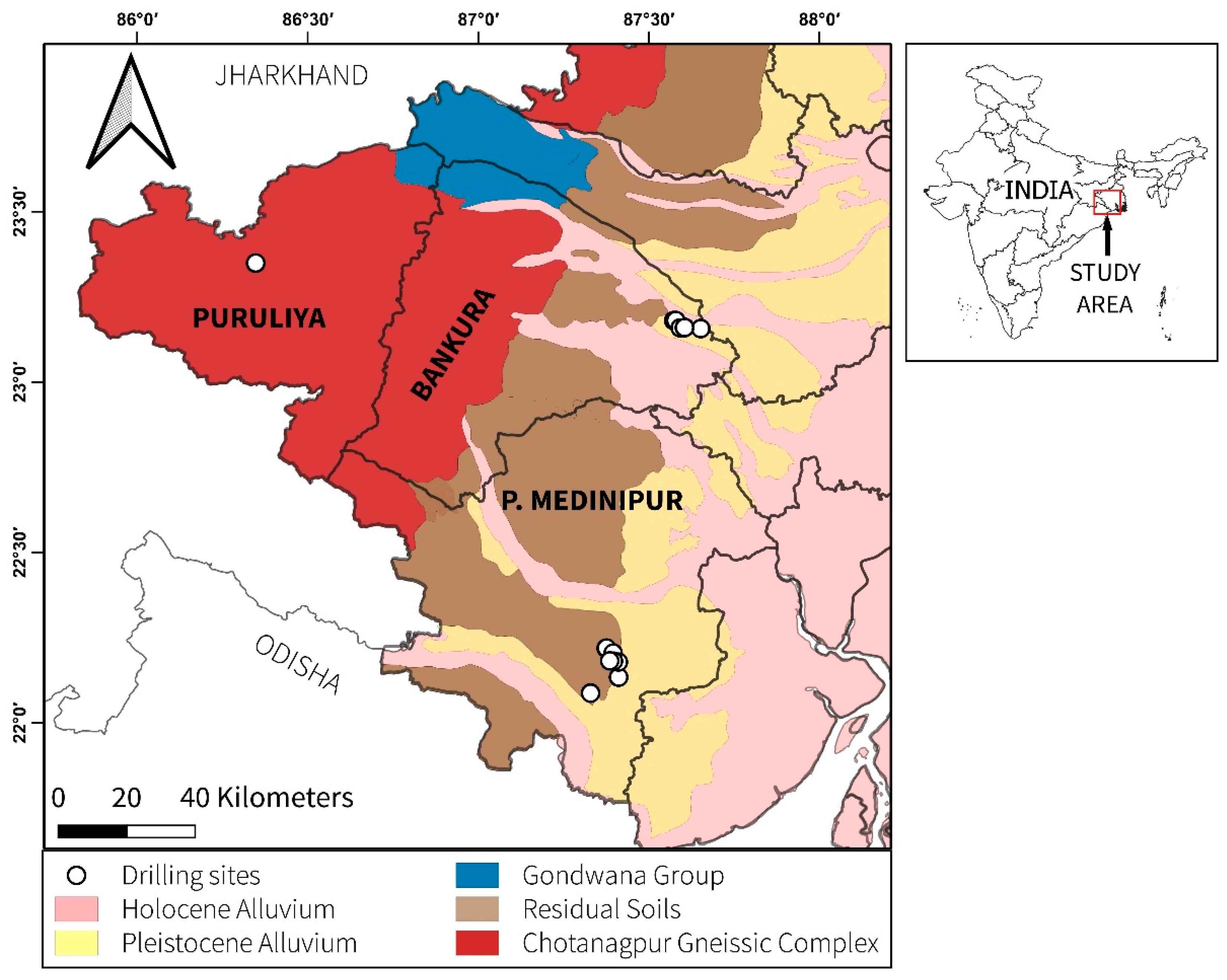
2.1. Study Area

The study area comprises the three districts of Bankura, Puruliya, and Paschim Medinipur (P. Medinipur) in West Bengal, India. The study area demonstrates three different geological terrains, i.e., CGC, Residual Soils, and Pleistocene Alluviums. The 3 districts were selected for the study as there have been reported incidences of fluorosis and elevated groundwater F occurrences in the area [15,17,19]. Another reasoning for the selection of drilling sites in the area is the occurrences of F-bearing minerals in the subsurface lithology [21,22], which may be susceptible to leaching F into the groundwater.
Bankura district comprises older to newer alluviums, with laterite blocks as nodules in some places [48]. The pediment–peneplain complex with the relatively broad and flat surface of bedrocks of denudational origin forms the landform of the region. Hills and mounds of the Puruliya district are generally formed from granitic rocks, which show planar banding of alternate layers of feldspar phenocrysts. The finer-grained assemblage of quartz; feldspar is also found in the area [49]. P. Medinipur district faces a water scarcity situation for irrigation and domestic water purposes [50]. Hard-rock upland, laterite-covered fringe areas, and flat alluvial plains are the main geomorphological features of the P. Medinipur district [51]. North-west and south-west parts of the district possess irregular terrain composed of laterite. However, the eastern part of the district is mostly gentle in gradient. The main source of recharge in the area is the percolation of rain and river water.
Sand and silts form the sub-surface of Pleistocene Alluvium terrain drilling sites; intrusive granites and quartzites in CGC terrain and quartz, phyllites, granites pebbles, and gravels, sand with silts, clay impregnated with caliche nodules, and Al, Fe hydroxides below the Residual Soils. The aquifer in the Pleistocene Alluvium terrain is composed of unconsolidated quaternary sand silt and clay with faulted structure and high permeability; Paleoproterozoic to upper Pleistocene crystalline aquifer with fissures, faults, and foliation and upper Pleistocene to Holocene sand silt and clay with very high permeability underneath the Residual Soils, and Pleistocene to recent semiconfined crystalline aquifer formed of faults, bedding planes and foliation underneath the CGC (Figure 1).

2.2. Groundwater Sampling and Analysis

Twenty-nine groundwater samples were collected around the borehole sites from the three geological terrains encompassed by the study area from hand-pumped tube wells following the procedures of Mukherjee and Fryar [52] in June 2022. The depth of the wells varies between 12 to 80 m and represents shallow aquifers. Groundwater samples were collected from the tube wells after purging them for several minutes until a constant temperature and electrical conductivity was recorded and then filtered through a 0.45 μm membrane filter. Essential physicochemical parameters such as pH, EC (electrical conductivity), TDS (Total dissolved solids), salinity, and temperature were measured using a portable handheld meter (Thermo Scientific, Eutech PCSTestr 35, Waltham, MA, USA). The major cation samples were preserved by adding 6N HNO3 to reduce the pH to ~2, while the anion samples were added CHCl3. Samples collected for estimation of alkalinity were collected without any headspace or preservatives.
The collected groundwater samples were analyzed on the subsequent days of sampling at IIT Kharagpur. The cation samples were analyzed in an ion chromatograph (Thermofisher, Dionex ICS-2100, Waltham, MA, USA), while the anion samples were analyzed in an ion chromatograph (Metrohm, 883 Basic IC Plus, Herisau, Switzerland). Total alkalinity (as CaCO3), HCO3 and CO32− were calculated by titration with 0.1 N H2SO4 by the inflection point method using the US Geological Survey alkalinity calculator.
Saturation index (SI) indicates, thermodynamically, whether water will tend to dissolve or precipitate a particular mineral and is expressed as the ratio between the chemical activities of the dissolved ions of the mineral (Ion Activity Product, IAP) and their solubility product (Ksp).
S I = l o g ( I A P K s p )
If SI = 0, it indicates that the mineral and the solution are at equilibrium; SI < 0 reflects that the solution is under-saturated with respect to the mineral; SI > 0 indicates that the solution is supersaturated with respect to the mineral, which would lead to the precipitation of the mineral [53].
Saturation indices (SI) with PHREEQC [54] (USGS, Version 3.4.0.12927, USA) using the WATEQ4F database were calculated to understand the thermodynamics of the stable mineral phases with the groundwater. This calculation distributes the total concentration of elements in a solution using an aqueous model to find the activities of the aqueous species. In the absence of data of redox couples and electron activity (pe), a default pe = 4.0 was used to calculate the SI of the solution.

2.3. Groundwater F Prediction Model

Groundwater F data (n = 205) from the Central Groundwater Board (CGWB) [55] was used to develop the groundwater F prediction model and the population map exposed to elevated groundwater F in the study area. CGWB collects groundwater samples during the pre-monsoon season every year from their hydrograph monitoring stations and analyzes them for groundwater quality. For analyzing F, ion-selective electrodes were utilized.
For the prediction of groundwater F in the study area, 15 predictor variables were used, i.e., area irrigated with groundwater, precipitation, temperature, aridity, potential evapotranspiration (PET), topographic slope, topographic wetness index, depth to the water table, fluvisols, subsoil pH, and cation exchange capacity, topsoil pH, and cation exchange capacity, geotectonic, and hydraulic conductivity. The supporting information Text S1 includes the details for the selection of these variables as predictors and details on the type and spatial resolution of the variables are provided in Table S1. Here, we apply random forest, a machine learning algorithm, to predict groundwater F occurrence using 15 predictor variables and groundwater F data from the study area.
Random Forest (RF) is a supervised learning approach that grows multiple decision trees to form a ‘forest’ and provide outputs. Individual trees in the RF model are supplied with a random subset of the data, hence called ‘random’ [56]. A randomly chosen portion of the training data is used to supply each decision tree employing the bagging method, and a subset of randomly selected predictor variables are provided at each split-node (split selection) to add randomization [57]. The introduction of randomness leads to the distinct formation of each tree in the model. Thus, all the information embedded in the data can be incorporated into the model, subsequently developing a robust model and therefore, RF is tolerant to issues like the presence of predictor variables multicollinearity, noise, outliers, and overfitting [58,59]. We have tested the continuous variables for the existence of any collinearity (Figure S1) based on Pearson correlation among them. If any two variables showed correlation > 0.80 (both positive and negative), the variables can be considered collinear. In this case, only topsoil and subsoil cation exchange capacity showed a correlation >0.80 [28]. However, as RF models are tolerant to multicollinearity, we retained these two variables in the model. RF is well-known for showing highly accurate results for classification and regression problems [60,61,62]. For classification predictions, each decision tree produces binary classes as an output based on probabilities and a cutoff value. The highest-voted class from the ensemble of all the trees in the forest serves as the final output of the model [56].
Each tree (Ti) in the RF model is fed with the random data subset consisting of p predictor variables out of total P predictors. Predictors with the best split and the split points are then fixed. The trees are then formed by splitting the data into fixed splitting points. Repeating this with new bagged data, the ensemble of the desired number of trees (N) is formed [60], and the most voted tree class is considered the final model output.
R ( P ) = 1 N n = 1 N T i ( p )
where R is the target variable in binary form. In this study prior to the development of the RF model, the groundwater F concentrations exceeding 1.0 mg/L were binary-classified into 1 and those ≤1.0 mg/L, were classified as 0. The entire dataset used to develop the RF model (n = 205) comprised mostly ≤1.0 mg/L F concentrations (87.4%) and very less (12.6%) concentrations exceeded 1.0 mg/L, indicating an imbalance in the dataset. Thus, we have applied the downsampling with the replacement method embedded in the RF model to supply trees with an equal number of 0 (i.e., ≤1.0 mg/L F) and 1 (>1.0 mg/L F) data [27]. This downsampling with the replacement method enabled the model to handle an imbalance in the data without any information loss. The entire dataset was split in an 80:20 ratio to train and test datasets. To tune the RF model for the most accurate outputs, the number of trees and the number of randomly selected predictors at each split node can be altered. The performance of the RF model was assessed using the parameters like accuracy, sensitivity, specificity, and area under the curve (AUC) value from the receiver operating characteristic (ROC) curve. The cutoff value for the classification was fixed using the intersect (or trade-off) of the sensitivity and specificity [27,63]. The out-of-bag (OOB) error rate is also an internal performance analysis parameter, and this was calculated over one-third of the training dataset that was held out during the formation of each tree in the model [64]. The OOB error rate helps to understand the balance between train and test set splits [16]. An important property of the RF model is the determination of the relative importance of the predictor variables, which was determined as the mean decrease in the accuracy of the model. In case, the mean decrease in the accuracy value of the model is very high due to the removal of an individual variable, the variable is considered to have higher relative importance. The RF modeling was executed in the R software using the ‘randomForest’ package [65].

2.4. Sediment Sampling and Analysis

To understand the influences of unsaturated zone F inventory on the groundwater F concentrations, three types of land use patterns were identified, i.e., agricultural land, grasslands land, and forest land from three different geological terrains, viz., CGC, Residual Soils, and Pleistocene Alluviums, where dry drilling at 25 locations was done up to a depth of ~10 m. Dry sediment samples were recovered with a hand auger with inter-changeable nickel-coated iron rods in July 2016. The diameter of the auger was 20 cm. This auger was rotated manually to an average depth of 3 m and pulled out on the surface with the help of a 15 m tripod set. The very hard nature of the subsurface in some locations restricted us from using a hollow iron stem catcher inserted in the subsurface with a 15 kg hammer from the tripod setup.
Bulk sediment of ~200 g sample size was collected at ~0.15 m depth intervals for the initial top 1.5 m and each 0.3 m depth intervals beyond 1.5 m. Samples were then placed in air-tight plastic cups, sealed using para-films or plastic tapes, and then further sealed in air-tight polyethylene bags to minimize drying of the samples.
A total of 324 unsaturated zone sediment samples were collected, which were analyzed for their water-soluble concentrations of anions (Cl, F, SO42−, NO3, and PO43−). 25 g of sediment was taken in centrifuge tubes where 40 mL of ultrapure water was added. The mixture was shaken and then centrifuged at 7000 rpm for 4 h, and 45 min, respectively, to separate water from sediment. The supernatant was filtered (using a 0.22 μm pore-sized membrane filter) before analysis by an ion chromatograph (Metrohm, 883 Basic IC, Herisau, Switzerland). To determine the gravimetric water content the residual sediments in the centrifuge tubes were then oven-dried at 105 °C for 48 h. For the water-extractable ion concentration to be expressed on a mass basis as milligrams of ion per kilogram of dry sediment the supernatant concentration was multiplied by extraction ratio (g water/g sediment) and divided by water density. The mass concentrations (mg/kg) were divided by the gravimetric water content and then multiplied by the density of water (997 kg/m3) to get the ion concentrations in milligrams of ion per liter (mg/L). To account for the water loss during sample collection and processing, which may overestimate ionic concentrations when expressed as mg/L, ionic concentrations on a mass basis (mg ion/kg dry sediment) are considered more reliable. For determination of elemental composition and mineral phase identification by energy dispersive X-ray fluorescence (XRF) method (Malvern Panalytical, Epsilon 3, Malvern, UK) and X-ray diffraction (XRD) method (Malvern Panalytical, ‘X’Pert Powder, Malvern, UK), respectively, the sediment samples (10 g) were oven-dried at 60 °C for 8 h, hand-grounded in a mortar and pestle and subsequently sieved through an ASTM 200 mesh (75 μm). The mineral phases were quantified by Cu Ka radiation and a positive-sensitive detector of X-ray diffraction with 20 mA current and 30 kV accelerating voltage. The generated XRD peaks were processed in the ‘X’Pert HighScore software (Malvern Panalytical, Malvern, UK) to search-match with the ICSD reference database for the identification of mineral phases.

3. Results

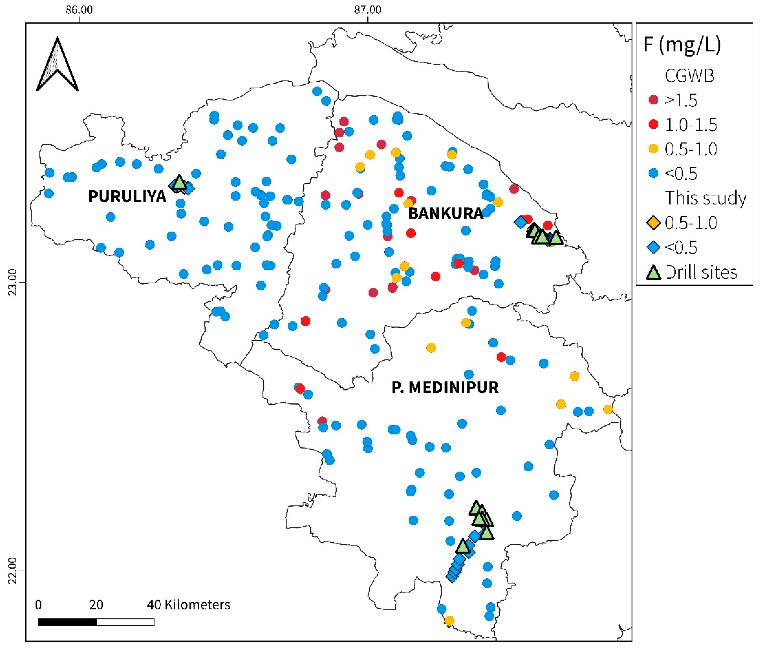
3.1. Groundwater Chemistry and F Distribution

The maximum (mean) concentration of groundwater F in the vicinity (within 5 km) of the drilling sites in the Residual Soils, CGC, and Pleistocene Alluvium terrains are 0.4(0.2), 0.6(0.4), and 0.6(0.3) mg/L, respectively. The spatial distribution of groundwater F in the study area is shown in Figure 2, and the statistical summary of measured groundwater chemistry is shown in Table 1. Groundwater has a neutral pH in Pleistocene Alluvium terrain (mean pH 6.9), Residual Soils terrain (mean pH 6.5), and CGC terrain (mean pH 6.7). Groundwater F in the study area, however, does not exceed the WHO permissible limit (1.5 mg/L). The mean groundwater F in the three borehole locations is also lower than the optimal range (0.7 mg/L) [66] Groundwater of the study area is fresh (TDS < 1000 mg/L) and has naturally evolved without significant hydrogeochemical processes (Ca-Na-HCO3 hydrogeochemical facies). It has a moderate hardness in Pleistocene Alluvium and Residual Soils, while in CGC it is hard, although it is temporary (carbonate hardness). The average concentrations of the major cations are in the order of Ca > Na > Mg > K, and the major anions are in the order of HCO3 > Cl > SO4 > NO3 > F > CO3.

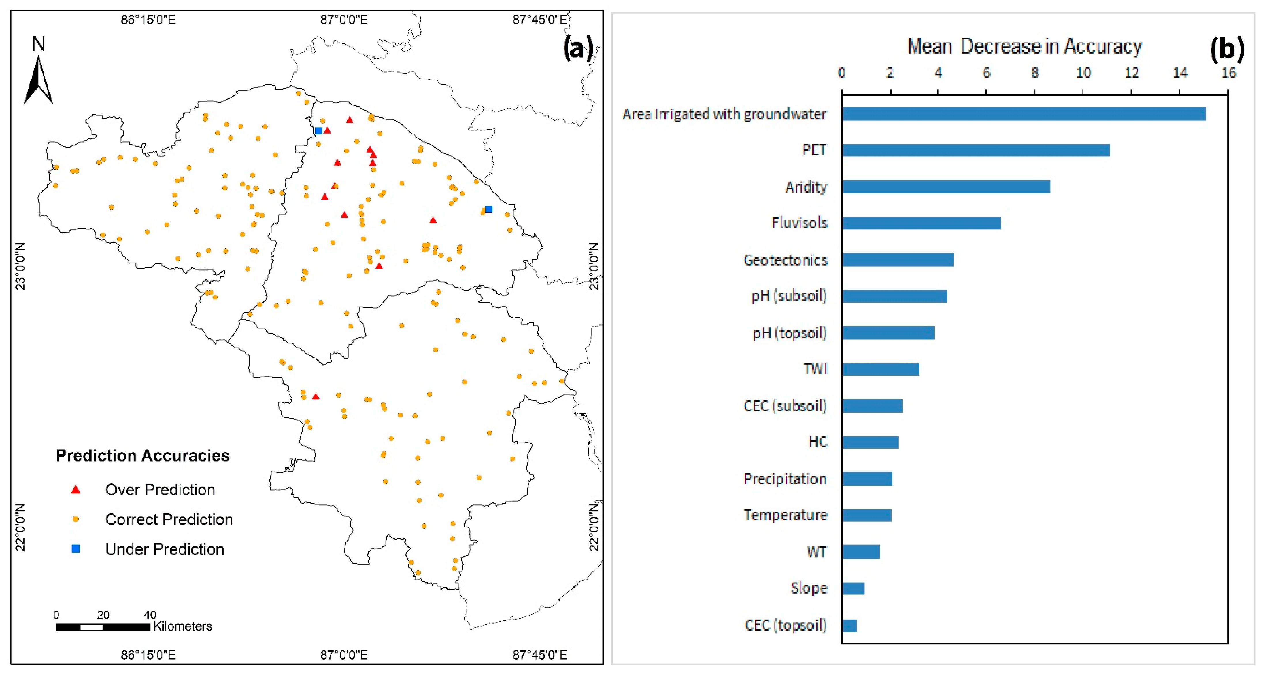
3.2. Model Prediction of the F Distribution

The RF model developed here incorporated 1200 trees and the number of random predictor variables provided at each split-node was four (the closest integer number to the square root of the number of predictor variables). The RF model achieved an accuracy of 90% and AUC of 0.95 with a cut-off value of 0.55 for the test dataset fixed from the intersection of the sensitivity and specificity (Table S2 and Figure S2). Furthermore, the model showed accuracy and AUC values of 93% and 0.99 using a cutoff of 0.58 for the entire dataset, respectively (Table S2 and Figure S3). The accuracy of the training dataset was 91% (Table S1). The model showed an OOB error rate of 35.15%, which indicate a good split between the train and test set. The model also achieved balanced sensitivity and specificity values for all the datasets, which suggested that the model successfully handled the imbalance in the data (Table S2). These results depict the significant prediction ability of the model. Therefore, the RF model was used to produce the probabilistic occurrence of groundwater F above 1.0 mg/L for the three districts in the western part of WB, i.e., Bankura, Puruliya, and P. Medinipur, which roughly conform to the three geological terrains, viz., Pleistocene Alluvium, CGC, and Residual Soils, respectively, at 1 km resolution—the same resolution of the majority of the predictor variables.
The random forest model predicted the probability of occurrence of F (>1.0 mg/L) for the study area and generated the F probability map (Figure 3a). The model predicts discrete pockets of the high probability (>0.55) of groundwater F (>1.0 mg/L) in the entire study area with higher occurrences in Bankura. The predicted occurrence from the random forest model is consistent with the measured F levels in the groundwater. The field surveyed groundwater F measurements (n = 29) were used to validate the RF model. The validation yielded a high accuracy of 96% with a sensitivity of 0.96 (Table S2). The sensitivity indicates that the model has good accuracy in classifying elevated (>1.0 mg/L) groundwater F. Figure 3b shows the population exposed to elevated groundwater F, generated using the predicted probabilities of the random forest model. The population exposure map indicates that in Bankura, 0.2 million (4% of the total population), 0.1 million (1.7%) in P. Medinipur, and 0.1 million (2.6%) in Puruliya may be exposed to elevated groundwater F. The model mostly makes correct predictions for Puruliya and P. Medinipur, except for a few over and under predictions in Bankura (Figure 4a). RF model predicts 281 km2 area (4% of the land area) in Bankura to have a high (>0.55) probability of elevated (>1.0 mg/L) groundwater F, while in Puruliya and P. Medinipur it is 167 km2 (2.6 %) and 175 km2 (1.8%), respectively.
Among the 15 variables used for modeling, “area irrigated with groundwater”, “aridity”, and “potential evapotranspiration (PET)” have the highest mean decrease in accuracy, while “temperature”, “depth to the water table (WT)”, and “topsoil cation exchange capacity (CEC)” are among with least mean decrease in accuracy (Figure 4b). Other variables with a moderate mean decrease in accuracy are “fluvisols”, “geotectonic”, “subsoil pH” and “topsoil pH” (Figure 4b).

3.3. Model Limitations

The model only represents the 2D spatial distribution of F in groundwater on a regional scale and holds with the measured F concentrations in groundwater. The predictions of elevated groundwater F developed here do not represent depth-wise or well-to-well F concentrations. However, the occurrence of F is also depth-sensitive; therefore, including other depth-regulated variables is likely to provide more accurate predictions. The 1 km resolution used here to develop the predictions was selected due to better model outputs. The majority of the predictors have a resolution of 1 km and may have caused such results. Furthermore, the estimation of the population exposed to elevated groundwater F does not account for factors such as the use of alternative sources, consumption rates, duration of exposure, treatment of water, or F awareness, which are significant for a more accurate F exposure assessment. The incorporation of such factors can provide further precise estimations.

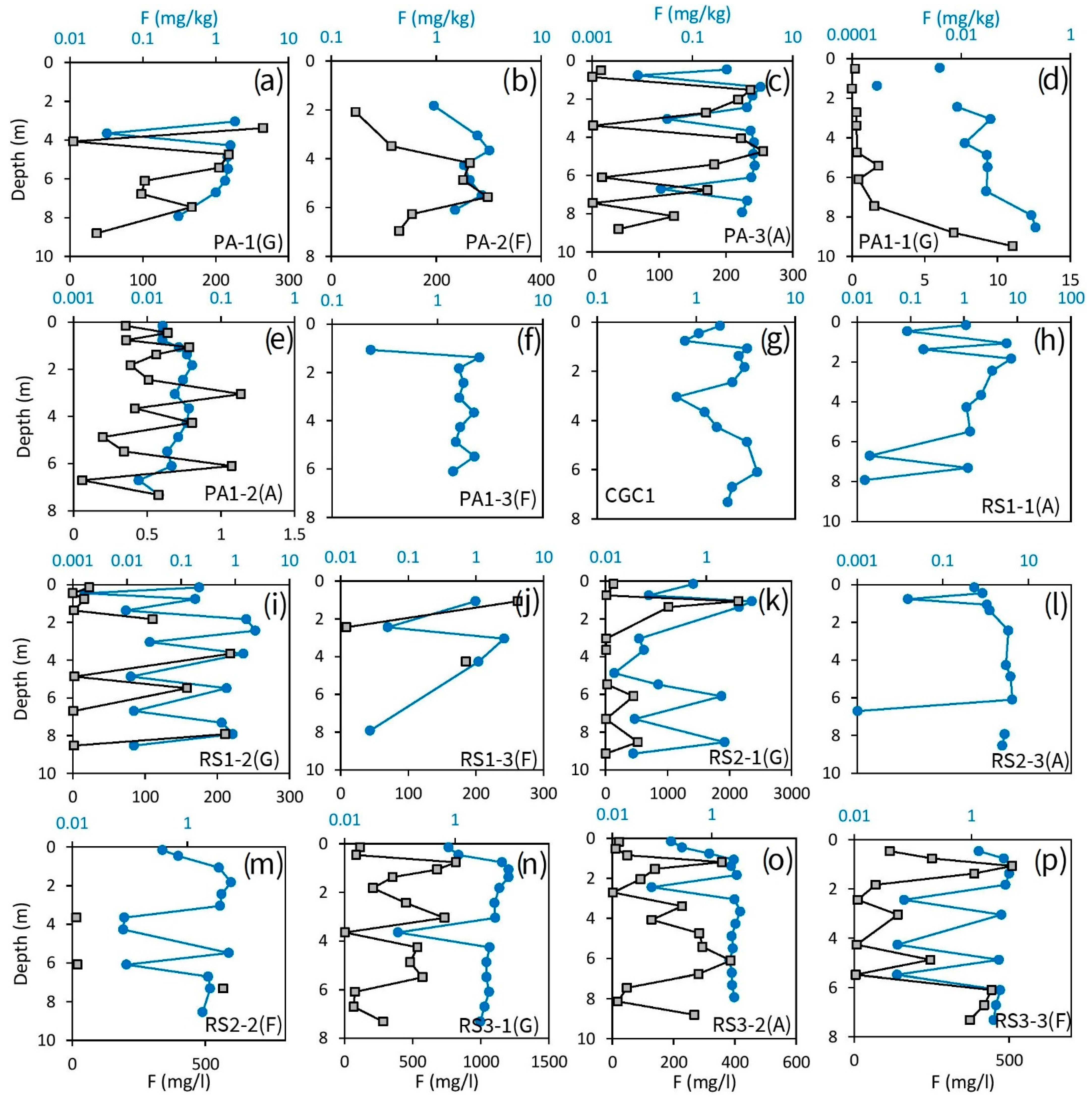
3.4. Unsaturated Zone F profile

The unsaturated zone F concentration we present here is derived from the weathered (~10 m) zones above the subsurface regolith. The drilled sites’ sediment F profiles with depth are shown in Figure 5a–p. CGC has the highest unsaturated zone F concentration (mean 2.2 mg/kg), followed by Residual Soils (mean 1.6 mg/kg) and Pleistocene Alluviums (mean 0.7 mg/kg). Forest-covered land in Pleistocene Alluviums has significantly higher normalized unsaturated zone F inventory (120 kg/ha/m) compared to agricultural (56 kg/ha/m) and grasslands (58 kg/ha/m) land. Unsaturated zone F profile in CGC (Figure 5g) does not show any significant trend, showing peak bulges at 1 and 6 m depth. The profiles from Pleistocene Alluviums (Figure 5a–f) show higher F concentrations within 1, and 6 m depth, whereas profiles from Residual Soils (Figure 5h–p) show a significant peak at ~1 m depth, below which it decreases gently with depth.

4. Discussion

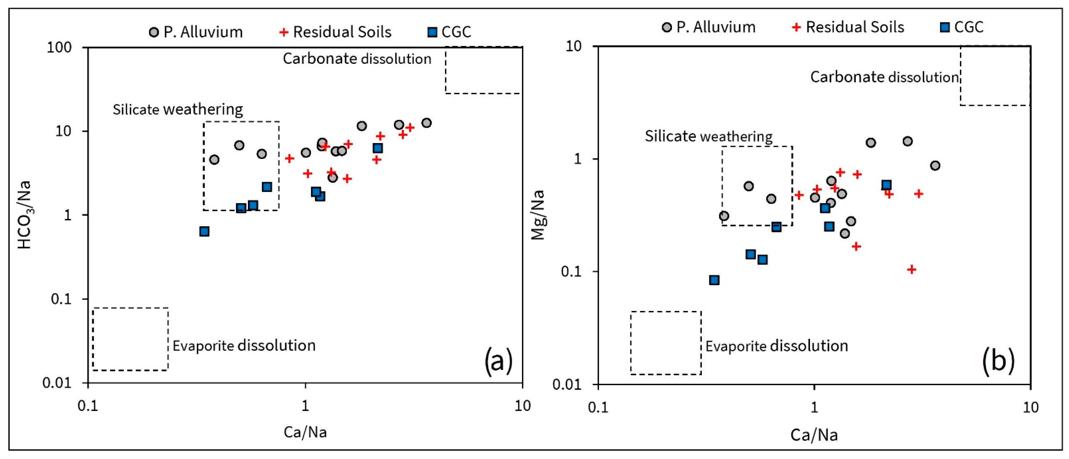
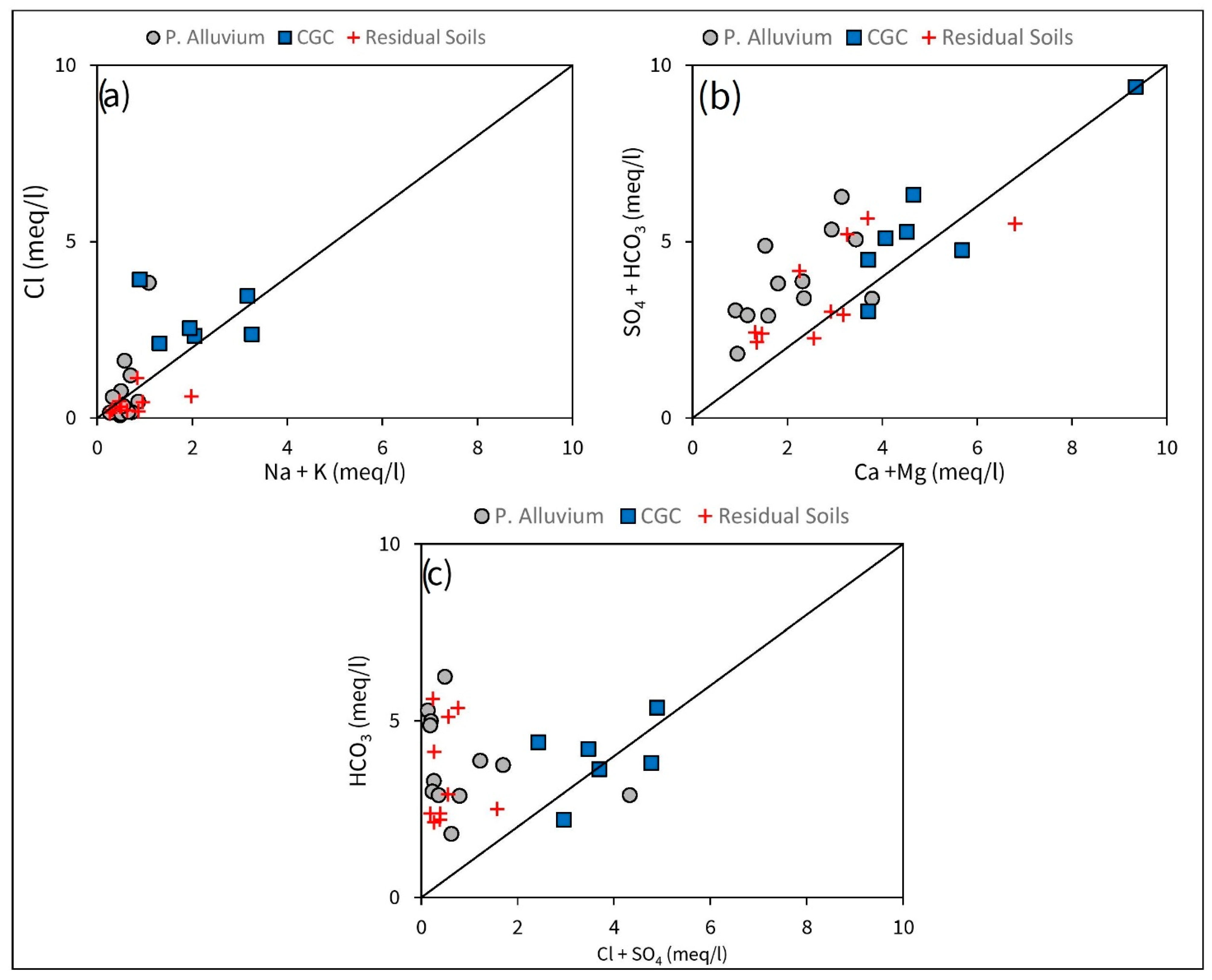
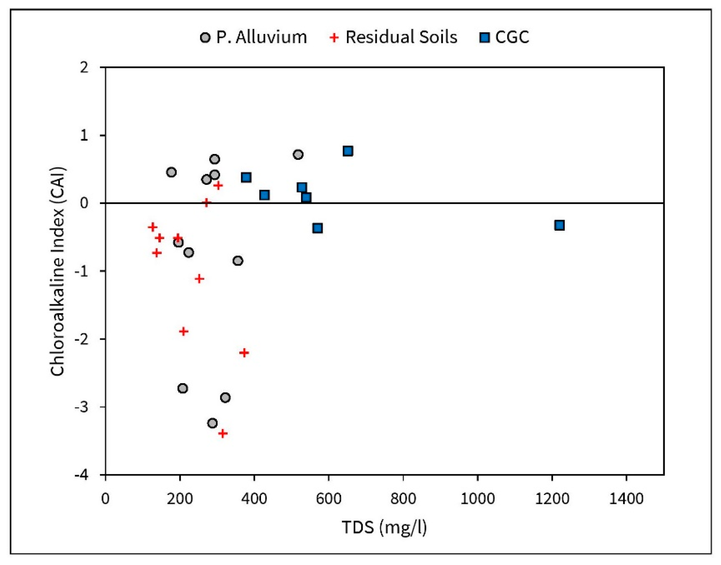
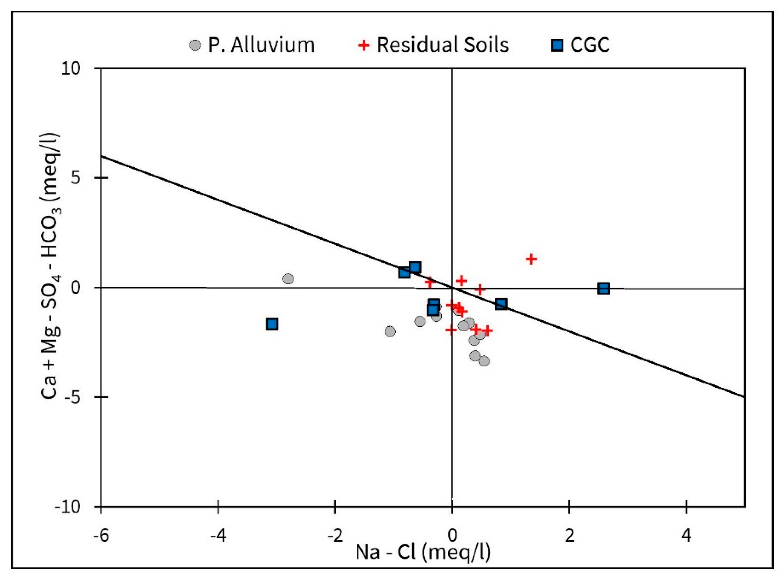
4.1. Hydrogeochemical Controls of F Mobilization

Groundwater F concentration is highest (maximum 0.6 mg/L) in Puruliya as per the groundwater samples collected, underlain by the CGC, followed by groundwater in Bankura (maximum 0.6), underlain by Pleistocene Alluviums, and groundwater in P. Medinipur (maximum 0.4), underlain by Residual Soils [67]. The occurrence of F in the groundwater of the study area has been attributed to the dissolution of F-bearing minerals found in the underlying rocks of the region [21,22]. The evolution of groundwater chemistry can be explained by tracing the origin of solutes, their dominance, and hydrogeochemical processes. Molar ratio bivariate plots such as Na-normalized Ca, Mg, and HCO3 can be used to ascertain whether solutes have been derived from the weathering of silicate rocks or the dissolution of carbonates and/or evaporites [68,69,70]. Here, silicate weathering, along with carbonate and evaporite dissolution, is found to control the evolution of the hydrochemistry of the study area, as evident from the bivariate plots (Figure 6a,b). (Na + K)/Cl milliequivalent ratio represents cation sources; a positive value indicates silicate weathering source, while a negative value indicates evaporite dissolution [71,72]. Figure 7a shows that most of the groundwater falls along the 1:1 line suggesting both silicate weathering and evaporite dissolution. In the (SO4 + HCO3) vs. (Ca + Mg) plot (Figure 7b), groundwater falls along the 1:1 line and some above it, which indicates the sources of Ca, and Mg to be dominantly silicate weathering [71,73]. The HCO3 vs. (Cl + SO4) plot (Figure 7c) shows that groundwater from Residual Soils terrain and Pleistocene Alluvium have dominance of carbonate dissolution over evaporite dissolution as the samples plot above the 1:1 line. In contrast, samples from CGC plots along the 1:1 line suggest both evaporite and carbonate dissolution [71]
(Na+, K+, Ca2+, Mg2+) silicates + H2CO3 → H4SiO4 + HCO3 + Na+ + K+ + Ca2+ + Mg2+ + Clay
Na and K ions may be removed from the solution by reverse cation exchange process, while Ca may be removed from the solution by cation exchange process (Equation (4)) with clay minerals as indicated by Chloroalkaline Index (CAI) vs. TDS graph (Figure 8). The CAI is calculated using the formula: CAI = [Cl − (Na+ + K+)]/Cl. A positive CAI indicates a reverse cation exchange process (Equation (4) would proceed toward the left), while a negative CAI indicates a forward cation exchange process (Equation (4) would proceed towards the right) [71]. A bivariate plot of (Ca2+ + Mg2+ − HCO3 − SO42−) vs. (Na+− Cl) (Figure 9) can also be utilized to understand ion exchange processes [71,74]. An excess of Na over Cl, deficiency of Ca + Mg over HCO3 + SO4, and a −1 slope indicate the cation exchange process and vice versa [71,73,75]. However, the plot (Figure 9) shows variable Ca, Mg, and Na ionic concentrations; moreover, groundwater of the study area has dominant Ca-Na-HCO3 hydrogeochemical facies suggesting that both cation and reverse cation exchange processes contribute to the hydrochemistry.
2Na+ + Caclay ↔ Ca2+ + 2Naclay
CO32− and HCO3 ions and the pH of groundwater control the dissolution of fluorite and F-rich minerals, as shown by Equations (5) and (6). Higher concentrations of CO32− and HCO3 ions favor the mobilization of F and precipitation of CaCO3.
CaF2 + CO32 → CaCO3 + 2F
CaF2 + HCO3 → CaCO3 + 2F + CO2 + H2O
Fluorite (CaF2) and calcite (CaCO3) are under-saturated to an equilibrium state in the groundwater system of all three geological terrains. The equilibrium condition of calcite and fluorite in the solution can be expressed by Equation (7), and the coupled solubility of calcite and fluorite is given by Equation (8). These equations suggest that the increase in the HCO3 coupled with the precipitation of CaCO3 would result in the increase of F in the solution.
CaCO3 + H+ + 2F → CaF2 + HCO3-
Kcalcite-fluorite(Eq) = [HCO3]/{[H+][F]2}
Equation (7) represents an essential process that releases F into groundwater, evident from the hydrochemistry. In all three geological terrains, where groundwater is mainly of HCO3 dominance, it suggests that Equation (7) would proceed towards the left. The presence of caliche nodules in the subsurface and under-saturation of calcite further indicates the development of this process. Saturation indices show whether a particular mineral phase would precipitate (oversaturated) from a solution or dissolve (undersaturated) from a stable phase into the solution [53]. Figure 10, which shows the SIfluorite vs. F concentration in groundwater, suggests that fluorite is undersaturated, and thermodynamically, it is possible that with an increase in residence time, groundwater F concentration may increase in CGC, and Residual Soils terrains owing to their elevated unsaturated zone F inventory until fluorite equilibrium is reached. The groundwater is also found to be undersaturated with halite (NaCl), anhydrite (CaSO4), and gypsum (CaSO4.2H2O), and the dissolution of these minerals could be the possible reason for high Cl and SO4 in the groundwater.

4.2. Significance of Predictor Variables

The RF model shows that the anthropogenic predictor variable “area irrigated with groundwater” has the highest importance in groundwater F prediction in the study area. Groundwater aquifers may be susceptible to vertical leaching by irrigation return flows and their interaction with the pore water, which may be an important driver of F migration [76]. Lowering the water table due to the extensive abstraction of groundwater for irrigation may also exacerbate F mobilization [76]. Subsequently, climate variables “PET” and “Aridity” have a relatively higher importance in predicting elevated groundwater F. Drier climate with increased evapotranspiration, corroborated by decreased precipitation and high temperature has been linked with groundwater F enrichment [3,23]. For the study area, the predicted probability of elevated (>1.0 mg/L) groundwater F is found to be more in the areas with lower precipitation and comparatively higher temperature and PET (Figure S4), like the Bankura district. Similar studies [16,77,78] also show a higher probability of elevated groundwater F occurrences in arid to semi-arid climates. Further, soil variables such as “fluvisols”, “subsoil pH”, and “topsoil pH” also have high importance. It is observed that areas with a lower % of fluvisols and soil pH (topsoil and subsoil) between 6.0–6.5 correspond with higher probabilities of elevated F predictions (Figure S4). The presence of fine-grained soils with higher clay and oxyhydroxide content, such as in fluvisols, may retain higher F than sandy soils [79]. Additionally, pH between 6.0–6.5 is suitable for F mobility in fine-grained soils [80,81]. “CEC” (topsoil) has the least importance among the predictor variables. Finally, the “geotectonics” of the region has been found to have strong control over the groundwater F prediction. CGC a part of the Craton shield (Figure S4) is abundant with F-bearing minerals [21,22], the weathering and dissolution of which may lead to groundwater F enrichment [23,82]. CGC, mainly composed of granitic-gneissic rocks, has also the highest normalized unsaturated zone F inventory (Table 2). Addison et al. [83] show >60% statistical likelihood of elevated groundwater F occurrence in rocks of alkaline igneous composition. Similarly, Ling et al. [77] also indicate lithology as an important predictor for groundwater F.
An analysis of the importance of predictor variables shows that the highest probability of elevated groundwater F can be expected in areas with geological formations abundant with F-bearing rocks in arid to semi-arid regions. However, increased groundwater abstraction for irrigation may aggravate groundwater F enrichment.

4.3. Fate of F and Impact of Unsaturated Zone Matrix

A comparison of F concentrations in the unsaturated zone and groundwater reveals that although Pleistocene Alluviums have the lowest sediment F inventories among the three geological terrains, it has relatively higher groundwater F concentrations. In contrast, Residual Soils, which have a higher sediment F inventory compared to Pleistocene Alluviums, have low groundwater F (Table 2). XRD analysis suggests the presence of micas, feldspars, pyroxenes, F-rich minerals (fluorite, sellaite, elpasolite, Laurelite), and minor clay and olivine in the sediments of Pleistocene Alluviums; quartz, feldspars, and F-rich minerals in CGC sites; and quartz, pyroxenes, F-rich minerals, calcite, apatite, garnets, clay minerals, and Fe, Al hydroxides in the sediments of Residual Soils terrain. The XRD and XRF analysis results are shown in Figure 11 and Table S3, respectively.
The lithology of the area plays a dominant role in the F distribution in the sediments. Sub-surface in Puruliya formed from the weathering of intrusive granites, granite gneiss, migmatites, and mica schists, which generally have a higher concentration of F in them. The major minerals found in the unsaturated zone of the study area are quartz, muscovite, feldspars, pyroxenes, calcite, clay, and F-rich minerals, as evident from XRD and XRF analysis. The subsurface beneath Residual Soils terrain is underlain by granites, phyllites, sand, silt, and clay impregnated with caliche nodules. In contrast, the subsurface of Bankura drilling sites is mainly composed of sand and silts of Older Alluvium. Calcrete is expected in the weathered zones of granitic/gneissic rocks. The mobility of unsaturated zone F is strongly dependent on the sorption capacity of the sediments, which changes with pH, sorbent types, and soil salinity [85]. Caliche nodules precipitated from calcite-rich rocks can have F concentrations ranging from 510 to 9000 ppm [23]. The formation of CaF2 and Ca5F(PO4)3 is the primary process of F retention in calcareous soils [81,86]. F can be removed from the solution during calcite precipitation, where F gets adsorbed on the surface of calcite [87], along with the precipitation of fluorite at step edges and kinks [88]. Clay minerals offer surface sites for F adsorption, having adsorption capacities ranging from 69.4–93.5 mg/kg [89]. Montmorillonite at pH~6 attracts negatively charged F ions by its positively charged surface [90]. Diop et al. [91] have demonstrated that synthetic clay minerals can be used for F removal under near-neutral to acidic conditions. Freshly precipitated Fe and Al hydroxides can adsorb much more F than clays and Fe, Al oxides [81]. Laboratory leaching experiments indicate that soil column containing primarily sand, in the absence of clays, can flush out up to 50% of F in it [92]. The observed conditions (Table 2) suggest that the unsaturated zone beneath Residual Soils, rich in clays, calcite precipitates, and Al, Fe hydroxides, retain significant dissolved F from solution, while the subsurface beneath Pleistocene Alluviums, mostly sand and silts, cannot prevent F from leaching out, thus facilitating high F groundwater.

4.4. Land-Use Patterns and F Distribution

Land-use patterns can significantly affect the infiltration of recharging rainwater and thus may control the leaching of soluble ions in the subsurface. The recharge rate was highest in agricultural land (132 mm/year), followed by grasslands (74 mm/year) and forest land (20 mm/year) in the study area (Table 2) [92]. Higher recharge rates, such as in agricultural and grassland land, can facilitate the leaching of soluble ions in the subsurface. In comparison, lower recharge rates under the forest covers could prevent ions such as F from leaching into the groundwater. This is quite evident in Pleistocene Alluviums, where agricultural and grasslands have been significantly flushed out of F compared to forest lands. The normalized unsaturated zone F inventory in the forest land of Pleistocene Alluviums is 121 kg/ha/m, while that of agricultural and grasslands lands is 56 and 58 kg/ha/m, respectively (Table 2). Sand and silty soil beneath the sub-surface may facilitate the mobilization of F with increased infiltration (Table 2). The absence of clay fractions and calcretes in the sub-surface of Pleistocene Alluviums allows the leaching of F by the infiltrating water. However, Scanlon et al. [41] have demonstrated that increased recharge through land-use changes has little effect on F mobilization in the subsurface of semi-arid regions. In contrast, the same regions show increased mobility of Cl with increasing recharge. F has also been found to be less sensitive to variation in infiltration rate in irrigated lands [93]. Beneath Residual Soils, the different land-use patterns do not show any marked variation in their normalized unsaturated zone F inventories (agricultural land = 218 kg/ha/m, forest land = 202 kg/ha/m, and grasslands = 228 kg/ha/m), although they show variations in their recharge rates (Table 2). Lesser leaching beneath Residual Soils could be attributed to the presence of clay minerals, Fe, Al hydroxides, and secondary precipitates of calcites. The low F content in the unsaturated zone at <1 m depth within the soil root zone in all the sites could be ascribed to the water and nutrient uptake process by the roots of plants where they absorb F from the soil, and also subsequently, under certain conditions, get desorbed by water and inert salt solutions [94]. Our model predictions suggest land-use patterns to have less significance in the prediction of F distribution in the study area.

4.5. Implications for Groundwater F Pollution

Evidence suggests that a moderate level of F intake can prevent dental caries and also promote the development of strong bones, under certain conditions [3,95,96]. An estimated about 0.4 million people in the study area within Bankura, Puruliya, and P. Medinipur in West Bengal could be exposed to groundwater F (>1.0 mg/L), where F intake is primarily through drinking water. Such exposures can lead to the development of dental as well as skeletal fluorosis, especially in children, particularly Bankura district with elevated groundwater F. Elevated groundwater F regions, where heavy abstraction of groundwater is used for irrigation, could also be at additional risk from bioaccumulation of F in the agricultural produce. High abstraction of groundwater may lead to pumping-induced increased groundwater recharge [33]. With enhanced recharge, water-soluble ions and contaminants from the land surface and unsaturated zone gets mobilized into the groundwater [45,97] Defluoridation measures using activated alumina [98], and lime [99] which can effectively remove F from drinking water supplies, can be used in elevated groundwater F areas; whereas, in regions with low groundwater F, fluoridation of water supply can ensure an optimal (0.7 mg/L) F level [66] in the drinking water. Activated alumina, alum, lime, and clays can remove F from drinking water with up to 90 % efficiency based on adsorption and precipitation processes, which is also quite evident in the subsurface of the study area. AI-based algorithms such as random forest, used in this study, can predict the occurrence of the groundwater F distribution with reasonable accuracy and also can be used to predict the occurrence of other groundwater pollutants. Models derived from studies like this can help identify areas exposed to groundwater pollutants and help drillers and authorities explore safe drinking water resources.

5. Conclusions

Unsaturated zone F is relatively immobile in the presence of clay-rich fractions, calcite, Fe, and Al hydroxides as they bind F to their structure very strongly and need suitable pH and thermodynamics in order to become flushed to deeper levels. In the absence of these F sinks within the unsaturated zone, an increase in recharge rates through a change in land-use patterns can significantly mobilize F, such as in the agricultural and grasslands of Pleistocene Alluviums. CGC has the highest unsaturated zone F content, followed by Residual Soils, and Pleistocene Alluviums. However, elevated unsaturated zone F does not necessarily conform to elevated groundwater F as in the case of Residual Soils terrain and Pleistocene Alluviums. The sub-surface retention capacity, the formation of secondary calcite precipitates, and the presence of clay minerals, Fe, and Al hydroxides significantly influence F mobility. We suspect groundwater interaction with the unsaturated zone during water table fluctuations to have significant control on unsaturated zone F mobilization. Rock weathering followed by a reverse ion exchange process along with the dissolution of fluorite and F-rich minerals are the primary processes for forming elevated groundwater F in the study area. Occurrences of groundwater pollutants such as F can be predicted with reasonably high accuracy using AI-based algorithms such as the random forest model, where prediction models can identify safe drinking water resources. Further, the processes resulting in the retention of F in the unsaturated zone of the study area are corroborated by the use of materials such as alum, lime, and clays in F removal techniques from drinking water supplies.

Supplementary Materials

The following supporting information can be downloaded at: https://www.mdpi.com/article/10.3390/w14203220/s1, Text S1. Details of Predictors used for groundwater fluoride model. Table S1. List of variables selected for possible influence on groundwater Fluoride, their sources and relation with Fluoride based on previous literature. Table S2. Details of the Random forest model performance. Table S3: Details of groundwater F measurements (n = 205) from CGWB database and RF predicted area with elevated (>1.0 mg/L) groundwater F and estimated population exposed to elevated groundwater F for the 3 studied districts of WB. Table S4. Elemental oxide weight % of soil sediments derived from XRF analysis. Figure S1. Correlation among the continuous predictor variables used in the Random forest model. Figure S2. (a) Sensitivity vs. specificity of the Random forest model and selected cutoff for the test data, (b) Area under the curve (AUC) value determined from the Receiver operating characteristic (ROC) curve of the Random forest model for the test data. Figure S3. (a) Sensitivity vs. specificity of the Random forest model and selected cutoff for the overall data, (b) Area under the curve (AUC) value determined from the Receiver operating characteristic (ROC) curve of the Random forest model for the entire data. Figure S4. Maps of the predictor variables used in the Random forest model. [3,16,33,76,78,83,100,101,102,103,104,105,106,107,108,109,110,111,112,113,114,115,116].

Author Contributions

Conceptualization, A.M., P.M. and D.A.A.; methodology, P.M., S.S., D.A.A. software, D.A.A. and S.S.; validation, P.M., S.S. and D.A.A.; formal analysis, P.M., S.S., D.A.A.; investigation, P.M.; resources, A.M.; data curation, P.M. and D.A.A.; writing—original draft preparation, D.A.A., P.M. and S.S.; writing—review and editing, D.A.A., P.M. and A.M.; visualization, D.A.A. and S.S.; supervision, A.M.; project administration, A.M.; funding acquisition, A.M. All authors have read and agreed to the published version of the manuscript.

Funding

This work was supported by CSIR, Govt. of India, NET (File no. 09/081(1360)/2019-EMR-I) to David Anand Aind.

Data Availability Statement

All data used in this study are presented in the paper and the supplementary materials.

Acknowledgments

We acknowledge the Project “Understanding the extent and natural/Anthropogenic Control on Ground Water Recharge in Water Scarce Areas of Western Districts of West Bengal” funded by the Public Health Engineering Directorate, Government of West Bengal. The authors are thankful to the Department of Geology and Geophysics, School of Environmental Science and Engineering, IIT Kharagpur, for providing laboratory facilities. We would also like to thank several students who worked on laboratory analyses and also acknowledge the help from Gangadhar Puttunuru, Prabin Das, Binoy Debnath, and Amit Choudhury, for their help during the sampling and transportation of samples. The authors acknowledge the use of the PHREEQC program for the calculation of saturation indices (SI), and QGIS software for the preparation of maps.

Conflicts of Interest

The authors declare no conflict of interest.

References

  1. Subba Rao, N.; John Devadas, D. Fluoride Incidence in Groundwater in an Area of Peninsular India. Environ. Geol. 2003, 45, 243–251. [Google Scholar] [CrossRef]
  2. Arnesen, A.K.M. Availability of Fluoride to Plants Grown in Contaminated Soils. Plant Soil 1997, 191, 13–25. [Google Scholar] [CrossRef]
  3. Edmunds, W.M.; Smedley, P.L. Fluoride in Natural Waters. In Essentials of Medical Geology: Revised Edition; Springer: Dordrecht, The Netherlands, 2013; pp. 311–336. ISBN 9789400743755. [Google Scholar]
  4. Dabeka, R.W.; Mckenzie, A.D. Survey of Lead, Cadmium, Fluoride, Nickel, and Cobalt in Food Composites and Estimation of Dietary Intakes of These Elements by Canadians in 1986–1988. J. AOAC Int. 1995, 78, 897–909. [Google Scholar] [CrossRef] [PubMed]
  5. Ismail, A.I.; Hasson, H. Fluoride Supplements, Dental Caries and Fluorosis: A Systematic Review. J. Am. Dent. Assoc. 2008, 139, 1457–1468. [Google Scholar] [CrossRef]
  6. Oliveira, M.J.L.; Paiva, S.M.; Martins, L.H.P.M.; Ramos-Jorge, M.L.; Lima, Y.B.O.; Cury, J.A. Fluoride Intake by Children at Risk for the Development of Dental Fluorosis: Comparison of Regular Dentifrices and Flavoured Dentifrices for Children. Caries Res. 2007, 41, 460–466. [Google Scholar] [CrossRef]
  7. Symonds, R.B.; Rose, W.I.; Reed, M.H. Contribution of C1- and F-Bearing Gases to the Atmosphere by Volcanoes. Nature 1988, 334, 415–418. [Google Scholar] [CrossRef]
  8. Fejerskov, O.; Larsen, M.J.; Richards, A.; Baelum, V. Dental Tissue Effects of Fluoride. Adv. Dent. Res. 1994, 8, 15–31. [Google Scholar] [CrossRef]
  9. Izuora, K.; Twombly, J.G.; Whitford, G.M.; Demertzis, J.; Pacifici, R.; Whyte, M.P. Skeletal Fluorosis from Brewed Tea. J. Clin. Endocrinol. Metab. 2011, 96, 2318–2324. [Google Scholar] [CrossRef] [Green Version]
  10. Freni, S.C. Exposure to High Fluoride Concentrations in Drinking Water Is Associated with Decreased Birth Rates. J. Toxicol. Environ. Health 1994, 42, 109–121. [Google Scholar] [CrossRef]
  11. Xiong, X.Z.; Liu, J.L.; He, W.H.; Xia, T.; He, P.; Chen, X.M.; Yang, K.D.; Wang, A.G. Dose-Effect Relationship between Drinking Water Fluoride Levels and Damage to Liver and Kidney Functions in Children. Environ. Res. 2007, 103, 112–116. [Google Scholar] [CrossRef]
  12. Viswanathan, G.; Jaswanth, A.; Gopalakrishnan, S.; Siva ilango, S.; Aditya, G. Determining the Optimal Fluoride Concentration in Drinking Water for Fluoride Endemic Regions in South India. Sci. Total Environ. 2009, 407, 5298–5307. [Google Scholar] [CrossRef] [PubMed]
  13. Heller, K.E.; Eklund, S.A.; Burt, B.A. Dental Caries and Dental Fluorosis at Varying Water Fluoride Concentrations. J. Public Health Dent. 1997, 57, 136–143. [Google Scholar] [CrossRef] [PubMed]
  14. Shah, S.; Bandekar, K. IS 10500: 91 Drinking Water Compared to WHO Guidelines. Indian Waterworks Assoc. 1993, 30, 179–184. [Google Scholar]
  15. Asian Deveopment Bank. Arsenic and Fluoride in Drinking Water in West Bengal: Characteristics, Implications, and Mitigation; Asian Deveopment Bank: New Delhi, India, 2020. [Google Scholar]
  16. Podgorski, J.E.; Labhasetwar, P.; Saha, D.; Berg, M. Prediction Modeling and Mapping of Groundwater Fluoride Contamination throughout India. Environ. Sci. Technol. 2018, 52, 9889–9898. [Google Scholar] [CrossRef] [Green Version]
  17. Samal, A.C.; Bhattacharya, P.; Mallick, A.; Ali, M.M.; Pyne, J.; Santra, S.C. A Study to Investigate Fluoride Contamination and Fluoride Exposure Dose Assessment in Lateritic Zones of West Bengal, India. Environ. Sci. Pollut. Res. 2015, 22, 6220–6229. [Google Scholar] [CrossRef]
  18. Mondal, N.K.; Pal, K.C.; Kabi, S. Prevalence and Severity of Dental Fluorosis in Relation to Fluoride in Ground Water in the Villages of Birbhum District, West Bengal, India. Environmentalist 2012, 32, 70–84. [Google Scholar] [CrossRef]
  19. Das, K.; Mondal, N.K. Dental Fluorosis and Urinary Fluoride Concentration as a Reflection of Fluoride Exposure and Its Impact on IQ Level and BMI of Children of Laxmisagar, Simlapal Block of Bankura District, W.B., India. Environ. Monit. Assess. 2016, 188, 1–14. [Google Scholar] [CrossRef]
  20. Majumdar, K.K. Prevalence of Fluorosis and Pattern of Domestic Filters Use in Two Fluoride Endemic Blocks of West Bengal, India. J. Compr. Heal. 2015, 3, 17–30. [Google Scholar] [CrossRef]
  21. Bhattacharya, H.N.; Chakrabarti, S.; Chakrabarti, S.; Bhattacharya, H.N. Incidence of Fluoride in the Groundwater of Purulia District, West Bengal: A Geo-Environmental Appraisal. Curr. Sci. 2011, 101, 152–155. [Google Scholar]
  22. Chakrabarti, S.; Bhattacharya, H.N. Inferring the Hydro-Geochemistry of Fluoride Contamination in Bankura District, West Bengal: A Case Study. J. Geol. Soc. India 2013, 82, 379–391. [Google Scholar] [CrossRef]
  23. Jacks, G.; Bhattacharya, P.; Chaudhary, V.; Singh, K.P. Controls on the Genesis of Some High-Fluoride Groundwaters in India. Appl. Geochemistry 2005, 20, 221–228. [Google Scholar] [CrossRef]
  24. Handa, B.K. Geochemistry and Genesis of Fluoride-Containing Ground Waters in India. Ground Water 1975, 13, 275–281. [Google Scholar] [CrossRef]
  25. Borgnino, L.; Garcia, M.G.; Bia, G.; Stupar, Y.V.; Le Coustumer, P.; Depetris, P.J. Mechanisms of Fluoride Release in Sediments of Argentina’s Central Region. Sci. Total Environ. 2013, 443, 245–255. [Google Scholar] [CrossRef]
  26. Banerjee, A. Groundwater Fluoride Contamination: A Reappraisal. Geosci. Front. 2015, 6, 277–284. [Google Scholar] [CrossRef] [Green Version]
  27. Sarkar, S.; Mukherjee, A.; Gupta, S.D.; Bhanja, S.N.; Bhattacharya, A. Predicting Regional-Scale Elevated Groundwater Nitrate Contamination Risk Using Machine Learning on Natural and Human-Induced Factors. ACS ES&T Eng. 2022, 2, 689–702. [Google Scholar] [CrossRef]
  28. Chakraborty, M.; Sarkar, S.; Mukherjee, A.; Shamsudduha, M.; Ahmed, K.M.; Bhattacharya, A.; Mitra, A. Modeling Regional-Scale Groundwater Arsenic Hazard in the Transboundary Ganges River Delta, India and Bangladesh: Infusing Physically-Based Model with Machine Learning. Sci. Total Environ. 2020, 748, 141107. [Google Scholar] [CrossRef]
  29. Singha, S.; Pasupuleti, S.; Singha, S.S.; Singh, R.; Kumar, S. Prediction of Groundwater Quality Using Efficient Machine Learning Technique. Chemosphere 2021, 276, 130265. [Google Scholar] [CrossRef]
  30. Malakar, P.; Mukherjee, A.; Bhanja, S.N.; Sarkar, S.; Saha, D.; Ray, R.K. Deep Learning-Based Forecasting of Groundwater Level Trends in India: Implications for Crop Production and Drinking Water Supply. ACS ES&T Eng. 2021, 1, 965–977. [Google Scholar] [CrossRef]
  31. Malakar, P.; Mukherjee, A.; Bhanja, S.N.; Ray, R.K.; Sarkar, S.; Zahid, A. Machine-Learning-Based Regional-Scale Groundwater Level Prediction Using GRACE. Hydrogeol. J. 2021, 29, 1027–1042. [Google Scholar] [CrossRef]
  32. Bhanja, S.N.; Malakar, P.; Mukherjee, A.; Rodell, M.; Mitra, P.; Sarkar, S. Using Satellite-Based Vegetation Cover as Indicator of Groundwater Storage in Natural Vegetation Areas. Geophys. Res. Lett. 2019, 46, 8082–8092. [Google Scholar] [CrossRef]
  33. Bhanja, S.N.; Mukherjee, A.; Rangarajan, R.; Scanlon, B.R.; Malakar, P.; Verma, S. Long-Term Groundwater Recharge Rates across India by in Situ Measurements. Hydrol. Earth Syst. Sci. 2019, 23, 711–722. [Google Scholar] [CrossRef] [Green Version]
  34. Malakar, P.; Mukherjee, A.; Bhanja, S.N.; Ganguly, A.R.; Ray, R.K.; Zahid, A.; Sarkar, S.; Saha, D.; Chattopadhyay, S. Three Decades of Depth-Dependent Groundwater Response to Climate Variability and Human Regime in the Transboundary Indus-Ganges-Brahmaputra-Meghna Mega River Basin Aquifers. Adv. Water Resour. 2021, 149, 103856. [Google Scholar] [CrossRef]
  35. Tylenda, C.A. Toxicological Profile for Fluorides, Hydrogen Fluoride, and Fluorine; Agency for Toxic Substances and Disease Registry: Atlanta, GA, USA, 2003. [Google Scholar]
  36. Barrow, N.J.; Ellis, A.S. Testing a Mechanistic Model. III. The Effects of PH on Fluoride Retention by a Soil. J. Soil Sci. 1986, 37, 287–293. [Google Scholar] [CrossRef]
  37. Bower, C.A.; Hatcher, J.T. Adsorption Of Fluoride By Soils And Minerals. Soil Sci. 1967, 103, 151–154. [Google Scholar] [CrossRef]
  38. Omueti, J.A.I.; Jones, R.L. Fluoride Adsorption By Illinois Soils. J. Soil Sci. 1977, 28, 564–572. [Google Scholar] [CrossRef]
  39. Brewer, R.F. Diagnostic Criteria for Plants and Soils; University of California Press: Berkeley, CA, USA, 1966; pp. 180–196. [Google Scholar]
  40. Tracy, P.W.; Robbins, C.W.; Lewis, G.C. Fluorite Precipitation in a Calcareous Soil Irrigated with High Fluoride Water. Soil Sci. Soc. Am. J. 1984, 48, 1013–1016. [Google Scholar] [CrossRef] [Green Version]
  41. Gilpin, L.; Johnson, A.H. Fluorine in Agricultural Soils of Southeastern Pennsylvania. Soil Sci. Soc. Am. J. 1980, 44, 255–258. [Google Scholar] [CrossRef]
  42. Shacklette, H.T.; Boerngen, J.G.; Keith, J.R. Selenium, Fluorine, and Arsenic in Surficial Materials of the Conterminous United States; US Department of the Interior, Geological Survey: Washington, DC, USA, 1974.
  43. Zhu, L.; Zhang, H.H.; Xia, B.; Xu, D.R. Total Fluoride in Guangdong Soil Profiles, China: Spatial Distribution and Vertical Variation. Environ. Int. 2007, 33, 302–308. [Google Scholar] [CrossRef]
  44. Ramteke, L.P.; Sahayam, A.C.; Ghosh, A.; Rambabu, U.; Reddy, M.R.P.; Popat, K.M.; Rebary, B.; Kubavat, D.; Marathe, K.V.; Ghosh, P.K. Study of Fluoride Content in Some Commercial Phosphate Fertilizers. J. Fluor. Chem. 2018, 210, 149–155. [Google Scholar] [CrossRef]
  45. Scanlon, B.R.; Stonestrom, D.A.; Reedy, R.C.; Leaney, F.W.; Gates, J.; Cresswell, R.G. Inventories and Mobilization of Unsaturated Zone Sulfate, Fluoride, and Chloride Related to Land Use Change in Semiarid Regions, Southwestern United States and Australia. Water Resour. Res. 2009, 45, 1–17. [Google Scholar] [CrossRef] [Green Version]
  46. Brindha, K.; Rajesh, R.; Murugan, R.; Elango, L. Fluoride Contamination in Groundwater in Parts of Nalgonda District, Andhra Pradesh, India. Environ. Monit. Assess. 2011, 172, 481–492. [Google Scholar] [CrossRef] [PubMed]
  47. Li, Y.; Bi, Y.; Mi, W.; Xie, S.; Ji, L. Land-Use Change Caused by Anthropogenic Activities Increase Fluoride and Arsenic Pollution in Groundwater and Human Health Risk. J. Hazard. Mater. 2021, 406, 124337. [Google Scholar] [CrossRef] [PubMed]
  48. Saraf, A.K.; Choudhury, P.R.; Roy, B.; Sarma, B.; Vijay, S.; Choudhury, S. GIS Based Surface Hydrological Modelling in Identification of Groundwater Recharge Zones. Int. J. Remote Sens. 2004, 25, 5759–5770. [Google Scholar] [CrossRef]
  49. Nag, S.K. Morphometric Analysis Using Remote Sensing Techniques in the Chaka Sub-Basin, Purulia District, West Bengal. J. Indian Soc. Remote Sens. 1998, 26, 69–76. [Google Scholar] [CrossRef]
  50. Chowdhury, A.; Jha, M.K.; Chowdary, V.M.; Mal, B.C. Integrated Remote Sensing and GIS-based Approach for Assessing Groundwater Potential in West Medinipur District, West Bengal, India. Int. J. Remote Sens. 2009, 30, 231–250. [Google Scholar] [CrossRef]
  51. Chowdhury, A.; Jha, M.K.; Chowdary, V.M. Delineation of Groundwater Recharge Zones and Identification of Artificial Recharge Sites in West Medinipur District, West Bengal, Using RS, GIS and MCDM Techniques. Environ. Earth Sci. 2010, 59, 1209–1222. [Google Scholar] [CrossRef]
  52. Mukherjee, A.; Fryar, A.E. Deeper Groundwater Chemistry and Geochemical Modeling of the Arsenic Affected Western Bengal Basin, West Bengal, India. Appl. Geochemistry 2008, 23, 863–894. [Google Scholar] [CrossRef]
  53. Appelo, C.A.J.; Postma, D. Geochemistry, Groundwater and Pollution, 2nd ed.; CRC Press: Boca Raton, FL, USA, 2004; ISBN 9781439833544. [Google Scholar]
  54. USGS—Description of Input and Examples for PHREEQC Version 3—A Computer Program for Speciation, Batch-Reaction, One-Dimensional Transport, and Inverse Geochemical Calculations. Available online: https://pubs.usgs.gov/tm/06/a43/ (accessed on 29 July 2022).
  55. Central Ground Water Board. Ground Water Year Book of West Bengal & Andaman & Nicobar Islands (2017-18) Technical Report: Series’ “D” No. 285; Central Ground Water Board: Kolkata, India, 2017. [Google Scholar]
  56. Breiman, L. Random Forests. Mach. Learn. 2001, 45, 5–32. [Google Scholar] [CrossRef] [Green Version]
  57. Prasad, A.M.; Iverson, L.R.; Liaw, A. Newer Classification and Regression Tree Techniques: Bagging and Random Forests for Ecological Prediction. Ecosystems 2006, 9, 181–199. [Google Scholar] [CrossRef]
  58. Yoon, J. Forecasting of Real GDP Growth Using Machine Learning Models: Gradient Boosting and Random Forest Approach. Comput. Econ. 2021, 57, 247–265. [Google Scholar] [CrossRef]
  59. Tang, Z.; Mei, Z.; Liu, W.; Xia, Y. Identification of the Key Factors Affecting Chinese Carbon Intensity and Their Historical Trends Using Random Forest Algorithm. J. Geogr. Sci. 2020, 30, 743–756. [Google Scholar] [CrossRef]
  60. Svetnik, V.; Liaw, A.; Tong, C.; Christopher Culberson, J.; Sheridan, R.P.; Feuston, B.P. Random Forest: A Classification and Regression Tool for Compound Classification and QSAR Modeling. J. Chem. Inf. Comput. Sci. 2003, 43, 1947–1958. [Google Scholar] [CrossRef] [PubMed]
  61. Chen, W.; Zhang, S.; Li, R.; Shahabi, H. Performance Evaluation of the GIS-Based Data Mining Techniques of Best-First Decision Tree, Random Forest, and Naïve Bayes Tree for Landslide Susceptibility Modeling. Sci. Total Environ. 2018, 644, 1006–1018. [Google Scholar] [CrossRef] [PubMed]
  62. Speiser, J.L.; Miller, M.E.; Tooze, J.; Ip, E. A Comparison of Random Forest Variable Selection Methods for Classification Prediction Modeling. Expert Syst. Appl. 2019, 134, 93–101. [Google Scholar] [CrossRef]
  63. Bindal, S.; Singh, C.K. Predicting Groundwater Arsenic Contamination: Regions at Risk in Highest Populated State of India. Water Res. 2019, 159, 65–76. [Google Scholar] [CrossRef]
  64. Fox, E.W.; Hill, R.A.; Leibowitz, S.G.; Olsen, A.R.; Thornbrugh, D.J.; Weber, M.H. Assessing the Accuracy and Stability of Variable Selection Methods for Random Forest Modeling in Ecology. Environ. Monit. Assess. 2017, 189, 1–20. [Google Scholar] [CrossRef]
  65. Liaw, A.; Wiener, M. Classification and Regression by RandomForest. R News 2002, 2, 18–22. [Google Scholar]
  66. US Department of Health and Human Services Federal Panel on Community Water Fluoridation. US Public Health Service Recommendation for Fluoride Concentration in Drinking Water for the Prevention of Dental Caries. Public Health Rep. 2015, 130, 318–331. [Google Scholar] [CrossRef] [Green Version]
  67. Geological Survey of India. Geological and Mineral Map of West Bengal; Government of India: Kolkata, India, 1999.
  68. Chen, J.; Wang, F.; Xia, X.; Zhang, L. Major Element Chemistry of the Changjiang (Yangtze River). Chem. Geol. 2002, 187, 231–255. [Google Scholar] [CrossRef]
  69. Wang, M.; Yang, L.; Li, J.; Liang, Q. Hydrochemical Characteristics and Controlling Factors of Surface Water in Upper Nujiang River, Qinghai-Tibet Plateau. Minerals 2022, 12, 490. [Google Scholar] [CrossRef]
  70. Gan, Y.; Zhao, K.; Deng, Y.; Liang, X.; Ma, T.; Wang, Y. Groundwater Flow and Hydrogeochemical Evolution in the Jianghan Plain, Central China. Hydrogeol. J. 2018, 26, 1609–1623. [Google Scholar] [CrossRef]
  71. Zhou, P.; Li, M.; Lu, Y. Hydrochemistry and Isotope Hydrology for Groundwater Sustainability of the Coastal Multilayered Aquifer System (Zhanjiang, China). Geofluids 2017, 2017, 1–19. [Google Scholar] [CrossRef] [Green Version]
  72. Mallick, J.; Singh, C.; AlMesfer, M.; Kumar, A.; Khan, R.; Islam, S.; Rahman, A. Hydro-Geochemical Assessment of Groundwater Quality in Aseer Region, Saudi Arabia. Water 2018, 10, 1847. [Google Scholar] [CrossRef]
  73. Refat Nasher, N.M.; Humayan Ahmed, M. Groundwater Geochemistry and Hydrogeochemical Processes in the Lower Ganges-Brahmaputra-Meghna River Basin Areas, Bangladesh. J. Asian Earth Sci. X 2021, 6, 100062. [Google Scholar] [CrossRef]
  74. Ahmed, N.; Bodrud-Doza, M.; Islam, S.M.D.U.; Choudhry, M.A.; Muhib, M.I.; Zahid, A.; Hossain, S.; Moniruzzaman, M.; Deb, N.; Bhuiyan, M.A.Q. Hydrogeochemical Evaluation and Statistical Analysis of Groundwater of Sylhet, North-Eastern Bangladesh. Acta Geochim. 2019, 38, 440–455. [Google Scholar] [CrossRef]
  75. Gautam, A.; Rai, S.C.; Rai, S.P.; Ram, K. Sanny Impact of Anthropogenic and Geological Factors on Groundwater Hydrochemistry in the Unconfined Aquifers of Indo-Gangetic Plain. Phys. Chem. Earth 2022, 126, 103109. [Google Scholar] [CrossRef]
  76. Liu, Y.; Jin, M.; Ma, B.; Wang, J. Distribution and Migration Mechanism of Fluoride in Groundwater in the Manas River Basin, Northwest China. Hydrogeol. J. 2018, 26, 1527–1546. [Google Scholar] [CrossRef]
  77. Ling, Y.; Podgorski, J.; Sadiq, M.; Rasheed, H.; Eqani, S.A.M.A.S.; Berg, M. Monitoring and Prediction of High Fluoride Concentrations in Groundwater in Pakistan. Sci. Total Environ. 2022, 839, 156058. [Google Scholar] [CrossRef]
  78. Cao, H.; Xie, X.; Wang, Y.; Liu, H. Predicting Geogenic Groundwater Fluoride Contamination throughout China. J. Environ. Sci. 2022, 115, 140–148. [Google Scholar] [CrossRef]
  79. Kimambo, V.; Bhattacharya, P.; Mtalo, F.; Mtamba, J.; Ahmad, A. Fluoride Occurrence in Groundwater Systems at Global Scale and Status of Defluoridation – State of the Art. Groundw. Sustain. Dev. 2019, 9, 100223. [Google Scholar] [CrossRef]
  80. Ozsvath, D.L. Fluoride and Environmental Health: A Review. Rev. Environ. Sci. Biotechnol. 2009, 8, 59–79. [Google Scholar] [CrossRef]
  81. Pickering, W.F. The Mobility of Soluble Fluoride in Soils. Environ. Pollution. Ser. B Chem. Phys. 1985, 9, 281–308. [Google Scholar] [CrossRef]
  82. Saxena, V.K.; Ahmed, S. Inferring the Chemical Parameters for the Dissolution of Fluoride in Groundwater. Environ. Geol. 2003, 43, 731–736. [Google Scholar] [CrossRef]
  83. Addison, M.J.; Rivett, M.O.; Phiri, P.; Mleta, P.; Mblame, E.; Wanangwa, G.; Kalin, R.M. Predicting Groundwater Vulnerability to Geogenic Fluoride Risk: A Screening Method for Malawi and an Opportunity for National Policy Redefinition. Water 2020, 12, 3123. [Google Scholar] [CrossRef]
  84. Malakar, P.; Mukherjee, A.; Bhanja, S.N. Groundwater Recharge under Varied Land Use Regions in the Semi-Arid Parts of Western West Bengal, India. AGUFM 2016, 2016, H31C-1380. [Google Scholar]
  85. Carpenter, R. Factors Controlling the Marine Geochemistry of Fluorine. Geochim. Cosmochim. Acta 1969, 33, 1153–1167. [Google Scholar] [CrossRef]
  86. Cronin, S.J.; Manoharan, V.; Hedley, M.J.; Loganathan, P. Fluoride: A Review of Its Fate, Bioavailability, and Risks of Fluorosis in Grazed-Pasture Systems in New Zealand. New Zeal. J. Agric. Res. 2000, 43, 295–321. [Google Scholar] [CrossRef]
  87. Fan, X.; Parker, D.J.; Smith, M.D. Adsorption Kinetics of Fluoride on Low Cost Materials. Water Res. 2003, 37, 4929–4937. [Google Scholar] [CrossRef] [PubMed]
  88. Turner, B.D.; Binning, P.; Stipp, S.L.S. Fluoride Removal by Calcite: Evidence for Fluorite Precipitation and Surface Adsorption. Environ. Sci. Technol. 2005, 39, 9561–9568. [Google Scholar] [CrossRef]
  89. Hamdi, N.; Srasra, E. Removal of Fluoride from Acidic Wastewater by Clay Mineral: Effect of Solid-Liquid Ratios. Desalination 2007, 206, 238–244. [Google Scholar] [CrossRef]
  90. Tor, A. Removal of Fluoride from an Aqueous Solution by Using Montmorillonite. Desalination 2006, 201, 267–276. [Google Scholar] [CrossRef]
  91. Diop, S.N.; Dieme, M.M.; Diallo, M.A.; Diawara, C.K. Fluoride Excess Removal from Brackish Drinking Water in Senegal by Using KSF and K10 Montmorillonite Clays. J. Water Resour. Prot. 2022, 14, 21–34. [Google Scholar] [CrossRef]
  92. Sreedevi, P.D.; Ahmed, S.; Made, B.; Ledoux, E.; Gandolfi, J.M. Association of Hydrogeological Factors in Temporal Variations of Fluoride Concentration in a Crystalline Aquifer in India. Environ. Geol. 2006, 50, 1–11. [Google Scholar] [CrossRef]
  93. Lin, D.; Jin, M.; Liang, X.; Zhan, H. Estimating Groundwater Recharge beneath Irrigated Farmland Using Environmental Tracers Fluoride, Chloride and Sul-Fate. Hydrogeol. J. 2013, 21, 1469–1480. [Google Scholar] [CrossRef]
  94. Venkateswarlu, P.; Armstrong, W.D.; Singer, L. Absorption of Fluoride and Chloride by Barley Roots. Plant Physiol. 1965, 40, 255–261. [Google Scholar] [CrossRef] [Green Version]
  95. Doull, J.; Boekelheide, K.; Farishian, B.G.; Isaacson, R.L.; Klotz, J.B.; Kumar, J.V.; Limeback, H.; Poole, C.; Puzas, J.E.; Reed, N.M.R.; et al. Fluoride in Drinking Water: A Scientific Review of EPA’s Standards; The National Academies Press: Washington, DC, USA, 2006. [Google Scholar]
  96. Kaminsky, L.S.; Mahoney, M.C.; Leach, J.; Melius, J.; Miller, M.J. Fluoride: Benefits and Risks of Exposure. Crit. Rev. Oral Biol. Med. 1990, 1, 261–281. [Google Scholar] [CrossRef]
  97. Lapworth, D.J.; Das, P.; Shaw, A.; Mukherjee, A.; Civil, W.; Petersen, J.O.; Gooddy, D.C.; Wakefield, O.; Finlayson, A.; Krishan, G.; et al. Deep Urban Groundwater Vulnerability in India Revealed through the Use of Emerging Organic Contaminants and Residence Time Tracers. Environ. Pollut. 2018, 240, 938–949. [Google Scholar] [CrossRef] [PubMed] [Green Version]
  98. Tripathy, S.S.; Bersillon, J.L.; Gopal, K. Removal of Fluoride from Drinking Water by Adsorption onto Alum-Impregnated Activated Alumina. Sep. Purif. Technol. 2006, 50, 310–317. [Google Scholar] [CrossRef]
  99. Islam, M.; Patel, R.K. Evaluation of Removal Efficiency of Fluoride from Aqueous Solution Using Quick Lime. J. Hazard. Mater. 2007, 143, 303–310. [Google Scholar] [CrossRef] [PubMed]
  100. Fick, S.E.; Hijmans, R.J. WorldClim 2: New 1-km Spatial Resolution Climate Surfaces for Global Land Areas. Int. J. Climatol. 2017, 37, 4302–4315. [Google Scholar] [CrossRef]
  101. Trabucco, A.; Zomer, R. Global aridity index and potential evapotranspiration (ET0) climate database v2. CGIAR Consort. Spat. Inf. 2018, 10, m9. [Google Scholar] [CrossRef]
  102. Sivasankar, V.; Darchen, A.; Omine, K.; Sakthivel, R. Fluoride: A World Ubiquitous Compound, Its Chemistry, and Ways of Contamination. In Surface Modified Carbons as Scavengers for Fluoride from Water; Springer International Publishing: Cham, Swizerland, 2016; pp. 5–32. ISBN 9783319406862. [Google Scholar]
  103. Thapa, R.; Gupta, S.; Gupta, A.; Reddy, D.V.; Kaur, H. Geochemical and Geostatistical Appraisal of Fluoride Contamination: An Insight into the Quaternary Aquifer. Sci. Total Environ. 2018, 640–641, 406–418. [Google Scholar] [CrossRef] [PubMed]
  104. Hengl, T.; De Jesus, J.M.; Heuvelink, G.B.M.M.; Gonzalez, M.R.; Kilibarda, M.; Blagotić, A.; Shangguan, W.; Wright, M.N.; Geng, X.; Bauer-Marschallinger, B.; et al. SoilGrids250m: Global Gridded Soil Information Based on Machine Learning. PLoS ONE 2017, 12, e0169748. [Google Scholar] [CrossRef] [Green Version]
  105. Waikar, M.L.; Nilawar, A.P. Identification of Groundwater Potential Zone Using Remote Sensing and GIS Technique. 2007, Volume 3297. Available online: https://www.researchgate.net/publication/271690625_Identification_of_Groundwater_Potential_Zone_using_Remote_Sensing_and_GIS_Technique (accessed on 12 August 2022).
  106. Lehner, B.; Verdin, K.; Jarvis, A. Technical Documentation Version 1.0; USGS Earth Resources Observation & Science: Sioux Falls, SD, USA, 2006. [Google Scholar]
  107. Karro, E.; Indermitte, E.; Saava, A.; Haamer, K.; Marandi, A. Fluoride Occurrence in Publicly Supplied Drinking Water in Estonia. Environ. Geol. 2006, 50, 389–396. [Google Scholar] [CrossRef]
  108. India-WRIS. Available online: https://indiawris.gov.in/wris/#/ (accessed on 12 August 2022).
  109. Gong, G.; Mattevada, S.; O’Bryant, S.E. Comparison of the Accuracy of Kriging and IDW Interpolations in Estimating Groundwater Arsenic Concentrations in Texas. Environ. Res. 2014, 130, 59–69. [Google Scholar] [CrossRef] [PubMed]
  110. Salzman, S.A.; Allinson, G.; Stagnitti, F.; Hill, R.J.; Thwaites, L.; Ierodiaconou, D.; Carr, R.; Sherwood, J.; Versace, V. Adsorption and Desorption Characteristics of Fluoride in the Calcareous and Siliceous Sand Sheet Aquifers of South-West Victoria, Australia. WIT Trans. Ecol. Environ. 2008, 111, 159–174. [Google Scholar] [CrossRef] [Green Version]
  111. Mukherjee, A.; Verma, S.; Gupta, S.; Henke, K.R.; Bhattacharya, P. Influence of Tectonics, Sedimentation and Aqueous Flow Cycles on the Origin of Global Groundwater Arsenic: Paradigms from Three Continents. J. Hydrol. 2014, 518, 284–299. [Google Scholar] [CrossRef]
  112. Mukherjee, A.; Gupta, S.; Coomar, P.; Fryar, A.E.; Guillot, S.; Verma, S.; Bhattacharya, P.; Bundschuh, J.; Charlet, L. Plate Tectonics Influence on Geogenic Arsenic Cycling: From Primary Sources to Global Groundwater Enrichment. Sci. Total Environ. 2019, 683, 793–807. [Google Scholar] [CrossRef]
  113. del Pilar Alvarez, M.; Carol, E. Geochemical Occurrence of Arsenic, Vanadium and Fluoride in Groundwater of Patagonia, Argentina: Sources and Mobilization Processes. J. S. Am. Earth Sci. 2019, 89, 1–9. [Google Scholar] [CrossRef]
  114. Parvez, I.A.; Ram, A. Probabilistic Assessment of Earthquake Hazards in the Indian Subcontinent. Pure Appl. Geophys. 1999, 154, 23–40. [Google Scholar] [CrossRef]
  115. Jain, A.K.; Banerjee, D.M.; Kale, V.S. Tectonics of the Indian Subcontinent; Society of Earth Scientists Series; Springer International Publishing: Cham, Swizerland, 2020; ISBN 978-3-030-42844-0. [Google Scholar]
  116. Siebert, S.; Henrich, V.; Frenken, K.; Burke, J. Global Map of Irrigation Areas Version 5; Rheinische Friedrich-Wilhelms-University: Bonn, Germany; Food and Agriculture Organization of the United Nations: Rome, Italy, 2013; Volume 2, pp. 1299–1327. [Google Scholar]
Figure 1. Geological map of the study area along with the locations of the drilling sites.
Water 14 03220 g001
Figure 2. Groundwater F concentrations in the study area; circles represent data from CGWB, while diamond shapes represent samples from this study.
Water 14 03220 g002
Figure 3. Predicted model maps, (a) probabilities of occurrence of groundwater F (>1.0 mg/L), (b) the population exposed to groundwater F above 1 mg/L.
Water 14 03220 g003
Figure 4. (a) Map showing the accuracies of the groundwater F prediction; (b) mean decrease in accuracy of the predictor variables: PET—Potential Evapotranspiration, TWI—Topography Wetness Index, HC—Hydraulic Conductivity, WT—Depth to Water Table, and CEC—Cation Exchange Capacity.
Water 14 03220 g004
Figure 5. Unsaturated zone F depth profiles of the drilled sites; Blue circles and lines represent mg/kg values, whereas grey squares and black lines represent mg/L values. PA—Pleistocene Alluvium, CGC—Chotanagpur Gneissic Complex, RS—Residual Soils; letters in parenthesis indicate: G—Grasslands, A—Agricultural, and F—Forest land.
Water 14 03220 g005
Figure 6. Bivariate molar ratio plots, (a) HCO3/Na vs. Ca/Na, (b) Mg/Na vs. Ca/Na.
Water 14 03220 g006
Figure 7. Bivariate plots of ionic relation. (a) Cl vs. Na + K. (b) SO4 + HCO3 vs. Ca + Mg. (c) HCO3 vs. (Cl + SO4).
Water 14 03220 g007
Figure 8. CAI vs. TDS plot; positive CAI indicates reverse cation exchange process, whereas a negative CAI indicates forward cation exchange process.
Water 14 03220 g008
Figure 9. Ca + Mg − SO4 − HCO3 vs. Na − Cl plot.
Water 14 03220 g009
Figure 10. SI (fluorite) vs. groundwater F concentrations in the region.
Water 14 03220 g010
Figure 11. XRD peaks of the sediments from different boreholes at different depths beneath (a,b)—Pleistocene alluviums; (c)—Chotanagpur Gneissic complex; (d,e)—residual soils.
Water 14 03220 g011
Table 1. Statistical summary of the groundwater chemistry from 29 collected samples.
Variables *Pleistocene Alluvium (n = 12)Residual Soils (n = 10)CGC (n = 7)
Mean(±SD)Mean(±SD)Mean(±SD)
EC (µs/cm) 25 °C445134358122948400
Total Alkalinity as CaCO3191611736821869
Total Hardness as CaCO3104.946139.673.8246.889.1
Salinity2196617559476214
pH6.90.36.50.26.70.4
Ca29.714.044.728.480.230.0
Mg8.24.47.84.313.24.5
Na13.44.816.210.876.773.4
K0.90.91.21.31.50.9
CO30.10.10.10.10.10.1
HCO3232.775.1211.882.8266.484.7
Cl28.336.314.79.8127.071.7
SO43.86.14.95.553.730.5
NO35.112.07.77.644.640.1
F0.30.20.20.10.40.2
Note: * Unspecified units are in mg/L(ppm).
Table 2. Comparison of unsaturated zone F and groundwater F concentration in the three drilling sites; letters in the parenthesis under Site ID denote G—Grasslands, A—Agricultural lands, and F—Forests; Ø denotes mean.
AreaSite IDDepth (m)Mean Sediment F (mg/kg)WC 1 (g/g)Mean Sediment F (mg/L)Normalized F Inventory (kg/ha/m)(Data from Malakar et al. [84]) Recharge Rate (mm/year)Mean Groundwater F (mg/L)
CMB 2WTF 3CGWB (Max)This Study (Max)
PLEISTOCENE ALLUVIUMPA1(G)7.91.10.01137148
PA2(F)6.12.10.03179212
PA3(A)7.91.10.0338149
PA1-1(G)6.70.10.051.26
PA1-2(A)7.30.00.060.43
PA1-3(F)6.11.7 168
PA2-1(G)7.30.3 35
PA2-2(F)6.10.4 35
PA2-3(A)7.30.2 28
PA3-1(F)7.30.6 68
PA3-2(A)7.30.4 42
PA3-3(G)7.30.3 41
Agricultural Ø7.50.40.051956132
Forest Ø6.41.20.0317912120
Grasslands Ø7.30.50.03695874
Mean7.10.70.04717844490.6(4.3)0.3(0.6)
CGCCGC17.32.2 26122300.3(0.5)0.4(0.6)
RESIDUAL SOILSRS1(A)6.10.40.022443
RS2(G)7.30.60.016473
RS3(F)7.90.30.021938
RS1-1(A)7.92.00.01189267
RS1-2(G)8.50.60.016880
RS1-3(F)9.11.00.01169144
RS2-1(G)9.11.50.01294225
RS2-2(F)8.52.30.01523325
RS2-3(A)8.52.00.01417277
RS3-1(G)7.34.40.02198535
RS3-2(A)7.92.20.0385286
RS3-3(F)7.32.50.02128300
Agricultural Ø7.61.70.02179218132
Forest Ø8.21.50.0121020220
Grasslands Ø8.11.80.0115622874
Mean8.01.70.0118221647530.2(1.6)0.2(0.4)
Notes: 1 WC = gravimetric water content; 2 CMB = chloride mass balance method; 3 WTF = water table fluctuation method.
Publisher’s Note: MDPI stays neutral with regard to jurisdictional claims in published maps and institutional affiliations.

