Insights into the Spatial and Temporal Variability of Soil Attributes in Irrigated Farm Fields and Correlations with Management Practices: A Multivariate Statistical Approach

Abstract

The evaluation of the spatial and temporal variability of soil properties can be valuable to improve crop productivity and soil health. A study of soil properties was carried out in southern Portugal, in three farm fields with irrigated annual crops (layers 0–20 cm and 20–40 cm), over three years. Factor Analysis (FA) and Discriminant Analysis (DA) were used to analyze the data. With FA, the observed variables were grouped into a smaller number of latent variables related to soil attributes. Discriminant Analysis was used to classify and identify the most dominant attributes and indicators for the time and space variability of soil parameters. The FA performed for the surface layer included factors related to texture, water and nutrient retention capacity, chemical composition, and soil fertility. In the sub-surface layer, the factor structure was similar, with four factors related to texture, chemical composition, nutrient availability, and soil fertility. The most influential factors and variables in temporal discrimination (sampling dates) in both layers were those related to chemical composition, with electric conductivity as the preponderant indicator. As for the spatial differentiation (fields), the dominant factor in the surface layer was texture, and in the sub-surface layer, nutrient availability. The most important discriminant indicators of spatial variability were fine sand proportion and available potassium, respectively, for the surface and sub-surface layers. The results obtained showed potential for the multidimensional and integrated assessment of patterns of temporal and spatial variation of soil functions from agricultural practices or soil degradation processes.

1. Introduction

Soil is a fundamental component of the biosphere, on which essential ecosystem services depend, such as the production of food and fiber or the maintenance of environmental quality and biodiversity [1]. Soil quality is a critical component of sustainable agriculture and can be defined as “the capacity of a soil to function both within its ecosystem boundaries and with the environmental external to that ecosystem” [2]. More recently, the soil health concept has also been used, being characterized by the continuum of some properties that reflects multiple decisions regarding land use and management practices [3]. Non-suitable land use contributes to soil degradation, negatively affecting the environment, plant productivity, and human health.

Irrigated agriculture plays a key role in providing food security, accounting for 20% of the total cultivated land and contributing to 40% of the total food produced worldwide [4]. However, the modification of the soil matrix by irrigation could affect soil health due to changes in soil properties [5]. Regardless of the physical or chemical soil degradation processes that can result from water erosion or soil salinization, the irrigation, even with appropriate intensity and suitable water quality, may cause: (i) soil leaching, leading to a gradual decline in soil fertility in semi-arid, semi-humid, and humid tropical zones [6]; (ii) nutrient imbalances, resulting from high fertilization rates in more intensively irrigated farming systems [7]; (iii) mineral weathering acceleration, change in soil structure, and raising of water tables [8]; (iv) increased clay illuviation, mineral weathering, and rate of pedogenic activity due to long-term irrigation in semi-arid conditions [9].

The knowledge of the relationships between crop management practices and soil properties can provide a better understanding of spatial and temporal variability influencing land productivity and the environmental impacts resulting from these practices [10]. The complexity of the processes involved in the soil-ecosystem relationships requires the collection of data from various spatial and temporally dynamic properties, leading to large sets of measurements whose understanding implies the use of statistical tools capable of analyzing the variables involved simultaneously. Multivariate statistical methods are useful tools for the analysis of complex datasets, allowing the detection of similarities between variables and the identification of patterns [11], and are suitable for application in various fields of agricultural research [12]. Research involving the application of these methods on data from in situ collections of soil samples have focused mainly on: (i) finding discriminant soil properties, using Principal Components Analysis (PCA) and Discriminant Function Analysis (DA) [13], Cluster Analysis (CA) and PCA [14], or Factor Analysis (FA) and DA [15]; (ii) relating crop yields and soil variables using FA [16] or PCA and Multiple Regression Analysis (MRA) [10,17]; (iii) determining soil quality or soil health indicators through the use of FA and DA [18] or CA and PCA [19]. These studies were mostly controlled trials in non-irrigated soils, involving established experimental designs or well-defined sampling grids. However, it is useful to understand if the space-time variability of soil properties and attributes using on-farm research, in non-controlled conditions, follows similar trends, and this is somewhat influenced by the spatial and temporal dimensions of the natural soil variability, irrigation volumes and schedules, different crops or cropping systems, and of farmers’ agronomic management options.

Taking all this into consideration, in this work, the temporal and spatial variability of several soil properties in irrigated farm fields was evaluated using FA and DA. With FA, the observed variables in a data matrix are grouped into fewer variables, the so-called factors, of latent (unobserved) common characteristics, which translate soil attributes. DA is used to distinguish the dominant attributes and variables for spatial and temporal discrimination. This integrated and multidimensional approach in processing agricultural soil data can be applied to the development of soil quality/health indicators or to assess patterns of environmental change caused by agronomic management practices in irrigated agriculture.

2. Materials and Methods

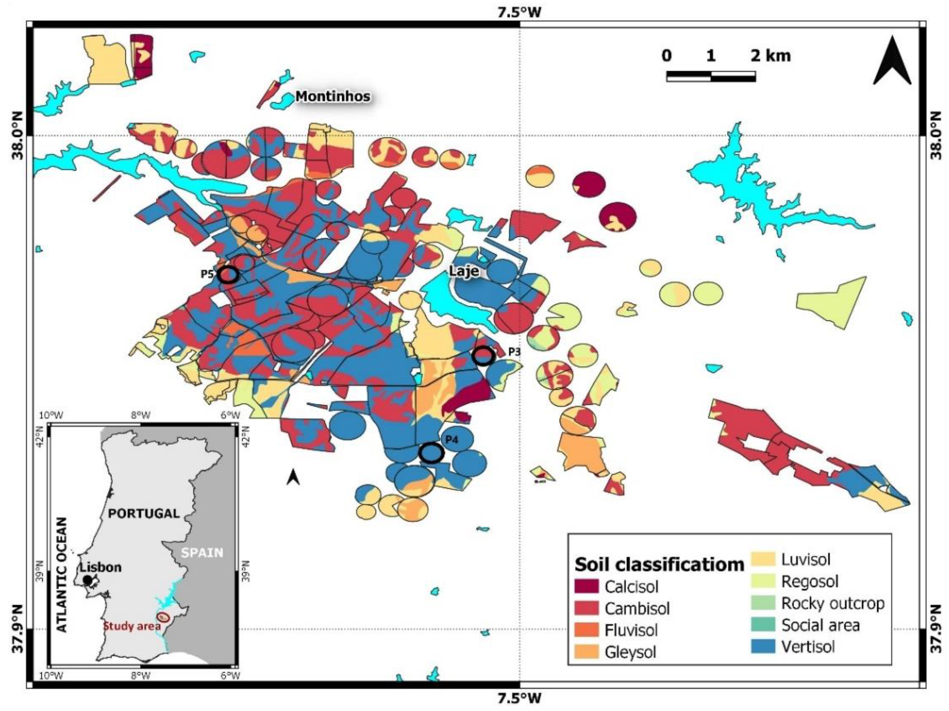
2.1. Study Area

A short-term on-farm study was carried out over three years (2018 to 2020) in three fields of annual crops irrigated by center-pivot, named Pivot 3 (P3), Pivot 4 (P4), and Pivot 5 (P5). In P3, with an area of 13.1 ha, the crop succession throughout the three years was sunflower (Helianthus annus L.), maize (Zea mays L.), and sunflower; in P4, 15.0 ha, the crops were sunflower, arrowleaf clover (Trifolium vesiculosum Savi) for seed production, and onion (Allium cepa L.); the crops in P5, with 10.3 ha, were maize, sunflower, and maize. The fields were located in the Brinches-Enxoé hydro-agricultural area (HAA) with 5061 ha (Figure 1), which is one of the 21 areas of the Alqueva irrigation plan, part of the Multipurpose Development of Alqueva (EFMA—Empreendimento de Fins Múltiplos de Alqueva), centered in the Alqueva reservoir, Guadiana River Basin, southern Portugal. The HAA of Brinches-Enxoé has both pressurized and gravity conveyance networks, with origins in the Laje reservoir and in the Montinhos reservoir, respectively.

The climate in the region is temperate with hot and dry summers (Mediterranean), with an annual precipitation and average mean monthly temperature of, respectively, 558 mm and 16.9 °C (long-term means for the 1981–2010 period, [20]). During the three years of study (2018–2020), data from an automatic meteorological station (37.96833° N; 7.55083° W) located in the HAA, showed that the annual precipitation was 603 mm, 343 mm, and 615 mm, respectively. The mean temperature was 16.7 °C, 17.3 °C, and 17.8 °C, respectively, in 2018, 2019, and 2020 [21]. Predominant soils in P3 and P5 are Calcaric Cambissols and Chromic Vertissols, while in P4 soils are mainly Pelic Vertisols and Calcaric Vertisols [22].

Figure 1. Hydro-agricultural area (HAA) of Brinches-Enxoé, prevalent reference soil groups, and location of the farm plots under study (P3, P4, and P5, marked with bold black circles). The bottom-left inset shows the location of the HAA in southern Portugal (adapted from [23]).

Figure 1. Hydro-agricultural area (HAA) of Brinches-Enxoé, prevalent reference soil groups, and location of the farm plots under study (P3, P4, and P5, marked with bold black circles). The bottom-left inset shows the location of the HAA in southern Portugal (adapted from [23]).

Management practices data were provided by the farmers and are described in

Table 1. Main crop management data in each year (2018 to 2020) and field (P3, P4, and P5) (information provided by the farmers).

Year	Field	Crop	Sowing (dd/mm)	Seasonal Irrigation Water (m3 ha−1)	First Irrigation (dd/mm)	Last Irrigation (dd/mm)	Fertilizer N (kg N ha−1)	Fertilizer P (kg P2O5 ha−1)	Fertilizer K (kg K2O ha−1)	Other Fertilizers (kg ha−1)	Pesticides (Active Substance)	Harvest (dd/mm)	Yield (kg ha−1)
2018	P3	Sunflower	18/04	2517	19/04	01/08	127	34	-	16 SO3; 0.2 B	pre-emergence herbicide (pendimethalin); insecticide (deltamethrin)	27/08	3470
	P4	Sunflower	27/04	4606	28/04	26/08	109	40	12	16 SO3	pre-emergence herbicide (pendimethalin)	18/09	4156
	P5	Maize	18/07	4800	18/07	04/10	202	144	216	27 SO3	post-emergence herbicide (foramsulfuron + isoxadifen-ethyl)	17/01 1	5500
2019	P3	Maize	13/06	7500	2	2	253	-	-	-	post-emergence herbicide (mesotrione + S-metolachlor + terbuthylazine); insecticide (lambda-cyhalothrin)	17/11	11000
	P4	Clover	03/01	1510	18/04	24/06	-	88	-	0.2 SO3; 0.2 B; 0.1 MgO	-	18/09	1703
	P5	Sunflower	16/05	3570	20/05	30/08	81	19	20	7 SO3	pre-emergence herbicides (pendimethalin, glyphosate)	15/09	3257
2020	P3	Sunflower	09/03	5420	2	2	2	2	2	2	2	13/08	8660
	P4	Onion	11/01	3210	11/01	24/08	113	1	0.1	210 SO3; 65 CaO; 2 Zn; 1 Mn; 0.1 MgO	pre- and post-emergence herbicides (aclonifen, clethodime)	21/08	26,848
	P5	Maize	15/06	5160	15/06	15/09	82	59	121	5 SO3; 3 Zn	pre- and post-emergence herbicides (glyphosate, MCPA, 2,4-D + florasulam, mesotrione + S-metolachlor + terbuthylazine); insecticides (lambda-cyhalothrin, chlorantraniliprole)	15/10	9182

¹ Delayed harvest due to the occurrence of a long rainy period following the physiological maturity stage; ^2. No data available (the plot was leased in 2019 and 2020)—no application.

. The soils of the studied fields were conventionally tilled. The fertilizers used were primarily formulations of Nitrogen (NO₃⁻, NH₄⁺, urea), Phosphorus (P₂O₅), and Potassium (K₂O), applied at sowing. Water-soluble and liquid fertilizers, applied over the crops’ cycle through irrigation water, were mostly nitrogen fertilizers but also included other fertilizers containing formulations of sulfur (SO₃), iron (Fe chelates), or calcium (CaO). Foliar applications, containing boron (B), zinc (Zn), magnesium (MgO), and/or manganese (Mn), were employed in some of the crops. The pesticides used were mainly herbicides, but some insecticides were also applied in the sunflower and maize crops.

2.2. Sampling and Data Collection

Soil sampling was carried out on 5 dates (T1 to T5), over the 3 years under study: T1 and T2, in 2018; T3 and T4, in 2019; and T5 in 2020. T1 and T3 took place in spring (March/April); T2, T4, and T5 were carried out at the end of the irrigation period (September/October). The sampling methodology consisted of collecting a composite sample using an open-end soil probe, of every 5-ha area, attending also to surface heterogeneity whenever variations in soil color or slope were observed. Samples were collected in two layers, 0–20 cm and 20–40 cm, obtained from a mixture of approximately 5 sub-samples collected at randomly selected points following a zig-zag trajectory [24]. Samples were then air-dried and sieved with a 2 mm mesh for analysis of the following physical–chemical properties in the <2 mm fraction: particle size distribution (coarse sand (C. Sand), fine sand (F. Sand), Silt and Clay; g kg⁻¹), following ISO 11277:2020 (ISO, 2020); cation exchange capacity (CEC), exchangeable calcium (Ca), magnesium (Mg), potassium (K), sodium (Na), and aluminum (Al) (cmol (+) kg⁻¹), following ISO 11260:2018 (ISO, 2018); pH (H₂O 1:2.5 (p/v)); electrical conductivity of the saturated soil extract (EC; dS m⁻¹) (H₂O 1:2 (p/v)); soil organic matter (SOM; g kg⁻¹), following the Walkley–Black method [25]; total nitrogen (N; %), determined by the Kjeldahl method [26]; available P (mg P₂O₅ kg⁻¹) and K (mg K₂O kg⁻¹), determined by the Egner–Rhiem method [27]. Particle size distribution, exchange cations, and CEC were obtained only in the first sampling (T1) for the initial characterization of the fields. The resulting data matrix consisted of 11 observed variables of 226 composite soil samples.

2.3. Statistical Analysis

Data analyses were performed with Statistica 7 [28] and were conducted separately for each layer. Matrices of Spearman’s correlation coefficients were computed for a preliminary examination of the relationships between the observed soil variables. The FA, using standardized data ((raw value-mean)/standard deviation), was performed to explore the data structure and to reduce the observed variables correlated with each other to a smaller number of independent variables, named factors [11]. Factors were extracted by the PCA method, and the factor loading matrix was subjected to varimax rotation to produce a factor structure that was simpler to interpret [29]. Factors were retained when presenting eigenvalues > 1, a contribution for the proportion of variance > 10%, and at least two observed variables contributing to absolute factor loadings > 0.50 [10,29,30]. Following the methodology reported in Shukla et al. (2006) [18], the scores of the factor models obtained were used to conduct a DA to differentiate sampling dates and fields based on soil attributes, determining which factor, date, or site most contributed to this differentiation. Factors presenting the lowest significant partial Wilks’ Lambda were selected as the dominant discriminant factors [31]. To analyze in detail how each factor may have influenced the temporal and spatial discrimination, a Canonical Analysis (CCA) was carried out, and canonical roots, or discriminant functions, were obtained. The standardized coefficients of the first discriminant function, that is, the one that explains the largest proportion of the model’s variance [31], were selected to verify the weight of each factor in the temporal and spatial discrimination. Finally, having found the preponderant factor for spatial and temporal variability in each soil layer, subsequent Discriminant and Canonical analyses were performed with the original standardized variables, which were highly correlated with each factor, thereby, distinguishing which variable had the greatest influence on the spatial and temporal discrimination of soil attributes and exploring its relationship with the agronomical practices.

3. Results and Discussion

3.1. Soil Physical–Chemical Properties

Overall, soils in the studied sites were rich in clay with medium to fine textures (

Table 2. Average values (± standard error) of particle size fractions (coarse (C) sand, fine (F) sand, Silt, and Clay) and Cation Exchange Capacity (CEC) in each site ((P3 (n = 9), P4 (n = 9), P5 (n = 12)), in the 0–20 cm layer.

Site	C. Sand (g kg−1)	F. Sand (g kg−1)	Silt (g kg−1)	Clay (g kg−1)	CEC (cmol (+) kg−1)
P3	197.6 (±10.0)	230.7 (±6.0)	192.1 (±15.5)	379.6 (±1.8)	56.5 (±0.3)
P4	160.5 (±11.1)	159.2 (±6.5)	248.3 (±1.4)	432.0 (±16.1)	57.0 (±0.8)
P5	163.7 (±9.8)	177.5 (±14.2)	287.6 (±19.1)	371.2 (±25.9)	53.6 (±2.1)

P3—Pivot 3; P4—Pivot 4; P5—Pivot 5; C. Sand—Coarse sand; F. Sand—Fine sand; CEC—Cation Exchange Capacity.

and

Table 3. Average values (± standard error) of particle size fractions (coarse (C) sand, fine (F) sand, Silt, and Clay) and Cation Exchange Capacity (CEC) in each site (P3 (n = 9), P4 (n = 9), P5 (n = 12)), in the 20–40 cm layer.

Site	C. Sand (g kg−1)	F. Sand (g kg−1)	Silt (g kg−1)	Clay (g kg−1)	CEC (cmol (+) kg−1)
P3	192.2 (±11.00)	232.4 (±5.6)	192.7 (±15.7)	375.7 (±2.3)	58.1 (±0.6)
P4	164.1 (±19.08)	167.2 (±6.4)	246.7 (±9.5)	422.0 (±17.0)	57.9 (±1.2)
P5	176.0 (±9.82)	173.3 (±12.6)	243.8 (±5.8)	406.9 (±17.4)	53.9 (±1.4)

P3—Pivot 3; P4—Pivot 4; P5—Pivot 5; C. Sand—Coarse sand; F. Sand—Fine sand; CEC—Cation Exchange Capacity.

). In P3, the soils presented, in both layers, a clay-loam texture; in P4, textures varied from clay-loam to silty-clay; in P5, texture was mainly silty-clay, but there was some spatial variability, with textures also varying from loam to clay-loam and silty-clay-loam. The CEC was very high in every site, in accordance with the clayey nature of these soils and the richness in smectites, characteristic of Vertisols [24,32,33].

The measured soil chemical properties evaluated throughout the study showed a non-saline condition of the soils, in both layers, at every date (

Table 4. Average values (± standard error) of soil chemical parameters in each site (P3 (n = 9), P4 (n = 9), P5 (n = 12)), in the 0–20 cm layer, during the study (T1, T2, T3, T4, and T5 sampling dates).

Date	Site	pH	EC (dS m−1)	SOM (g kg−1)	N (%)	P (mg P2O5 kg−1)	K (mg K2O kg−1)
T1	P3	8.39 (±0.03)	0.16 (±0.00)	15.8 (±0.5)	0.08 (±0.00)	248.61 (±31.32)	115.07 (±9.21)
	P4	8.28 (±0.06)	0.13 (±0.00)	12.8 (±0.4)	0.06 (±0.00)	221.34 (±19.07)	206.59 (±14.06)
	P5	8.02 (±0.03)	0.18 (±0.01)	11.4 (±0.6)	0.08 (±0.00)	418.63 (±88.63)	236.78 (±14.02)
T2	P3	8.34 (±0.03)	0.35 (±0.01)	12.2 (±0.6)	0.09 (±0.00)	124.46 (±17.60)	106.57 (±7.30)
	P4	7.89 (±0.03)	0.35 (±0.02)	19.6 (±2.4)	0.07 (±0.00)	143.64 (±10.22)	149.26 (±4.68)
	P5	8.45 (±0.02)	0.24 (±0.01)	19.1 (±1.8)	0.08 (±0.01)	326.53 (±32.45)	367.04 (±16.31)
T3	P3	8.40 (±0.01)	0.28 (±0.02)	10.6 (±0.8)	0.09 (±0.00)	145.24 (±12.73)	102.62 (±13.52)
	P4	1
	P5	1
T4	P3	8.08 (±0.02)	0.29 (±0.01)	10.0 (±0.4)	0.10 (±0.00)	148.57 (±14.68)	94.98 (±6.93)
	P4	8.25 (±0.02)	0.26 (±0.01)	6.9 (±0.4)	0.08 (±0.00)	115.81 (±6.99)	145.16 (±5.96)
	P5	8.06 (±0.04)	0.30 (±0.01)	16.0 (±0.6)	0.10 (±0.00)	239.86 (±21.76)	226.06 (±14.34)
T5	P3	7.92 (±0.01)	0.58 (±0.01)	15.0 (±0.2)	0.10 (±0.00)	180.82 (±18.98)	147.75 (±18.55)
	P4	7.80 (±0.01)	0.46 (±0.02)	10.4 (±0.2)	0.09 (±0.01)	106.32 (±6.64)	261.43 (±48.24)
	P5	1

¹ No data available (samples were not collected). P3—Pivot 3; P4—Pivot 4; P5—Pivot 5. EC—Electrical Conductivity; SOM—Soil Organic Matter; N—Nitrogen; P—Phosphorus; K—Potassium.

and

Table 5. Average values (± standard error) of soil chemical parameters in each site (P3 (n = 9), P4 (n = 9), P5 (n = 12)), in the 20–40 cm layer, during the study (T1, T2, T3, T4, and T5 sampling dates).

Date	Site	pH	EC (dS m−1)	SOM (g kg−1)	N (%)	P (mg P2O5 kg−1)	K (mg K2O kg−1)
T1	P3	8.49 (±0.02)	0.15 (±0.00)	16.9 (±1.4)	0.07 (±0.00)	144.85 (±7.02)	94.82 (±7.05)
	P4	8.19 (±0.05)	0.16 (±0.00)	8.2 (±0.2)	0.05 (±0.00)	131.13 (±4.44)	139.03 (±3.62)
	P5	8.09 (±0.07)	0.14 (±0.01)	7.9 (±0.6)	0.06 (±0.00)	258.99 (±67.76)	150.23 (±11.43)
T2	P3	8.40 (±0.03)	0.30 (±0.02)	11.2 (±0.4)	0.08 (±0.00)	106.20 (±15.77)	96.99 (±6.14)
	P4	7.97 (±0.02)	0.29 (±0.02)	18.5 (±3.1)	0.07 (±0.00)	83.74 (±1.71)	139.38 (±3.09)
	P5	8.49 (±0.02)	0.30 (±0.02)	16.8 (±1.5)	0.07 (±0.00)	197.73 (±18.97)	183.27 (±9.77)
T3	P3	8.35 (±0.02)	0.29 (±0.01)	10.2 (±0.9)	0.08 (±0.01)	148.44 (±12.28)	121.46 (±19.84)
	P4	1
	P5	1
T4	P3	8.10 (±0.01)	0.32 (±0.01)	9.8 (±0.8)	0.10 (±0.00)	118.42 (±11.96)	86.27 (±7.98)
	P4	1
	P5	7.98 (±0.01)	0.37 (±0.01)	15.1 (±0.8)	0.09 (±0.00)	192.95 (±16.97)	195.35 (±16.83)
T5	P3	8.11 (±0.01)	0.28 (±0.00)	13.3 (±0.4)	0.09 (±0.00)	133.02 (±14.65)	73.48 (±9.30)
	P4	7.83 (±0.05)	0.41 (±0.04)	9.0 (±0.4)	0.09 (±0.01)	74.64 (±4.27)	164.78 (±11.08)
	P5	1

¹ No data available (samples were not collected). P3—Pivot 3; P4—Pivot 4; P5—Pivot 5. EC—Electrical Conductivity; SOM—Soil Organic Matter; N—Nitrogen; P—Phosphorus; K—Potassium.

). Soils in the superficial layer (0–20 cm) presented a slight to medium alkaline reaction due to their calcareous nature, with average pH values in the range of 7.8–8.5 [32]. The alkaline nature of these soils is associated with deficiencies in nutrients such as Zn, Cu, Fe, Mn, and B, which are especially common in irrigated crops [34]; hence, it is common to apply these nutrients, either in the form of chelates (in the case of iron) or by using foliar applications of Zn, Mn, and B, practices that were adopted by the farmers, as reported in Section 2.1. The studied soils presented low levels of SOM, a feature of regions in arid or semi-arid climates, and reduced values of total N, in accordance with their low organic content, which increases the fertilization rates required to meet the crops’ extraction. Available P presented high to very high levels, especially in P5 at T1. The same occurs regarding the levels of available K. The values at different dates point to a decreasing trend in P₂O₅ and K₂O between the beginning (T1, T3, T5) and the end (T2, T4) of the crops’ cycle/irrigation season, which could be a result of the nutrient’s extraction by the plants or, in the case of P, of the possible formation of insoluble calcium-phosphate compounds (P fixation), a common occurrence in soils with abundant Ca²⁺ or Mg²⁺ [34]. However, the levels of these nutrients remaining in the soil at the end of the crops’ cycle was still high or very high. The fixation of P added by fertilization results in low uptake during the year of application and, normally, only approximately 10% to 20% of applied P is used by the plants during the first year. Therefore, the repeated application of P by fertilization leads to soils becoming sufficiently high in this nutrient [32]. This buildup of the available P in soils to levels beyond the amounts required by the crops means that these high amounts of the element are prone to leaching and can contribute to eutrophication processes [15].

The maintenance of high solution potassium concentrations is determined by the K buffer capacity of the soil, which is high in the case of fine-textured soils containing abundant vermiculite and ilite clay minerals, with large amounts of interlayer K. In these soils, with high K-fixing capacity, much of the K applied by fertilization would be lost to fixation but, in the absence of easily supplied fertilizer K, a significant portion of K required by plants comes from the interlayer K, which is indicative of the beneficial role of the fixed K [35].

From the 0–20 cm to the sub-superficial layer (20–40 cm), the values of available P and K decrease, showing that both the application of fertilizers and the nutrient uptake by plants occurs mainly in the surface layer, where roots are more active (Table 5).

3.2. Correlation and Data Structure

3.2.1. Layer 0–20 cm

The Spearman correlation coefficients between the 11 soil physical–chemical parameters, measured in the 0–20 cm layer, can be observed in

Table 6. Spearman correlation matrix of soil physical–chemical parameters in the 0–20 cm layer.

	pH	EC	SOM	N	P	K	C. Sand	F. Sand	Silt	Clay	CEC
pH	1.000
EC	−0.487	1.000
SOM	0.093	0.011	1.000
N	−0.270	0.591	0.150	1.000
P	0.273	−0.461	0.426	0.021	1.000
K	−0.108	−0.124	0.348	0.020	0.538	1.000
C. Sand	0.068	0.050	−0.075	0.047	−0.162	−0.449	1.000
F. Sand	0.103	0.108	−0.025	0.178	−0.119	−0.441	0.920	1.000
Silt	−0.078	−0.117	0.198	−0.030	0.119	0.447	−0.556	−0.396	1.000
Clay	−0.123	0.086	−0.180	−0.086	0.088	0.155	−0.554	−0.564	−0.197	1.000
CEC	−0.170	0.164	−0.245	0.043	−0.196	−0.151	−0.033	−0.097	−0.302	0.434	1.000

Bold values are significant at p < 0.05. EC—Electrical Conductivity; SOM—Soil Organic Matter; N—Nitrogen; P—Phosphorus; K—Potassium; C. Sand—Coarse sand; F. Sand—Fine sand; CEC—Cation Exchange Capacity.

. Significant moderate positive correlations (>0.40) were found between EC and N, SOM and P, P and K, K and silt, clay and CEC. Significant negative correlations <−0.40 were observed between pH and EC, EC and P, K and sand fractions.

The FA performed for the 0–20 cm layer allowed for the extraction of four factors, accounting for 75.04% of the total variance in the dataset (

Table 7. Factor loadings, eigenvalues, percentage of total variance, and accumulated variance, in a four-factor model of 11 observed soil variables in the 0–20 cm layer.

	Factor 1	Factor 2	Factor 3	Factor 4
pH	0.215	0.043	−0.719	−0.186
EC	0.093	0.111	0.893	0.070
SOM	−0.061	−0.195	0.100	−0.542
N	0.198	0.035	0.753	−0.251
P	0.015	0.068	−0.257	−0.799
K	−0.323	−0.092	0.073	−0.741
C. Sand	0.897	−0.259	0.004	0.152
F. Sand	0.943	−0.256	0.053	0.100
Silt	−0.793	−0.527	−0.042	−0.169
Clay	−0.413	0.861	0.001	0.008
CEC	0.008	0.830	0.088	0.183
Eigenvalues	2.988	2.224	1.837	1.206
% Total variance	27.16	20.22	16.70	10.97
%. Accumulated variance	27.16	47.38	64.08	75.04

Bold values correspond to the higher factor loadings (>0.50) of the variables in each factor. EC—Electrical Conductivity; SOM—Soil Organic Matter; N—Nitrogen; P—Phosphorus; K—Potassium; C. Sand—Coarse sand; F. Sand—Fine sand; CEC—Cation Exchange Capacity.

).

Factor 1 accounted for 27.16% of the total variance and presented factor loadings with absolute values > 0.50 for C. Sand (0.897), F. Sand (0.943), and Silt (−0.793), indicating it was a factor translating the attribute texture. Factor 2 (20.22% of total variance) presented high positive loadings of the variables Clay (0.861) and CEC (0.830), thereby being a factor that characterized water and nutrients retention capacity. Factor 3 described 16.70% of the models’ variance and was highly correlated with pH (−0.719), EC (0.893), and N (0.753), therefore representing an attribute of chemical composition. Factor 4, accounting for 10.97% of total variance, was related to fertility, because it was highly correlated with SOM (−0.542), available P (−0.799), and available K (−0.741).

3.2.2. Layer 20–40 cm

Correlation coefficients between chemical parameters in the sub-surface layer were lower than the ones obtained for the superficial layer, probably resulting from an attenuation of the influence of agronomical practices, such as tillage or fertilization, with increasing depth (

Table 8. Spearman correlation matrix of soil physical–chemical parameters in the 20–40 cm layer.

	pH	EC	SOM	N	P	K	C. Sand	F. Sand	Silt	Clay	CEC
pH	1.000
EC	−0.301	1.000
SOM	0.234	0.124	1.000
N	−0.172	0.672	0.326	1.000
P	0.397	−0.111	0.224	−0.042	1.000
K	−0.232	0.209	0.183	−0.036	0.302	1.000
C. Sand	0.019	0.092	0.135	0.054	0.082	−0.073	1.000
F. Sand	0.266	0.001	0.062	0.176	−0.013	−0.541	0.712	1.000
Silt	−0.181	−0.064	−0.065	−0.118	−0.105	0.405	−0.868	−0.820	1.000
Clay	−0.130	−0.022	−0.120	−0.157	0.103	0.286	−0.800	−0.894	0.691	1.000
CEC	−0.026	−0.147	−0.178	−0.023	−0.134	−0.190	−0.517	−0.121	0.278	0.289	1.000

Bold values are significant at p < 0.05. EC—Electrical Conductivity; SOM—Soil Organic Matter; N—Nitrogen; P—Phosphorus; K—Potassium; C. Sand—Coarse sand; F. Sand—Fine sand; CEC—Cation Exchange Capacity.

). Moderate absolute correlations (>0.40) were found only between EC and N and K, F. Sand, and Silt. Regarding physical–chemical characteristics, high positive correlations were found between coarser (fine and coarse sand) and smaller separates (silt and clay). A correlation coefficient of −0.517 was found between C. Sand and CEC.

In the 20–40 cm layer, the FA retained four factors responsible for 75.72% of the total variance, with a structure similar to the model found for the surface layer (

Table 9. Factor loadings, eigenvalues, percentage of total variance, and accumulated variance, in a four-factor model of 11 observed soil variables in the 20–40 cm layer.

	Factor 1	Factor 2	Factor 3	Factor 4
pH	0.195	−0.288	0.241	0.752
EC	0.038	0.863	−0.148	−0.200
SOM	0.063	0.363	−0.092	0.562
N	0.032	0.894	0.124	0.066
P	−0.141	−0.211	−0.443	0.594
K	−0.464	0.233	−0.695	0.228
C. Sand	0.929	0.024	−0.275	0.005
F. Sand	0.925	0.041	0.237	0.085
Silt	−0.869	−0.007	−0.099	−0.050
Clay	−0.869	−0.052	0.127	−0.034
CEC	−0.302	0.043	0.758	0.094
Eigenvalues	3.614	1.953	1.611	1.152
% Total variance	32.85	17.75	14.65	10.47
%. Accumulated variance	32.85	50.60	65.25	75.72

Bold values correspond to the higher factor loadings (>0.50) of the variables in each factor. EC—Electrical Conductivity; SOM—Soil Organic Matter; N—Nitrogen; P—Phosphorus; K—Potassium; C. Sand—Coarse sand; F. Sand—Fine sand; CEC—Cation Exchange Capacity.

). Factor 1 accounted for 32.85% of total variance and presented absolute loads > 0.50 of the particle size variables—C. Sand (0.929), F. Sand (0.925), Silt (−0.869), and Clay (−0.869)—therefore, it was a proxy of soil texture. Factor 2, representing 17.75% of total variance of the model, presented high positive loads of EC (0.863) and N (0.894), hence being related to chemical composition. Factor 3 (14.65% of total variance) was highly positively correlated with CEC (0.758) and negatively correlated with available K (−0.695); therefore, we considered it as essentially representative of a nutrient availability attribute. Factor 4 (10.47% of total variance) showed high factor loadings of pH (0.752), SOM (0.562), and available P (0.594) and was thereby named a fertility attribute.

3.3. Discriminant Factors and Variables

3.3.1. Layer 0–20 cm

The DA performed with the factor scores of cases obtained for the 0–20 cm layer indicated that Factor 3, with the lowest significant partial Wilks’ Lambda of 0.597 (p < 0.001) was the most influent factor for temporal variability (sampling dates). Therefore, the differences in soil surface samples over time were predominantly affected by variations in the chemical composition, namely, by pH, EC, and N. Factor 1, showing the lowest significant partial Wilks’ Lambda of 0.648, was the dominant factor for spatial variability (fields) (p < 0.001). Therefore, it was the texture attribute that most contributed to the spatial differentiation in the soil surface.

The first discriminant functions (roots) for factors (Y) considering time (sampling dates) and space (crop fields), and their respective factor coefficients obtained with the CCA for the surface layer confirmed the previous DA: higher absolute roots were obtained for Factor 3 and Factor 1, respectively, in temporal and spatial discrimination ((Equations (1) and (2)). The discriminant functions found accounted for 71.03% and 85.52% of the total variance ((respectively, Equations (1) and (2)):

Temporal variability:

Y_T = −0.252 (Factor 1) − 0.175 (Factor 2) + 0.973 (Factor 3) − 0.170 (Factor 4),

(1)

Spatial variability:

Y_S = −1.941 (Factor 1) − 0.563 (Factor 2) + 0.062 (Factor 3) − 0.054 (Factor 4),

(2)

The DA and CCA performed with the variables highly correlated with the dominant factors in the temporal and spatial variability allowed us to find the following first discriminant functions for the variables (Y′), accounting, respectively, for 86.50% and 92.89% of the total variance (Equations (3) and (4), respectively):

Temporal variability:

Y′_T = 0.130 (pH) + 1.220 (EC) − 0.462 (N),

(3)

Spatial variability:

Y′_S = −0.469 (C. Sand) + 1.886 (F. Sand) − 0.368 (Silt),

(4)

Considering the standardized coefficients of each variable, the differences over time in soil surface were predominantly identified by EC, available N, and pH. These results may be indicative of seasonal changes in soil salinity due to irrigation water quality degradation [23,36], along with the influence of fertilization and fertigation, whose management deserves attention in order to avoid salinization or N losses to the environment through leaching, ammonia (NH₃) volatilization, or bacterial denitrification of nitrate (NO₃-N) [37]. Fine sand proportion was the variable that mostly influenced the spatial variation, followed by Coarse sand and Silt proportions.

3.3.2. Layer 20–40 cm

In the case of the sub-surface layer, the DA revealed a preponderance of Factor 2 (chemical composition) and Factor 3 (nutrient availability) in temporal (partial Wilks’ Lambda of 0.358; p < 0.001) and spatial (partial Wilks’ Lambda of 0.532; p < 0.001) discrimination, respectively. The discriminant functions considering temporal and spatial variation (Y_T and Y_S, respectively) accounted for 79.39% and 97.92% of total variance and presented the coefficients presented in Equations (5) and (6), respectively:

Temporal variability:

Y_T = 0.284 (Factor 1) − 1.012 (Factor 2) − 0.319 (Factor 3) + 0.081 (Factor 4),

(5)

Spatial variability:

Y_S = 0.719 (Factor 1) + 0.284 (Factor 2) + 0.964 (Factor 3) + 0.554 (Factor 4),

(6)

The coefficients of each factor confirm that the chemical composition attribute (Factor 3 and Factor 2, in each layer, respectively) is the one that had the most influence on temporal differentiation, denoting the influence of crop management, e.g., fertilization and irrigation, or, indirectly, of the soil organic content, through the variable N total [18,38].

While texture (Factor 1) was predominant in the differentiation between fields, in the case of the surface layer, in the sub-surface layer this differentiation was mostly influenced by the nutrient availability (Factor 3). These results point to the importance of the soil particle distribution, the presence of clay and its close relationship with CEC, and the high to very high levels of available K found throughout the study, for the spatial variability.

The first discriminant functions for the variables highly correlated with the identified factors (Y′), accounting, respectively, for 84.63% and 80.96% of the total variance, are presented in Equations (7) and (8):

Temporal variability:

Y′_T = −0.741 (EC) − 0.502 (N),

(7)

Spatial variability:

Y′_S = −0.904 (K) + 0.607 (CEC),

(8)

In both layers, EC is the soil parameter that most contributes to the variability that occurs over time, followed by N total. As usual, nitrogen fertilization rates were higher than any of the other applied nutrients in every field and year, except for 2020, where 350 kg ha⁻¹ of ammonium sulfate (20.5% N + 60% SO₃) was applied in the onion crop, significantly increasing the amount of sulfur applied compared to any other nutrient in the P4 field. Moreover, N is employed not only at sowing, but also in top dressing fertilizations, and in soluble formulations applied with irrigation during the crop development. Therefore, the influence of N in temporal discrimination was expected, and specific consideration should be taken regarding N fertilization management. The importance of EC is linked not only with irrigation water quality, but also with the correlation between this parameter and many of the main physicochemical properties of the soil, such as proportion of clay, soil water content, soil bulk density, and soil organic content, which are subject to spatial and temporal changes in agricultural soils. In fact, this correlation is the basis for the use of soil apparent electrical conductivity measured by expeditious methods in distinguishing agronomic management zones and productivity maps, presently, with widespread application in precision agriculture [39,40,41].

4. Conclusions

The integrated knowledge of the temporal and spatial variation of soil properties can improve crop productivity and prevent soil degradation. Given the multidimensional and multivariate nature of soil sampling data, the use of multivariate statistical analysis tools may help to better understand the dynamics of variation in time and space and the relationships between agronomic parameters and soil functions. The Factor Analysis performed with data collected in three fields of irrigated annual crops during the period 2018–2020, in two soil layers (0–20 cm and 20–40 cm) allowed us to obtain two models of four factors for each layer. The model obtained for the surface layer included factors related to the attributes texture, water and nutrient retention capacity, chemical composition, and soil fertility. In the sub-surface layer, the model of factor structure was similar. The most influential factor in temporal discrimination (sampling dates) was related to chemical composition, indicating the influence of crop management practices such as fertilization and irrigation. As for the spatial differentiation (fields), the dominant factor in the surface layer was texture, and in the sub-surface layer, nutrient availability. The variable most influent in temporal discrimination in both the surface and sub-surface layers was EC. The most preponderant spatial discriminant variables were fine sand proportion and available potassium in the 0–20 cm layer and 20–40 cm layer, respectively. Further studies on this subject should consider the integration of biological and ecotoxicological indicators as soil health indicators to attend to the intensification in the use of fertilizers and plant protection products in irrigated agriculture, thereby understanding better the implications of larger inputs of these products on the sustainability of irrigated soils.

References

1. Adhikari, K.; Hartemink, A.E. Linking Soils to Ecosystem Services—A Global Review. Geoderma 2016, 262, 101–111. [Google Scholar] [CrossRef]
2. Larson, W.E.; Pierce, F.J. The Dynamics of Soil Quality as a Measure of Sustainable Management. In Defining Soil Quality for a Sustainable Environment; Doran, J.W., Coleman, D.C., Bezdicek, D.F., Stewart, B.A., Eds.; SSSA Special Publication Number: Wisconsin, WI, USA, 1994; pp. 37–51. [Google Scholar]
3. Karlen, D.L.; Veum, K.S.; Sudduth, K.A.; Obrycki, J.F.; Nunes, M.R. Soil Health Assessment: Past Accomplishments, Current Activities, and Future Opportunities. Soil Tillage Res. 2019, 195, 104365. [Google Scholar] [CrossRef]
4. FAO Water. Key Facts. Available online: http://www.fao.org/water/en/ (accessed on 27 September 2021).
5. Adejumobi, M.A.; Awe, G.O.; Abegunrin, T.P.; Oyetunji, O.M.; Kareem, T.S. Effect of Irrigation on Soil Health: A Case Study of the Ikere Irrigation Project in Oyo State, Southwest Nigeria. Environ. Monit. Assess. 2016, 188, 696. [Google Scholar] [CrossRef] [PubMed]
6. Nikolskii, Y.; Aidarov, I.P.; Landeros-Sanchez, C.; Pchyolkin, V.V. Impact of Long-Term Freshwater Irrigation on Soil Fertility. Irrig. Drain. 2019, 68, 993–1001. [Google Scholar] [CrossRef]
7. Bendra, B.; Fetouani, S.; Laffray, X.; Vanclooster, M.; Sbaa, M.; Aleya, L. Effects of Irrigation on Soil Physico-Chemistry: A Case Study of the Triffa Plain (Morocco). Irrig. Drain. 2012, 61, 507. [Google Scholar] [CrossRef]
8. Murray, R.S.; Grant, C.D. The impact of irrigation on soil structure. Land & Water Australia; Land & Water Australia: Camberra, Australia, 2007; p. 31. Available online: https://library.dbca.wa.gov.au/static/FullTextFiles/070521.pdf (accessed on 27 September 2021).
9. Presley, D.R.; Ransom, M.D.; Kluitenberg, G.J.; Finnell, P.R. Effects of Thirty Years of Irrigation on the Genesis and Morphology of Two Semiarid Soils in Kansas. Soil Sci. Soc. Am. J. 2004, 68, 1916–1926. [Google Scholar] [CrossRef]
10. Jagadamma, S.; Lal, R.; Hoeft, R.G.; Nafziger, E.D.; Adee, E.A. Nitrogen Fertilization and Cropping System Impacts on Soil Properties and Their Relationship to Crop Yield in the Central Corn Belt, USA. Soil Tillage Res. 2008, 98, 120–129. [Google Scholar] [CrossRef]
11. Härdle, W.K.; Simar, L. Applied Multivariate Statistical Analysis, 4th ed.; Springer: Heidelberg, NY, USA; Dordrecht, The Netherlands; London, UK, 2015; ISBN 978-3-662-45171-7. [Google Scholar]
12. Yeater, K.; Villamil, M. Multivariate Methods for Agricultural Research. In Applied Statistics in Agricultural, Biological, and Environmental Sciences; Glaz, B., Yeater, K.M., Eds.; American Society of Agronomy, Inc.; Soil Science Society of America, Inc.; Crop Science Society of America, Inc.: Madison, WI, USA, 2018; ISBN 978-0-89118-359-4. [Google Scholar] [CrossRef]
13. Quiroga, A.R.; Buschiazzo, D.E.; Peinemann, N. Management Discriminant Properties in Semiarid Soils. Soil Sci. 1998, 163, 591–597. [Google Scholar] [CrossRef]
14. Sena, M.M.; Frighetto, R.T.S.; Valarini, P.J.; Tokeshi, H.; Poppi, R.J. Discrimination of Management Effects on Soil Parameters by Using Principal Component Analysis: A Multivariate Analysis Case Study. Soil Tillage Res. 2002, 67, 171–181. [Google Scholar] [CrossRef]
15. Preston, W.; Nascimento, C.; Silva, Y.; Silva, D.; Ferreira, H. Soil Fertility Changes in Vineyards of a Semiarid Region in Brazil. J. Soil Sci. Plant Nutr. 2017, 17, 672–685. [Google Scholar] [CrossRef] [Green Version]
16. Mallarino, A.; Oyarzabal, E.; Hinz, P. Interpreting Within-Field Relationships Between Crop Yields and Soil and Plant Variables Using Factor Analysis. Precis. Agric. 1999, 1, 15–25. [Google Scholar] [CrossRef]
17. Juhos, K.; Szabó, S.; Ladányi, M. Influence of Soil Properties on Crop Yield: A Multivariate Statistical Approach. Int. Agrophys. 2015, 29, 433–440. [Google Scholar] [CrossRef]
18. Shukla, M.K.; Lal, R.; Ebinger, M. Determining Soil Quality Indicators by Factor Analysis. Soil Tillage Res. 2006, 87, 194–204. [Google Scholar] [CrossRef]
19. Firdous, S.; Begum, S.; Yasmin, A. Assessment of Soil Quality Parameters Using Multivariate Analysis in the Rawal Lake Watershed. Environ. Monit. Assess. 2016, 188, 533. [Google Scholar] [CrossRef]
20. IPMA Climate normal—1981–2010—Beja. Available online: https://www.ipma.pt/en/oclima/normais.clima/1981-2010/002/ (accessed on 6 July 2022).
21. COTR SAGRA—Sistema Agrometeorológico Para a Gestão Da Rega No Alentejo (Agrometeorological System for Irrigation Management in Alentejo). Available online: http://www.cotr.pt/servicos/sagranet.php (accessed on 15 February 2022).
22. IUSS Working Group WRB World Reference Base for Soil Resources 2014; Update 2015; FAO: Rome, Italy, 2014.
23. Tomaz, A.; Costa, M.J.; Coutinho, J.; Dôres, J.; Catarino, A.; Martins, I.; Mourinha, C.; Guerreiro, I.; Pereira, M.M.; Fabião, M.; et al. Applying Risk Indices to Assess and Manage Soil Salinization and Sodification in Crop Fields within a Mediterranean Hydro-Agricultural Area. Water 2021, 13, 3070. [Google Scholar] [CrossRef]
24. Varennes, A.D. Produtividade Dos Solos e Ambiente (Productivity of Soils and Environment); Escolar Editora: Lisboa, Portugal, 2003. [Google Scholar]
25. Walkley, A.; Black, L.A. An Examination of the Dgtjareff Method for Determining Soil Organic Matter, and a Proposed Modification of the Chromic Acid Titration Method. Soil Sci. 1934, 37, 29–38. [Google Scholar] [CrossRef]
26. Kjeldahl, J. Neue Methode zur Bestimmung des Stickstoffs in organischen Körpern (New method for the determination of nitrogen in organic substances). Z. Für Anal. Chem. 1883, 22, 366–383. [Google Scholar] [CrossRef] [Green Version]
27. Egner, H.; Riehm, H.; Domingo, W.R. Untersuchhungen Uber Die Chemische Boden: Analyse Als Grundlage Fur Die Beurteilung Der Nahrstoffzustandes Der Boden. II. Chemique Extractions, Methoden Zur Phosphor, Und Kalium-Bestimmung (Investiga-Tions on the Chemical Soil Analysis as a Basis for Assess-Ing the Soil Nutrient Status II: Chemical Extractionmethods for Phosphorus and Potassium Determination). K. Lantbr. Ann. 1960, 26, 199–215. [Google Scholar]
28. StatSoft, Inc. STATISTICA (Data Analysis Software System); StatSoft, Inc.: Tulsa, OK, USA, 2004; Available online: https://www.tibco.com/products/tibco-statistica (accessed on 15 February 2022).
29. Tomaz, A.; Palma, J.F.; Ramos, T.; Costa, M.N.; Rosa, E.; Santos, M.; Boteta, L.; Dôres, J.; Patanita, M. Yield, Technological Quality and Water Footprints of Wheat under Mediterranean Climate Conditions: A Field Experiment to Evaluate the Effects of Irrigation and Nitrogen Fertilization Strategies. Agric. Water Manag. 2021, 258, 107214. [Google Scholar] [CrossRef]
30. Lee, K.-M.; Herrman, T.J.; Lingenfelser, J.; Jackson, D.S. Classification and Prediction of Maize Hardness-Associated Properties Using Multivariate Statistical Analyses. J. Cereal Sci. 2005, 41, 85–93. [Google Scholar] [CrossRef]
31. TIBCO TIBCO Statistica® User′s Guide, Version 14.0. Available online: https://docs.tibco.com/pub/stat/14.0.0/doc/html/UsersGuide/GUID-058F49FC-F4EF-4341-96FB-A785C2FA76E9-homepage.html (accessed on 22 April 2020).
32. Foth, H.D. Fundamentals of Soil Science, 8th ed.; John Wiley & Sons, Inc.: New York, NY, USA, 1990; ISBN 0-471-52279-1. [Google Scholar]
33. Parfitt, R.; Giltrap, D.; Whitton, J. Contribution of Organic Matter and Clay Minerals to the Cation Exchange Capacity of Soil. Commun. Soil Sci. Plant Anal. 1995, 26, 1343–1355. [Google Scholar] [CrossRef]
34. Weil, R.R.; Brady, N.C. The Nature and Properties of Soils, 15th ed.; Pearson: Columbus, OH, USA, 2016; ISBN 978-0-13-325448-8. [Google Scholar]
35. Chatterjee, D.; Datta, S.C.; Manjaiah, K.M. Fractions, Uptake and Fixation Capacity of Phosphorus and Potassium in Three Contrasting Soil Orders. J. Soil Sci. Plant Nutr. 2014, 14, 640–656. [Google Scholar] [CrossRef]
36. Tomaz, A.; Palma, P.; Fialho, S.; Lima, A.; Alvarenga, P.; Potes, M.; Costa, M.; Salgado, R. Risk Assessment of Irrigation-Related Soil Salinization and Sodification in Mediterranean Areas. Water 2020, 12, 3569. [Google Scholar] [CrossRef]
37. Sapkota, T.B.; Singh, L.K.; Yadav, A.K.; Khatri-Chhetri, A.; Jat, H.S.; Sharma, P.C.; Jat, M.L.; Stirling, C.M. Identifying Optimum Rates of Fertilizer Nitrogen Application to Maximize Economic Return and Minimize Nitrous Oxide Emission from Rice–Wheat Systems in the Indo-Gangetic Plains of India. Arch. Agron. Soil Sci. 2020, 66, 2039–2054. [Google Scholar] [CrossRef] [Green Version]
38. Simfukwe, P.; Hill, P.W.; Emmett, B.A.; Jones, D.L. Identification and Predictability of Soil Quality Indicators from Conventional Soil and Vegetation Classifications. PLoS ONE 2021, 16, e0248665. [Google Scholar] [CrossRef] [PubMed]
39. Corwin, D.L.; Lesch, S.M. Apparent Soil Electrical Conductivity Measurements in Agriculture. Comput. Electron. Agric. 2005, 46, 11–43. [Google Scholar] [CrossRef]
40. Fortes, R.; Millán, S.; Prieto, M.H.; Campillo, C. A Methodology Based on Apparent Electrical Conductivity and Guided Soil Samples to Improve Irrigation Zoning. Precis. Agric. 2015, 16, 441–454. [Google Scholar] [CrossRef]
41. Moral, F.J.; Terrón, J.M.; Silva, J.R.M. da Delineation of Management Zones Using Mobile Measurements of Soil Apparent Electrical Conductivity and Multivariate Geostatistical Techniques. Soil Tillage Res. 2010, 106, 335–343. [Google Scholar] [CrossRef]