Article

Assessment of Artificial Sweeteners as Wastewater Co-Tracers in an Urban Groundwater System of Mexico (Monterrey Metropolitan Area)

1
Escuela de Ingenieria y Ciencias, Tecnologico de Monterrey, Av. Eugenio Garza Sada Sur N° 2501, Monterrey 64849, Nuevo León, Mexico
2
Escuela de Ingenieria y Ciencias, Tecnologico de Monterrey, Atlixcáyotl 5718, Reserva Territorial Atlixcáyotl, Puebla 72453, Puebla, Mexico
3
Escuela de Ingenieria y Ciencias, Tecnologico de Monterrey, Av. General Ramón Corona #2514, Col. Nuevo México, Zapopan 45138, Jalisco, Mexico
*
Author to whom correspondence should be addressed.
Water 2022, 14(20), 3210; https://doi.org/10.3390/w14203210
Submission received: 23 August 2022 / Revised: 25 September 2022 / Accepted: 29 September 2022 / Published: 12 October 2022

Abstract

:
Contamination from wastewater infiltration, typically from leaky sewers, poses a threat to urban groundwater resources. Artificial sweeteners (Asws), used as sucrose substitutes in many products of daily consumption, are released into groundwater systems and may be used as tracers of wastewater in urban groundwater environments, because most of these compounds are discharged directly into sewer systems. Here, for the first time, we investigated the occurrence of Asws in an urban groundwater system in Mexico. Artificial sweetener concentrations of acesulfame (ACE), aspartame (ASP), cyclamate (CYC), saccharin (SAC), and sucralose (SUC) were tested in 42 production wells in the Monterrey Metropolitan Area (MMA). The detection frequencies of quantified Asws observations were in the order ACE (57%) > SUC (54%) > SAC (7%), with SUC being the most abundant Asws, with concentrations below the quantification limit (BQL) of 2.9 µg/L, followed by ACE (BQL 0.73 µg/L) and SAC (BQL 1.4 µg/L). ASP and CYC were not detected at any sampling site. Considerable Asws ingestion amongst the MMA population is the main input source of Asws into the city’s wastewater network, percolating into the urban groundwater system due to leaky sewers. Our work shows that the application of Asws as wastewater tracers (SUC and ACE) effectively determines wastewater sources affecting urban groundwater.

1. Introduction

Artificial sweeteners have gained popularity as sugar substitutes in low-calorie diets and foods, beverages, pharmaceutical compounds, animal feed additives, and personal care products for more than a decade under the label of “healthy foods” [1,2,3]. Some of the best-known Asws are acesulfame (ACE), aspartame (ASP), cyclamate (CYC), saccharin (SAC), and sucralose (SUC) (Table S1, Supplementary Materials). The occurrence and persistence of Asws in environmental waters have been associated with surface runoff, sewage overflows, landfill leachates, septic spills, septic groundwater plumes, and wastewater effluents from urban water systems [4,5,6,7,8]. The main reason for their occurrence is that after Asws ingestion, the human body does not metabolize them. Therefore, they are disseminated into sewage systems in high quantities. Additionally, these compounds show a low removal efficiency in wastewater treatment plants (WWTPs) and exhibit increased stability and persistence in water [4,6,7,8,9].
Given their persistence in water and wastewater, various attempts have been made over the past decade to evaluate wastewater contamination in groundwater using Asws as tracers [4,5,7,8,10,11]. Several factors that identify Asws as ideal tracers for wastewater impact are as follows: (i) they are source-specific; (ii) they show low WWTP removal efficiency; (iii) their environmental background concentration is zero; (iv) they bear negligible attenuation in receiving water sources; and (v) they are amenable to sensitive analyses capable of detecting concentration changes in receiving waters [4,12,13].
Specifically, ACE and SUC have demonstrated high stability in municipal wastewater effluents [14]. Both sweetening compounds are only partially mineralized through microbial co-metabolism in sediments. In addition, both compounds have shown WWTP removal rates lower than 50%, making them conservative markers of raw and treated wastewater [5,8,15]. Otherwise, CYC and SAC have also been classified as labile markers for raw wastewater pollution in surface waters and groundwater [14,15]. Although they are hydrophilic, they are partially metabolized after ingestion. As a result, much lower concentrations of CYC and SAC in WWTP effluents have been found compared with those of ACE and SUC [4,16]. It has been observed that ACE and SUC serve as good indicators of conventional treated wastewater and septic system pollution in North America, Europe, and Asia [7,17,18,19], whereas both CYC and SAC have failed to be considered as conservative wastewater pollution indicators due to the high wastewater treatment efficiencies in some parts of Asia [15]. ASP is another sweetener compound, which undergoes hydrolysis, becomes unstable in acidic environments (pH < 3), and is partially excreted by our bodies after ingestion [20]. It has previously been observed that this compound is present in WWTP effluents and sludges, but not in surface or groundwater [21,22,23].
Little is known about the abundance, distribution, environmental implications, co-occurrence with other ecological tracers, and fate of Asws in Latin America’s urban water systems. For example, in a WWTP effluent near Paraná Lake, Brazil, median concentrations of ACE and SUC were found to be 13 µg/L and 31 µg/L, respectively [24]. In contrast, reported Asws concentrations ranging from 0.25 to 189 µg/L were measured in WWTP influents following the order of CYC > ACE > SAC > SUC in five WWTPs in São Paulo, Brazil [25].
Mexico is the second highest Asws per capita consumer worldwide [26]. Therefore, many Asws potentially reach urban groundwater systems via WWTP influents/effluents or faulty drainage pipes in urban areas. However, no studies concerning the abundance of Asws have been reported in environmental waters in Mexico (Section S1.1, Supplementary Materials). Therefore, the main objectives of this study were: (1) to document, for the first time, information on the occurrence of five Asws (ACE, ASP, CYC, SAC, and SUC) in the groundwater systems of the Monterrey Metropolitan Area (MMA) in the state of Nuevo León, Mexico; (2) to examine the temporal distribution of Asws in two different seasons in this groundwater system; and (3) to screen the suitability of Asws as indicators of urban wastewater contamination in the MMA.

2. Materials and Methods
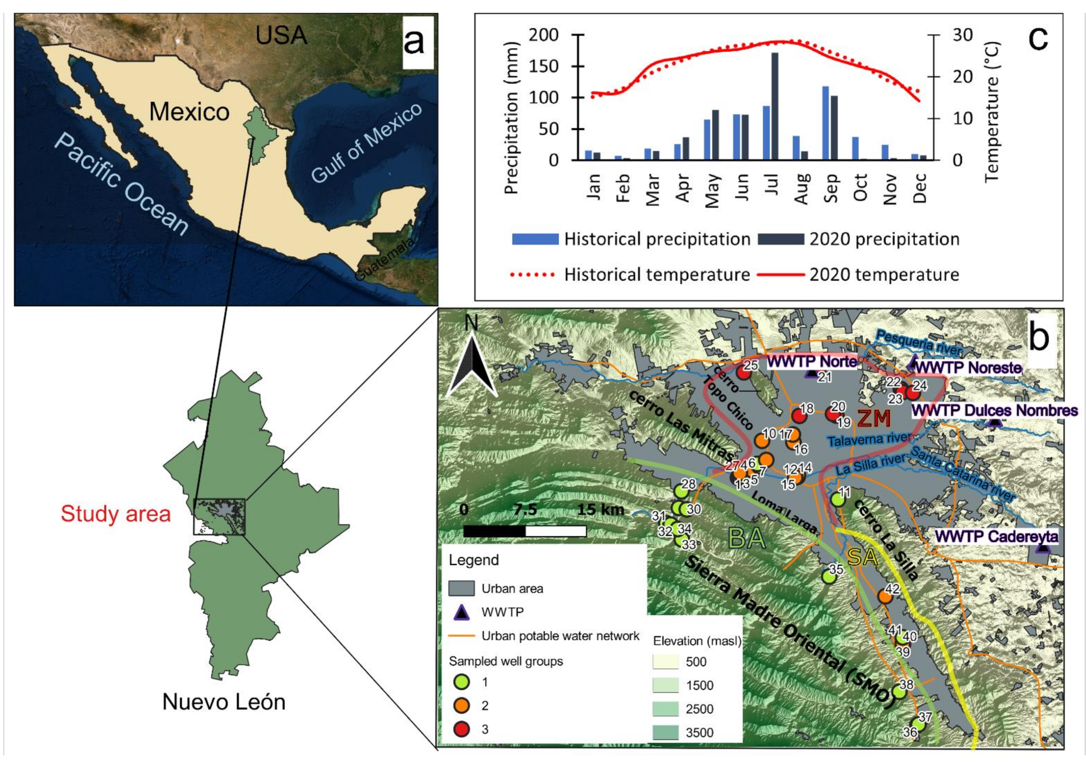
2.1. Study Area

Monterrey is the second largest city in Mexico, according to population and economic growth. It consists of twelve municipalities hosting about 5.3 million inhabitants [27]. It represents an important business and industrial center covering approximately 6680 km2, accommodating many national and international industrial companies and technological enterprises.
The MMA is located around the foothills (north–northeast) of the Sierra Madre Oriental (SMO) cordilleran belt shaped by several mountains arising from the west (Cerro Las Mitras) to the southeast (Cerro La Silla), and hills from the northwest (Cerro Topo Chico) to the south (Loma Larga), with elevations ranging from 450 to 3500 metres above sea level (m.a.s.l.) (Figure 1). Clastic marine to carbonate sedimentary rocks have been identified within the cordillera (SMO) that limits the MMA to the west and south of the region. Toward the north to the northeast, the MMA lies in a valley filled with Quaternary alluvial detritus mainly composed of fluvial and alluvial sedimentary deposits as a result of erosion–accumulation cycles since the early Quaternary period [28]. Most of these recent deposits can be found as riverbeds in the La Silla and Santa Catarina Rivers, which flow eastward towards the Gulf Coastal Plain. Sediments from the alluvial deposits include uncemented small cobble to pebble gravel, gravel sand, sand, and silts cemented by calcite [29].
The climate around the MMA is semi-arid, with a mean annual rainfall and temperature of 622 mm and 22.7 °C, respectively, characterized by a rainy and a dry season. Typically, the rainy season spans from May to October, while the dry season lasts from November to April. Figure 1 shows the precipitation and temperature comparison between historical trends (1951–2021) and the 2020 trend in the MMA. From a historical perspective, May, June, and July have similar precipitation values, reaching mean monthly values of up to 75 mm. August is characterized as being the driest month within the rainy season by accumulating, on average, less than 40 mm of precipitation. However, September tends to be the rainiest month of the season, accumulating about 120 mm of rainfall. Nevertheless, every 3–4 years, heavy rain events add 100 mm or more within 24 h periods, often associated with tropical storms and/or hurricanes [30]. Therefore, it is no surprise that local rivers and creeks carry minimal flows all year round.
Accordingly, the year 2020 was the second consecutive year with precipitation values below historical averages (<622 mm), ending with a 5-year rainfall deficit in the 2010–2020 decade [31]. Heavy rainfalls from the tropical storm “Hanna” on July 2020 caused overflows along MMA streams and creeks, triggering several landslides from subsoil water saturation and interrupting traffic access in some areas from river overflooding [31]. Interestingly, the months of August and October showed precipitation values that were 95% and 64% lower than the mean monthly precipitation recorded historically, respectively.
The water supply for the MMA region is apportioned by surface water (volume 58%) and groundwater (42%) reservoirs [32]. The proportion might vary from year to year. Groundwater is retrieved from several aquifer units and wellfields, which are treated locally for consumption before being transferred into the city’s drinking water supply network [33]. The aquifer units governing the MMA groundwater and considered in this study are (1) the Buenos Aires (BA) wellfield, (2) the Santiago system (SA), and (3) the Zona Metropolitana de Monterrey (ZM) aquifer. The BA wellfield (2.11 m3/s) consists of 23 deep wells (water table depth below ground: 20–120 m) from Early Cretaceous limestone formations mainly dominating the SMO. The SA system (1.27 m3/s) comprises 3 infiltrating galleries from the southern sections of the La Huasteca mountain front and several shallow wells (water table depth below ground: 20–50 m) along the Santiago Valley. Lastly, the ZM aquifer (1.08 m3/s) incorporates scattered wells throughout the metropolitan area from a shallow (3–20 m water table depth) aquifer consisting of Tertiary gravel, sand, and clay detritus along conglomerates (Reynosa Formation) and altered lutites (Mendoza Formation) [34]. Further details on the hydrogeological and hydrogeochemical conditions of the study area can be found in previous studies of the MMA [33,35].

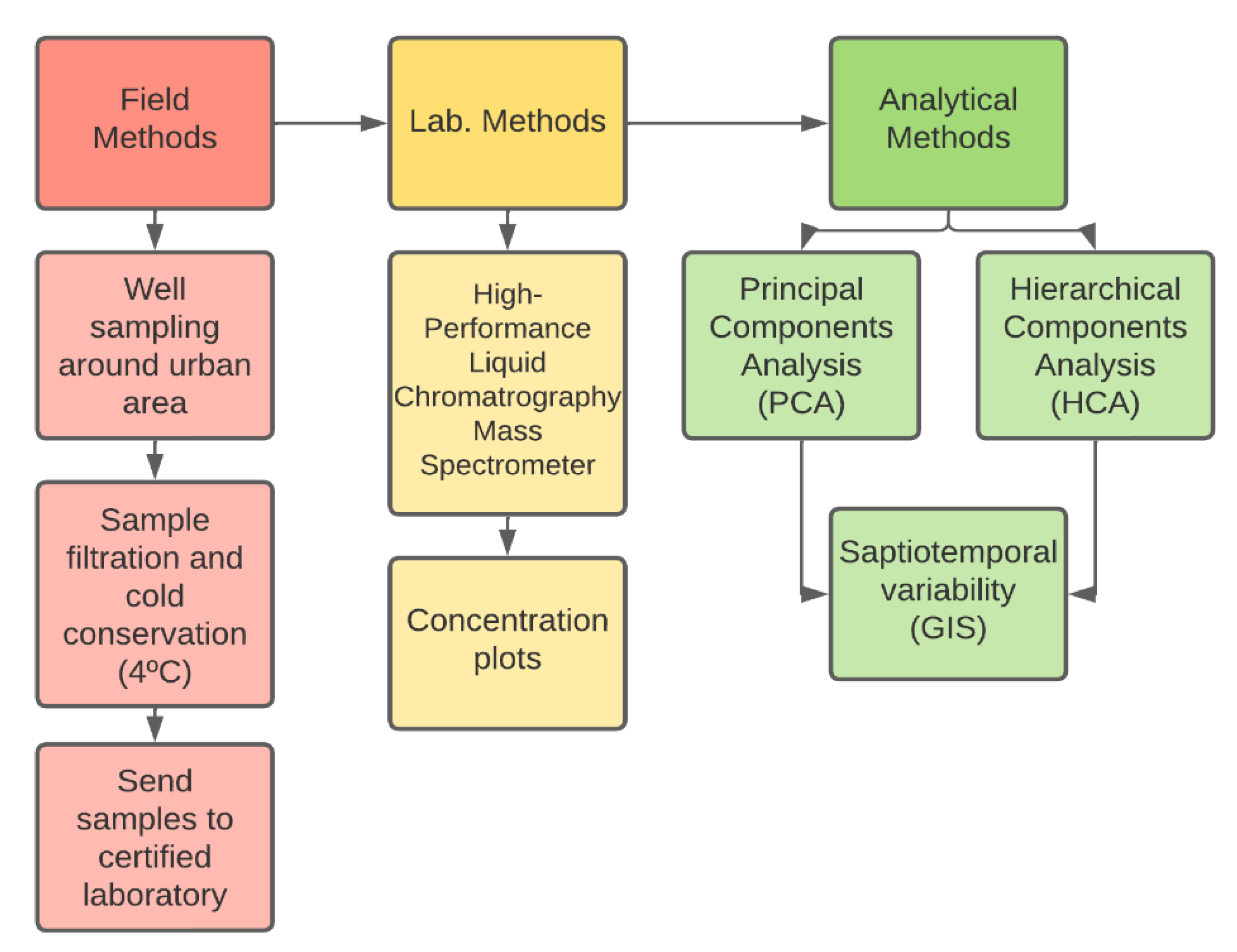
2.2. Field and Laboratory Work

Two sampling campaigns were carried out in 2020, considering water supply wells for the MMA. Five wells located in the ZM aquifer were initially monitored from 15th to 16th March 2020, as an approach for surveying Asws occurrence in the area. The second field campaign considered samples from 42 sites from the ZM (27) (including the previous 5 from initial field campaign), BA (8), and SA (7) aquifer units and took place from October 29th to November 6th, 2020 (Figure 1c). The five wells from the first campaign were resampled. A summary of the applied methods is shown in a schematic flow diagram (Figure 2). All surveyed wells form part of the well network of the Monterrey’s water and sanitation utility and are equipped with pre-installed pumps and hydraulic equipment pertinent to the operation. Field parameters, i.e., pH, temperature, electrical conductivity (EC), oxidation–reduction potential (ORP), dissolved oxygen (DO), and total dissolved solids (TDSs), were measured on-site using pre-calibrated electrodes (YSI® Professional Plus, OH, USA). Samples were collected in sterile pre-rinsed polyethylene bottles and then stored in an icebox until filtration. All water samples were filtered through 0.45 µm pore-size cellulose nitrate membrane filters using a vacuum medium and placed in HDPE bottles on the same sampling day. Alkalinity was measured via the titration method using HCl 0.1 M as the titrant until a pH value of 4.3 was reached. Samples for cation analysis were stored after filtration in 250 mL HDPE bottles and preserved with ultra-pure HNO3 at pH < 2 to avoid element precipitation/adsorption during storage. Samples for anion analysis and artificial sweeteners were placed and stored in HDPE bottles with capacities of 250 and 125 mL, respectively.
The concentrations of major ions (Ca2+, K+, Mg2+, and Na+) and dissolved B and Si were measured by ICP-OES using a Perking Elmer Optima 2100DV instrument. Meanwhile, anion concentrations (Cl, SO42−, F, NO3, NO2, Br, I, and PO43−) were determined using a Dionex DX-120 ion chromatograph, Thermo Fisher Scientific, Waltham, MA, USA. To maintain data quality after completion of analytical procedures, the charge balance error (CBE) was calculated using the following equation:
CBE = c a t i o n s m e q L a n i o n s   m e q L c a t i o n s m e q L + a n i o n s   m e q L         ×         100
In this study, the mean value of CBE was equal to 1.8%, with 95% of the samples being in the interval [0–±5%] and the remaining 5% in the interval [0–±9%], which indicated that the results analysis was considered reasonable.
Regarding the analysis of Asws, the solid-phase extraction (SPE) method was used to isolate analytes and remove any interfering compounds from the groundwater samples. Strata X cartridges (200 mg/6 mL; Phenomenex, Aschaffenburg, Germany) were used to perform the analysis. A vacuum manifold setup from IST was used for SPE. Preceding the SPE method, the groundwater sample pH was adjusted with hydrochloric acid. Cartridges were conditioned with 3 × 3 mL of methanol followed by 3 × 3 of ultra-pure water to set the pH of each sample. Subsequently, water samples were passed through the cartridges, and the loaded sorbent materials were dried using a subtle nitrogen stream. Analytes were eluted with 3 × 3 mL of methanol if the anion or cation exchange capacity of the sorbent was null. Strong cation exchange material (MCX) and weak anion exchange material (WAX) were eluted with methanol (80:20, v/v). SPE extracts were evaporated to dryness with a nitrogen stream and reconstituted with 400 µL of solvent A and 100 µL of solvent B used for liquid chromatography.
Artificial sweeteners (ACE, SUC, CYC, SAC, and ASP) were analyzed at Technologiezentrum Wasser (Karlsruhe, Germany) in accordance with the German standard method DIN 38,407 part 47 [36]. High-performance liquid chromatography was carried out using an HPLC 1290 (Agilent Technologies, Santa Clara, CA, USA) model equipped with a quaternary pump, a thermostated column compartment, a micro vacuum degasser, and a standard autosampler. The setup was coupled to a Triple Quad 5500 (ABSciex, Framingham, MA, USA) mass spectrometric detector (MS/MS) with an electrospray (ESI) interface.
Chromatographic retention and separation were accomplished using a Zorbax XDB-C8 column (150 × 2.1 mm; 3.5 µ) from Agilent Technologies. A gradient consisting of (A) 10 mM ammonium acetate in water and (B) 10 mM in methanol was used for separation. The gradient sequence began with 90% of eluent A, which was decreased to 25% A in 6 min, kept isocratic for 5 min, and then returned to initial conditions within 1 min. The column was re-equilibrated after 9 min before each injection. Separation occurred at 40 °C with a flow rate of 0.30 mL/min. Such a flow was chosen for optimum chromatographic performance during the methodological process, and thus was kept constant thereafter. The injection volume was 15 µL. To reduce the carryover risk from the injector port, the injector needles were automatically washed with methanol after each injection.

2.3. Statistical Analysis and Interpretation Techniques

Multivariate statistics is a common approach applied to give insights into groundwater classification and to explore relationships between a set of hydrochemical parameters. This study performed hierarchical cluster analysis (HCA) using SPSS 26.0 [37]. The aim of HCA is to classify samples into two or more groups based on the resemblance of such samples due to special characteristics. Field parameters (temperature, pH, electrical conductivity, dissolved oxygen, and ORP), major cations (Ca2+, Mg2+, Na+, and K+), anions (HCO3, F, NO3, Cl, SO4, Br, I, and PO4), B, dissolved Si, and artificial sweeteners (ACE, ASP, CYC, SAC, and SUC) were evaluated through HCA. To arrange the graphical plots and simplify the statistical analyses, values below detection limits (DLs) were reported as 0.5 of the DL values. Generally, most chemical parameters do not follow a normal distribution amongst datasets. Therefore, a compositional data method known as centered log-ratio (clr) transformation was applied to avoid pseudo-correlations and reduce the consequence of data outliers for HCA analysis by achieving a more symmetrical distribution of the data [33,38]. The clr transformation was conducted by dividing each component (x) by the geometric mean g(x) of all variables in accordance with Equation (2):
clr x i = l n x i g x
To classify groundwater sampling groups during the HCA, the Euclidean distance and Ward’s method after data transformation were applied. Each resulting group normality was analyzed with the Shapiro–Wilk test (p < 0.05) for the groundwater sampling population below fifty (n < 50) (Table S2, Supplementary Materials), while variable differences within groups were compared using an analysis of variance (ANOVA) test at a p < 0.05 significance level. The Spearman rank correlation was applied under the assumption that the resulting groups had a monotonic relationship between the hydrogeochemical parameters and the Asws concentrations.

3. Results

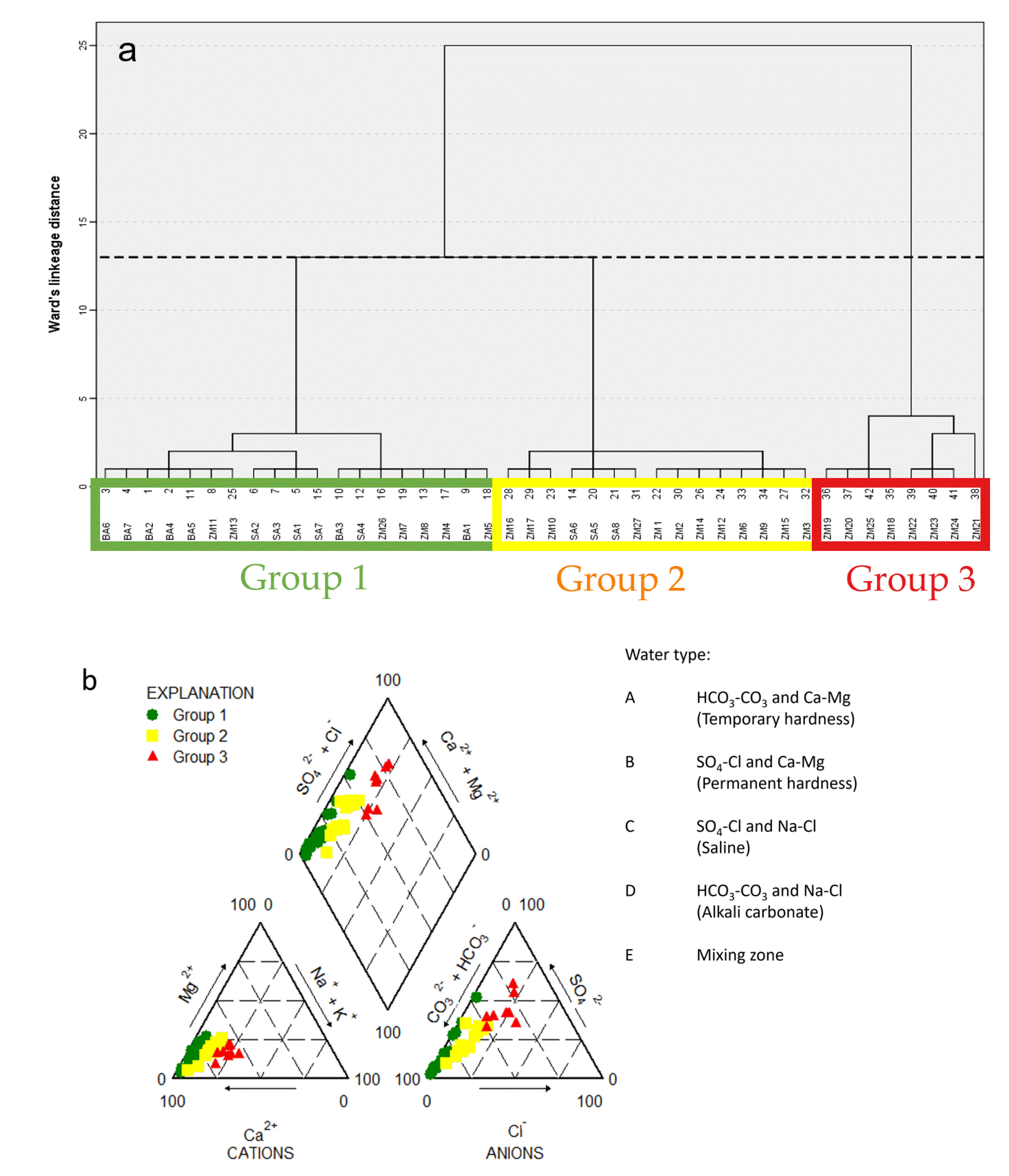
3.1. Groundwater Sampling Groups and Hydrochemical Description

A summary of the descriptive statistics for the physicochemical parameters, major ions, and artificial sweeteners is shown in Table 1. Group results after HCA are depicted in Figure 3a using a dendrogram. Three groups of water samples were defined by the chemical similarities of samples from the horizontal phenom line below 13 using the Ward method linkage distance algorithm. Group 1 indicates samples in the recharge zone along the SMO mountainous area. Group 2 clusters wells in the transition zone along the southern area of the MMA valley. There are no WWTPs near group 1 and 2 areas (Figure 1). In contrast, group 3 is quite different from the first two groups. This last group highlights NO3-polluted water samples from groundwater discharge areas mainly along the northernmost part of the MMA [32] (Figure 1c). Most parameter average values suggest water quality degradation with the increasing groundwater flow path. There are two existing and operating WWTP along the northern area of the MMA (near wells 21–25), where leaks from the sewage network are presumably existent. Most parameter values increased from the first to the third group, indicating degradation of the water quality.
In all three groups, the temperature fluctuated between 17.3 and 30.9 °C, the redox potential varied from 208 to 572 mV, and DO ranged between 1.5 and 6.5 mg/L. However, no significant differences were found in these parameters across the three groups. Regarding pH, groundwater samples from groups 2 and 3 showed mean neutral values (7.4–7.7), whereas group 1 samples were more likely to have higher alkaline values (8.3 ± 0.5), which were significantly different from those of the previous groups (p < 0.05). Mean EC and TDS values exhibited significant differences (p < 0.005) in all three groups. For group 1, EC and TDS mean values were 424.8 µS/cm and 279.4 mg/L, respectively. Groups 2 and 3 had mean EC and TDS values of 760.1 µS/cm and 496.6 mg/L, and 1410.9 µS/cm and 913 mg/L, respectively.
Similarly, the mean values of major ions such as Cl, NO2, NO3, PO4, and Na+ for groups 2 and 3 were significantly higher than those of group 1 (p < 0.05). The concentrations increased in the order of group 1 (Cl: 8.9 mg/L; NO2: 0.01 mg/L; NO3: 2.3 mg/L; PO4: 0.02 mg/L; and Na+ 5.5 mg/L) < group 2 (Cl: 37.9 mg/L; NO2: 0.02 mg/L; NO3: 9.9 mg/L; PO4: 0.04 mg/L; and Na+ 19.7 mg/L) < group 3 (Cl: 118.9 mg/L; NO2: 0.05 mg/L; NO3: 20.2 mg/L; PO4: 0.01 mg/L; and Na+ 64.8 mg/L). Moreover, B and Br were also found to have significant differences between groups (p < 0.05), where concentrations increased in the order of group 1 (B: 20.1 µg/L; Br: 27.7 µg/L) < group 2 (B: 75.3 µg/L; Br: 121 µg/L) < group 3 (B: 179.8 µg/L; Br: 309.3 µg/L). In addition, the concentrations of the major ions Ca2+, Mg2+, K+, HCO3, F, and SO42− in groups 2 and 3 were significantly higher (p < 0.05) than of those of group 1.
A trilinear diagram was developed for the MMA groundwater using the analytical data acquired from groundwater collected in the sampled wells (Figure 3b). The three groundwater groups defined by the HCA are confined to a Ca–Mg and HCO3–CO3 type, a Ca–Mg and SO4–Cl type, and a mixing zone type. Groundwater samples from the Buenos Aires wellfield and the foothills of the SMO (group 1) had significantly lower concentrations of major ions (Ca2+, Mg2+, K+, Na+, HCO3, Cl, NO3, SO42−, PO43−, and Si), EC, and TDS than groups 2 and 3, resembling a Ca–HCO3 water type, i.e., this group represents the least mineralized waters within the studied area because these samples were taken in recharge zones (Figure 2c and Figure 3b). Due to their topographic features, waters from this group may have a shorter groundwater flow path interacting with weathered carbonates from the SMO. This compositional trend is deemed consistent with previous reports [33].
In contrast, the groundwater samples clustered in group 2 showed a slight shift towards a more mixed water type, whereas most samples remained within the type-A area (trilinear diagram). Samples from group 2 were located within the MMA limits inside the valley of Monterrey, having significantly higher concentrations of major ions (K+, Na+, HCO3, Cl, NO3, and PO43−) Si, EC, and TDS than group 1, indicating a water source mixing influence. These waters have strong interactions with carbonate, silicate, and evaporite rocks as they flow from the SMO and transit the alluvial sediments and calcareous shales of the Mendez Formation within the Monterrey Valley [35] (Figure 1c and Figure 3a). Waters from group 2 (Figure 3b) showed a shifting transition to a Ca-HCO3-SO4 water type, which classifies this area as a transition zone. Consequently, nitrate concentrations were significantly different (p < 0.05) and greater than those of group 1, indicating the existence of NO3 sources from an anthropogenic influence in this water group [33].
Lastly, waters from group 3 fell within the mixing zone and Ca-SO4 water types (Figure 1b and Figure 3b), resembling the most mineralized group. Wells from this group are located at the northernmost point of the MMA in the direction of the groundwater flow (SW to NE). This group had significantly higher concentrations of HCO3, Cl, NO3, SO42−, Ca2+, Mg2+, Na+, B, Br, and I than the other groups. A closer inspection of waters in group 3 revealed that NO3 concentrations were above the Mexican drinking water standard (10 mg/L for NO3-N) (Table 1), and thus above the threshold value of 3 mg/L for anthropogenic influence [41].

3.2. Concentration of Asws in Groundwater

Concentrations of Asws were measured in wells 3, 6, 9, 14, and 16 (n = 5) in May and later in November of 2020. These five wells were clustered into group 2 after HCA. ACE and SUC were present in significant amounts (p < 0.05) in both sampling campaigns, whereas concentrations of CYC and SAC decreased between May and November. ASP was below detectable limits (BDLs) in all wells from both sampling campaigns. During May, average ACE and SUC concentrations were 0.038 µg/L and 0.35 µg/L, respectively. Average concentrations for ACE and SUC in the November campaign were 0.03 µg/L and 1.2 µg/L, respectively. Notably, while ACE concentrations exhibited no significant decrease (May, 0.19 µg/L and November, 0.11 µg/L), showing no significant temporal variation between datasets, SUC concentrations increased more than threefold (May, 0.35 µg/L and November 1.2 µg/L) between temporal datasets. SUC concentration increments between datasets confirm: (1) continuous input of this sweetener in those areas from anthropogenic activities; (2) SUC is recalcitrant with very low degradation rates; and (3) it is proof that urban wastewater is percolating into the shallow aquifer. It is important to note that no WWTP was found near these sampling sites, which led to the inference that pipeline leakages are likely to occur before sewage reaches the city’s WWTPs.
Concentrations of Asws in the November 2020 groundwater samples (n = 42) from the MMA are presented in Figure 4. ACE and SUC were the two most abundant out of the five Asws measured in the MMA. ACE was found in 57% (24 out of 42) of the sampled wells, while SUC had an occurrence of 55% (23 out of 42). In contrast, SAC was detected in fewer than 15% (5 out of 42) of samples from the study area, whereas the remaining samples had concentrations below the quantification limits (BQLs). Conversely, ASP and CYC were not found (BQL) in water samples in all three groups. Mean concentrations of ACE and SAC showed an increasing trend in the order of group 1 (ACE: 0.01 µg/L ± 0.008; SAC: 0.005 µg/L ± 0.002; SUC: 0.05 µg/L ± 0.09) < group 2 (ACE: 0.03 µg/L ± 0.01; SAC: 0.006 µg/L ± 0.003; SUC: 0.92 µg/L ± 0.8) < group 3 (ACE: 0.45 µg/L ± 0.01; SAC: 0.008 µg/L ± 0.007; SUC: 0.67 µg/L ± 0.5), which is consistent with the increasing trend shown by NO3 in each area: recharge area < transition zone < discharge area. This trend has also been observed in other urban environments worldwide [4,6,8,16]. However, when evaluating SUC occurrence, the mean value was significantly higher in group 2 (p < 0.05) than in groups 1 and 3.
Several factors may determine the amount of Asws in MMA groundwater. Primarily, pollution and chemical mixing occur in the upper soils mostly composed of alluvium with high porosity and permeability rates [33]. Therefore, such soils could be contaminated by sewage spills in the most urbanized areas (groups 2 and 3). Some of these Asws are added to a wide variety of processed products of daily consumption amongst the local population, entering the soil through an inadequate sewage system, especially in the downtown area. The solubility and persistence of the target Asws are key factors influencing the chemical transfer from the upper soil layers after spills into the urban aquifer. A remarkable observation is that the highest concentrations of total Asws were found in four and two wells of groups 2 and 3, respectively. Total Asws concentrations of 2.9, 2.7, 1.8, 1.2, and 1.0 µg/L were recorded in wells 42, 6, 2, 9, and 16, respectively, which belong to group 2. It should be noted that these wells are in areas of commercial activity within densely populated sections of the MMA and near the main urban Santa Catarina River. Similarly, total Asws concentrations of 1.4, 1.3, and 1.0 µg/L were measured in wells 19, 20, and 24, respectively, clustered in group 3. The first two wells are in a densely populated urban area with several local bakeries operating in the area continuously, and the third well is located within an industrial area where soft drinks and other commercial beverages are produced. Elevated ACE or SUC concentrations may be attributed to a recent source of contamination, most likely wastewater or septic plumes in shallow aquifers [16,42,43]. These factors explain how the occurrence of Asws in the MMA is attributed to diffuse sources. However, the existence of these and other non-point pollution sources, such as commercial producers using Asws around the well areas, leakage from the municipal sewage network, and/or surface runoffs is hard to identify.

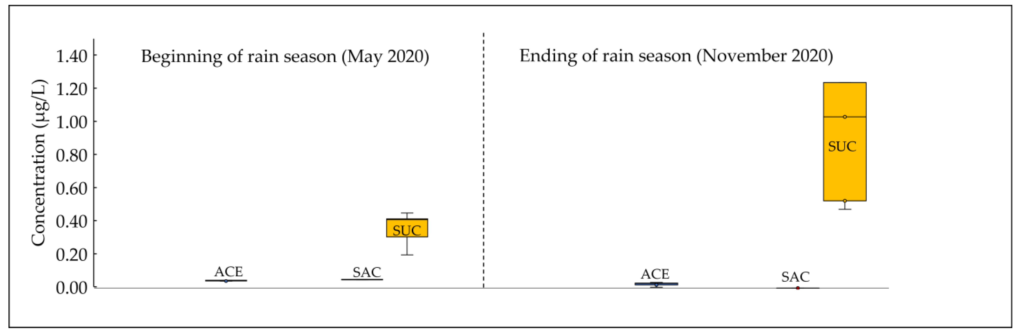
3.3. Temporal Variation in Asws Concentrations

The seasonal variation in concentrations of Asws in the groundwater samples of group 2 is shown in Figure 5. To assess the Asws changes over time, the Kruskal–Wallis test was applied between the samples collected in May 2020 (beginning of the wet season) and samples collected in November 2020 (end of the wet season). Five samples from the transitional water group (group 2) were compared between the two temporal datasets. The test evaluated whether Asws concentrations have significant differences (p < 0.05) between climatic seasons (Table S3, Supplementary Materials). The results show that dominant Asws concentrations at the start of the rainy season (May 2020) were in the order of SUC (mean of 1.18 µg/L) > ACE (mean of 0.19 µg/L). However, at the end of the wet season (November 2020), mean concentration values for ACE slightly decreased (0.11 µg/L; no significant temporal differences were found), whereas SUC mean concentrations were significantly higher (p < 0.05) than those retrieved at the beginning of the wet season. As described above, the year 2020 is considered a rather dry year because the mean monthly precipitation was reported to be below the historical average. However, soil saturation during July from the intense rain events caused by tropical storm Hanna may have been an important contribution to the mobility of Asws along the MMA aquifer (Figure 1). This trend could be confirmed through a monitoring scheme of the MMA wells over time. However, a possible interpretation of these increases in concentrations is that four out of five of the sampled wells are near hospital facilities, malls, and industrial manufacturers located at lower gradients near the Santa Catarina River, which are areas that typically receive wastewater discharge carrying oil residues, soaps and detergents, paints, and septic waste [44]. The remaining well is in a transited urban area with small business and commercial activities. Inherent to the location, another possible interpretation for the Asws concentration variation could be the occurrence of the coldest periods. The warmer ambient temperatures recorded during May 2020 (26.6 °C) in comparison with the lower temperature values during November (Figure 1) might play a key role in degrading SUC in aqueous media at the beginning of the rainy season [45]. Correspondingly, the mobilization of SUC from the unsaturated zone to the aquifer due to high rainfall rates and colder temperatures (in the order of 15 °C) at the end of the rainy season may concentrate SUC in the groundwater, leading to higher SUC concentrations.

4. Discussion

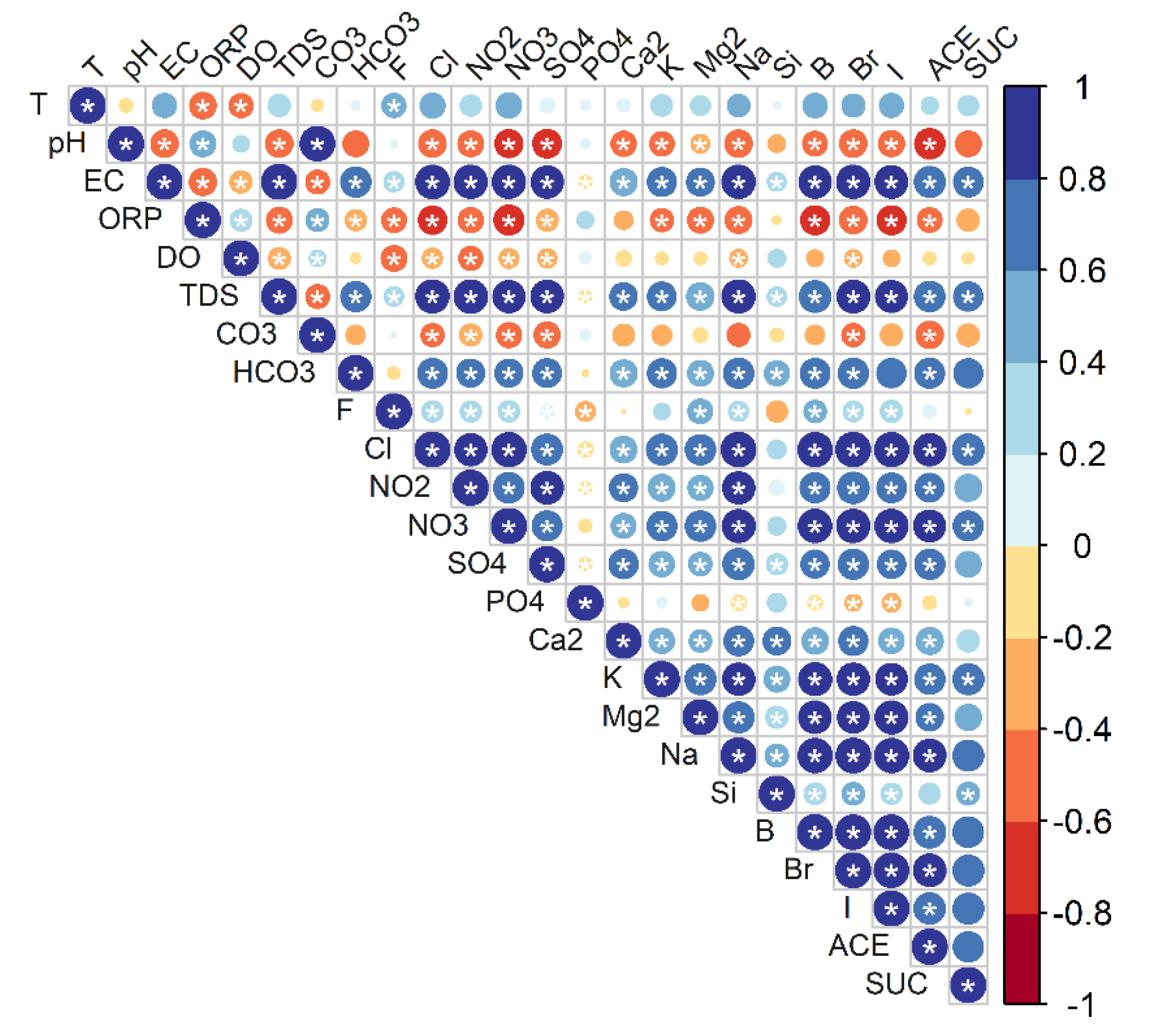
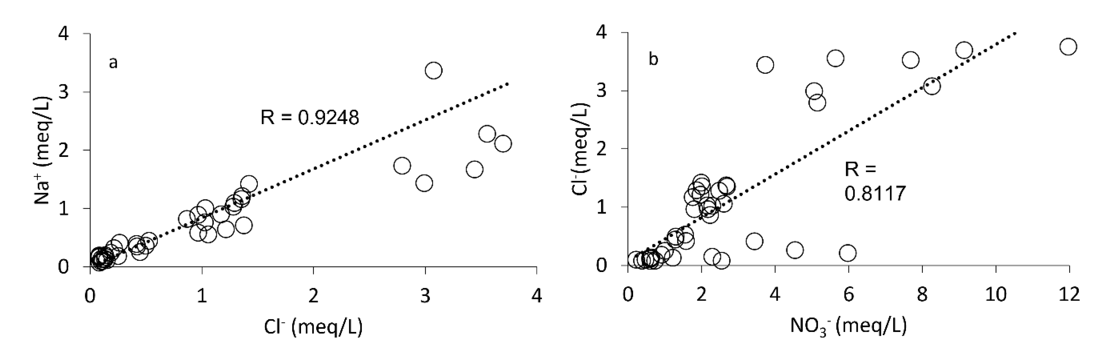
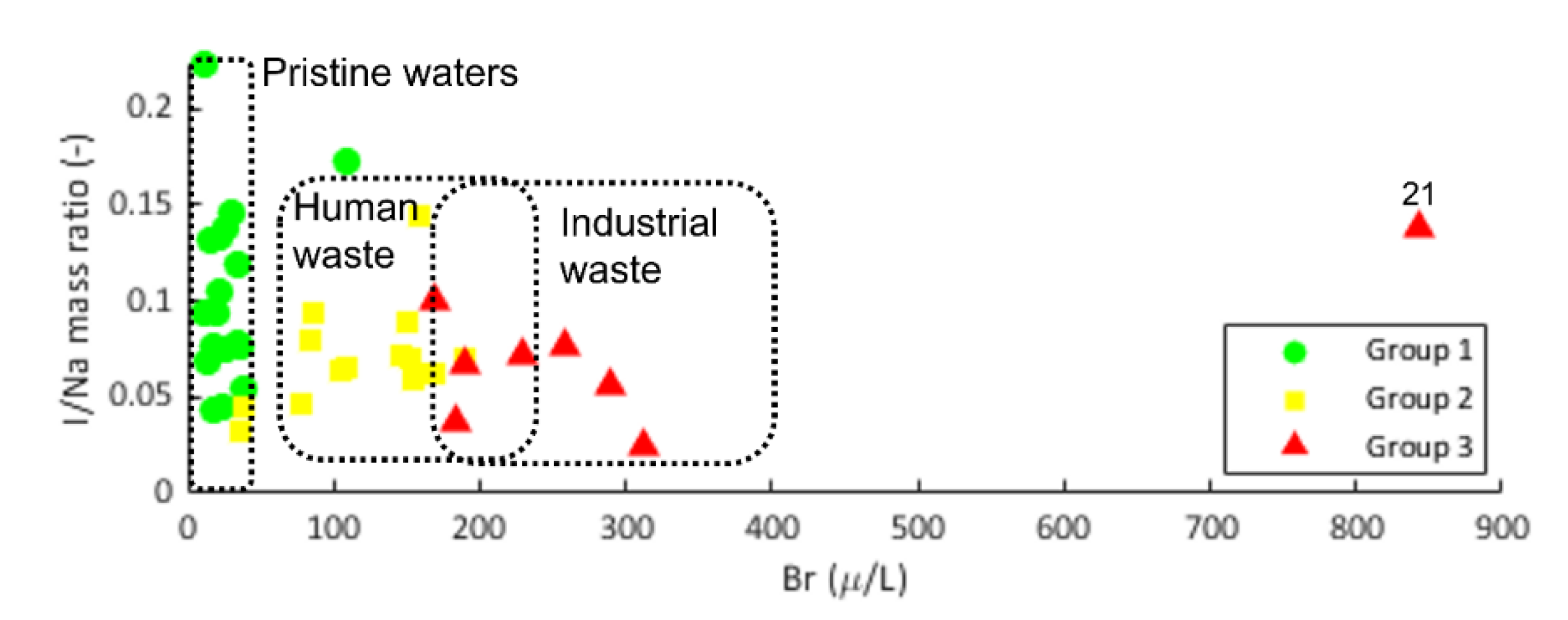
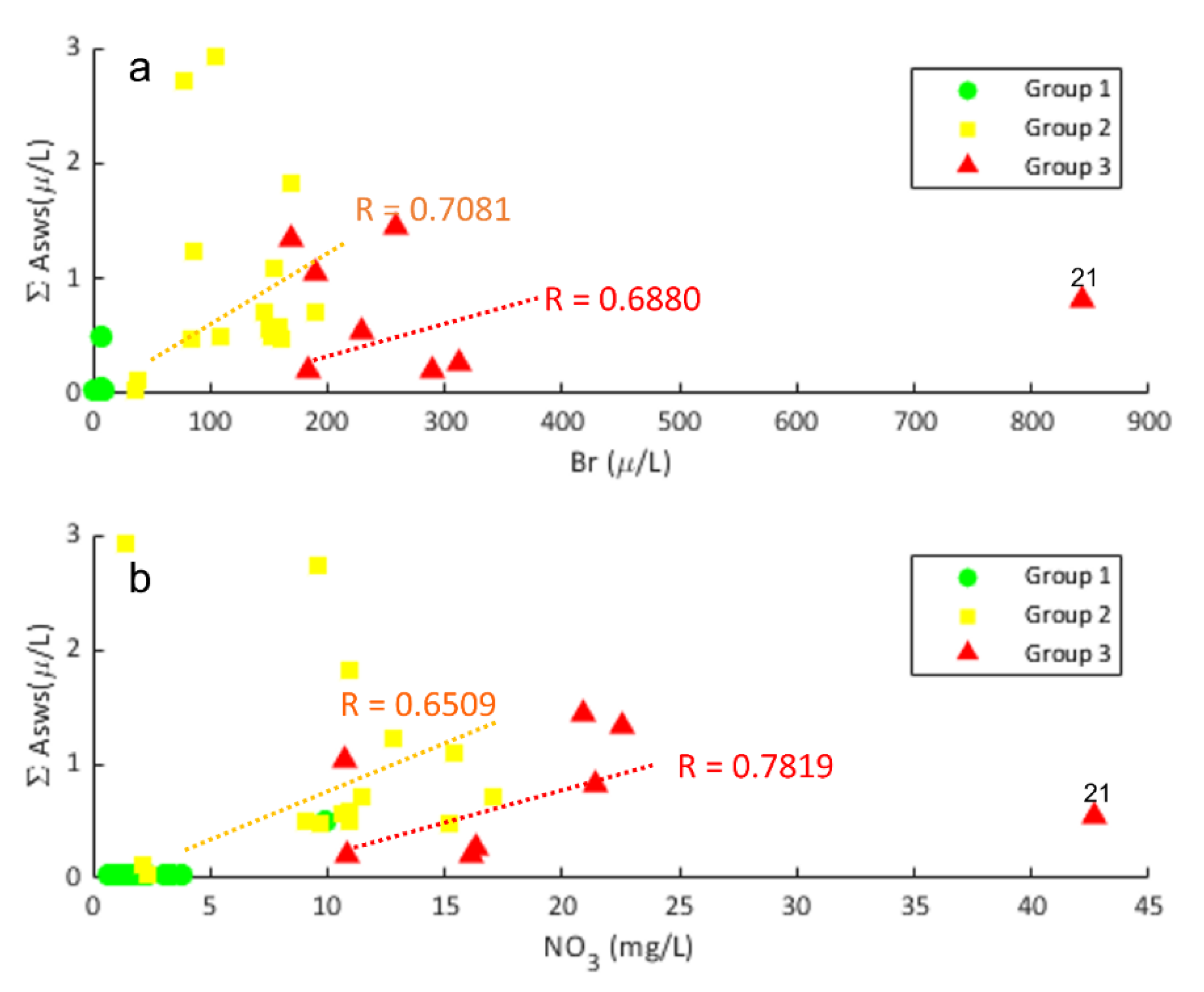
4.1. Association of Asws with Hydrochemistry

Processes that regulate groundwater compositions and solute origins can be determined from compositional relationships between the dissolved compounds [46]. Each parameter was checked for normality using the Shapiro–Wilk test (Table S2, Supplementary Materials). In all cases except for temperature, values of this test were equal to or less than 0.05, which indicates that all measured groundwater parameters except temperature were non-normally distributed. As a result, the non-parametric Spearman rank correlation method was employed to measure correlations between variables (Figure 6). Consequently, EC correlated with TDS, having Na+, Cl, and SO42− as the main constituents. Similarly, NO3, I, B, Br, HCO3, K+, Ca2+, Mg2+, ACE, and SUC were highly correlated with TDS. It is evident that groundwater salinity is supplied by these major elements.
The significant positive correlation between Ca2+ and Mg2+ and EC relates these two parameters as water hardness factors. Similarly, the stronger positive correlations between Cl, Na+, Br, NO3, I, B, SO42−, HCO3, ACE, and SUC and EC indicate that these compounds in groundwater increase together with the flow path. The strong positive correlation between Cl and Na+ ions (r = 0.95) shows that the groundwater has a strong interaction with salt rocks such as halite. Nonetheless, it is known that Cl and Na+ can also come from anthropogenic sources, mostly agricultural fertilizers, animal waste, and septic sewage from domestic and industrial activities [47]. It has been proven that Na+ released from silicate weathering is mostly confirmed with a Na+/Cl molar ratio greater than 1 [48,49]. Therefore, a Na+/Cl ratio with approximate values near 1 generally interprets halite dissolution as a major process. In contrast, lower average values (<0.7) can be interpreted as a wastewater influence. As shown in Figure 7a, the molar ratio of Na+/Cl fell below the equiline, with depleted Na+ and elevated Cl, revealing that other Cl sources aside from halide dissolution occur in the MMA. Furthermore, the moderate positive correlation (r = 0.65) between Cl and NO3 (Figure 7b) indicates that the resulting Cl ions come from an anthropogenic influence. In this study, Cl enrichment might have occurred due to sewage infiltration, since groups 2 and 3 exhibited mixed water types typical of urbanized discharge areas [33]. A variety of methods have been used to assess possible sources of Cl and Na+ in polluted groundwater. One of these is plotting halide (I, Cl, and Br) ratios as proxies for tracing wastewater pollution [33,41,50]. Generally, halides do not change in natural conditions, having minimal interactions with substrates as they migrate through the groundwater. Hence, mixing diagrams have been developed considering different sources of contamination such as treated sewage effluents, septic tank leachates, diluted groundwater, and urine [50,51].
Figure 8 illustrates three classifications based on the I/Na mass ratio vs. Br, indicating pristine waters (group 1), urban-affected water (group 2), and a mixture of water affected by urban wastewater and wastewater derived from the food industry (group 3). High concentrations of I have been identified in contaminated shallow groundwater derived from landfill leachates, medical products, and animal additives [41,50]; therefore, the plot of I/Na ratios vs. Br concentrations is useful for elucidating contamination sources in groundwater resources. Increases in Br concentrations can be observed between groups, creating an overlay between groups 2 and 3. Overall, although the groundwater of group 2 strongly interacts with carbonates, silicates, and evaporitic rocks, it has a wastewater influence as it flows through a heavily populated business district in the urban area [33,35]. Similarly, the groundwater of group 3 falls in the range of water strongly affected by urban and industrial wastewater, which seems consistent with the well locations in the northwestern MMA, where there is an important industrial sector.
For all groundwater samples taken on November 2020, strong positive correlations were observed between Br and NO3-N and ACE (r = 0.85 and r = 0.81, respectively; p < 0.001) and SUC (r = 0.77 and r = 0.71, respectively; p < 0.001) (Figure 6). This suggests that elevated concentrations of nitrates measured in wells located in the MMA shallow aquifer (groups 2 and 3) were derived from the wastewater infiltration into the aquifer system, which has been previously reported using a Bayesian isotope mixing model [33]. This confirms the suitability of Asws as markers of sewage leakage pollution in groundwater, because these compounds can be found as high-production-volume chemicals characterized by their high persistence in the environment and recalcitrant behavior in groundwater [2,4,5,13].
As illustrated in Figure 9a,b, specific samples from groups 2 and 3 showed a positive correlation between total Asws and B and NO3. This may indicate a sewage impact from restaurants and coffee shops located in the city center, because Asws are low-calorie sugar substitutes widely used in a variety of foods as additives, soft drinks, sanitary products, and pharmaceutical compounds of daily usage [2,4]. While most groundwater samples showed consistent enrichments of Br and NO3 with Asws, an outlier of sample 21 (group 3) revealed maximum concentrations of Br, indicating that other sources of pollution also impact the aquifer in this area. Production well 21 is in northern Monterrey, near the Pesquería River and a wastewater treatment plant (WWTP Norte) that receives wastewater from this area. Therefore, greater contamination is expected in this area because the Pesquería River receives wastewater effluents from the nearby WWTP. Indeed, due to the overextraction of groundwater in that zone, the Pesquería River waters may infiltrate into the aquifer, increasing pollution in the groundwater.
One unanticipated finding was that the higher Asws concentrations were measured in wells clustered in group 2 (Figure 8), although we expected that total concentrations would be higher in the discharge area (group 3). One possible explanation for this outcome is that wells in group 2 are continuously polluted from possible sewage leaks from businesses that offer Asws to consumers along the MMA downtown area (where higher Asws concentrations are recorded), while periods of heavy rains aid in washing-out these compounds as they naturally flow in the north–northeast direction exiting the MMA’s urban/industrial limits, making Asws concentrations lower than previous group. Previous studies reported that similar pollution sources imply strong correlations between co-tracers [13]. In contrast, different pollution sources might reveal differences in their relative concentrations, thus weakening the correlation between co-tracers. This relationship can, in part, be explained by the differences in the sum of Asws per analyzed group. The concentrations of Asws, supported by other parameters (Br and NO3), clearly show that the shallow groundwater samples from group 2 were influenced by modern wastewater sources. Total ACE (0.49 µg/L) was found at much lower concentrations than total SUC (13.82 µg/L) in group 2. Therefore, different pollution sources are pathways for both Asws into the MMA shallow aquifer.
A social study on Asws consumption in Mexico reported that at least 96% of the population (n = 150) consumed a product with Asws daily in Mexico without “knowing” that such a product had any of the studied sweetening components [52]. This study also classified the percentage of Asws (ACE 90%; ACE+ASP 86%; SUC 80%; and SUC+ACE 39%) available in most consumed products (sugar substitutes 66.7%; soft drinks 60%; gelatins 48.7%; chewing gum and breath pills 46%; yogurts 36%; marmalades 19.3%; cookies 12%; and desserts 5.3%) on a daily basis [52]. The geographical location delineated by wells in group 2 is mainly occupied by business centers (mostly office headquarters of major local companies). The area also hosts food courts, bakeries, and coffee shops. Consequently, infiltration from food courts/bakeries/coffee shops may influence the presence and occurrence of Asws in the area. If the previous assumption is true, then the occurrence of Asws entering the shallow urban aquifer is through leaky sewers and surface runoffs in the surrounding location. A similar trend was observed for ACE (0.36 µg/L) and SUC (5.38 µg/L) concentrations in group 3, which may support the previous statement.
According to the National Statistics of Economic Units Directory (DENUE), which represents an interactive platform where the Mexican government registers commercial activities throughout the national territory, the MMA hosts about 54,553 businesses operating continuously through a variety of services in the surroundings of wells from group 2 [53]. Therefore, large amounts of wastewater are produced in the area, carrying large amounts of Asws, of which a fraction ends up percolating in the shallow aquifer and mixing with the groundwater. However, the major fraction of wastewater is transported to the WWTP through the municipal sewage network.
A second interpretation regarding the decreasing concentrations of Asws between groups 2 and 3 within the same sampling period is that SUC (the most abundant Asws in the groundwater of groups 2 and 3) underwent biodegradation processes with the septic sludge within the drainage network. Other studies reported that a slow reduction in SUC concentrations is consistent with the slow and incomplete mineralization of SUC in sewage under aerobic conditions [5]. Thus, decreasing concentrations of SUC in groundwater might be caused by biodegradation prior to or during percolation [54].

4.2. Suitability and Applicability of Asws as Wastewater Co-Tracers

Septic indicator compounds originating from wastewater pollution in groundwater must be anthropogenic compounds that are unique to domestic wastewater beyond any natural sources or equivalents [21,55,56]. A detection ratio (DR) calculation has been proposed to potentially determine wastewater pollution indicators between a variety of contaminants present in wastewater or WWTP effluents [57]. The DR is calculated by a simple arithmetic equation where the median concentration of a compound ( x ¯ ) is a fraction of the measurable quantification limit (MQL), as shown in Equation (3):
DR = x ¯ c o n c e n t r a t i o n MQL
Recent studies [8,17,18,58] have used the detection frequency (DF) and detection rate (DR) for evaluating the suitability of wastewater pollution indicators in surface and groundwaters. Hence, a wastewater source compound can be availed as an indicator of wastewater pollution if the DR > 5 and DF > 80% [17,18,55].
As discussed earlier, groundwater in the MMA has been impacted by wastewater infiltration. Therefore, the use of the detection ratio (DR > 5) for Asws as indicators of wastewater pollution in groundwater is applicable. For instance, the SUC and ACE detection rates were evaluated in wells of groups 2 and 3 (Table 2). While SUC complies with the criteria (group 2, DR = 10.8/DF = 93.3%; group 3, DR = 12.6/DF = 100%) as an effective indicator of wastewater pollution, ACE detection rates were relatively close to the criteria values, showing high detection frequencies of 93.3% and 100% combined with low detection ratios of 3 and 4 for groups 2 and 3, respectively. Therefore, more samples from the wellfields and surface water samples may be valuable to either confirm or reject ACE as a potential indicator of groundwater pollution in the MMA in future studies. SUC and ACE have been recommended as good wastewater indicators in the USA [18,59], Canada [13,16], China [15,17], and India [60]. Nevertheless, among the five Asws assessed in this study, only SUC may serve as a good indicator of wastewater pollution in the MMA groundwater, because it was detected in 93.3% and 100% of wells in groups 2 and 3.
The literature on Asws in Mexico and the rest of Central and South America is limited, contrary to the extensive environmental monitoring experience in Asia, Europe, and North America. The concentrations of the main Asws measured in groundwater in different countries are summarized and compared with the results of this study in Table 3. Previous studies have confirmed that ACE and SUC are dominant Asws found in groundwater, mostly associated with urban areas mainly driven by wastewater percolation into shallow aquifers due to sewage spills [11,56], septic drain fields [40], drainage overflows [61], or surface runoff from stormwater [8,62]. The highest SUC concentration (2.9 µg/L) found in the groundwater in the MMA was quite similar to that reported in the groundwater in Poplar Bay, Ontario, Canada (7.8 µg/L; max) [40], the Aosta Plain (1.75 µg/L) in Italy [42], the Xiongang New Area (3.16 µg/L) in Beijing, China [59], the Patna and Ballia districts (1.2 µg/L) in India [60], and a variety of locations in the USA (2.4 µg/L) [59]. Similarly, ACE concentration ranges found in this study were similar to those reported in Italy, Germany, Canada, the United States, and Korea. For example, ACE was detected in most groundwater samples in the Aosta Plain (Italy) at concentrations of up to 9.6 µg/L near wells impacted by landfill leachates [42]. Concentrations of ACE that measured up to 1.3 µg/L in rural non-agricultural areas of Geumjeong and Kyungsang, South Korea, were attributed to groundwater contamination by leakages in the sewer network [63]. Other investigations reported that SUC concentrations in the groundwater of Tianjin (China) were in the range below the minimum quantification limits (MQLs) of 0.096 µg/L [6], which were considerably lower than those reported in the USA (1.6 µg/L) and Canada (25 µg/L) [7,59]. In contrast, low ACE concentrations (0.039–0.089 µg/L) and high levels of CYC (0.790 µg/L) were reported in Singapore, mainly due to the drainage configuration [8]. Unlike some previous studies, CYC and ASP were not found in all groundwater samples in the MMA. Typically, the absence or very low concentrations of SAC, CYC, and ASP in groundwater can be attributed to three potential outcomes: (1) low consumption of these substances by the local population; (2) low or null usage of these Asws in consumer products; or (3) biodegradation processes occurring as they percolate from raw wastewater into the subsurface, or are partly degraded in WWTPs [16,21,64].

5. Conclusions

Five common Asws (ACE, ASP, CYC, SAC, and SUC) were tested, measuring their occurrence, geographical and seasonal variability, and demonstrating their suitability as co-tracers of anthropogenic pollution in the aquifer system of the metropolitan area of Monterrey, Mexico.
The strong positive correlation between SUC and ACE and other chemical parameters such as NO3, Cl, Na, Br, and I proved that septic wastewater percolating into the urban aquifer is the main pollution source affecting the MMA urban aquifer. This shows that ACE and SUC were useful as co-tracers of wastewater. ASP, SAC, and CYC were not feasible co-tracers in the study area due to either less consumption/usage profile or due to their higher degradation rates.
The artificial sweeteners ACE and SUC were demonstrated to be valuable tracers in sampling sites with an absence of WWTPs (groups 1 and 2), as their presence can directly be related to wastewater discharge. In contrast, in well sites close to sewage facilities (group 3), the identification whether leakages derived from untreated or treated wastewater into MMA’s groundwater was not straightforward.
A decrease in Asws concentrations between groundwater from wells in downtown area (group 2) to a more evolved hydrochemical water type (group 3) is evidenced. This suggests that groundwater in the downtown area (group 2) has continuous pollution sources along with an obsolete sewerage system, while groundwater flowing in north–northeast direction exiting the MMA’s urban/industrial limits reducing Asws concentrations due to a newer pipeline network and/or less inputs from surface.
The MMA and its surroundings have a long history of NO3 and SO42− pollution in the groundwater. The maintenance of the sewage water system lags the fast development of the city, generating an important pressure on the city’s drainage system. The precise identification of sewer percolation is needed to combine the restoration and rehabilitation efforts in the older, obsolete urban sanitation infrastructure to reduce sewage exfiltration in the vadose zone adjacent to the groundwater table.
A periodic monitoring scheme is recommended for validating Asws concentration increments in production wells as well as for identifying and establishing other pollution sources. Further assessment of Asws in conjunction with pharmaceutical compounds and other contaminants of emerging concern (CECs) is needed to pinpoint other sources of contamination throughout along the MMA drainage network.
This study shows that the application of Asws such as SUC and ACE are effective in determining wastewater pollution sources affecting the urban groundwater along the metropolitan area. The study can be replicated in other urban settings with similar hydrogeologic and climatic conditions. More specific to those areas with shallow unconfined aquifer systems susceptible to pollution from wastewater of septic origin.

Supplementary Materials

The following supporting information can be downloaded at: https://www.mdpi.com/article/10.3390/w14203210/s1. Table S1. Artificial sweeteners main chemical characteristics, uses, and market locations. Figure S1. Historical (1951–2021) monthly precipitation and mean monthly temperature on the Monterrey Metropolitan Area (source: http://clicom-mex.cicese.mx, accessed on 22 August 2022.). Table S2. Summary of Shapiro Wilk test for normality for chemical parameters measured from MMA sampled wells. Table S3. Summary of Kruskal Wallis non-parametric test for determining Asws seasonal variability. Table S4. Spearman rank-order correlation matrix.

Author Contributions

All the authors contributed to recruiting and reviewing papers for this editorial. J.M. conceptualized and coordinated this effort. E.R., J.M., and A.M. wrote the first draft of this editorial. D.P.-R., methodology and field sampling. H.B.-P. and S.K., reviewing and editing. All the authors contributed to reviewing and editing the editorial. All authors have read and agreed to the published version of the manuscript.

Funding

This research was funded by Consejo Nacional de Ciencia y Tecnología (CONACyT) through Fondo Desarrollo Tecnológico e Innovación COVID-19 (grant No. 312558) and Sistema Nacional de Investigadores. Complementary funding was obtained from the SmartCampus City Initiative and the Chair of Circular Economy of Water FEMSA at Tecnologico de Monterrey. FEMSA had no role in the study design, data collection and analysis, decision to publish, or preparation of the manuscript.

Data Availability Statement

Document provided for Peer Review.

Acknowledgments

The authors are grateful for the assistance received by the Servicio de Agua y Drenaje de Monterrey (SADM) during the field work. Braulio Martínez Rodríguez and Victor Verástegui are thanked for the logistics and providing access to the sampling areas. We acknowledge the support from Juan Antonio Torres-Martinez and Christian Narváez during the field work and laboratory analyses. The valuable comments of two anonymous reviewers helped to improve the quality of the manuscript.

Conflicts of Interest

The authors declare no conflict of interest.

References

  1. de la Peña, C. Artificial sweetener as a historical window to culturally situated health. Ann. N. Y. Acad. Sci. 2010, 1190, 159–165. [Google Scholar] [CrossRef]
  2. Lange, F.T.; Scheurer, M.; Brauch, H.J. Artificial sweeteners—A recently recognized class of emerging environmental contaminants: A review. Anal. Bioanal. Chem. 2012, 403, 2503–2518. [Google Scholar] [CrossRef] [PubMed]
  3. Belton, K.; Schaefer, E.; Guiney, P.D. A Review of the Environmental Fate and Effects of Acesulfame-Potassium. Integr. Environ. Assess. Manag. 2020, 16, 421–437. [Google Scholar] [CrossRef] [PubMed] [Green Version]
  4. Buerge, I.J.; Buser, H.R.; Kahle, M.; Muller, M.D.; Poiger, T. Ubiquitous occurrence of the artificial sweetener acesulfame in the aquatic environment: An ideal chemical marker of domestic wastewater in groundwater. Environ. Sci. Technol. 2009, 43, 4381–4385. [Google Scholar] [CrossRef] [PubMed]
  5. Scheurer, M.; Brauch, H.J.; Lange, F.T. Analysis and occurrence of seven artificial sweeteners in German wastewater and surface water and in soil aquifer treatment (SAT). Anal. Bioanal. Chem. 2009, 394, 1585–1594. [Google Scholar] [CrossRef]
  6. Gan, Z.; Sun, H.; Feng, B.; Wang, R.; Zhang, Y. Occurrence of seven artificial sweeteners in the aquatic environment and precipitation of Tianjin, China. Water Res. 2013, 47, 4928–4937. [Google Scholar] [CrossRef] [PubMed]
  7. van Stempvoort, D.R.; Roy, J.W.; Brown, S.J.; Bickerton, G. Artificial sweeteners as potential tracers in groundwater in urban environments. J. Hydrol. 2011, 401, 126–133. [Google Scholar] [CrossRef]
  8. Tran, N.H.; Hu, J.; Li, J.; Ong, S.L. Suitability of artificial sweeteners as indicators of raw wastewater contamination in surface water and groundwater. Water Res. 2014, 48, 443–456. [Google Scholar] [CrossRef] [PubMed]
  9. Spoelstra, J.; Senger, N.D.; Schiff, S.L. Artificial sweeteners reveal septic system effluent in rural groundwater. J. Environ. Qual. 2017, 46, 1434–1443. [Google Scholar] [CrossRef] [PubMed] [Green Version]
  10. Mawhinney, D.B.; Young, R.B.; Vanderford, B.J.; Borch, T.; Snyder, S.A. Artificial sweetener sucralose in US drinking water systems. Environ. Sci. Technol. 2011, 45, 8716–8722. [Google Scholar] [CrossRef] [PubMed]
  11. Wolf, L.; Zwiener, C.; Zemann, M. Tracking artificial sweeteners and pharmaceuticals introduced into urban groundwater by leaking sewer networks. Sci. Total Environ. 2012, 430, 8–19. [Google Scholar] [CrossRef]
  12. Gasser, G.; Rona, M.; Voloshenko, A.; Shelkov, R.; Tal, N.; Pankratov, I.; Elhanany, S.; Lev, O. Quantitative evaluation of tracers for quantification of wastewater contamination of potable water sources. Environ. Sci. Technol. 2010, 44, 3919–3925. [Google Scholar] [CrossRef] [PubMed]
  13. van Stempvoort, D.R.; Roy, J.W.; Grabuski, J.; Brown, S.J.; Bickerton, G.; Sverko, E. An artificial sweetener and pharmaceutical compounds as co-tracers of urban wastewater in groundwater. Sci. Total Environ. 2013, 461, 348–359. [Google Scholar] [CrossRef] [PubMed]
  14. Tran, N.H.; Reinhard, M.; Khan, E.; Chen, H.; Nguyen, V.T.; Li, Y.; Goh, S.G.; Nguyen, Q.B.; Saeidi, N.; Gin, K.Y.H. Emerging contaminants in wastewater, stormwater runoff, and surface water: Application as chemical markers for diffuse sources. Sci. Total Environ 2019, 676, 252–267. [Google Scholar] [CrossRef]
  15. Yang, Y.-Y.; Liu, W.-R.; Liu, Y.-S.; Zhao, J.-L.; Zhang, Q.-Q.; Zhang, M.; Zhang, J.-N.; Jiang, L.-J.; Ying, G.G. Suitability of pharmaceuticals and personal care products (PPCPs) and artificial sweeteners (ASs) as wastewater indicators in the Pearl River Delta, South China. Sci. Total Environ. 2017, 590, 611–619. [Google Scholar] [CrossRef] [PubMed] [Green Version]
  16. Spoelstra, J.; Schiff, S.L.; Brown, S.J. Septic systems contribute artificial sweeteners to streams through groundwater. J. Hydrol. 2020, 7, 100050. [Google Scholar] [CrossRef]
  17. Fu, K.; Wang, L.; Wei, C.; Li, J.; Zhang, J.; Zhou, Z.; Liang, Y. Sucralose and acesulfame as an indicator of domestic wastewater contamination in Wuhan surface water. Ecotoxicol. Environ. Saf. 2020, 189, 109980. [Google Scholar] [CrossRef]
  18. Oppenheimer, J.; Eaton, A.; Badruzzaman, M.; Haghani, A.W.; Jacangelo, J.G. Occurrence and suitability of sucralose as an indicator compound of wastewater loading to surface waters in urbanized regions. Water Res. 2011, 45, 4019–4027. [Google Scholar] [CrossRef]
  19. Scheurer, M.; Storck, F.R.; Graf, C.; Brauch, H.J.; Ruck, W.; Lev, O.; Lange, F.T. Correlation of six anthropogenic markers in wastewater, surface water, bank filtrate, and soil aquifer treatment. J. Environ. Monit. 2011, 13, 966–973. [Google Scholar] [CrossRef]
  20. Glória, M.B.A. Intense sweeteners and synthetic colorants. In Food Analysis by HPLC; Marcel Dekker Inc.: New York, NY, USA, 2000; pp. 523–573. [Google Scholar]
  21. Buerge, I.J.; Keller, M.; Buser, H.R.; Müller, M.D.; Poiger, T. Saccharin and other artificial sweeteners in soils: Estimated inputs from agriculture and households, degradation, and leaching to groundwater. Environ. Sci. Technol. 2011, 45, 615–621. [Google Scholar] [CrossRef]
  22. Subedi, B.; Lee, S.; Moon, H.B.; Kannan, K. Emission of artificial sweeteners, select pharmaceuticals, and personal care products through sewage sludge from wastewater treatment plants in Korea. Environ. Int. 2014, 68, 33–40. [Google Scholar] [CrossRef] [PubMed]
  23. Li, D.; O’Brien, J.W.; Tscharke, B.J.; Okoffo, E.D.; Mueller, J.F.; Sun, H.; Thomas, K.V. Artificial sweeteners in end-use biosolids in Australia. Water Res. 2021, 200, 117237. [Google Scholar] [CrossRef] [PubMed]
  24. Majewsky, M.; Cavalcanti, C.B.; Cavalcanti, C.P.; Horn, H.; Frimmel, F.H.; Abbt-Braun, G. Estimating the trend of micropollutants in lakes as decision-making support in IWRM: A case study in Lake Paranoá, Brazil. Environ. Earth Sci. 2014, 72, 4891–4900. [Google Scholar] [CrossRef]
  25. Alves, P.D.C.C.; Rodrigues-Silva, C.; Ribeiro, A.R.; Rath, S. Removal of low-calorie sweeteners at five Brazilian wastewater treatment plants and their occurrence in surface water. J. Environ. Manag. 2021, 289, 112561. [Google Scholar] [CrossRef] [PubMed]
  26. Popkin, B.M.; Hawkes, C. Sweetening of the global diet, particularly beverages: Patterns, trends, and policy responses. Lancet Diabetes Endocrinol. 2016, 4, 174–186. [Google Scholar] [CrossRef] [Green Version]
  27. INEGI—Instituto Nacional de Estadística y Geografía. 2021. Censo de Población y Vivienda 2020. Available online: https://censo2020.mx/ (accessed on 6 June 2022).
  28. Martinez, M.A.R.; Werner, J. Research into the Quaternary sediments and climatic variations in NE Mexico. Quat. Int. 1997, 43, 145–151. [Google Scholar] [CrossRef]
  29. Montalvo-Arrieta, J.C.; Cavazos-Tovar, P.; de León, I.N.; Alva-Niño, E.; Medina-Barrera, F. Mapping seismic site clases in Monterrey metropolitan area, northeast Mexico. Bol. Soc. Geol. Mex. 2008, 60, 147–157. [Google Scholar] [CrossRef]
  30. Aguilar-Barajas, I.; Sisto, N.P.; Ramirez, A.I.; Magaña-Rueda, V. Building urban resilience and knowledge co-production in the face of weather hazards: Flash floods in the Monterrey Metropolitan Area (Mexico). Environ. Sci. Policy 2019, 99, 37–47. [Google Scholar] [CrossRef]
  31. CONAGUA. Reporte del Clima en México. Reporte Anual (2020). Estado de Nuevo León, México. 2020. Available online: https://smn.conagua.gob.mx/tools/DATA/Climatolog%C3%ADa/Diagn%C3%B3stico%20Atmosf%C3%A9rico/Reporte%20del%20Clima%20en%20M%C3%A9xico/Anual2020.pdf (accessed on 16 February 2022).
  32. Mahlknecht, J.; Alonso-Padilla, D.; Ramos, E.; Reyes, L.M.; Álvarez, M.M. The presence of SARS-CoV-2 RNA in different freshwater environments in urban settings determined by RT-qPCR: Implications for water safety. Sci. Total Environ. 2021, 784, 147183. [Google Scholar] [CrossRef]
  33. Torres-Martínez, J.A.; Mora, A.; Knappett, P.S.; Ornelas-Soto, N.; Mahlknecht, J. Tracking nitrate and sulfate sources in groundwater of an urbanized valley using a multi-tracer approach combined with a Bayesian isotope mixing model. Water Res. 2020, 182, 115962. [Google Scholar] [CrossRef]
  34. Jasso, J.A.S. Estudio Geotécnico-Geofísico del Comportamiento Dinámico del Subsuelo para el Área Metropolitana de Monterrey, Nuevo León, México. Ph.D. Thesis, Universidad Autónoma de Nuevo León, San Nicolás de los Garza, NL, Mexico, 2014. [Google Scholar]
  35. Mora, A.; Mahlknecht, J.; Rosales-Lagarde, L.; Hernández-Antonio, A. Assessment of major ions and trace elements in groundwater supplied to the Monterrey metropolitan area, Nuevo León, Mexico. Environ. Monit. Assess. 2017, 189, 1–15. [Google Scholar] [CrossRef] [PubMed] [Green Version]
  36. DIN 38407-47:2017-07; German Standard Methods for the Examination of Water, Waste Water and Sludge—Jointly Determinable Substances (Group F)—Part 47: Determination of Selected Active Pharmaceutical Ingredients and Other Organic Substances in Water and Waste Water—Method Using High Performance Liquid Chromatography and Mass Spectrometric Detection (HPLC-MS/MS or -HRMS) after Direct Injection (F 47). German Institute for Standardization: Berlin, Germany, 2017.
  37. IBM Corp. IBM SPSS Statistics for Windows; Version 26.0; IBM Corp: Armonk, NY, USA, 2019. [Google Scholar] [CrossRef]
  38. Kynčlová, P.; Hron, K.; Filzmoser, P. Correlation between compositional parts based on symmetric balances. Math. Geosci. 2017, 49, 777–796. [Google Scholar] [CrossRef] [Green Version]
  39. World Health Organization. Guidelines for Drinking-Water Quality: Fourth Edition Incorporating the First Addendum; World Health Organization, Ed.; World Health Organization: Geneva, Switzerland, 2017; Available online: https://www.who.int/publications/i/item/9789241549950 (accessed on 22 May 2022).
  40. Norma Oficial Mexicana NOM-086-SSA1-1994, Bienes y Servicios. Alimentos y Bebidas No Alcohólicas con Modificaciones en su Composición. Especificaciones Nutrimentales. Available online: https://www.dof.gob.mx/nota_detalle.php?codigo=4890075&fecha=26/06/1996#gsc.tab=0 (accessed on 3 March 2022).
  41. Pastén-Zapata, E.; Ledesma-Ruiz, R.; Harter, T.; Ramírez, A.I.; Mahlknecht, J. Assessment of sources and fate of nitrate in shallow groundwater of an agricultural area by using a multi-tracer approach. Sci. Total Environ. 2014, 470, 855–864. [Google Scholar] [CrossRef] [PubMed] [Green Version]
  42. Stefania, G.A.; Rotiroti, M.; Buerge, I.J.; Zanotti, C.; Nava, V.; Leoni, B.; Fumagalli, L.; Bonomi, T. Identification of groundwater pollution sources in a landfill site using artificial sweeteners, multivariate analysis and transport modeling. Waste Manag. 2019, 95, 116–128. [Google Scholar] [CrossRef] [PubMed]
  43. van Stempvoort, D.R.; Robertson, W.D.; MacKay, R.; Collins, P.; Brown, S.J.; Danielescu, S.; Pascoe, T. The role of groundwater in loading of nutrients to a restricted bay in a Precambrian Shield lake. Part 1.–Conceptual model and field observations. J. Great Lakes Res. 2021, 47, 1259–1272. [Google Scholar] [CrossRef]
  44. Martínez-Quiroga, G.E.; de León-Gómez, H.; Yépez-Rincón, F.D.; López-Saavedra, S.; Benavides, A.C.; Cruz-López, A. Alluvial Terraces and Contaminant Sources of the Santa Catarina River in the Monterrey Metropolitan Area, Mexico. J. Maps 2021, 17, 247–256. [Google Scholar] [CrossRef]
  45. Zirlewagen, J.; Licha, T.; Schiperski, F.; Nödler, K.; Scheytt, T. Use of two artificial sweeteners, cyclamate and acesulfame, to identify and quantify wastewater contributions in a karst spring. Sci. Total Environ. 2016, 547, 356–365. [Google Scholar] [CrossRef]
  46. Fetter, C.W. Applied Hydrogeology; Waveland Press: Long Grove, IL, USA, 2018. [Google Scholar]
  47. Jalali, M. Geochemistry characterization of groundwater in an agricultural area of Razan, Hamadan, Iran. Environ. Geol. 2019, 56, 1479–1488. [Google Scholar] [CrossRef]
  48. Meybeck, M. Global chemical weathering of surficial rocks estimated from river dissolved loads. Am. J. Sci. 1987, 287, 401–428. [Google Scholar] [CrossRef]
  49. Rahman, M.A.T.; Saadat, A.H.M.; Islam, M.; Al-Mansur, M.; Ahmed, S. Groundwater characterization and selection of suitable water type for irrigation in the western region of Bangladesh. Appl. Water Sci. 2017, 7, 233–243. [Google Scholar] [CrossRef] [Green Version]
  50. Panno, S.V.; Hackley, K.C.; Hwang, H.H.; Greenberg, S.E.; Krapac, I.G.; Landsberger, S.; O’kelly, D.J. Characterization and identification of Na-Cl sources in ground water. Ground Water 2006, 44, 176–187. [Google Scholar] [CrossRef] [PubMed]
  51. Davis, S.N.; Fabryka-Martin, J.T.; Wolfsberg, L.E. Variations of bromide in potable ground water in the United States. Ground Water 2004, 42, 902–909. [Google Scholar] [PubMed]
  52. Romo-Romo, A.; Almeda-Valdés, P.; Brito-Córdova, G.X.; Gómez-Pérez, F.J. Prevalencia del consumo de edulcorantes no nutritivos (ENN) en una población de pacientes con diabetes en México. Gac. Med. Mex. 2017, 153, 61–74. [Google Scholar]
  53. INEGI—Instituto Nacional de Estadística y Geografía, 2021. Directorio Estadístico Nacional de Unidades Económicas: DENUE Interactivo. Available online: https://www.inegi.org.mx/app/mapa/denue/default.aspx (accessed on 22 May 2022).
  54. Labare, M.P.; Alexander, M. Microbial cometabolism of sucralose, a chlorinated disaccharide, in environmental samples. Appl. Microbiol. Biotechnol. 1994, 42, 173–178. [Google Scholar] [CrossRef]
  55. Dickenson, E.R.; Snyder, S.A.; Sedlak, D.L.; Drewes, J.E. Indicator compounds for assessment of wastewater effluent contributions to flow and water quality. Water Res. 2011, 45, 1199–1212. [Google Scholar] [CrossRef]
  56. Vázquez-Tapia, I.; Salazar-Martínez, T.; Acosta-Castro, M.; Meléndez-Castolo, K.A.; Mahlknecht, J.; Cervantes-Avilés, P.; Capprelli, M.V.; Mora, A. Occurrence of emerging organic contaminants and endocrine disruptors in different water compartments in Mexico–A review. Chemosphere 2022, 308, 136285. [Google Scholar] [CrossRef] [PubMed]
  57. Sedlak, D.L.; Huang, C.H.; Pinkston, K. Strategies for selecting pharmaceuticals to assess attenuation during indirect potable water reuse. In Pharmaceuticals in the Environment; Springer: Berlin/Heidelberg, Germany, 2004; pp. 107–120. [Google Scholar]
  58. Ma, R.; Li, L.; Zhang, B. Impact assessment of anthropogenic activities on the ecological systems in the Xiongan New Area in the North China Plain. Integr. Environ. Assess. Manag. 2021, 17, 866–876. [Google Scholar] [CrossRef]
  59. Ferrer, I.; Thurman, E.M. Analysis of sucralose and other sweeteners in water and beverage samples by liquid chromatography/time-of-flight mass spectrometry. J. Chromatogr. A 2010, 1217, 4127–4134. [Google Scholar] [CrossRef]
  60. Richards, L.A.; Kumari, R.; White, D.; Parashar, N.; Kumar, A.; Ghosh, A.; Kumar, S.; Chakravorty, B.; Lu, C.; Civil, W.; et al. Emerging organic contaminants in groundwater under a rapidly developing city (Patna) in northern India dominated by high concentrations of lifestyle chemicals. Environ. Poll. 2021, 268, 115765. [Google Scholar] [CrossRef]
  61. Zhao, Z.; Yin, H.; Xu, Z.; Peng, J.; Yu, Z. Pin-pointing groundwater infiltration into urban sewers using chemical tracer in conjunction with physically based optimization model. Water Res. 2020, 175, 115689. [Google Scholar] [CrossRef]
  62. Hunter, B.; Walker, I.; Lassiter, R.; Lassiter, V.; Gibson, J.M.; Ferguson, P.L.; Deshusses, M.A. Evaluation of private well contaminants in an underserved North Carolina community. Sci. Total Environ. 2021, 789, 147823. [Google Scholar] [CrossRef] [PubMed]
  63. Lee, H.J.; Kim, K.Y.; Hamm, S.Y.; Kim, M.; Kim, H.K.; Oh, J.E. Occurrence and distribution of pharmaceutical and personal care products, artificial sweeteners, and pesticides in groundwater from an agricultural area in Korea. Sci. Total Environ. 2019, 659, 168–176. [Google Scholar] [CrossRef] [PubMed]
  64. Biel-Maeso, M.; González-González, C.; Lara-Martín, P.A.; Corada-Fernández, C. Sorption and degradation of contaminants of emerging concern in soils under aerobic and anaerobic conditions. Sci. Total Environ. 2019, 666, 662–671. [Google Scholar] [CrossRef] [PubMed]
  65. Roy, J.W.; van Stempvoort, D.R.; Bickerton, G. Artificial sweeteners as potential tracers of municipal landfill leachate. Environ. Pollut. 2014, 184, 89–93. [Google Scholar] [CrossRef] [PubMed]
  66. Propp, V.R.; Brown, S.J.; Collins, P.; Smith, J.E.; Roy, J.W. Artificial Sweeteners Identify Spatial Patterns of Historic Landfill Contaminated Groundwater Discharge in an Urban Stream. Groundw. Monit. Remediat. 2021, 42, 50–64. [Google Scholar] [CrossRef]
  67. Edwards, Q.A.; Sultana, T.; Kulikov, S.M.; Garner-O’Neale, L.D.; Metcalfe, C.D. Micropollutants related to human activity in groundwater resources in Barbados, West Indies. Sci. Total Environ. 2019, 671, 76–82. [Google Scholar] [CrossRef]
  68. Ishii, E.; Watanabe, Y.; Agusa, T.; Hosono, T.; Nakata, H. Acesulfame as a suitable sewer tracer on groundwater pollution: A case study before and after the 2016 Mw 7.0 Kumamoto earthquakes. Sci. Total Environ. 2020, 754, 142409. [Google Scholar] [CrossRef]
  69. Sharma, B.M.; Bečanová, J.; Scheringer, M.; Sharma, A.; Bharat, G.K.; Whitehead, P.G.; Klánová, J.; Nizzetto, L. Health and ecological risk assessment of emerging contaminants (pharmaceuticals, personal care products, and artificial sweeteners) in surface and groundwater (drinking water) in the Ganges River Basin, India. Sci. Total Environ. 2019, 646, 1459–1467. [Google Scholar] [CrossRef]
  70. Close, M.E.; Humphries, B.; Northcott, G. Outcomes of the first combined national survey of pesticides and emerging organic contaminants (EOCs) in groundwater in New Zealand 2018. Sci. Total Environ. 2021, 754, 142005. [Google Scholar] [CrossRef]
Figure 1. (a) Location of the state of Nuevo León in Northern Mexico and the study area, Monterrey Metropolitan Area (MMA); (b) location of the sampled wells with well numbers. The different colors indicate well groups identified using the clustering method described in the main text: green indicates recharge zone samples, orange indicates transition zone samples, and red indicates discharge zone samples; (c) historical (1951–2020) and 2020 accumulated monthly precipitation and mean monthly temperature in the MMA (source: http://clicom-mex.cicese.mx/ (accessed on 12 March 2022)).
Water 14 03210 g001
Figure 2. Schematic flow diagram of research methods and data acquisition.
Water 14 03210 g002
Figure 3. (a) Resulting dendrogram of the HCA applied to the MMA groundwater dataset. A phenom line (dashed line) is used to identify the three groups. (b) Trilinear diagram showing the different water types in the MMA groundwater.
Water 14 03210 g003
Figure 4. Concentrations of detected Asws (ACE, SAC, and SUC) in each of the three groundwater groups defined by the HCA.
Water 14 03210 g004
Figure 5. Box and whisker plots showing the seasonal concentrations of Asws in five wells clustered in the transition zone (group 2) in the MMA. The whiskers indicate the max and min. The box stretches from the lower to upper hinges (25th to 75th percentiles). The mean is shown as a line across the box.
Water 14 03210 g005
Figure 6. Spearman correlation plot for groundwater parameters in the MMA. * Correlation is significant at the 0.05 level (two tailed).
Water 14 03210 g006
Figure 7. (a) Plots of Na+ vs. Cl, and (b) Cl vs. NO3.
Water 14 03210 g007
Figure 8. Plot showing the relationship between the I/Na mass ratio and Br.
Water 14 03210 g008
Figure 9. (a) Linear regression between ƩAsw3 and Br concentrations, and (b) between ƩAsws and NO3 concentrations.
Water 14 03210 g009
Table 1. Descriptive statistical summary of physicochemical parameters, major ions, and artificial sweeteners for MMA groundwater (mean ( x ¯ ), standard deviation (σx), minimum (Min.), and maximum (Max.) values).
Group T (°C)pHEC (µS/cm)ORP (mV)DO (mg/L)CO3 (mg/L)HCO3 (mg/L)F (mg/L)Cl (mg/L)NO2-N (mg/L)NO3-N (mg/L)SO4 (mg/L)PO4 (mg/L)Ca2+ (mg/L)K+ (mg/L)Mg2+ (mg/L)Na+ (mg/L)Si (mg/L)B (µg/L)I (µg/L)ACE (µg/L)ASP (µg/L)CYC (µg/L)SAC (µg/L)SUC (µg/L)
Detection limit -------0.010.030.020.010.030.04100.60.21430.20.010.010.010.010.05
1 (n = 19) X ¯ 24 a8.3 a424.8 a374.1 a4.5 a150.8 a184.4 a0.24 a8.9 a0.01 a2.3 a66.1 a0.02 a78.5 a0.6 a8.8 a5.5 a4.7 a20.1 a2.7 a0.01 aBQLBQL0.005 a0.05 a
σx3.60.581.3102.21.1114.619.20.28.50.02.162.60.033.70.23.53.71.914.11.40.1BQLBQL0.0030.1
Min.17.36.9256.92082.955.2116002.780.010.6610.60.0235.50.32.221.71.171.2BQLBQLBQLBQLBQL
Max.30.99.1549572.16.565492300.6136.40.029.942870.041970.915.317.69.1567.80.4BQLBQL0.0170.5
2 (n = 15) X ¯ 24.6 a7.7 b760.1 b317.9 a4.3 a86.6 a244.9 b0.14 a37.9 b0.02 b9.9 b116.3 a0.04 b102.3 a1.5 b14.4 a,b19.7 b7.9 b75.3 b7.5 a0.032 bBQLBQL0.006 a0.92 b
σx1.00.661.582.513.784.161.60.112.20.04.835.30.033.10.67.07.02.446.53.70.0BQLBQL0.0040.9
Min.22.96.8690211.11.944.5220009.30.021.3684.10.0451.60.624.1994.8152.2BQLBQLBQLBQLBQL
Max.26.68.4903451.16.42314.94600.2150.40.0217.12180.041892.325.832.811.218013.70.081BQLBQL0.0222.9
3 (n = 8) X ¯ 25.6 a7.4 b1410.9 c249.3 a3.3 a49.6 a247.5 b0.4 b118.9 c0.05 c20.2 c340 b0.01 c148.5 b1.6 b25.1 b64.8 c6.6 a,b179.8 c27 b0.45 bBQLBQL0.008 a0.67 b
σx2.30.6284.133.80.961.232.40.112.60.010.2129.80.062.20.816.833.86.5105.528.10.1BQLBQL0.50.5
Min.23.86.81150229.41.53.91950.1699.00.0510.71790.0181.90.6933.10.55780.029BQLBQLBQL0.098
Max.29.38.319783324.66160.22950.71130.0542.75750.012753.162.912517.838995.60.73BQLBQL1.41.4
Guideline/Standard 6.5–8.5 *,+1500 *-6.5–8 *-250 */500 +1.5 *,+250 *,+3 */0.9 +50 */11.0 +250 */400 +0.04 *300 */500 +12 *150 *200 *,+50 *2400 *18 *Not regulatedNot regulatedNot regulatedNot regulatedNot regulated
Note: significant differences at p < 0.05 from the one-way ANOVA test are denoted by different letters (a,b,c) between groups of a specific variable. BQL: below the quantification limit. * WHO Water Quality Standards [39]; + Mexican drinking water standard NOM-127-SSA-1-2017 [40].
Table 2. Artificial sweetener detection frequencies (DFs) and detection ratios (DRs, in parenthesis) in the MMA groundwater.
GroupACEASPCYCSACSUC
110.5% (0.5)BQL (n/a)BQL (n/a)5.3% (0.5)5.3% (0.5)
293.3% (3)BQL (n/a)BQL (n/a)13.3% (0.5)93.3% (10.8)
3100.0% (4)BQL (n/a)BQL (n/a)25.0% (0.5)100.0% (12.6)
Table 3. Concentrations of Asws detected in urban groundwater systems from different worldwide locations.
CountryLocationWell Samples (n)Concentration (µg/L)References
ACESUCCYCSACASP
MexicoMMA, Nuevo León42<QL–0.1<QL–2.9<QL–0.009<QL–0.0052<QLThis study
United StatesWake County, North Carolina12- 0.002–0.15- --[62]
Various locations8-0.6–2.4- N.D.N.D.[59]
CanadaPoplar Bay, Ontario550.004–11.3N.D.–7.8---[43]
Barrie and Jasper sites532.5-0.0460.035-[13]
Southern Ontario1880.2250.2910.2040.38-[16]
Various locations485.7-0.020.009-[65]
Dyment’s Creek, Barrie, Ontario600.10.050.10.05-[66]
West IndiesBarbados100.120.006<QL0.005-[67]
GermanyRastatt urban area500.170–2.9<QL–0.0050.006–1.2<QL–0.001<QL–0.002[11]
Karlsruhe120.0070.006---[5]
SwitzerlandZurich1004.7----[4]
ItalyAosta Plain370.68–9.691.750.14–29.560.68–5.44-[42]
ChinaXiongan New Area, Beijing440.005–1.340.003–3.16<QL–0.30<QL–0.32-[58]
Dongiang River Basin110.012–4.50.054–2.40.002–0.1100.015–0.385-[15]
Tianjin30.680.460.92.26-[6]
JapanKumamoto area490.0030.002-0.001-[68]
SingaporeUrban catchment138<QL–0.09<QL<QL–0.087<QL–0.021<QL[8]
South KoreaGeumjeong, Kyungsang40.090–1.3N.D.N.D.0.005–0.025N.D.[63]
IndiaGanges River Basin14<QL–0.0020.005–0.002<QL–0.003N.D.-[69]
Patna and Ballia districts420.051–0.760.019–1.2-0.001–0.061-[60]
New ZealandVarious locations18-0.1---[70]
Note: QL: quantification limit; N.D.: not detected.
Publisher’s Note: MDPI stays neutral with regard to jurisdictional claims in published maps and institutional affiliations.

