
Developing a Data-Fused Water Quality Index Based on Artificial Intelligence Models to Mitigate Conflicts between GQI and GWQI

1
Department of Earth Sciences, Faculty of Natural Sciences, University of Tabriz, Tabriz 5166616471, Iran
2
Institute of Environment, University of Tabriz, Tabriz 5166616471, Iran
3
Traditional Medicine and Hydrotherapy Research Center, Ardabil University of Medical Sciences, Ardabil 8599156189, Iran
4
Environmental Geology and Environmental Research Center, University of Tabriz, Tabriz 5166616471, Iran
5
Department of Bioresource Engineering, McGill University, 21111 Lakeshore, Ste Anne de Bellevue, QC H9X 3V9, Canada
6
Department of Geography & Environmental Studies, Wilfrid Laurier University, Waterloo, ON N2L 3C5, Canada
7
Ecohydrology Research Group, Department of Earth and Environmental Sciences and the Water Institute, University of Waterloo, Waterloo, ON N2L 3G1, Canada
8
Department of Civil Engineering, Faculty of Engineering, University of Maragheh, Maragheh 5166616471, Iran
9
Department of Water Engineering, Faculty of Agriculture, University of Tabriz, Tabriz 5518779842, Iran
*
Author to whom correspondence should be addressed.
Water 2022, 14(19), 3185; https://doi.org/10.3390/w14193185
Submission received: 23 June 2022
/
Revised: 17 September 2022
/
Accepted: 30 September 2022
/
Published: 10 October 2022
(This article belongs to the Special Issue Groundwater Vulnerability, Risk and Hazard: State of the Art Statistical and Machine Learning Techniques)
Abstract
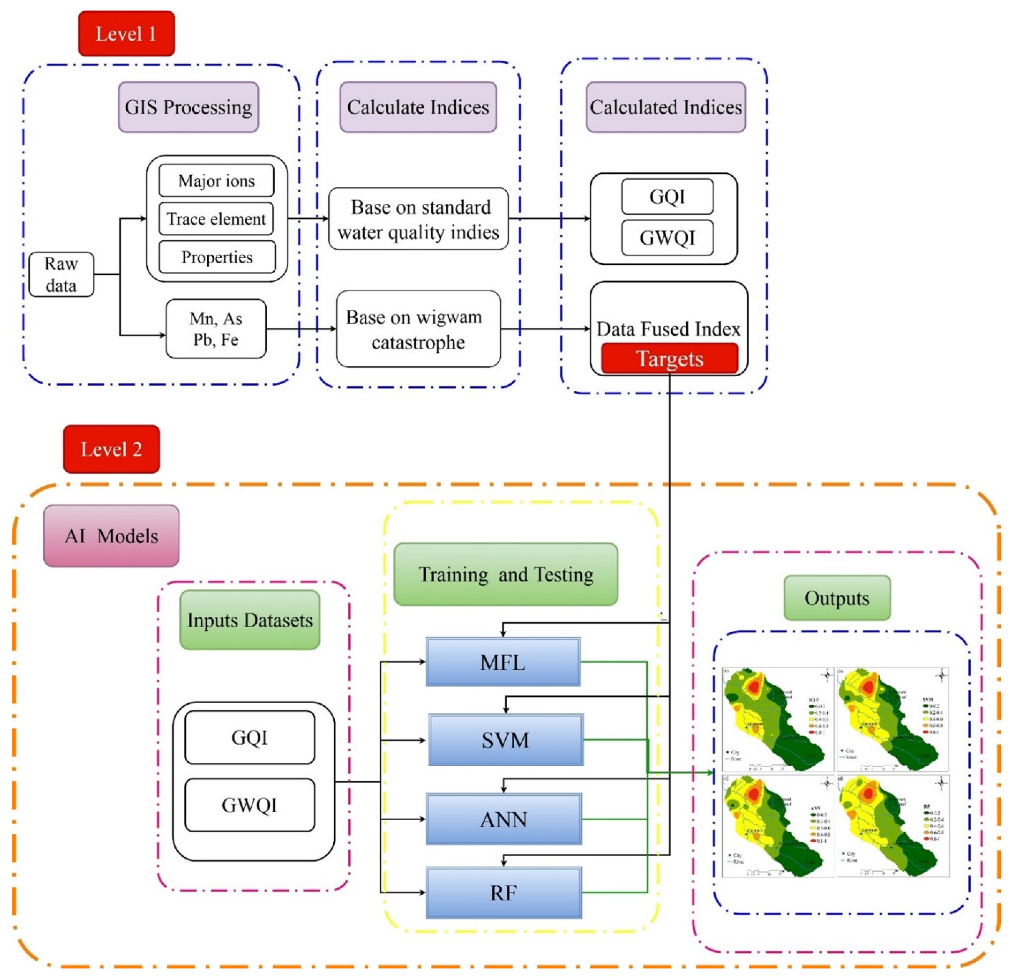
:The study of groundwater quality is typically conducted using water quality indices such as the Groundwater Quality Index (GQI) or the GroundWater Quality Index (GWQI). The indices are calculated using field data and a scoring system that uses ratios of the constituents to the prescribed standards and weights based on each constituent’s relative importance. The results obtained by this procedure suffer from inherent subjectivity, and consequently may have some conflicts between different water quality indices. An innovative feature drives this research to mitigate the conflicts in the results of GQI and GWQI by using the predictive power of artificial intelligence (AI) models and the integration of multiple water quality indicators into one representative index using the concept of data fusion through the catastrophe theory. This study employed a two-level AI modeling strategy. In Level 1, three indices were calculated: GQI, GWQI, and a data-fusion index based on four pollutants including manganese (Mn), arsenic (As), lead (Pb), and iron (Fe). Further data fusion was applied at Level 2 using supervised learning methods, including Mamdani fuzzy logic (MFL), support vector machine (SVM), artificial neural network (ANN), and random forest (RF), with calculated GQI and GWQI indices at Level 1 as inputs, and data-fused indices target values derived from Level 1 fusion as targets. We applied these methods to the Gulfepe-Zarinabad subbasin in northwest Iran. The results show that all AI models performed reasonably well, and the difference between models was negligible based on the root mean square errors (RMSE), and the coefficient of determination (r2) metrics. RF (r2 = 0.995 and RMSE = 0.006 in the test phase) and MFL (r = 0.921 and RMSE = 0.022 in the test phase) had the best and worst performances, respectively. The results indicate that AI models mitigate the conflicts between GQI and GWQI results. The method presented in this study can also be applied to modeling other aquifers.
1. Introduction
In semiarid areas such as Iran, population growth and increased water demands have caused an increase in shortages of drinking water resources [1]. Groundwater is considered to be among the few reliable sources of drinking water, particularly in rural areas. Moreover, in the context of human life, groundwater plays an important role in the industrial, agricultural, and domestic sectors [2,3]. Considering its renewable and nonrenewable, systematic and variable nature, groundwater quality issues, in terms of the water quality index, require a detailed investigation which is a critical component of groundwater management and protection programs [4].
Over the past few years, different water quality indices have been utilized for water quality assessments. Table 1 lists different water quality indices that are used for water quality assessment. The Groundwater Quality Index (GQI) [5] and the GroundWater Quality Index (GWQI) [6] are two indicators that have gained popularity as tools for quantifying groundwater quality. However, the calculation of these indices has some drawbacks. Through the application of these indices, water quality is determined by the use of field data as well as the numerical power of an assessment system that compares individual constituents to prescribed standards and weighted averages based on the relative importance of each constituent. Several studies have been done on this subject, including research by [7], which showed that the main disadvantage of GQI and GWQI frameworks is subjectivity in their prescribed rate and weight values. They used fuzzification to eliminate flaws in the frameworks and make them more accurate. Moreover, each index has its own advantage, so developing a combined water quality index which includes both GQI and GWQI is necessary.
Data-fusion architecture is a platform that connects databases with the help of data fusion techniques to create an integrated water quality system. It is a mathematical method that functions as the basis for merging data from several sources (e.g., GQI and GWQI) into one and combines the information from low and high levels. Using three indices, namely the GQI, the GWQI, and the Data-Fusion Index, this paper establishes a comprehensive water quality index to assess the status of groundwater quality. It explores how to integrate data from multiple water quality indices into a single index for the purposes of safeguarding the environment. Therefore, two innovative practices are introduced in aquifer management practices: (i) the creation of an index merged from multiple data points; and (ii) the comparison of the models used in predicting the used index.
Artificial intelligence (AI) has recently made many advances in computational methods, such as knowledge-based systems, neural networks, neuro-fuzzy logic, and multi-level fuzzy logic, which are important when analyzing environmental issues [13]. Several AI-based approaches have been proposed to assess groundwater quality and human health to address the shortcomings of traditional approaches, including the inherent uncertainty of many of the parameters of water quality [7,14,15]. In general, artificial neural networks (ANN), Mamdani fuzzy logic (MFL), support vector machine (SVM), and random forest (RF) offer a promising approach for the development of environmental indices since they reflect human understanding and expert knowledge. They can also handle datasets that are nonlinear, uncertain, and ambiguous. The simplified and logical form of the water quality indicators makes them more understandable to non-experts, the public, and managers [1], but they must address at least four shortcomings to serve as reliable tools: (i) these indicators are qualitatively uncertain and inexact; (ii) indicators use prescriptive values based on expert judgment for calculation; (iii) parameters underlying these groundwater quality indicators are not selected and weighted appropriately; and (iv) indicators are not calibrated to accept a wide range of values. By utilizing AI to analyze input and output data, this paper aims to fill these gaps by accounting for the inherent uncertainty and imprecision of inputs and outputs, utilizing four AI models, MFL, SVM, ANN, and RF. Therefore, an AI-based method was utilized in this study to determine groundwater quality, which illustrates the overall quality of water based on a relatively easy-to-calculate method. To this end, the GWQI and GQI were used as the base, and other critical quality parameters (e.g., trace element content) were added to give a more comprehensive groundwater quality index. In addition to examining the performance of the indicators, a case study was conducted on the groundwater quality in the Zarin Abad plain, Iran.
The study area is in the Qizil Ozen subbasin, which drains into Zanjan Province, northwest Iran, where a limited number of samples have been taken, probably the only sample measurements available. The country typically does not have a strong practice of equitable planning that emphasizes participation through decision-making, as evidenced by the paucity of data. For decision-makers, therefore, the use of different maps of water quality can present a particular challenge. In this study, the authors present an analysis that argues that planning problems in the above example are quite common in countries with ineffective or no planning. The main objectives of this study were to: (i) investigate data-fused indices into a single representative index; (ii) apply AI practices to a new realm of research; and (iii) compare the functionality of MFL, SVM, ANN, and RF in predicting the data-fused water quality index.
2. Study Area
2.1. Study Area Description
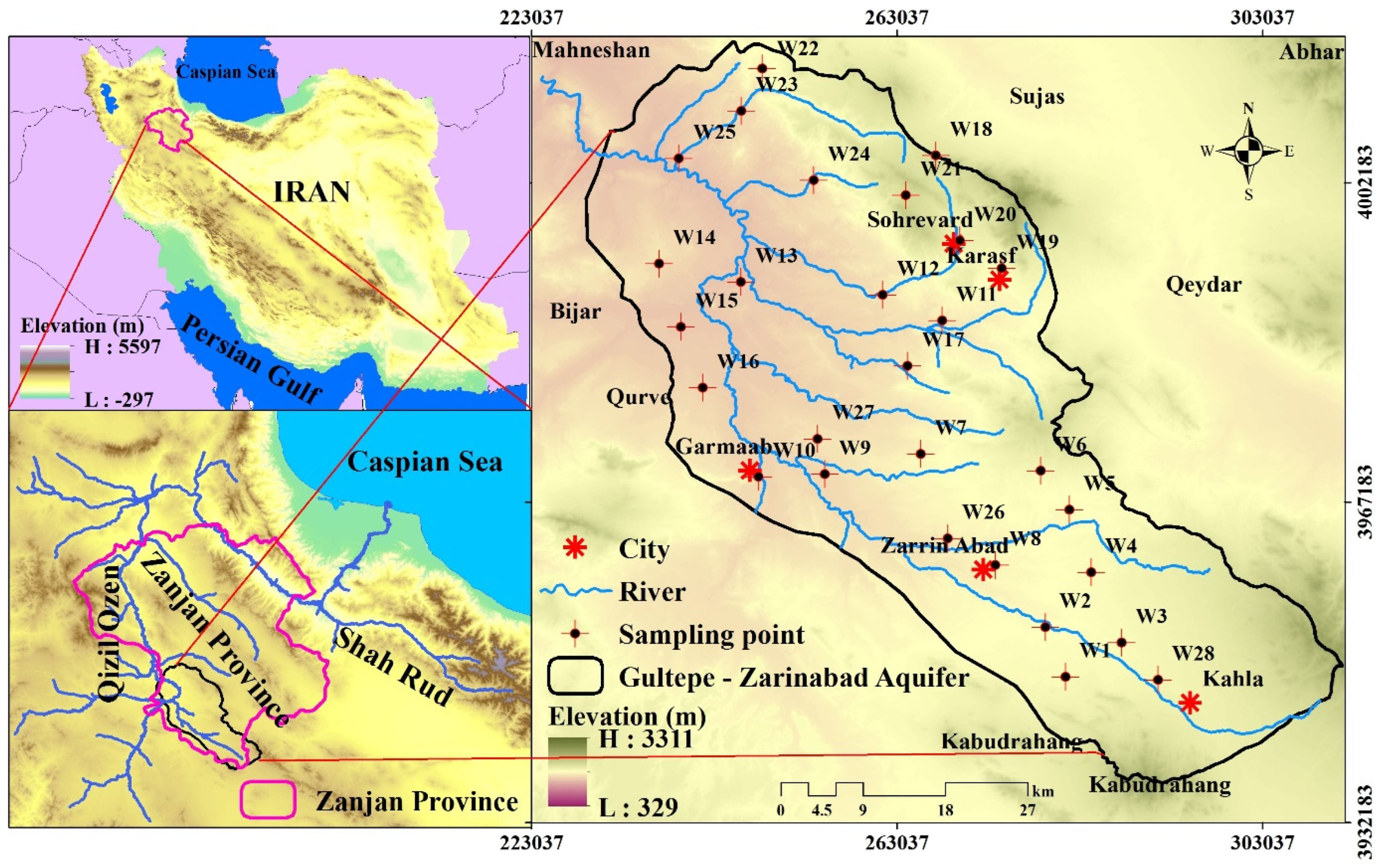
Gulfepe-Zarinabad subbasin lies in northwest Iran just along the Hamadan province border in the southwest Zanjan province, within the upper Qizil Ozen (Golden River) subbasin (Figure 1). The river, approximately 670 km long, drains Mount Qaflanti (Qaflankuh) at its upper end and empties into the Caspian Sea. The basin’s area is approximately 5124 km2, with 38% plains and 62% highlands. Over the past few decades, mining and agricultural activities have been prevalent in the study area.
Climate station data from Zanjan indicate a temperate climate with temperatures ranging from 3.6 °C in January to 21.8 °C in July. According to the De Martin approach, its climate is described as semiarid. The annual precipitation is 272 mm over a 20-year period (1985–2005). Rainfall is the major component of the wet season, peaking in November and December. Typically, rainfall is lowest in July and August, which corresponds to the dry season.
2.2. Geological Setting
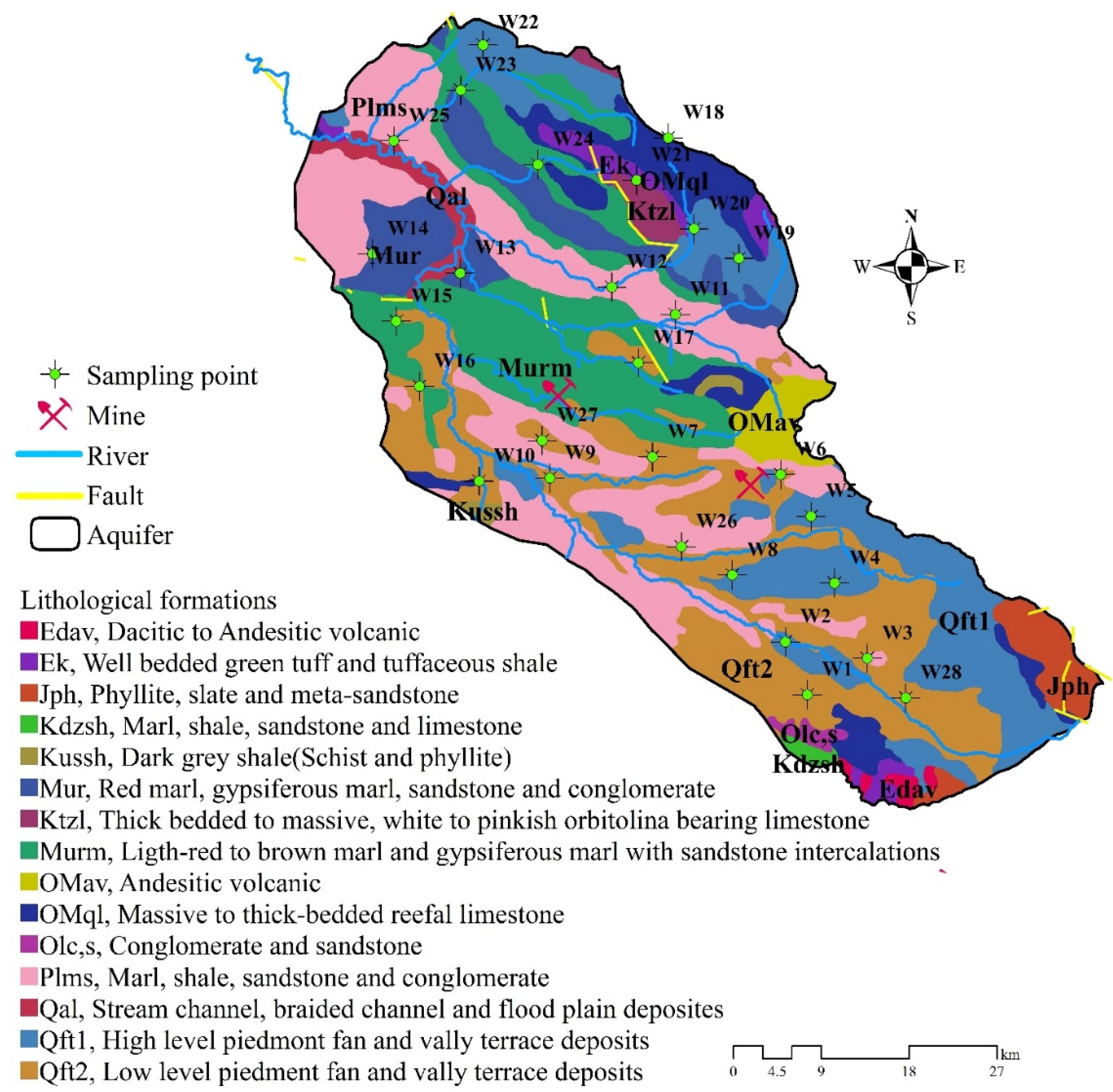
Located within Iran’s central tectonic zone, the Gultepe-Zarinabad subbasin consists of slate and schistose rocks which have undergone partial metamorphism during the Upper Triassic–Jurassic periods. A crystallized limestone can also be found between these rocks. Nayeen and Shemshak formations consist of low metamorphic rocks found in the plain. Conglomerate and sandstone are found at the base of Cretaceous rocks in the Albian, as well as andesite-basalt, Albian shale, and Upper Cretaceous shale, which is locally metamorphosed in the southern part of the region. The Tertiary rocks are characterized by their unconformities, made up of conglomerate and red sandstone, called Fajan formation, that date back to the Eocene age.
The southern parts of the island are dominated by volcanic rocks, including andesite-dacite-rhyolite, as well as green marl and sandstone. In the northern part of the state, the Upper Red Formation consists of marl, sandstone, and conglomerates interlayered with salt layers dating back to the Miocene. Clays and sands and their horizontal beddings form the Quaternary sediments of the plain’s central and western parts. Throughout the plain, Quaternary deposits (i.e., recent alluvium) predominate. Within these sediments, the study area developed an aquifer system with high transmissivity. Clay and sand with horizontal beddings are commonly found in Pliocene sediments in the upper Red Formation in the basin’s central and western parts.
2.3. Hydrogeology
The study area is the headwater subbasin of Qizil Ozen, a southernly flowing watercourse that collects tributaries from the highlands. Rivers originating in the study area receive tributaries, and more than ten watercourses feed into the main river (Figure 1). Although the river flowing through the study area is permanent, its tributaries are seasonal streams. The aquifer is therefore complexly interconnected with the rivers and streams of Gultepe-Zarinabad. Groundwater is extracted from the aquifer through several wells, springs, and qanats that are situated around the area (Figure 2).
The study area consists of an unconfined aquifer formed by alluvium of the Gultepe-Zarinabad plain. Across the region, the water table depth varies widely: it is relatively shallow near the Zarinabad River (6 m below ground), while it reaches 60 m or more in the eastern regions. The water table reaches its maximum level in April and May, and its minimum level in September and October. In the old part of the hills on the east and northeast, groundwater arises from the high ground and flows toward the plains, eventually emptying into the Zarinbad River.
A pumping test analysis determined that transmission varies from 30 to 900 m2/day within the study area. Transmissivity is lower in northeastern areas and higher in northern and northeastern areas. The boreholes are estimated to produce 30 to 120 m3/h of water. The lack of lithological information makes it difficult to inspect the subsurface geology, thus preventing the compilation of a comprehensive picture. However, geophysical data can help overcome these limitations. A maximum thickness of 181 m is recorded for the Gultepe-Zarinabad plain.
3. Data Preparation
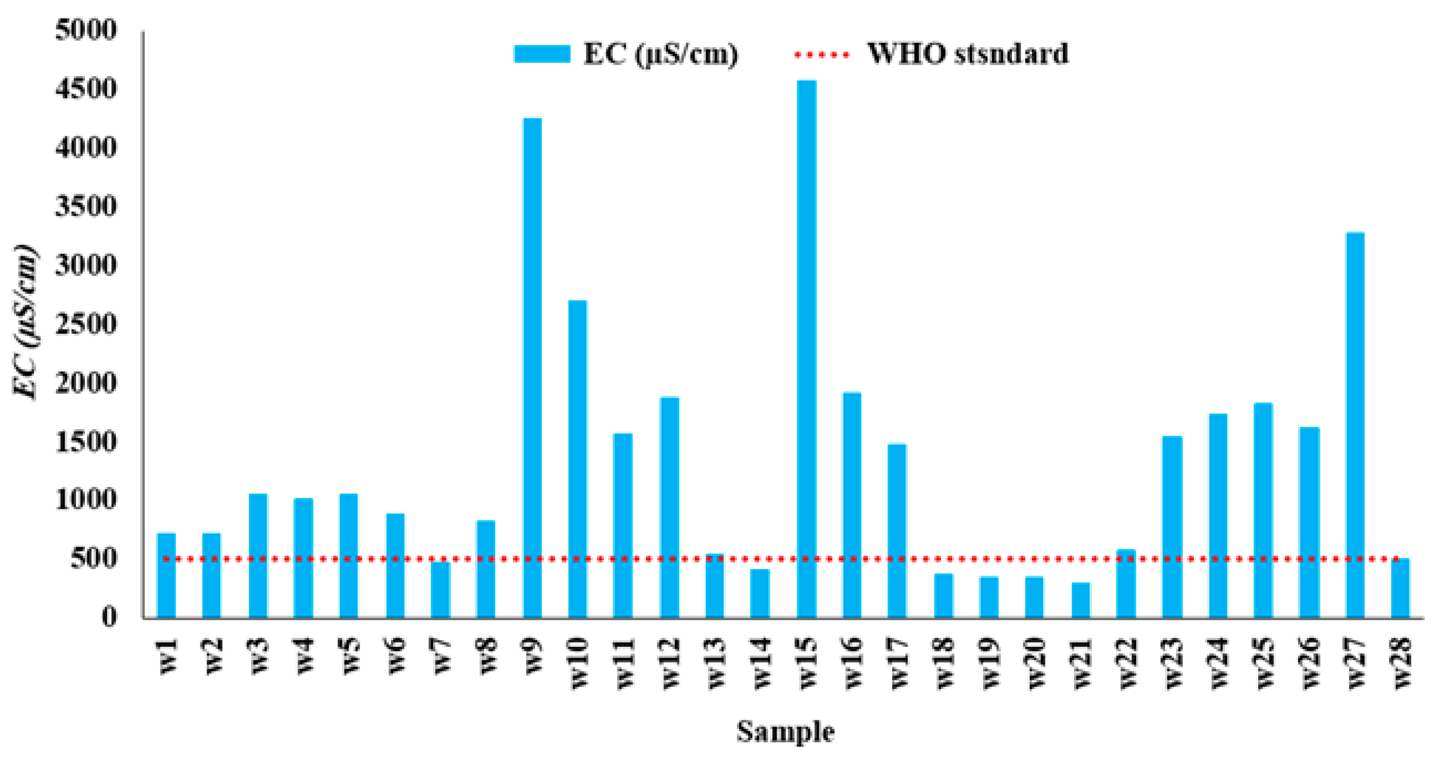
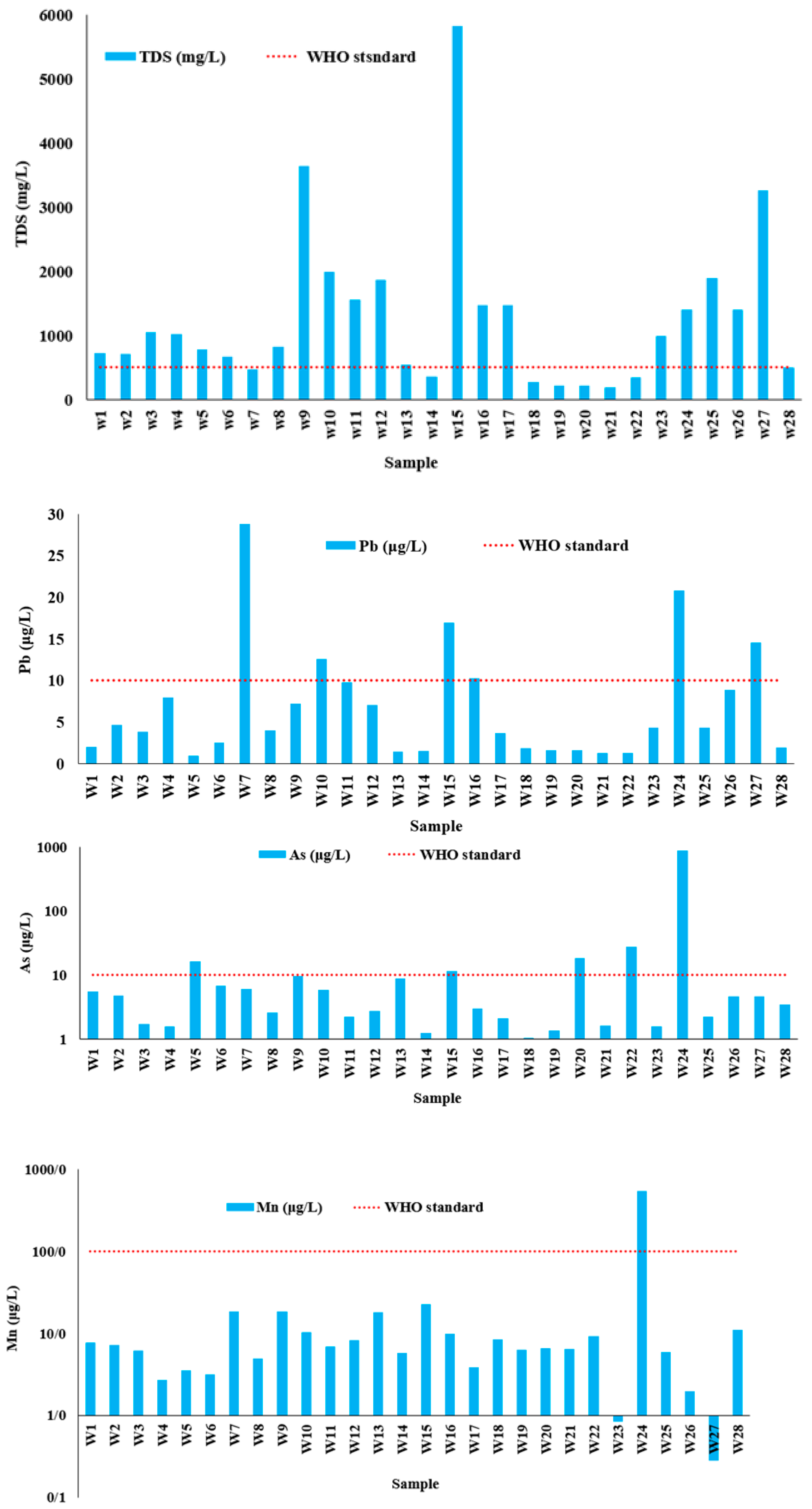
Following the guidelines of APHA (2005), the hydrogeological laboratory at the University of Hamadan measured major and minor ions, a set of trace elements, pH, and electrical conductivity (EC) of samples collected in 2019. In total 28 groundwater samples were analyzed and the analytical precision of each sample was calculated using a normalized inorganic charge balance (%CBE). Based on the results, all samples had a CBE of less than ±5%, defined as acceptable for groundwater studies [16]. A summary of groundwater quality parameters can be found in Table 2.
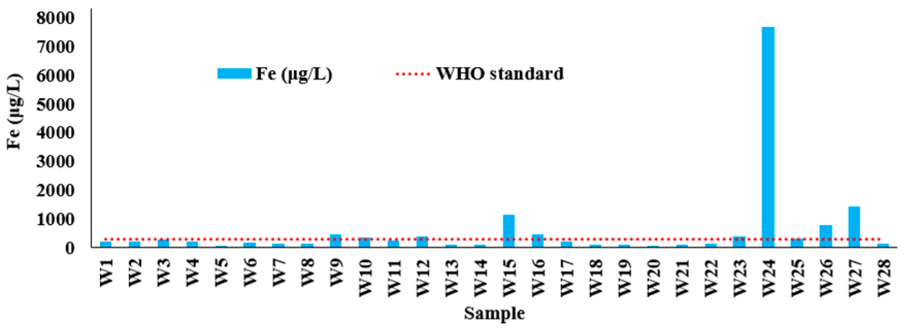
The measurements include physicochemical parameters (e.g., TDS, EC, and pH), major ions (e.g., SO42−, Na+, Ca2+, Mg2+, K+, HCO3−, and Cl−), and trace elements (e.g., Al, As, Cd, Cu, Cr, Fe, Mn, Ni, Pb, Co, and Zn). Table 2 lists the maximum admissible concentrations [17], which were exceeded in the cases of EC, TDS, TH, As, Fe, Pb, and Mn. Figure 3 shows the concentration of these parameters compared with their maximum permissible concentrations for the collected samples.
4. Methodology
Here we present the methodology for each of the three indices: GQI, GWQI, and Data-Fusion Index. Using the modeling strategy outlined in this section and illustrated in Figure 4, MFL, SVM, ANN, and RF were employed. In addition to calculating the three indices, the modeling strategy included the application of the data fusion technique to model the data-fused index. The ‘data-fused index’ strategy is suggested as a technique to explain the complexity of multiple water quality indicators, particularly in countries with limited planning experience. The data-fused index seeks to capture the most relevant signals across multiple water quality indicators. This paper presents several basic index-producing techniques which are described below.
4.1. Spatial Modeling
We present here an overview of the spatial distribution technique used by all the water quality indices in the paper. In terms of the spatial distribution of the water quality index values, two approaches can be used: (i) each sampling point is distributed over a grid, and the interpolated value of each pollutant is calculated pixel by pixel. The spatial representation of the contaminants is then obtained through calculations at each pixel; (ii) subsequent to calculating the indices at each observation well, the spatial distribution of the indices is mapped through spatial interpolation. The second strategy was used in the study. Using the four models strategy discussed in Section 4.5, spatially distributed values were then used.
Kriging interpolation was employed in this study, which is a statistical technique compared to other interpolation techniques (e.g., nearest point or moving average). The point values (in this case, those at observation wells) were used to calculate a weighted average function, in which the output of each pixel is equal to the product of its point values and weights, multiplied by the sum of those weights. In the Kriging method, weight factors are determined using a semivariogram model that is produced by generating spatial correlation information from pattern analysis [19].
4.2. Groundwater Quality Index (GQI)
To evaluate the utility of aquifer water as a drinking water source, the GQI is used. Mathematically, it is similar to the DRASTIC groundwater vulnerability index, developed by [20] proposed the GQI, which is based on the WHO (2011) water quality standards and combines different available water quality data. Further information can be found in [21]. The GQI framework is more objective than DRASTIC because it contains observed sample data from published standards rather than prescribed values. By using this index, one can determine the level of overall water quality through the spatial variation of contaminants, taking into account the environmental conditions, such as physical, chemical (e.g., Cl−, Na+, and Ca2+) and biological factors, in comparison to the standards established by the WHO (2011).
In a four-stage process, we performed the following steps: (i) calculate the C index using the measured concentrations and WHO drinking water standard (see Equation (1)); (ii) determine ratings (r) between 1 and 10 using Equation (2); (iii) evaluate the weights (w) using Equation (3); and (iv) determine GQI using r-ranks and w-weights for each variable and data layer (see Equation (4)). These are summarized as follows:
where at each observation well, Xr represents the measured concentration; X represents the maximum permissible level, as defined by the WHO (2011). The r expresses the contamination rate (1–10) and is calculated by Equation (2); and w reflects the relative weights of each index (Equation (3)). If the weight value for carcinogenic elements is ≤8, the calculated weight must be increased by 2. As shown in Equation (4), N is the total number of parameters evaluated in the suitability analysis. Note that the value of C in Equation (1) is set to 1 for a minimum impact on groundwater quality, 10 for a maximum impact, and 5 for the median impact. In general, GQI varies between 1 and 100, but can also exceed it. A value closer to 1 suggests poor water quality, while a value closer to 100 represents good quality water.
C = (Xr − X)/(Xr + X)
r = 0.5 × C 2 + 4.5 × C + 5 (r is between 1–10)
w = the mean rating value, r (of each layer)
w = the mean rating value, r (of each layer)
w (for non-carcinogenic elements (r ≤ 8)) = the mean rating value r + 2 (r ≤ 8)
4.3. GroundWater Quality Index (GWQI)
The GWQI, introduced by [6], is the second water quality index based on the WHO drinking standard used in this study. Although GWQI takes a different approach to water quality, it essentially follows a similar trajectory in terms of its suitability for drinking. Typically, the GWQI is calculated for determining whether groundwater is suitable for drinking [22] and it uses the weighted arithmetic index method [23,24,25,26] as follows:
- 1.
- Using the expert opinion, assign weights, to elements (i) of drinking water constituents, from 1 to 5 based on their respective weights. These values are listed in Table 3.
- 2.
- Determine the relative weight, Wi, for n, the number of elements, using the following equation:
- 3.
- Describe the quality rate, for the constituent as its concentration, , multiplied by 100 at each observation well, , which can be found in the WHO guidelines for drinking water, expressed as follows:
- 4.
- Using the subindex, , GWQI can be calculated as follows:the GWQI is another objective index, which is also scored using rates and weights, in the same manner as the DRASTIC vulnerability index. Table 3 lists the standard values S for the GWQI. In general, the GWQI ranges between 1 and 100, although it may exceed 100 in some cases. An index value closer to 1 represents good water quality, whereas an index value closer to 100 indicates poor water quality.
4.4. Data Fusion
A data-fusion approach was incorporated into the paper’s modeling strategy. As an umbrella term, it refers to the methods of combining variables or data to improve the quality of analysis, reduce uncertainty, or uncover new information. The practice of data fusion, which is used widely in electrical engineering, is defined by [27] as the combining of information from multiple sources. In 2011, [28] described fusion as low-level fusion, medium-level fusion, high-level fusion, and multi-level fusion.
Data fusion can be performed using several methods, including statistical matching, Bayesian inference (represented in [29], moving average filters (represented in [30], and gray relational analysis (represented in [31]. The parameters for trace metals (e.g., Mn, As, Pb, Fe), as the groundwater pollutants in the aquifer, were merged into a single output (i.e., target variable for AI models) using a data fusion approach in this study, as illustrated in Figure 4 and described below.
4.5. Artificial Intelligence
In this study, four different AI models, Mamdani fuzzy logic (MFL), support vector machine (SVM), artificial neural network (ANN), and random forest (RF), were used for developing the water quality index (i.e., GQI and GWQI)-based models. These AI models are described as follows.
4.5.1. Mamdani Fuzzy Logic (MFL)
By utilizing the fuzzy sets theory developed by [34], FL models enable relationships to be constructed between input and output data. The fuzzy sets can contain either 0 or 1 membership. Unlike classical set theory, the fuzzy set theory does not require sharp boundaries, and membership of objects does not refer to affirmation or rejection, but is generally a matter of degree rather than affirmation or rejection [35]. The exact value of 0 represents a total denial of membership, while 1 represents an affirmation of membership [36]. An MFL model can be described as follows: (a) output membership functions have fuzzy properties when using the “min” operation; (b) rules are determined through clustering by the FCM method [37]. The fuzzy implication operations in LFL are similar to those in MFL, but the product operator is used instead of the permutation operator [38]. Since water quality parameters are uncertain, calculating the nonlinear output may be more effective using a membership function [39].
4.5.2. Support Vector Machine (SVM)
In machine learning, the term SVM refers to statistical machine learning [40], a kernel-based learning approach. To map data in this method, high-dimensional hypothesis space is used (also known as feature space). In this model, prediction is implemented as a supervised model (similar to neural networks with similar weights and biases) [41]. This method can be applied in several ways, including predicting GWQI values (Table 1). GWQI and GQI data layers serve as inputs to the SVM. Then, a regression is established using the target value data-fused index (see Section 4.4). Based on radial basis functions (RBF), the SVM estimator mode specifies values for the SVM parameters, similar to [42]. It is composed of two parameters (γ and σ) embedded in its kernel, and their values are derived by applying the maximum likelihood approach [12]. The principles and mathematical equations entailed in SVR have been described in numerous papers and books [43,44]; therefore, these are not given in this paper.
4.5.3. Artificial Neural Network (ANN)
An ANN is specified here because its wide application makes it useful. In an ANN, a set of neurons transforms analog data into digital signals by converting it from analog to digital. There is no direct communication between the neurons in one layer, but they are in contact with the neurons in the layers below. Brain-like mechanisms mimic their functioning mathematically by fitting them with polynomials with activation functions as weights [44]. Our study employs a multilayer feedforward perceptron (MLP) network consisting of an input layer, a hidden layer, and an output layer. A trial-and-error approach was used to evaluate various alternatives for input-hidden and hidden-output layers [45]. The best activation functions for both input layers and hidden layers were found to be a ‘tangent sigmoid’ and a ‘linear’ function, respectively. The gradient descent, conjugate gradient, Levenberg–Marquardt, and other learning algorithms can be used for training the MLP model [46]. Here, we used Levenberg–Marquardt for training the MLP model.
4.5.4. Random Forest (RF)
In 2001, Breiman developed an ensemble machine learning technique called RF which is based on the concept of ‘bagged’ trees. Its application to GWQI is provided in Table 1. RF does not only allow the identification of linear and nonlinear relationships between variables but can also be used to attain classification and regression objectives [47]. A regression objective, such as the conditional mean of a dependent variable, can be effectively produced with RF. Using this method, multiple decision trees are gathered, and then the predictions are averaged and obtained through multiple decision trees through bootstrap aggregation [48]. In this study, the model was formed as a supervised prediction model based on the two layers of data, GQI and GWQI. By connecting multiple inputs and outputs to binary classification, a forest of regression trees was derived by applying bagging [49] and random subspace to develop weak learners. The mean squared error of a classification model determines prediction errors. More details on RF can be found in [50].
4.6. Normalization of Indices
Data fusion transforms each index value into a set of indices ranging from 0 to 1, where 0 reflects the lowest risk and 1 indicates the highest risk. By definition, their least desirable values occur at the lower values of the GWQI indices; thus, further transformation is taken into account. Accordingly, the following normalization schemes are employed:
where i denotes the number of data points; Xmin and Xmax are minimum and maximum index values, respectively; Xr represents the normalized index and is treated as a variable.
4.7. Modeling Strategy
According to Figure 4, the AI modeling strategy in this study involved activities at two levels, in addition to those at Level 1.
4.7.1. Level 1: Calculating the Index Values
Typically, three indices (e.g., GQI, GWQI, and the data-fusion index) are calculated and used to evaluate the water quality.
4.7.2. Level 1: Data Fusion
The four trace elements Mn, As, Pb, and Fe were transformed into a single data-fusion index at Level 1 using Equation (9), resulting in the index at Level 1. Choosing the index order was, however, necessary for this.
Expert opinion determines how each index is weighted, in terms of the root of the function in Equation (9). As was given more weight than other elements due to its significance. Then Pb was given a lower weight.
At Level 1, the indices were normalized from 0 to 1, to minimize the effect of scale. The GWQI indexes were normalized by Equation (10), while the GQI index was normalized by Equation (11).
4.7.3. Level 2: Further Fusion Strategies
The next level of data fusion required supervised learning via MFL, SVM, ANN, and RF, incorporating AI models. Both of these models used Level 1 indices as inputs, and their target values are derived from Level 1 fusion.
4.8. Model’s Performance Evaluation and Banding Spatial Results
For Level 1, there was no need to calculate performance metrics. However, using the ROC/AUC algorithm, the efficiency of the relevant indices at Levels 1 and 2 could be examined. ROC is commonly employed for spatial goodness-of-fit calculations. This analysis method for radar images is called “signal detection theory” which enables us to tell whether a blip emanates from a friendly ship, an enemy target or noise. As a measure of accuracy, AUC is measured from 1 to 0.55, and a value of 1 indicates perfect accuracy, while a value of 0.5 indicates the presence of significant noise.
Best practices were followed to construct the ANN models, which allowed the number of neurons from 1 to 100 to be varied by trial and error at the hidden layer. The error functions were calculated as the root mean square errors (RMSE), and the correlation coefficient (CC) or the coefficient of determination (r2) was calculated for each run. The best ANN model was selected based on the neurons with the lowest RMSE value. In the training phase, 80% of the data points were randomly selected, while the remaining 20% were selected for the testing phase for the MFL, SVM, ANN, and RF models.
At Level 1, models were evaluated to determine if they were appropriate for the objective, while at Level 2, a model’s robustness was determined. At Level 2, performance was determined by calculating the CC and RMSE. CC values range from 1 to -1, with values near 1 indicating near-perfect performance, while values near zero indicate poor correlations. The root mean square error scales range from 0 (i.e., the ‘perfect model’) to any other real number. This is a measurement of how closely observed results match those of the models.
Using the normalized indices, results were banded according to the following: Band 0–0.2 (low risk), Band 0.2–0.4 (relatively low risk), Band 0.4–0.6 (moderate risk), Band 0.6–0.8 (relatively high risk), Band 0.8–1 (high risk).
The ROC/AUC metrics at Levels 1 and 2 were based on the comparison of two similar distributions of the modeled indices to the observed (target) indices to evaluate false negatives and true positives. Despite the lack of an ideal value, certain tests were conducted in order to select an appropriate comparison. These tests were 0.2, 0.4, 0.6, and 0.8. We will discuss this in more detail later.
5. Results
5.1. GQI and GWQI
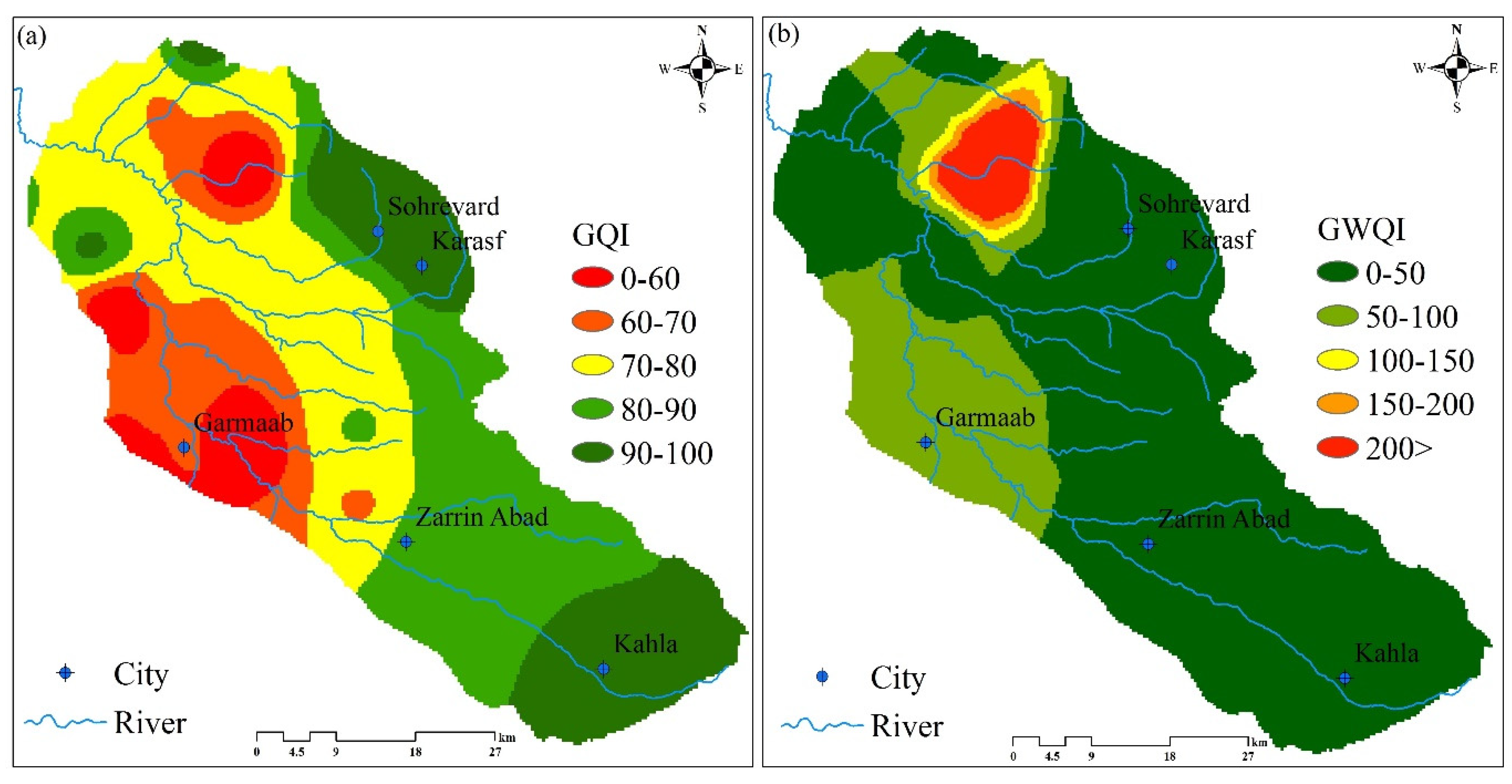
Each water quality index was determined based on the GQI and GWQI using Equations (1) and (2) and the results were spatially distributed based on the IDW interpolation method. Using the visual color coding system, the results were divided into five bands, in which the color red corresponded to low quality and the color green corresponded to high quality. A GQI with a lower value corresponds to lower water quality, but a GWQI with a higher value represents lower water quality. There were some similarities and conflicts between the spatial pattern of GQI (Figure 5a) and GWQI (Figure 5b), outlined as follows. In the northern areas of the plain, an area with poor quality water was similar to that found in GQI and GWQI. Moreover, substantial conflicts were also observed between the two indices in the southwest regions, where GQI identified these areas with the lowest quality, but GWQI did not. The central part of the plain was also characterized by GQI as in a moderate band, but it was within a high-quality band.
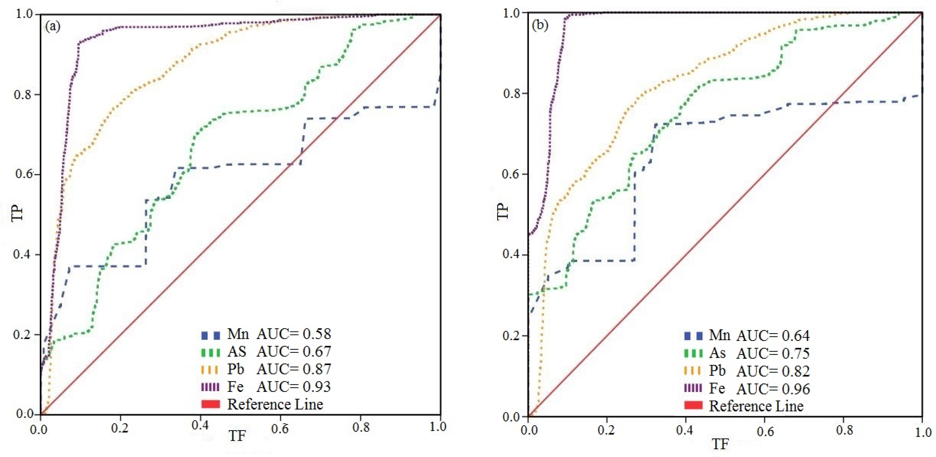
Figure 6 illustrates with ROC curves and AUC values the performance of GQI (Figure 6a) and GWQI (Figure 6b). The curves in this figure are plotted versus four trace metals: Mn, As, Pb, and Fe. Unlike their visual comparison of spatial patterns, the AUC values in Figure 6 indicate that there were no significant differences between AUC values. In terms of Mn, As, and Fe, GWQI outperformed GQI, but GQI was superior in Pb.
5.2. Water Quality Index Based on AI Models
The visual comparison between GQI and GWQI and also their quantitative assessment by the ROC curve show the necessity to develop new indices that mitigate spatial conflicts between GQI and GWQI. Hence, a set of AI models were formulated to develop new indices, and the results are presented as follows.
5.2.1. Results of Training and Testing
The AI models were formulated according to the modeling procedure described in Section 2. The configurations are outlined as follows:
MFL—A Gaussian membership function was used to create five input and output clusters. We selected the best cluster number based on RMSE by considering different cluster numbers ranging from 1 to 35. The number of input and output data clusters contributes to the number of if-then rules.
SVM—Radial basis function (RBF) was incorporated with the regularization parameter (C) equal to 20 and the kernel width (γ) equal to 0.5.
ANN—The input and hidden layers were optimally activated using the hyperbolic tangent sigmoidal and linear functions, respectively. The hidden layer contained four neurons, and the output layer contained one neuron. A total of 600 training epochs were performed.
RF—The number of trees (nt) was 1500, and the number of variables (nv) was 11.
Table 4 summarizes the results of the training and testing phases of AI models, in terms of r2 and RMSE. According to the results of the test phase, RF (r2 = 0.995 and RMSE = 0.006) had the highest performance, followed by ANN (r2 = 0.943 and RMSE = 0.020), SVM (r = 0.941 and RMSE = 0.021), and MFL (r2 = 0.921 and RMSE = 0.022). Compared to the training phase, the performance of the models was slightly lower in the testing phase.
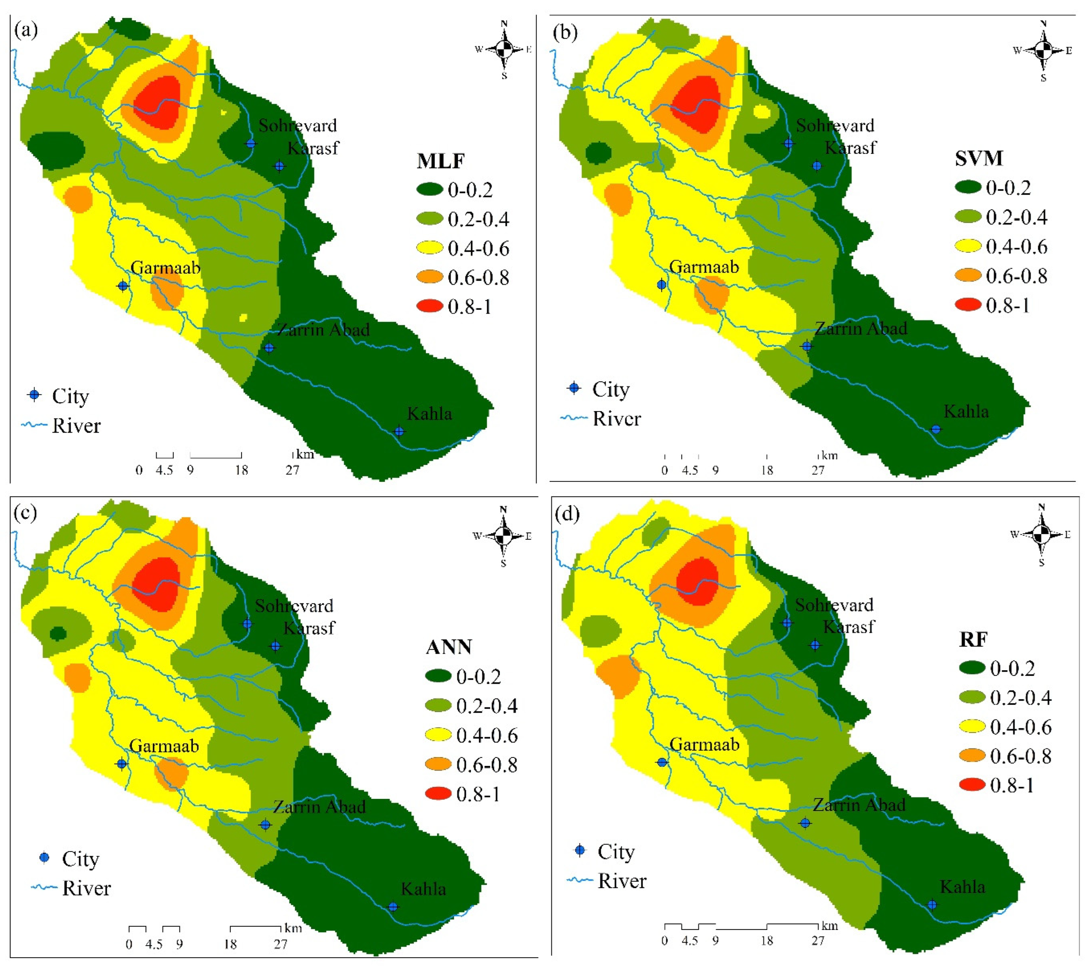
5.2.2. Results of AI-Based Water Quality Index Mapping
Based on AI models, Figure 7 illustrates the spatial distribution of water quality indices. Overall, all models produced similar spatial patterns; however, there were some differences. Note that the figure is divided into five equal bands, where Bands 1 to 5 correspond to high and low water quality, respectively. Northern parts of the plain have poor water quality, whereas southern parts of the plain have good water quality. Among the AI modes, only the MFL model identified the central parts as bands with relatively good water quality. According to Figure 4 and Figure 7, AI models are capable of incorporating both characteristics of GQI and GWQI in order to develop new water quality indices. Based on AI models, the southeastern parts of the plain fall into Bands 3 and 4 (poor and moderate water quality under the influence of GQI). Notably, these areas are not included in Bands 4 and 5 in the GWQI.
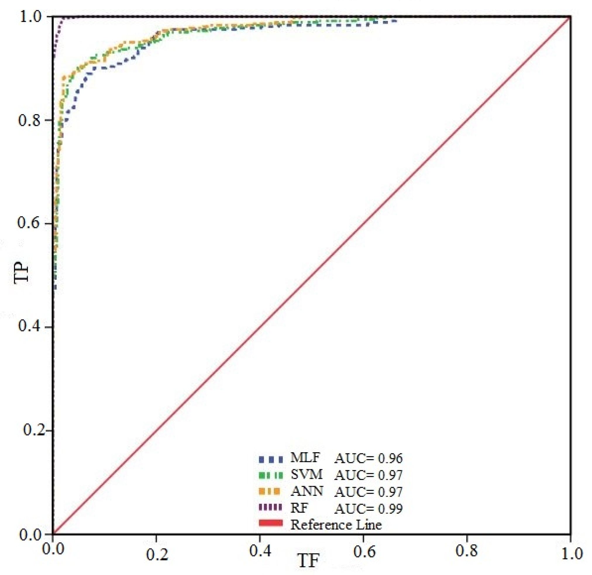
Figure 8 illustrates ROC curves which evaluate the performance of AI models and show that all the models were relatively similar in their performances and the difference between the performances of different models was not statistically significant. Meanwhile, RF and MFL had the highest and lowest performances, respectively. SVM and ANN had nearly identical performances. It is once again impossible to rank the models by their performance because there was no significant difference between them.
6. Discussion
In this study, GQI and GWQI were compared as two commonly used water quality indices, and significant differences between them were found despite some similarities. Differences in the results of GQI and GWQI were due to inherent subjectivity within prescribed rates and weights included in the calculation procedures [50]. Since the worst water quality was identified based on GQI, southwest parts of the study area have a significant difference. Comparatively, these regions have the best water quality based on GWQI. However, there are also some similarities in the water quality in the northern parts of the study area. To mitigate these conflicts, the paper proposes an AI-based index.
In previous studies, a variety of strategies has been used to decrease subjectivity, including (i) fuzzification of GQI and GWQI frameworks [1,51], (ii) identifying weight values using removal and sensitivity analysis [5], and (iii) defining the maximum allowable levels as a threshold of safety instead of a single value [51]. Among these strategies, the literature highlights AI models as an appropriate technique to decrease inherence subjectivities [5]. In this context, the current study proposes a new AI-based methodology that maximizes model performance by reducing inherent subjectivity.
In terms of the ROC curve, four AI models (e.g., MFL, SVM, ANN, RF) showed significant improvements compared to typical GQI and GWQI frameworks. However, there were marginal differences between the outcomes of AI models. Considering AI models are case-intensive and their performances rely heavily on the data, some multiple modeling strategies can be used to achieve further improvements [52]. Yet, such strategies are not necessary since all AI models are identical and have greater accuracy.
A decision support system can be employed to manage groundwater resources based on the results of the study. In the northern parts of the study area, some remedial strategies could be beneficial in hotspots (Bands 4 and 5). In addition, regular monitoring of water quality is necessary for other regions (Bands 1 to 3) to prevent water quality degradation. Beyond aquifer vulnerability, these results provide a deeper understanding of aquifer management, and future investigation is recommended.
As far as the authors are aware, there are no previously collected historical data on aquifer water quality for the study area, which is one of the limitations of this study. As a result, the results cannot be objectively compared with established baselines, which entails the inability to make objective comparisons based on the data. Although farming and mining activities are ongoing within the study area, both are considered to be contemporary and have only existed since the late 1990s when the baseline conditions were considered sustainable and risk-free. As a result of the results presented in this study, we can conclude that there is a serious problem with water quality in the study area, and this issue might even become worse in the future if the same practices are continued. There are a number of reasons why the problem arises, including the lack of proper environmental planning and management in the study area and poor planning practices throughout the country in general.
A larger sample size is believed to result in a more precise outcome for AI methods such as tree-based models (e.g., RF), though some experts believe that they are less sensitive to the number of samples [53]. Therefore, it is recommended to explore other AI models such as eXtreme gradient boosting in developing the fusion-based water quality index. According to conventional water quality indices, each water quality parameter is given a constant weight regardless of the hydrogeological characteristics of the area, and these weights are used to assess the water quality of all aquifers, resulting in uncertainty. While AI models can reduce the uncertainty of conventional water quality indices, since they are black box models, they are unable to suggest new weight scores for each water quality parameter. However, the level of uncertainty associated with the developed AI models can be reduced by using cross-validation and hyperparameter tuning procedures during the model’s training process [54].
7. Summary and Conclusions
This study formulates a methodology based on AI models to decrease the inherent subjectivity and possible conflicts in the water quality indices of GQI and GWQI. Notably, the basic frameworks to calculate GQI and GWQI suffer from inherent subjectivity, which can produce substantial conflicts between the spatial patterns of results. An AI modeling strategy based on two levels was used in this study. Three indices were calculated in Level 1: GQI, GWQI, and a data-fusion index based on four trace elements, Mn, As, Pb, and Fe by the catastrophe theory. Further data fusion was applied at Level 2 using supervised learning methods, MFL, SVM, ANN, and RF, with calculated GQI and GWQI indices at Level 1 as inputs, and data-fused indices target values derived from Level 1 fusion as targets. This formulation was applied to the Gulfepe-Zarinabad subbasin in northwest Iran, and a substantial conflict was observed in the spatial pattern of GQI a GWQI. By implementing the AI-based formulation, the conflicts between GQI and GWQI were substantially mitigated, and the performance of modeling was improved regarding the ROC curve and the AUC values in all AI models. There was a marginal difference between developed AI models. A comparison of the test phase results showed that RF (r2 = 0.99 and RMSE = 0.006) had the best performance, while MFL (r2 = 0.921 and RMSE = 0.022) had the worst performance. The southeastern parts of the plain, based on the AI models, were classified into Bands 3 and 4, respectively, indicating poor and moderate water quality under the influence of GQI in those areas. The GWQI does not include these areas in Bands 4 and 5 as they are not considered high-quality areas.
Author Contributions
Conceptualization, A.A.N.; methodology, R.B.; software, A.A.R.; validation, A.A.N. and R.B.; formal analysis, S.S.; investigation, and resources, A.A.N.; data curation, A.A.R.; writing—original draft preparation, A.A.R.; writing—review and editing, R.B.; visualization, S.S.; supervision, A.A.N.; project administration, S.S. All authors have read and agreed to the published version of the manuscript.
Funding
This research received no external funding.
Data Availability Statement
Data is available based on the request.
Conflicts of Interest
The authors declare no conflict of interest.
References
- Gharibi, H.; Mahvi, A.H.; Nabizadeh, R.; Arabalibeik, H.; Yunesian, M.; Sowlat, M.H. A novel approach in water quality assessment based on fuzzy logic. J. Environ. Manag. 2012, 112, 87–95. [Google Scholar] [CrossRef] [PubMed]
- Sharma, S.; Nagpal, A.K.; Kaur, I. Appraisal of heavy metal contents in groundwater and associated health hazards posed to human population of Ropar wetland, Punjab, India and its environs. Chemosphere 2019, 227, 179–190. [Google Scholar] [CrossRef] [PubMed]
- Razzagh, S.; Nadiri, A.A.; Khatibi, R.; Sadeghfam, S.; Senapathi, V.; Sekar, S. An investigation to human health risks from multiple contaminants and multiple origins by introducing ‘Total Information Management’. Environ. Sci. Pollut. Res. 2021, 28, 18702–18724. [Google Scholar] [CrossRef] [PubMed]
- Chen, W.; Li, H.; Hou, E.; Wang, S.; Wang, G.; Panahi, M.; Li, T.; Peng, T.; Guo, C.; Niu, C.; et al. GIS-based groundwater potential analysis using novel ensemble weights-of-evidence with logistic regression and functional tree models. Sci. Total Environ. 2018, 634, 853–867. [Google Scholar] [CrossRef] [Green Version]
- Babiker, I.S.; Mohamed, M.A.A.; Hiyama, T. Assessing groundwater quality using GIS. Water Resour Manag. 2007, 21, 699–715. [Google Scholar] [CrossRef]
- Ribeiro, L.; Paralta, E.; Nascimento, J.; Amaro, S.; Oliveira, E.; Salgueiro, R. A agricultura a delimitac ao das zonas vulnera’veis aos nitratosdeorigem agrı’cola segundo a Directiva 91/676/CE. In Proceedings of the III Congreso Ibe’rico Sobre Gestio’n e Planificacio’n del Agua; Universidad de Sevilla: Sevilla, Spain, 2002; pp. 508–513. [Google Scholar]
- Vadiati, M.; Asghari-Moghaddam, A.; Nakhaei, M.; Adamowski, J.; Akbarzadeh, A.H. A fuzzy-logic based decision-making approach for identification of groundwater quality based on groundwater quality indices. J. Environ. Manag. 2016, 184, 255–270. [Google Scholar] [CrossRef] [PubMed]
- Elbeltagi, A.; Pande, C.B.; Kouadri, S.; Islam, A.R.M. Applications of various data-driven models for the prediction of groundwater quality index in the Akot basin, Maharashtra, India. Environ. Sci. Pollut. Res. 2021, 29, 17591–17605. [Google Scholar] [CrossRef] [PubMed]
- Brahim, F.B.; Boughariou, E.; Bouri, S. Multicriteria-analysis of deep groundwater quality using WQI and fuzzy logic tool in GIS: A case study of Kebilli region, SW Tunisia. J. Afr. Earth Sci. 2021, 180, 104224. [Google Scholar] [CrossRef]
- Singha, S.; Pasupuleti, S.; Singha, S.S.; Singh, R.; Kumar, S. Prediction of groundwater quality using efficient machine learning technique. Chemosphere 2021, 276, 130265. [Google Scholar] [CrossRef] [PubMed]
- Trabelsi, F.; Ali, S.B.H. Exploring Machine Learning Models in Predicting Irrigation Groundwater Quality Indices for Effective Decision Making in Medjerda River Basin, Tunisia. Sustainability 2022, 14, 2341. [Google Scholar] [CrossRef]
- Yu, P.S.; Yang, T.C.; Chen, S.Y.; Kuo, C.M.; Tseng, H.W. Comparison of random forests and support vector machine for real-time radar-derived rainfall forecasting. J. Hydrol. 2017, 552, 92–104. [Google Scholar] [CrossRef]
- Chau, K.W. A review on integration of artificial intelligence into water quality modelling. Mar. Poll. Bull. 2006, 52, 726–733. [Google Scholar] [CrossRef] [PubMed] [Green Version]
- Gharekhani, M.; Khatibi, R.; Nadiri, A.A.; Sadeghfam, S. Aggregating risks from aquifer contamination and subsidence by inclusive multiple modeling practices. In Risk, Reliability and Sustainable Remediation in the Field of Civil and Environmental Engineering; Elsevier: Amsterdam, The Netherlands, 2022; pp. 155–182. [Google Scholar]
- Nadiri, A.A.; Sedghi, Z.; Khatibi, R.; Gharekhani, M. Mapping vulnerability of multiple aquifers using multiple models and fuzzy logic to objectively derive model structures. Sci. Total Environ. 2017, 593, 75–90. [Google Scholar] [CrossRef]
- Hounslow, A.W. Water Quality Data: Analysis and Interpretation; Lewis Publisher: Boca Raton, FL, USA, 1995; p. 397. Available online: https://www.taylorfrancis.com/books/mono/10.1201/9780203734117/water-quality-data-arthur-hounslow (accessed on 10 September 2022). [CrossRef]
- WHO. Guidelines for drinking-water quality. In Recommendations, 3rd ed.; WHO: Geneva, Switzerland, 2011; Volume 1. [Google Scholar]
- Edmond, J.M.; Palmer, M.R.; Measures, C.I.; Grant, B.; Stallard, R.F. The fluvial geochemistry and denudation rate of the Guayana Shield in Venezuela, Colombia, and Brazil. Geochim. Cosmochim. Acta 1995, 59, 301–325. [Google Scholar] [CrossRef]
- Isaaks, E.H.; Srivastava, R.M. An Introduction to Applied Geostatistics Illustrated Edition; Oxford University Press: Oxford, UK, 1990. [Google Scholar]
- Aller, L.; Bennett, T.; Lehr, J.; Petty, R.; Hackett, G. EPA/600/2-87/035; US EPA/Robert S. Kerr Environmental Research Laboratory EPA: Ada, OK, USA, 1987. [Google Scholar]
- Rufino, F.; Busico, G.; Cuoco, E.; Darrah, T.H.; Tedesco, D. Evaluating the suitability of urban groundwater resources for drinking water and irrigation purposes: An integrated a proach in the Agro-Aversano area of Southern Italy. Environ. Monit. Assess. 2019, 191, 768. [Google Scholar] [CrossRef] [PubMed]
- Tiwari, T.N.; Mishra, M. A preliminary assignment of water quality index of major Indian rivers. Indian J. Environ. Prot. 1985, 5, 276. [Google Scholar]
- Adimalla, N.; Li, P.; Qian, H. Evaluation of groundwater contamination for fluoride and nitrate in semi-arid region of Nirmal Province, South India: A special emphasis on human health risk assessment (HHRA). Hum. Ecol. Risk Assess. Int. J. 2018, 25, 1107–1124. [Google Scholar] [CrossRef]
- Brown, R.M.; McClelland, N.I.; Deininger, R.A.; O’Connor, M.F. A Water Quality Index—Crashing the Psychological Barrier. Indicators of Environmental Quality; Springer: Berlin/Heidelberg, Germany, 1972; pp. 173–182. [Google Scholar]
- Horton, R.K. An index number system for rating water quality. J. Water Pollut. Control Fed. 1965, 37, 300–306. [Google Scholar]
- Ramakrishnaiah, C.R.; Sadashivaiah, C.; Ranganna, G. Assessment of water quality index for the groundwater in Tumkur Taluk, Karnataka State, India. E-J. Chem. 2009, 6, 523–530. [Google Scholar] [CrossRef] [Green Version]
- See, L.; Abrahart, R. Multi-model data fusion for hydrological forecasting. Comput. Geosci. 2001, 27, 987–994. [Google Scholar] [CrossRef]
- Abdelgawad, A.; Bayoumi, M. Sand monitoring in pipelines using Distributed Data Fusion algorithm. In Proceedings of the 2011 IEEE Sensors Applications Symposium, San Antonio, TX, USA, 22–24 February 2011; pp. 217–220. [Google Scholar]
- Endres, E.; Augustin, T. Statistical matching of discrete data by Bayesian networks. In Proceedings of the Eighth International Conference on Probabilistic Graphical Models, Lugano, Switzerland, 6–9 September 2016; Volume 52, pp. 159–170. [Google Scholar]
- Rodrígueza, S.; De Paza, J.F.; Villarrubiaa, G.; Zato, C.; Bajo, J.; Corchado, J.M. Multi-Agent Information Fusion System to manage data from a WSN in a residential home. Inf. Fusion 2015, 23, 43–57. [Google Scholar] [CrossRef]
- Huang, Y.P.; Chu, H.C. Simplifying fuzzy modeling by both gray relational analysis and data transformation methods. Fuzzy Sets Syst. 1999, 104, 183–197. [Google Scholar] [CrossRef]
- Hansson, S.O. Decision Theory, A Brief Introduction; Royal Institute of Technology (KTH): Stockholm, Sweden, 2005. [Google Scholar]
- Sadeghfam, S.; Mirahmadi, R.; Khatibi, R.; Mirabbasi, R.; Nadiri, A.A. Investigating meteorological/groundwater droughts by copula to study anthropogenic impacts. Sci. Rep. 2022, 12, 8285. [Google Scholar] [CrossRef]
- Zadeh, L.A. Fuzzy sets. Inf. Control. 1965, 8, 338–353. [Google Scholar] [CrossRef] [Green Version]
- Demico, R.V.; Klir, G.J. Fuzzy Logic in Geology; Elsevier Academic Press: San Diego, CA, USA, 2004; p. 347. [Google Scholar]
- Barzegar, R.; Moghaddam, A.A.; Baghban, H. A supervised committee machine artificial intelligent for improving DRASTIC method to assess groundwater contamination risk: A case study from Tabriz plain aquifer, Iran. Stoch. Environ. Res. Risk Assess. 2016, 30, 883–899. [Google Scholar] [CrossRef]
- Larsen, P.M. Industrial applications of fuzzy logic control. Int. J. Man-Mach. Stud. 1980, 12, 3–10. [Google Scholar] [CrossRef]
- Nadiri, A.A.; Moazamnia, M.; Sadeghfam, S.; Barzegar, R. Mapping Risk to Land Subsidence: Developing a Two-Level Modeling Strategy by Combining Multi-Criteria Decision-Making and Artificial Intelligence Techniques. Water 2021, 13, 2622. [Google Scholar] [CrossRef]
- Vapnik, V.N. Statistical Learning Theory; Wiley: Hoboken, NJ, USA, 1998. [Google Scholar]
- Gharekhani, M.; Nadiri, A.A.; Khatibi, R.; Sadeghfam, S.; Moghaddam, A.A. A study of uncertainties in groundwater vulnerability modelling using Bayesian model averaging (BMA). J. Environ. Manag. 2021, 303, 114168. [Google Scholar] [CrossRef] [PubMed]
- Nadiri, A.A.; Habibi, I.; Gharekhani, M.; Sadeghfam, S.; Barzegar, R.; Karimzadeh, S. Introducing dynamic land subsidence index based on the ALPRIFT framework using artificial intelligence techniques. Earth Sci. Inform. 2022, 15, 1007–1021. [Google Scholar] [CrossRef]
- Tien Bui, D.; Pradhan, B.; Lofman, O.; Revhaug, I. Landslide susceptibility assessment in Vietnam using support vector machines, decision tree, and naive Bayes models. Math. Probl. Eng. 2012, 2012, 974638. [Google Scholar] [CrossRef] [Green Version]
- Li, W.; Yang, M.; Liang, Z.; Zhu, Y.; Mao, W.; Shi, J.; Chen, Y. Assessment for surface water quality in Lake Taihu Tiaoxi River Basin China based on support vector machine. Stoch. Environ. Res. Risk Assess. 2013, 27, 1861–1870. [Google Scholar] [CrossRef]
- Sedghi, Z.; Rostami, A.A.; Khatibi, R.; Nadiri, A.A.; Sadeghfam, S.; Abdoallahi, A. Mapping and aggregating groundwater quality indices for aquifer management using Inclusive Multiple Modeling practices. In Risk, Reliability and Sustainable Remediation in the Field of Civil and Environmental Engineering; Elsevier: Amsterdam, The Netherlands, 2022; pp. 155–182. [Google Scholar]
- Nourani, V.; Mogaddam, A.A.; Nadiri, A.A. An ANN-based model for spatiotemporal groundwater level forecasting. Hydrol. Process. Int. J. 2008, 22, 5054–5066. [Google Scholar] [CrossRef]
- Barzegar, R.; Moghaddam, A.A.; Adamowski, J.; Fijani, E. Comparison of machine learning models for predicting fluoride contamination in groundwater. Stoch. Environ. Res. Risk Assess. 2017, 31, 2705–2718. [Google Scholar] [CrossRef]
- Elith, J.; Leathwick, J.R.; Hastie, T. A working guide to boosted regression trees. J. Anim. Ecol. 2008, 77, 802–813. [Google Scholar] [CrossRef]
- Tien Bui, D.; Bui, Q.-T.; Nguyen, Q.-P.; Pradhan, B.; Nampak, H.; Trinh, P.T. A hybrid artificial intelligence approach using GIS-based neural-fuzzy inference system and particle swarm optimization for forest fire susceptibility modeling at a tropical area. Agric. For. Meteorol. 2017, 233, 32–44. [Google Scholar] [CrossRef]
- Breiman, L. Random forests. Mach. Learn. 2001, 45, 5–32. [Google Scholar] [CrossRef] [Green Version]
- Silvert, W. Fuzzy indices of environmental conditions. Ecol. Model. 2000, 130, 111–119. [Google Scholar] [CrossRef]
- Dahiya, S.; Singh, B.; Gaur, S.; Garg, V.K.; Kushwaha, H.S. Analysis of groundwater quality using fuzzy synthetic evaluation. J. Hazard. Mater. 2007, 147, 938–946. [Google Scholar] [CrossRef] [PubMed]
- Chanapathi, T.; Thatikonda, S.; Pandey, V.P.; Shrestha, S. Fuzzy-based approach for evaluating groundwater sustainability of Asian cities. Sustain. Cities Soc. 2019, 44, 321–331. [Google Scholar] [CrossRef]
- Datta, S.R.; Anderson, D.J.; Branson, K.; Perona, P.; Leifer, A. Computational neuroethology: A call to action. Neuron 2019, 104, 11–24. [Google Scholar] [CrossRef] [PubMed]
- Barzegar, R.; Razzagh, S.; Quilty, J.; Adamowski, J.; Pour, H.K.; Booij, M.J. Improving GALDIT-based groundwater vulnerability predictive mapping using coupled resampling algorithms and machine learning models. J. Hydrol. 2021, 598, 126370. [Google Scholar] [CrossRef]
Figure 1.
Location map of the study area and groundwater sampling sites.

Figure 2.
Lithological map of the study area and location of sampling sites.

Figure 3.
Excessive contaminants at the observation wells of the study area.


Figure 4.
Flowchart of the developed methodology.

Figure 5.
Maps of water quality indices: (a) GQI; (b) GWQI.

Figure 6.
ROC/AUC for (a) GQI and (b) GWQI.

Figure 7.
Spatial distribution of AI-based water quality index: (a) MFL; (b) SVM; (c) ANN; (d) RF.

Figure 8.
ROC/AUC for AI models.


Table 1.
Different types of groundwater quality indicators developed around the world.
| Name of Index. | Reference | Constituents | Frameworks/Indices | Models | Key Contribution | ||||||
|---|---|---|---|---|---|---|---|---|---|---|---|
| Major Ions | Minor Ions | Properties | Trace Element | WQI | GWQI | GQI | Data Fusion | ||||
| GWQI/FGWQI | Vadiati et al. (2016) [7] | # | # | # | * | * | * | Fuzzy | Evaluation of groundwater quality using fuzzy-based GWQI (FGWQI); conclusion: hybrid FGWQI is significantly more accurate than traditional WQI. | ||
| WQI | Elbeltagi et al. (2021) [8] | # | # | # | * | M5P, RSS, SVM | Water quality index (WQI) is compiled from the physicochemical parameters of water samples. | ||||
| WQI/FWQI | Brahim et al. (2021) [9] | # | # | # | * | GIS, Fuzzy logic | Various factors were analyzed by using the Groundwater Quality Index (WQI) and fuzzy logic models to analyze the spatial distribution of these factors in the groundwater in the Kebilli region to assess its suitability for use both for drinking and irrigation. | ||||
| EWQI/DL | Singha et al. (2021) [10] | # | # | * | RF, XGBoost, ANN | In addition to a deep learning (DL) model, further machine learning (ML) models are presented as well to accurately predict groundwater quality. | |||||
| IWQ | Trabelsi et al. (2022) [11] | # | # | # | * | RF, support vector regression, ANN, adaptive boosting | An evaluation of machine learning (ML) models for predicting irrigation groundwater quality is conducted in this study. | ||||
| AL-GWQI | Yu et al. (2022) [12] | # | # | # | * | (SVM), (RF,(ANN), (ELM) | By utilizing only groundwater physical parameters as inputs, data-based models for estimating irrigation water quality indexes were examined. | ||||
| Data-fused indices | Present study | # | # | # | # | * | * | * | GIS, MFL, SVM, ANN, RF | Evaluating groundwater quality and Hazard Index using an AI models strategy. | |
“#”: Shows used constituents in each research, “*”: Shows used frameworks in each research.
Table 2.
Statistics of the water quality data used in this study.
| Parameters | Units | Max | Min | Mean | SD | CV(0/0) | WHO Standards | |
|---|---|---|---|---|---|---|---|---|
| pH | 8.98 | 4.85 | 7.15 | 0.83 | 11.62 | 6.5–8.5 | ||
| EC | (µS/cm) | 4577 | 295.2 | 1378.03 | 1113.53 | 80.81 | 500 | |
| TDS | (mg/L) | 5824 | 193.1 | 1274.69 | 1213.31 | 95.18 | 500 | |
| TH | (mg/L.CaCo3) | 2090 | 168 | 491.29 | 419.14 | 85.31 | 300 | |
| Al | (μg/L) | 29.4 | 1.18 | 7.24 | 6.44 | 88.95 | 200 | |
| As | (μg/L) | 862 | 1.04 | 36.48 | 158.99 | 435.81 | 10 | |
| Co | (μg/L) | 1.57 | 0.05 | 0.28 | 0.33 | 117.72 | 50 | |
| Cr | (μg/L) | 16.38 | 1.03 | 4.04 | 3.29 | 81.40 | 50 | |
| Cu | (μg/L) | 17.16 | 0.16 | 2.83 | 3.89 | 137.25 | 1000 | |
| Fe | (μg/L) | 7668 | 47 | 563.38 | 1403.08 | 249.05 | 300 | |
| Mn | (μg/L) | 543.3 | 0.28 | 27.06 | 99.50 | 367.69 | 100 | |
| Ni | (μg/L) | 11.02 | 0.42 | 2.65 | 2.26 | 85.32 | 20 | |
| Pb | (μg/L) | 28.8 | 0.95 | 6.71 | 6.66 | 99.20 | 10 | |
| Zn | (μg/L) | 10.14 | 0.59 | 3.72 | 2.35 | 63.03 | 1000 | |
| Cd | (μg/L) | 0.38 | 0.05 | 0.12 | 0.06 | 50.80 | 5 | |
| K+ | (meq/L) | 0.831 | 0.007 | 0.11 | 0.16 | 148.37 | 10 | |
| Na+ | (meq/L) | 37.95 | 0.52 | 7.54 | 7.66 | 101.54 | 200 | |
| Mg2+ | (meq/L) | 21.48 | 1.33 | 4.47 | 4.29 | 95.99 | 30 | |
| Ca2+ | (meq/L) | 28.42 | 1.99 | 5.36 | 4.86 | 90.69 | 75 | |
| SO42− | (meq/L) | 34.08 | 0.43 | 6.02 | 7.31 | 121.31 | 200 | |
| Cl− | (meq/L) | 38.61 | 0.165 | 6.58 | 9.24 | 140.41 | 250 | |
| HCO3− | (meq/L) | 9.11 | 2.08 | 4.05 | 1.63 | 40.38 | 150 | |
| Color Code | Major Ions | Trace Element | Properties | Bold value exceeding standards | ||||
Table 3.
Relative weight of water physicochemical parameters for GQI and GWQI.
| Parameter | Unit | WHO Standards | Weight (wi) | Weight for GQI | Weight for GWQI |
|---|---|---|---|---|---|
| pH | 6.5–8.5 | 4 | 4.87 | 0.05 | |
| EC | (µS/cm) | 500 | 5 | 6.5 | 0.06 |
| TDS | (mg/L) | 500 | 5 | 6.5 | 0.06 |
| Al | (μg/L) | 200 | 2 | 1.24 | 0.02 |
| As | (μg/L) | 10 | 5 | 6 | 0.06 |
| Co | (μg/L) | 50 | 1 | 3.03 | 0.01 |
| Cr | (μg/L) | 50 | 5 | 3.51 | 0.06 |
| Cu | (μg/L) | 1000 | 2 | 1.01 | 0.02 |
| Fe | (μg/L) | 300 | 4 | 4.47 | 0.05 |
| Mn | (μg/L) | 100 | 5 | 1.75 | 0.06 |
| Ni | (μg/L) | 20 | 1 | 3.81 | 0.01 |
| Pb | (μg/L) | 10 | 5 | 5.6 | 0.06 |
| Zn | (μg/L) | 1000 | 1 | 1.02 | 0.01 |
| Cd | (μg/L) | 5 | 5 | 3.16 | 0.06 |
| TH | (mg/L.CaCo3) | 100 | 4 | 7.71 | 0.05 |
| K+ | (mg/L) | 10 | 2 | 1.07 | 0.02 |
| Na+ | (mg/L) | 200 | 2 | 1.25 | 0.02 |
| Mg2+ | (mg/L) | 30 | 2 | 1.87 | 0.02 |
| Ca2+ | (mg/L) | 75 | 2 | 1.47 | 0.02 |
| SO42− | (mg/L) | 200 | 4 | 1.13 | 0.05 |
| Cl− | (mg/L) | 250 | 3 | 1.17 | 0.04 |
| HCO3− | (mg/L) | 150 | 3 | 1.18 | 0.04 |
| Total weight | 72 | 1 |
Note 1: the weights for TDS, As, Cr, Mn, Cd, and EC were the highest. Note 2: the weights for Co, Ni and Zn were the least. Note 3: The weights for the remaining values were in-between.
Table 4.
Performance metrics for AI models.
| Model | Performance Metrics | |||
|---|---|---|---|---|
| r2 | RMSE | |||
| Training | Testing | Training | Testing | |
| MFL | 0.926 | 0.921 | 0.022 | 0.022 |
| SVM | 0.945 | 0.941 | 0.019 | 0.021 |
| ANN | 0.949 | 0.943 | 0.019 | 0.020 |
| RF | 0.995 | 0.995 | 0.005 | 0.006 |
Publisher’s Note: MDPI stays neutral with regard to jurisdictional claims in published maps and institutional affiliations. |
© 2022 by the authors. Licensee MDPI, Basel, Switzerland. This article is an open access article distributed under the terms and conditions of the Creative Commons Attribution (CC BY) license (https://creativecommons.org/licenses/by/4.0/).
Share and Cite
MDPI and ACS Style
Nadiri, A.A.; Barzegar, R.; Sadeghfam, S.; Rostami, A.A. Developing a Data-Fused Water Quality Index Based on Artificial Intelligence Models to Mitigate Conflicts between GQI and GWQI. Water 2022, 14, 3185. https://doi.org/10.3390/w14193185
AMA Style
Nadiri AA, Barzegar R, Sadeghfam S, Rostami AA. Developing a Data-Fused Water Quality Index Based on Artificial Intelligence Models to Mitigate Conflicts between GQI and GWQI. Water. 2022; 14(19):3185. https://doi.org/10.3390/w14193185
Chicago/Turabian StyleNadiri, Ata Allah, Rahim Barzegar, Sina Sadeghfam, and Ali Asghar Rostami. 2022. "Developing a Data-Fused Water Quality Index Based on Artificial Intelligence Models to Mitigate Conflicts between GQI and GWQI" Water 14, no. 19: 3185. https://doi.org/10.3390/w14193185
Note that from the first issue of 2016, this journal uses article numbers instead of page numbers. See further details here.