
Flash Flood Susceptibility Assessment Based on Morphometric Aspects and Hydrological Approaches in the Pai River Basin, Mae Hong Son, Thailand


Department of Geography, Faculty of Social Sciences, Kasetsart University, Bangkok 10900, Thailand
Water 2022, 14(19), 3174; https://doi.org/10.3390/w14193174
Submission received: 21 September 2022
/
Revised: 2 October 2022
/
Accepted: 6 October 2022
/
Published: 9 October 2022
(This article belongs to the Special Issue Simulation and Analysis of Flood Disaster in River Basins during Typhoons and Heavy Rainstorms)
Abstract
:Flash floods are water-related disasters that cause damage to properties, buildings, and infrastructures in the flow path. Flash floods often occur within a short period of time following intense rainfall in the high, mountainous area of northern Thailand. Therefore, the purpose of this study is to generate a flash flood susceptibility map using watershed morphometric parameters and hydrological approaches. In this study, the Pai River basin, located in Mae Hong Son in northern Thailand, is divided into 86 subwatersheds, and 23 morphometric parameters of the watershed are extracted from the digital elevation model (DEM). In addition, the soil conservation service curve number (SCS-CN) model is used to estimate the precipitation excess, and Snyder’s synthetic unit hydrograph method is used to estimate the time to peak and time of concentration. With respect to the rainfall dataset, in this study, we combined CHIRPS data (as satellite gridded precipitation data) with rainfall data measured within the study area for the runoff analysis. According to the analysis results, 25 out of 86 subwatersheds are classified as highly susceptible areas to flash floods. The similarities in the morphometric parameters representing watersheds in highly flash flood-susceptible areas indicate that this categorization included areas with high relief, high relief ratios, high ruggedness ratios, high stream frequencies, high texture ratios, high annual runoff, high peak discharge, low elongation ratios, and low lemniscates ratios.
1. Introduction
In Thailand, flash floods often occur in the monsoon season every year and mostly occur in the mountainous areas, such as Mae Hong Son or Nakhon Si Thammarat [1]. Flash floods cause huge economic losses and casualties every year during the rainy season, especially in developing countries [2]. Flash floods are natural disasters that challenge early warning and forecasting systems. Flash floods are often associated with short-duration, high-intensity localized rainfall, including in areas with complex orography [3]. Consequently, the peak flow of flash floods increases rapidly, and the velocity of runoff is high [4,5]. These floods may destroy the housing or infrastructures in their flow paths with their power and carry debris. Moreover, the storm or rainfall events that control the severity of flash floods are poorly measured by using rain-gauge networks because rain gauges are sparsely distributed in mountainous areas [6,7].
Considering the factors that affect flash floods, these floods are affected by hydrometeorological factors (such as the intensity of rainfall) and watershed geomorphic characteristics (such as the local topography, river basin shape, or land use) [5,8]. Consequently, numerous studies have been carried out to combine hydrometeorological factors with the characteristic morphometry of watersheds for use in flash flood risk assessments. For example, the relationship between flash floods and watershed geomorphic characteristics in Indiana, United States, found that watershed length affects extreme floods and that this effect is related to the travel time of runoff [8]. The flash flood potential index (FFPI) concept is widely used to analyze flash flood-prone areas. The FFPI uses natural factors that tend to produce flash floods, such as the ground slope, land use, hydrologic soil type, curvature, and rainfall-runoff parameters [9]. The FFPI applies geographic information system (GIS) technology and remote sensing techniques to analyze flash flood-prone areas. The FFPI was applied to analyze the risk of flash flooding on Kyushu Island, Japan, by using the curve number for the runoff calculation, ground surface slope, and average annual rainfall from 2011 to 2015 [10]. Considering the application of FFPI for Kyushu Island, Japan, the researchers found that a few hydrograph characteristics, such as the time to peak or peak discharge, were considered in the study. In Morocco, the flash hazard index (FHI) was used to generate the flood susceptibility mapping using rainfall, slope, flow accumulation, drainage network density, distance from rivers, permeability, and land use [11]. In the flash flood guidance provided by the US National Weather Service, the peak time of the hydrograph is a parameter that should be considered in the system [12]. In Korea, the modified flash flood index (MFFI) was developed based on the structure of the flood runoff hydrograph [5]. Three indices are used in the MFFI: the rising curve gradient of the hydrograph, response time, and rainfall intensity. The limitation of the MFFI method is the availability of historical streamflow data, as these data are limited and not comprehensive, and some areas may not be measured at all.
Moreover, morphometric ranking approaches are also widely applied to assess flash flood-susceptible areas. The concept of morphometric ranking approaches utilizes the characteristic morphometry of watersheds to identify flash flood-susceptible areas based on Horton, Schumm, and Strahler’s watershed parameters. Morphometric analyses of watersheds are particularly useful for ungauged areas that lack historical hydrological data [13]. Morphometric parameters can be categorized into the following four main groups: basic, linear, areal, and relief features. The East Rapti River basin in Nepal was assessed for flash flood-potential areas using 20 morphometric parameters [14]. The results showed that the identified subbasins at risk of flash floods corresponded with the historical records of flash flood events. To extend the concept of morphometric ranking approaches, rainfall-runoff models, such as the soil conservation service curve number or Hydro-BEAM model, have been applied to fulfill the hydrological and meteorological aspects by converting rainfall to runoff in subwatershed regions [15,16].
Rainfall and streamflow data are significant hydrological data. Rainfall data are generally provided by the rain-gauge networks of local meteorological agencies. Streamflow data are commonly monitored by the National Water Agency. In mountainous areas, it is difficult to install and operate rain gauges or stream gauging stations; therefore, some watersheds lack historical data [17]. To solve the problem of sparse rainfall data, satellite rainfall production is one solution. In the last three decades, joint satellite precipitation measurements projects based on remote sensing technologies have been developed, such as the Tropical Rainfall Measurement Mission (TRMM) and Global Precipitation Measurement (GPM) [18]. Currently, satellite gridded precipitation products are available for hydrological analyses, such as CHIRPS, PERSIANN, or IMERG [19,20,21]. Some studies have used satellite gridded precipitation products in natural disaster studies [22,23,24]. Regarding runoff analysis, some methods have been developed for estimating unit hydrographs in ungauged watersheds, such as Snyder’s synthetic unit hydrograph method [25].
Therefore, the aim of the study is to assess flash flood-susceptible areas in the Pai River Basin, Mae Hong Son, Thailand. The local people in this area are affected by flash floods every year. To cover the factors that affect the occurrence of flash floods and fulfill the limitations of previous research, in this study, we combine two main methods: morphometric analysis and hydrological models. In the morphometric analysis, we use 23 parameters to represent the physical characteristics of the watershed. In the hydrological model, the soil conservation service curve number (SCS-CN) model is used to estimate excess rainfall or runoff [26]. In addition, Snyder’s synthetic unit hydrograph method is utilized to extract the structure of the hydrograph, including the time of concentration, time to peak, and peak discharge. Regarding rainfall data, in this study, we use CHIRPS data, a satellite gridded precipitation data product, to adject the bias correction using gauge-derived rainfall data. A proposed susceptibility map from this study can be used as guidance in dealing with flash floods in the Pai River basin.
2. Study Area
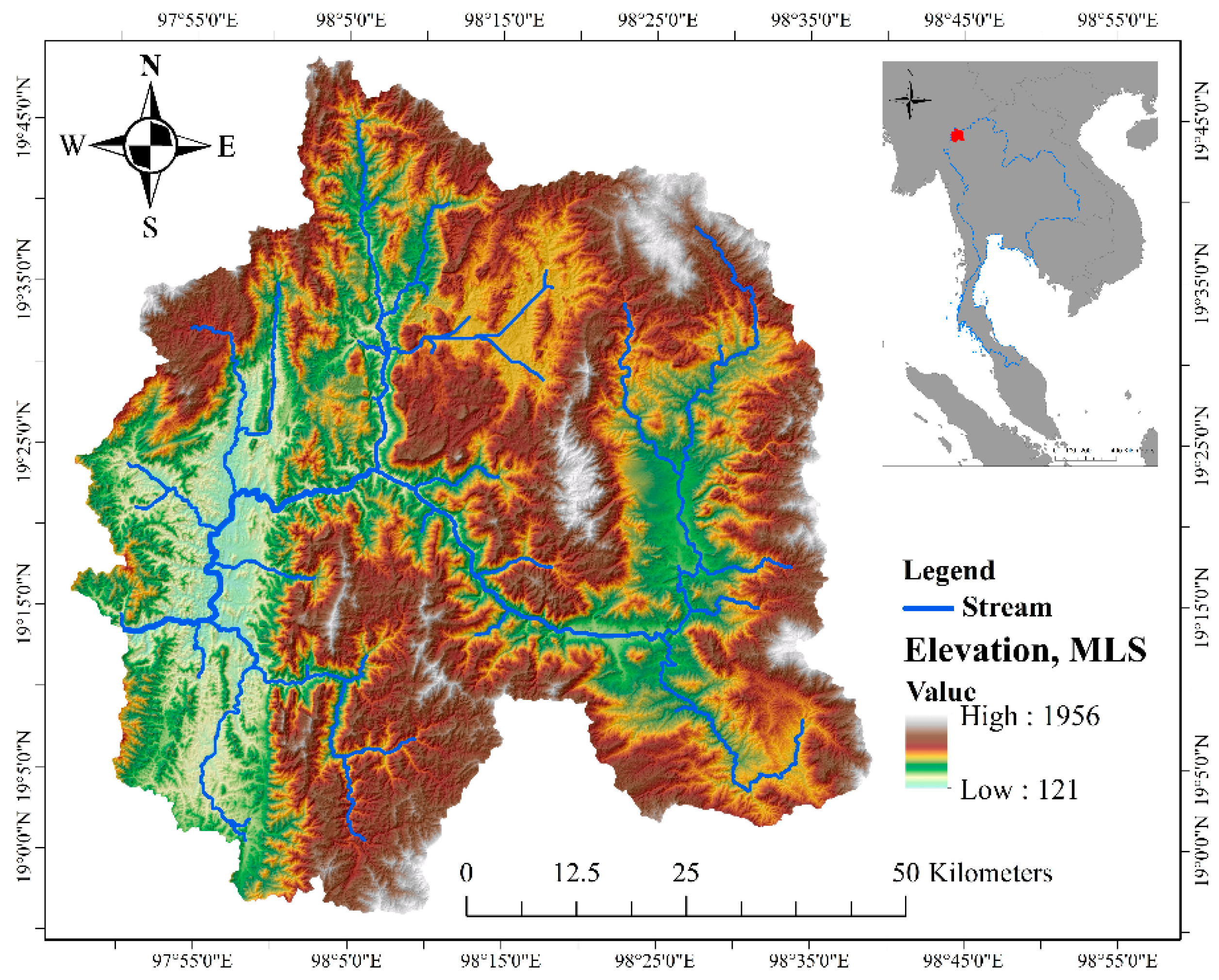
The Pai River basin is located in Mae Hong Son Province in northern Thailand and covers three districts (Mueang Mae Hong District, Pang Mapha District, and Pai District) in Mae Hong Son Province. The Pai River basin is a subwatershed of the Salween watershed, consisting of six river branches [27]. In Mae Hong Son Province, the watersheds are classified into classes A1 and 2, in which the main physical characteristic is a high slope gradient; moreover, the quality of these watersheds are suitable for the preservation of the upstream regions. The rainfall and its intensity in Mae Hong Son Province are influenced by the southwest monsoon in the rainy season (May to October). The average annual rainfall is approximately 1064.9 mm. Figure 1 presents the elevation and river network of the study area. Topographically, the study area is composed of complex high mountains and plains near rivers between valleys. The local people live in settled communities on the plains near rivers between valleys, and their paddy fields are located on the plains near rivers between valleys. Considering land use, forests and field crops compose the majority of the land use types in the study area.
3. Materials and Methods
3.1. Methods
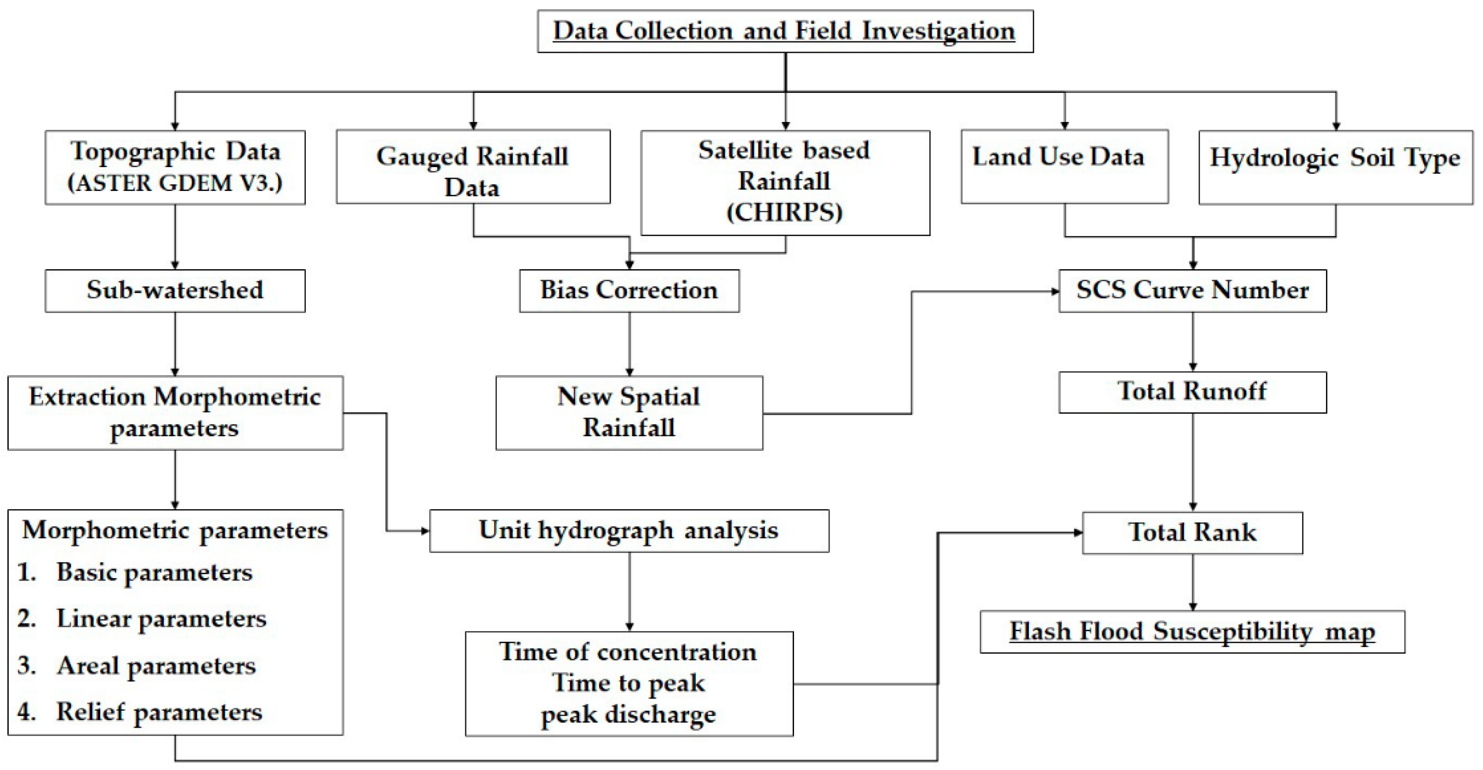
Figure 2 illustrates a summary of the methodology used in the study. The method used in the study can be divided into five parts and is explained in the following steps.
3.1.1. Quantitative Analysis of Morphometric Parameters
The first step is to extract the subwatersheds in the study area and quantitatively analyze the morphometric parameters of each subwatershed. The first part aims to use various mathematical procedures to determine the values of selected morphometric parameters. The subwatersheds and the 23 morphometric parameters are determined using ASTER GDEM Version 3. Before using ASTER GDEM Version 3 in the study, data preprocessing steps are applied to the DEM by removing the sinks by the filling method. Next, the subwatersheds are delineated by using a watershed function in which the flow direction based on the D8 flow method and the pour point grid are used to divide the water and delineate the catchment boundaries. The 23 morphometric parameters of the watershed can be categorized into four groups, basic, linear, areal, and relief features, as shown in Table 1.
3.1.2. Unit hydrograph Analysis
In the second step, we estimate the time of concentration (tc), time to peak (tp), and peak discharge (Qp) using Snyder’s synthetic unit hydrograph method. Snyder’s synthetic unit hydrograph method is based on relating morphometric parameters representing a drainage basin to describe the hydrological response structure of the basin, thus providing the travel time of effective rainfall flows along the stream network until the outlet of the watershed [37,38,39]. In Thailand, the equations for calculating the peak discharge in the Salween watershed can be expressed as follows:
where Qp is the peak discharge (cms), tp is the time to peak (h), Lc is the length of the stream from outlet to point opposite to centroid of watershed (km), L is the length of master stream from basin divide to outlet (km), and S is the average slope of the river.
The time of concentration equation is written as follows:
where H is ratio of the average slope of the river to the length of the master stream from the basin divide to the outlet.
3.1.3. Soil Conservation Service Curve Number Method
In the third step, we calculate the excess rainfall or total runoff by using the soil conservation service curve number method. The curve number method is widely used to estimate the depth of direct runoff from the rainfall depth because of its simplicity and applicability [40]. The curve number method uses the hydrologic soil type, land use type or surface condition, and depth of rainfall. The curve number method assumes that the ratio of the actual to maximum potential retention (S) of rainfall is expressed in the following equation:
where Qt is the watershed runoff, P is the rainfall depth, Ia is the initial abstraction, and S is the maximum potential retention. In general, the initial abstraction is 20% of the maximum potential retention [41].
Considering land use and hydrologic soil types, past research has shown that there are a variety of land use types and hydrologic soil types in the watershed. Hence, composite watershed CN values can be determined using the area-weighted averaging equation as follows:
Based on Equation (7), the area-weight averaging of CN values is linear; however, the CN equation does not vary linearly [42]. The runoff trends are nonlinear for smaller rainfall depths. Based on the recommendation of the USDA-NRCS in the Part 630 Hydrology National Engineering Handbook, the weighted watershed runoff method gives a more accurate result than the weighted-CN method, especially when a watershed has many complex land surface conditions and hydrologic soil types [43]. Hence, in this study, we adopted the weighted watershed runoff method for the total runoff calculation. The weighted watershed runoff is calculated using the following equation:
where Qt,comp is total watershed runoff, and Qt,i is total runoff from each individual area Ai with the different curve number values.
3.1.4. Local Calibration the Satellite Rainfall
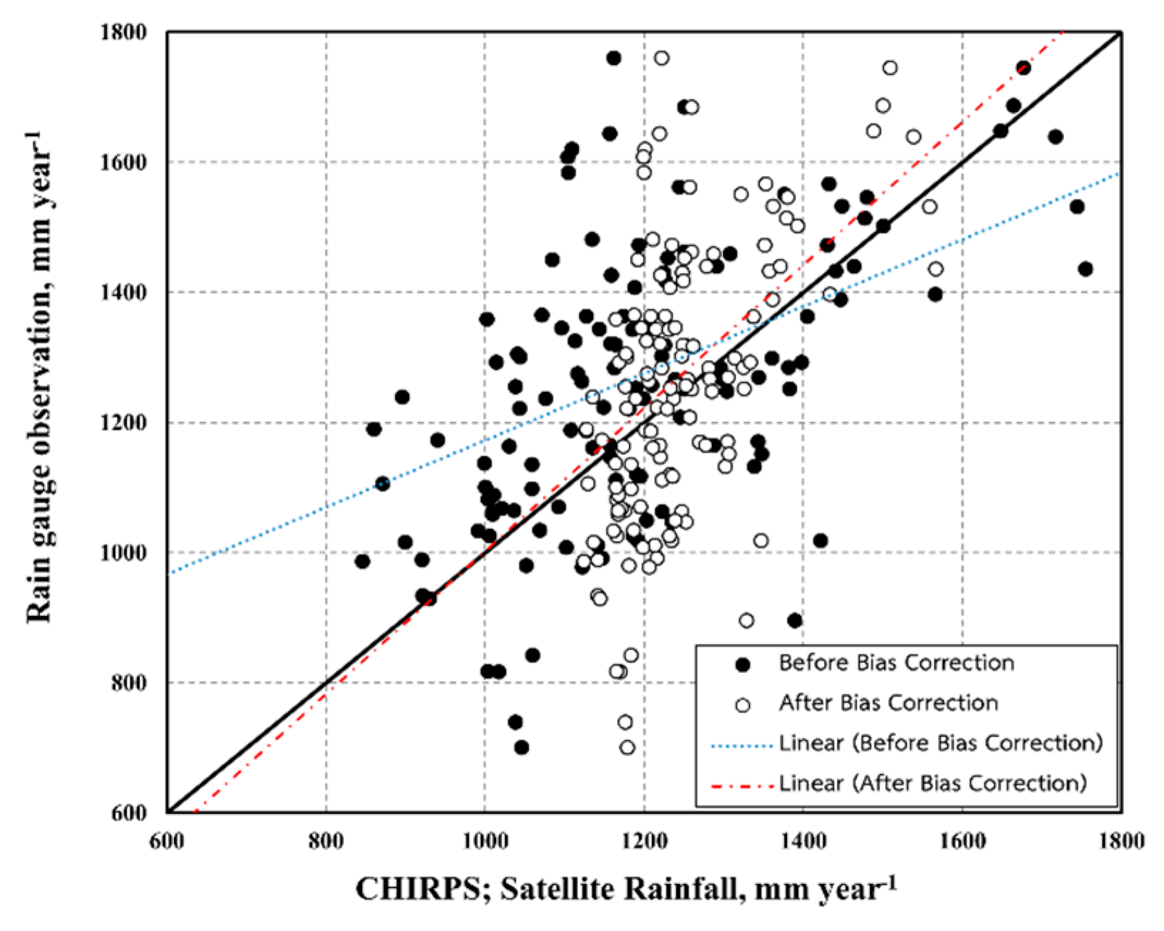
As mentioned previously, the rainfall depth is the key parameter for estimating the total watershed runoff. To adjust the bias of satellite rainfall, in this study, we adopted regression analysis to calibrate the satellite rainfall data with the locally gauged rainfall data. The empirical relationships between the satellite-derived and locally gauged rainfall data series can be derived from the linear regression equation covering the annual period from 1981 to 2010. In addition, rainfall data collected from 2011 to 2020 were used to validate the performance of the bias correction method. The root mean square error (RMSE) was used to measure the differences between satellite rainfall and locally gauged rainfall [44].
3.1.5. Ranking of All Parameters for the Categorized the Sub-Watershed
Finally, in the fifth step, we rank the standardized parameters for the categorized watersheds. Considering the first to fourth parts, the selected parameters in each subwatershed were calculated and expressed in different units, so they were normalized. Before the ranking and normalized processes, the selected parameters were separated into two groups. The group-I parameters were assumed to be positively correlated with flash flooding; in contrast, the group-II parameters were assumed to be negatively correlated with flash floods [45,46]. The equations used to obtain the normalized morphometric parameters can be expressed as follows:
where xmin is the minimum value of each morphometric parameter. xmax is the maximum value of each morphometric parameter.
3.2. Data
To achieve the objective of this study, the Advanced Spaceborne Thermal Emission and Reflection Radiometer (ASTER) Global Digital Elevation Model Version 3 (GDEM 003) or ASTER GDEM V3 was used to extract the morphometric parameters of the overall watershed and of each subwatershed. The ASTER GDEM V3 is the newest version of the ASTER GDEM and was released in 2019; this product was developed by the Ministry of Economy, Trade, and Industry (METI) of Japan and the United States National Aeronautics and Space Administration (NASA). The grid resolution of ASTER GDEM V3 is 30 m.
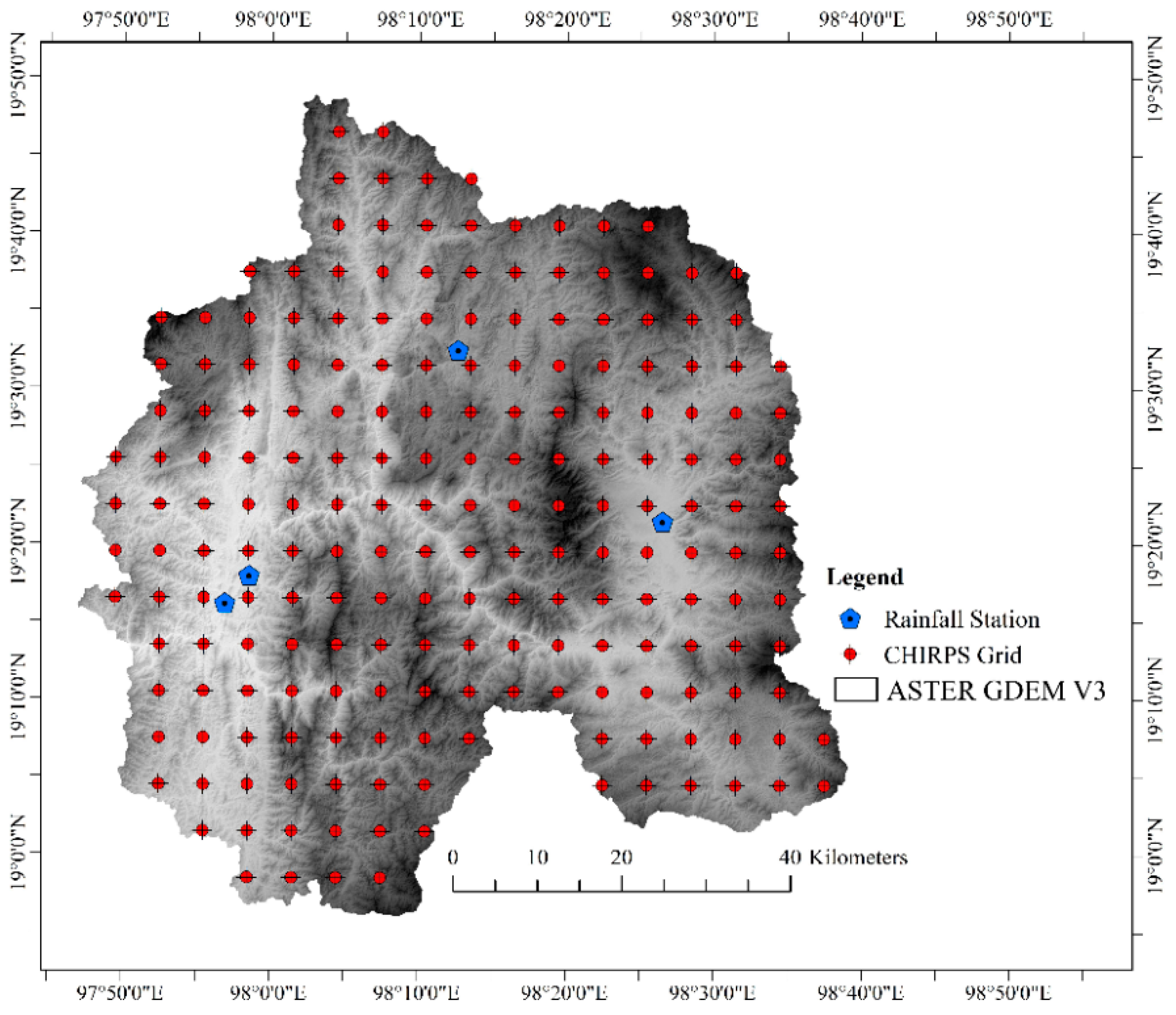
For rainfall data, two datasets are applied: gauged rainfall data and satellite-based precipitation data. The gauged rainfall data used in this study were measured and operated by the Thai Meteorological Department (TMD) and Royal Irrigation Department (RID). Annual rainfall data recorded from 1981 to 2020 were used in this study The satellite-based precipitation data used in the study are derived from the CHIRPS product. CHIRPS was developed by the Climate Hazards Center at the University of California, Santa Barbara. CHIRPS estimates precipitation data globally at a 0.05-degree resolution from 1981 to near-present spanning 50 °S–50 °N. In this work, precipitation was estimated based on the infrared cold cloud duration; moreover, the data incorporated with gauged rainfall data are the GHCN monthly, GHCN daily, Global Summary of the Day (GSOD), GTS, and Southern African Science Service Centre for Climate Change and Adaptive Land Management data [19]. Figure 3 illustrates the ASTER GDEM V3, the locations of the rain gauges, and the CHIRPS grid considered in this study.
To calculate annual runoff, the land use types and hydrologic soil types are the key parameters for determining the curve number value in the soil conservation service curve number (SCS-CN) model. The land use data considered in this study were generated by the Land Development Department of Thailand, Ministry of Agriculture and Cooperatives. The hydrological soil type data were developed by the NASA Carbon Cycle Science program based on the Food and Agriculture Organization soilGrids250m system to support USDA-based curve-number runoff modeling at regional and continental scales [26]. The hydrologic soil type data are divided into four soil type groups: A (low runoff potential), B (moderately low runoff potential), C (moderately high runoff potential), and D (high runoff potential).
4. Results and Discussion
4.1. Sub-Watersheds and Their Morphometric Parameters
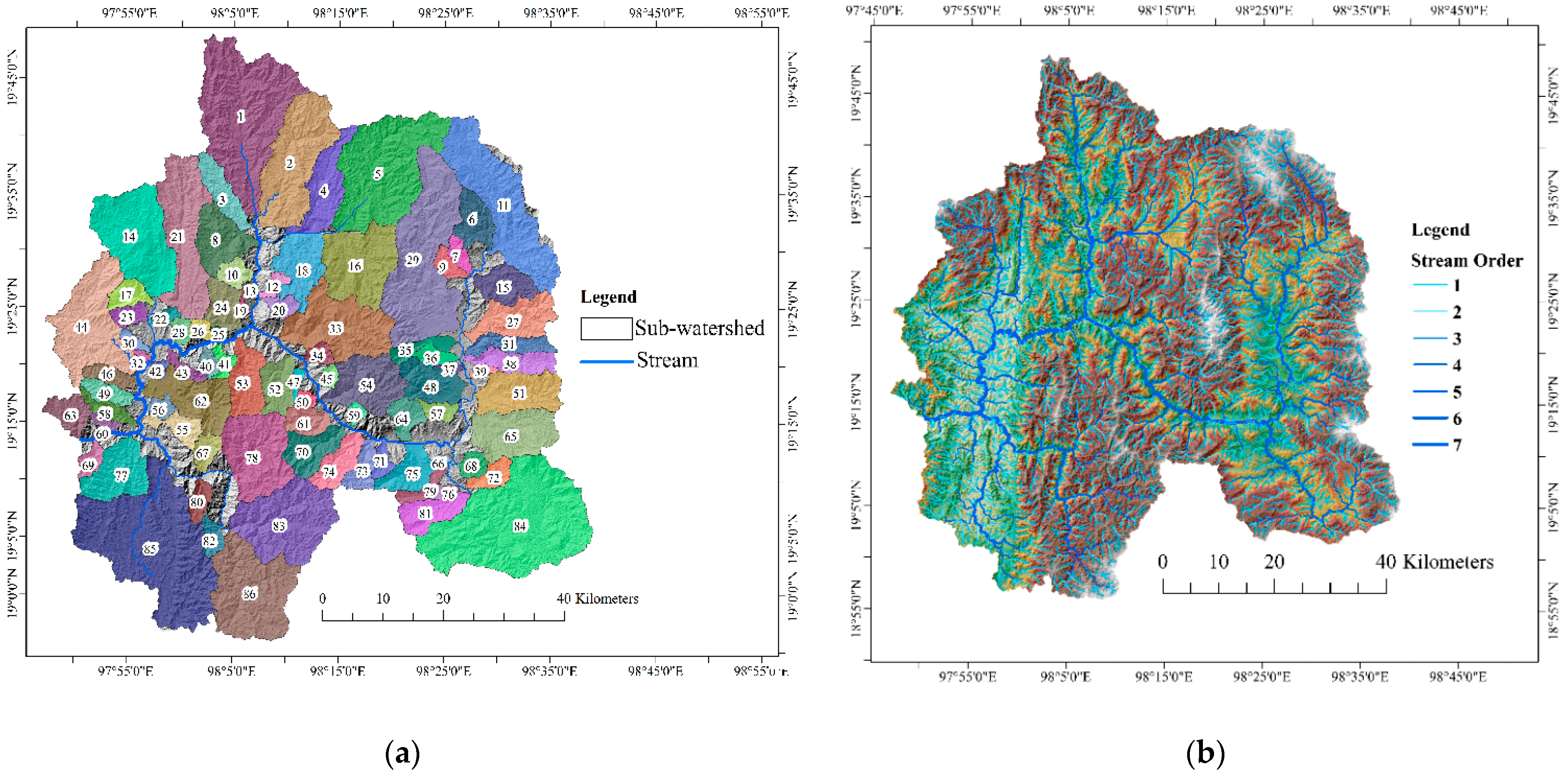
According to the subwatershed extraction results derived based on the first step of the methods described above, the study area was divided into 86 subwatersheds. In addition, the extraction of stream order is a key step for calculating the morphometric parameters of watersheds. The Strahler method was used to extract the stream order in this study. The stream order increases when streams of the same order merge. Hence, the stream network in the study consists of first, second, third, fourth, fifth, sixth, and seventh stream-order channels. Figure 4 illustrates the subwatershed and stream order network considered in this study. According to the analysis, the largest basin is subwatershed no. 85; the area of subwatershed no. 85 is approximately 353 km2. Moreover, this subwatershed has the longest total stream length in the study area, at approximately 376 km.
4.1.1. Linear Features Group
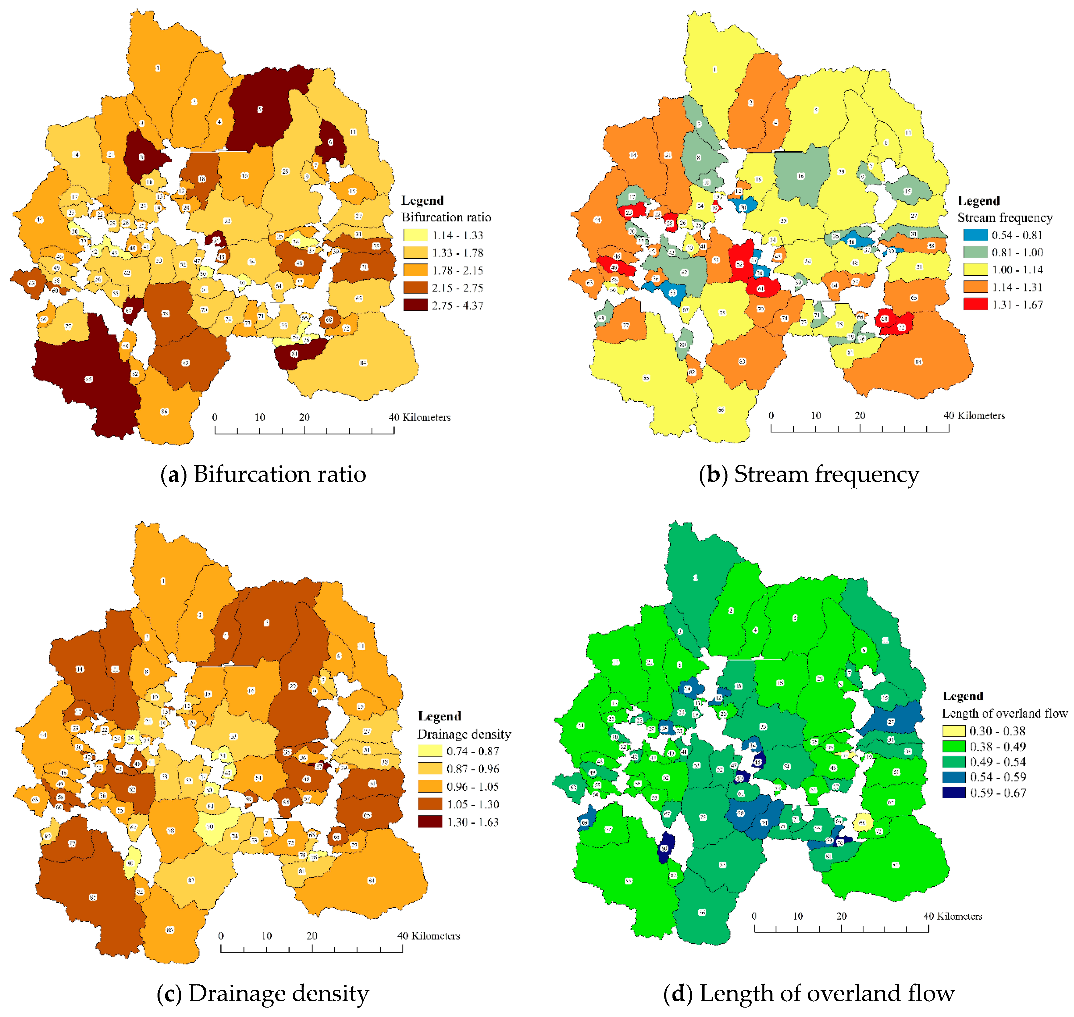
The bifurcation ratio is defined as the ratio of the total stream number of one order to the total stream number of the next-highest order [33]. The bifurcation ratio represents the geological, lithological, and tectonic characteristics of a drainage basin [47]. A high bifurcation ratio indicates that the runoff-producing potential of the drainage basin is high [48]. If a drainage basin has lower bifurcation ratio values, this indicates plain terrain [49]. In this study, the values of the bifurcation ratio vary from 1.14 (subwatershed no. 79) to 4.37 (subwatershed no. 5).
The stream frequency is the ratio of the total stream number to area [29]. Lower stream frequency values indicate that the surface runoff is slower; in contrast, high stream frequency values imply rapid surface runoff [13,48]. The stream frequency values derived in the study are between 0.54 (subwatershed no. 39) and 1.67 (subwatershed no. 19).
The drainage density is calculated as the total stream length divided by the basin area. A high drainage density value reflects a high runoff volume and a rapid response with respect to rainfall and the rapid flood peak [47]. In this analysis, the highest obtained drainage density value is 1.63 (subwatershed no. 37), and the lowest drainage density value is 0.74 (subwatershed no. 50).
The length of overland flow is the length of water flowing over the ground surface before it becomes concentrated in stream channels. The length of overland flow is approximately equal to half the reciprocal of the drainage density [29]. The length of overland flow values in the study vary from 0.31 (subwatershed no. 37) to 0.67 (subwatershed no. 50).
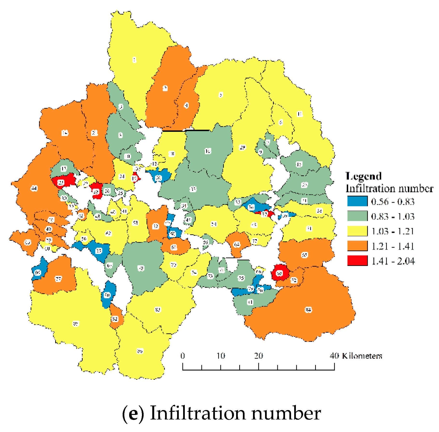
The infiltration number is a morphometric parameter used to understand the infiltration potential of a watershed; a higher infiltration number value is expected to result in higher runoff and lower infiltration [49]. The infiltration number is defined as a function of the drainage density and stream frequency. The infiltration number values in the studied subwatersheds vary from 0.56 (subwatershed no. 39) to 2.04 (subwatershed no. 68). Figure 5 illustrates a group of linear feature parameters consisting of the bifurcation ratio, stream frequency, drainage density, length of overland flow, and infiltration number.
4.1.2. Areal Features Group
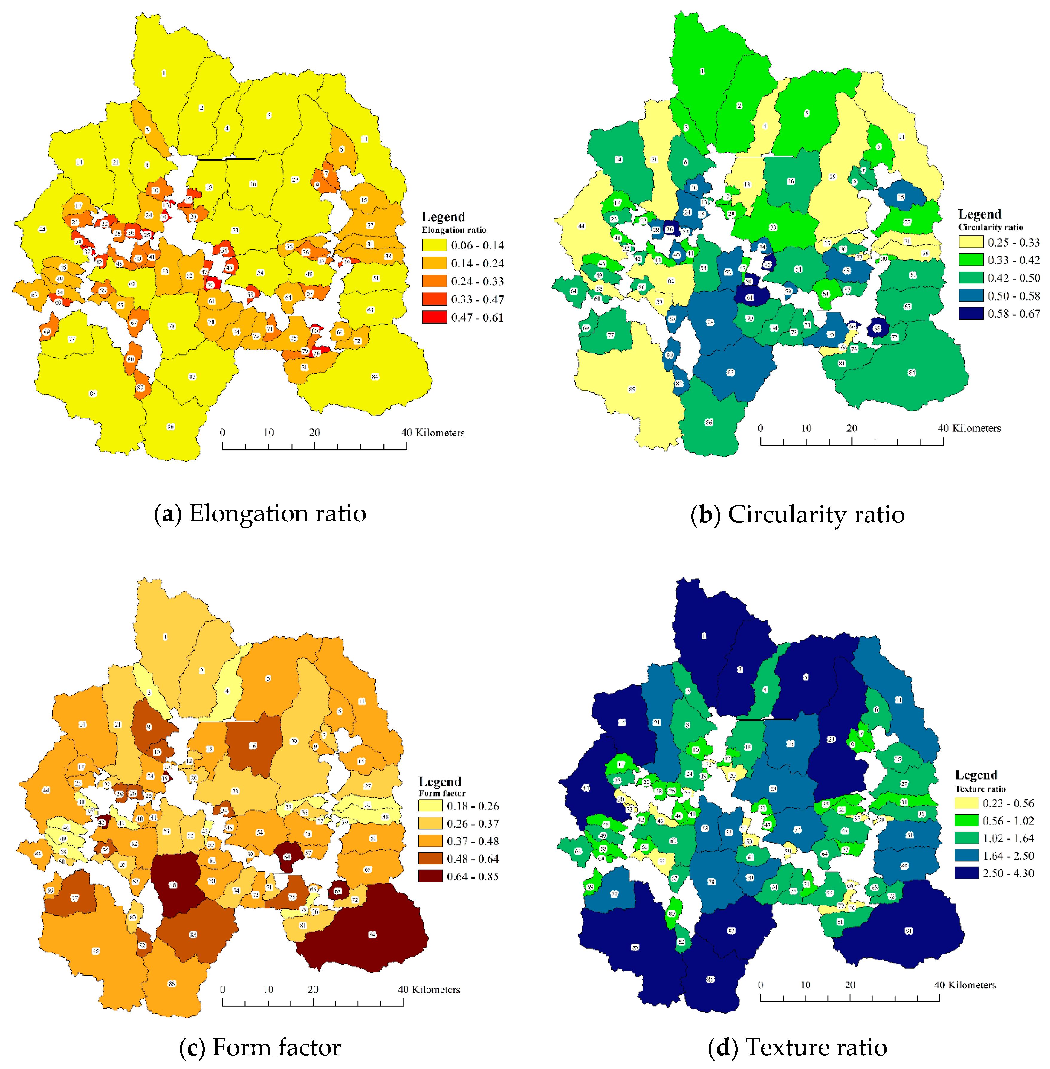
The elongation ratio is a morphometric parameter representing the shape of the watershed. The elongation ratio can be calculated by obtaining the ratio of a circle diameter with the same area of the watershed to the maximum basin length [50]. Typically, the elongation ratio values range between 0 and 1. If the elongation ratio approaches 1, the shape of the watershed is near-circular. The values of the elongation ratio can be classified into four groups: circular (>0.9), oval (0.9–0.8), less elongated (0.8–0.7), and elongated (<0.7) [48]. A circular watershed shape generates a high discharge peak. In this study, the elongation ratios range from 0.06 (subwatershed no. 85) to 0.61 (subwatershed no. 13), indicating that the subwatersheds have less elongated to elongated shapes.
The circularity ratio is defined as ratio between the basin area and the area of a circle with a circumference equal to the perimeter of the basin [51]. When the circularity ratio approaches 0, the shape of the basin is elongated. In contrast, higher circularity ratio values indicate that the shape of the basin is more circular. The circularity ratio values derived in the study vary from 0.25 (subwatershed no. 4) to 0.67 (subwatershed no. 26).
The form factor is defined as the basin area divided by the square of the basin length. Typically, form factor values range from 0.1 to 0.8, and smaller form factor values indicate that the shape of the basin is more elongated [51]. The value of the form factor can be interpreted to indicate that shorter-duration high peak flows occur in basins alongside relatively high form factor values. According to the analysis, the form factor values derived in the study range from 0.18 (subwatershed no. 58) to 0.85 (subwatershed no. 78).
The texture ratio is the ratio of the total stream number to the basin perimeter. The texture ratio can be divided as follows: coarse texture (<4 per km), intermediate texture (4–10 per km), fine texture (10–15 per km), and very fine texture (>15 per km) [52]. Drainage basins with coarse textures exhibit trends of high basin lag times [52]. The texture ratios derived herein range from 0.23 (subwatershed no. 39) to 4.30 (subwatershed no. 84).
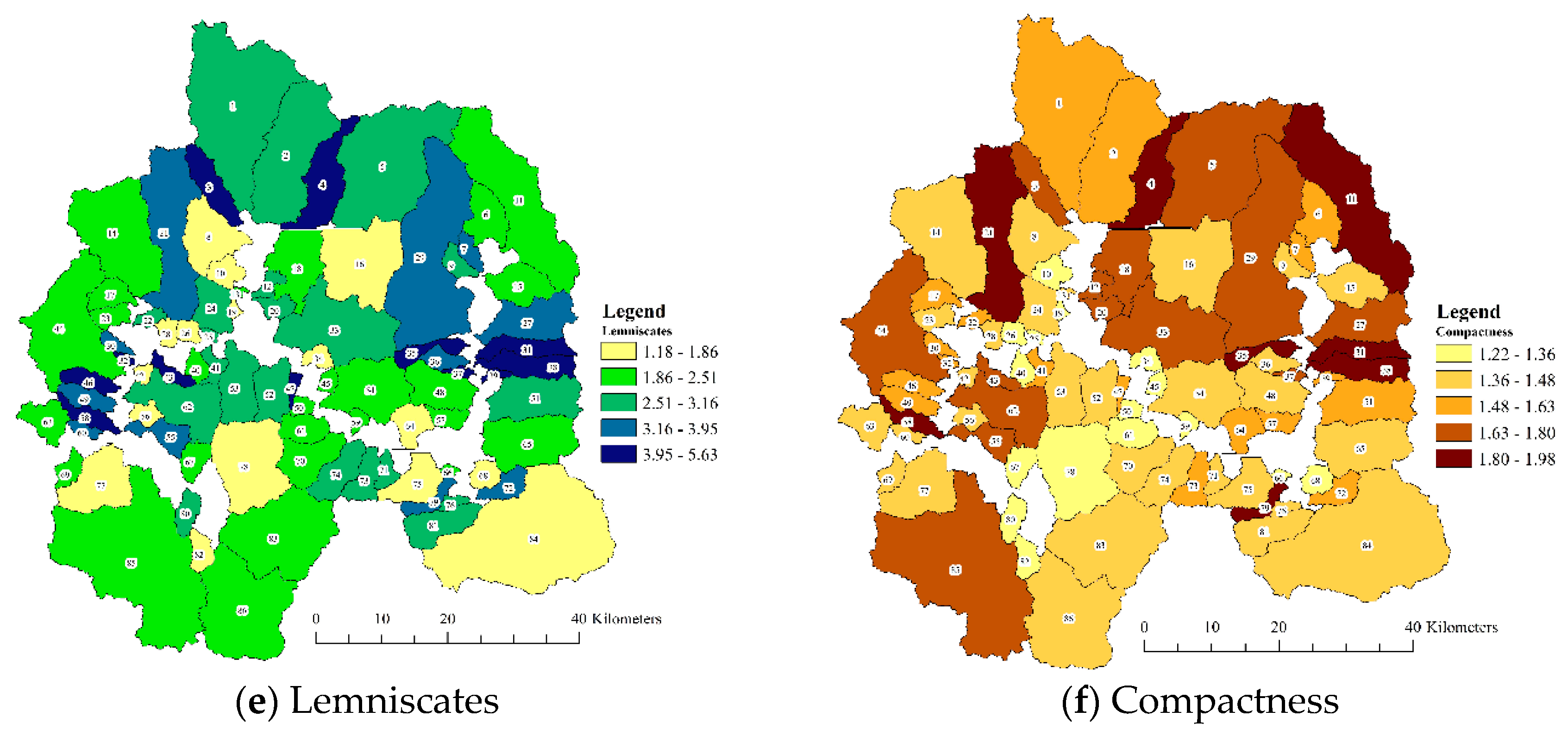
The lemniscates approximate the actual watershed shape better than the circularity ratio [36]. Lemniscate ratio values less than 0.5 imply that the basin shape is most likely circular, and circular basins tend to have shorter concentration times when compared to fully elongated basins with lemniscate ratios greater than 2.5 [50]. In this study, the lemniscate values vary from 1.18 (subwatershed no. 78) to 5.63 (subwatershed no. 58).
The compactness is defined as the ratio of the perimeter of a drainage basin to that of a circle of equal area [34]. Flooding risks form mostly in basins with compactness values greater than 1 [50]. According to the analysis, in this study, the compactness values range from 1.22 (subwatershed no. 26) to 1.98 (subwatershed no. 4). Figure 6 illustrates that the group of areal feature parameters consists of the elongation ratio, circularity ratio, form factor, texture ratio, lemniscates, and compactness.
4.1.3. Relief Features Group
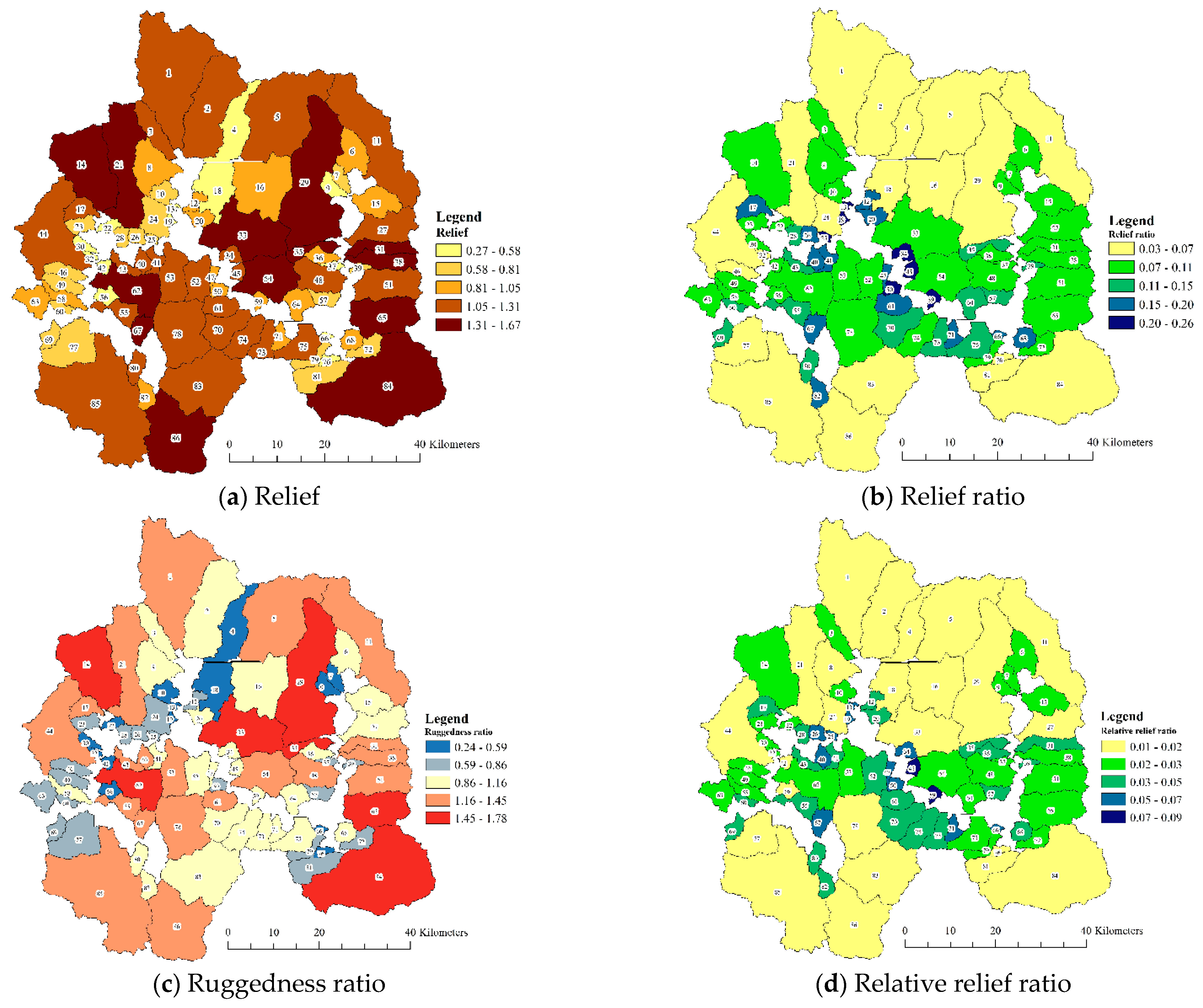
Relief is a significant morphometric parameter and is widely used to quantitatively assess hydrological models. Relief is useful for explaining the gradients of drainage basins or the sediment transport process [13]. Relief is defined as the difference between the highest elevation and lowest elevation of a basin. In this study, the relief values range from 1.67 km (subwatershed no. 14) to 0.27 km (subwatershed no. 32).
The relief ratio is a topographic indicator used to assess the entire slope processes of a drainage basin along with the water flow dynamic intensity [50]. The relief ratio is calculated as the ratio of the overall terrain range of the drainage basin to the length of the drainage basin. High relief ratio values indicate an intense flow capability with accelerated morphodynamic processes on steep slope basins related to erosion and sediment yield [46]. In the current study, the relief ratio values range between 0.027 (subwatershed no. 4) and 0.26 (subwatershed no. 45).
The ruggedness ratio is calculated by multiplying the relief value by the drainage density. High ruggedness ratio values occur in steeply sloped basins that respond to rapid peak flow and flash floods [13]. Generally, a ruggedness ratio less than 1 implies flat topography, values between 1 and 2 indicate undulating topography, and values above 2 indicate badland topography [45]. The ruggedness ratio value in the study ranges from 0.24 (subwatershed no. 76) to 1.77 (subwatershed no. 14).
The relative relief ratio is defined as the basin relief divided by the basin perimeter. The relative relief ratio is often utilized to present a relief map of drainage basin dimensions without considering sea level [48]. The values of the relative relief ratio obtained in this study are between 0.008 (subwatershed no. 4) and 0.08 (subwatershed no. 45). Figure 7 illustrates that the group of relief feature parameters comprises relief, the relief ratio, the ruggedness ratio, and the relative relief ratio.
4.2. Calibration of Rainfall
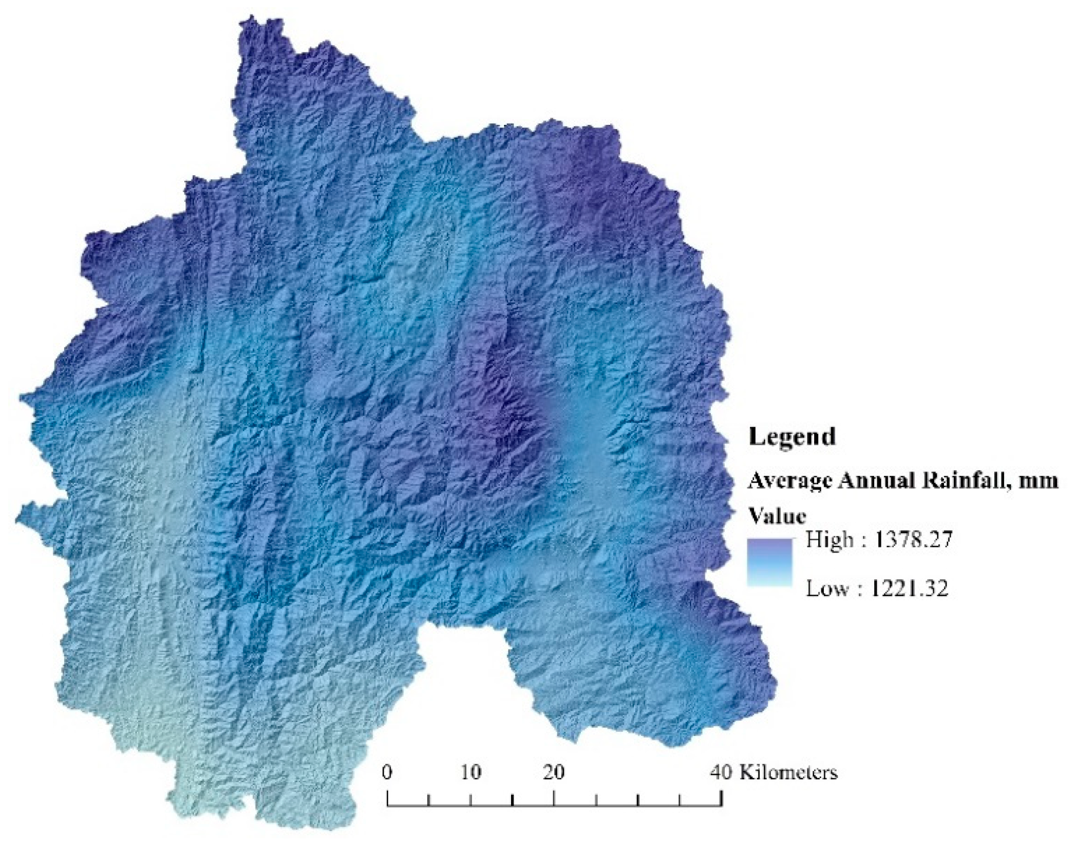
Figure 8 illustrates plots of annual rainfall derived using the gauged rainfall data and CHIRPS data (satellite-based rainfall) before and after the bias-correction process. The RMSE is used to indicate the differences between the satellite-derived rainfall and locally gauged rainfall before and after the bias-correction process. As mentioned in Section 3.1.4, a linear regression equation was built and applied to calibrate the CHIRPS data. The RMSE of the uncorrected annual satellite-based rainfall data was approximately 254 mm. The RMSE of the corrected annual satellite-based rainfall data was approximately 224 mm. A comparison between the RMSE values before and after the bias-correction step was applied showed that the RMSE value was reduced by approximately 30 mm after the CHIRPS data passed the bias-correction process using the gauged rainfall data. Considering the plot of annual rainfall between the gauged rainfall data and the CHIRPS data, the points of corrected annual satellite-based rainfall data are more aligned and less scattered compared to the uncorrected annual satellite-based rainfall. After the bias-correction process, new spatial rainfall data were generated using the linear regression equation and the CHIRPS rainfall data from 1981 to 2020. Then, the spatial rainfall data were averaged to calculate the mean annual rainfall depth. Figure 9 illustrates the spatial distribution of the mean annual rainfall depth in the study area. Considering the spatial distribution of the mean annual rainfall data, high mean annual rainfall depths occurred in the mountainous areas in the upper and middle parts of the study area.
4.3. Unit Hydrograph Analysis
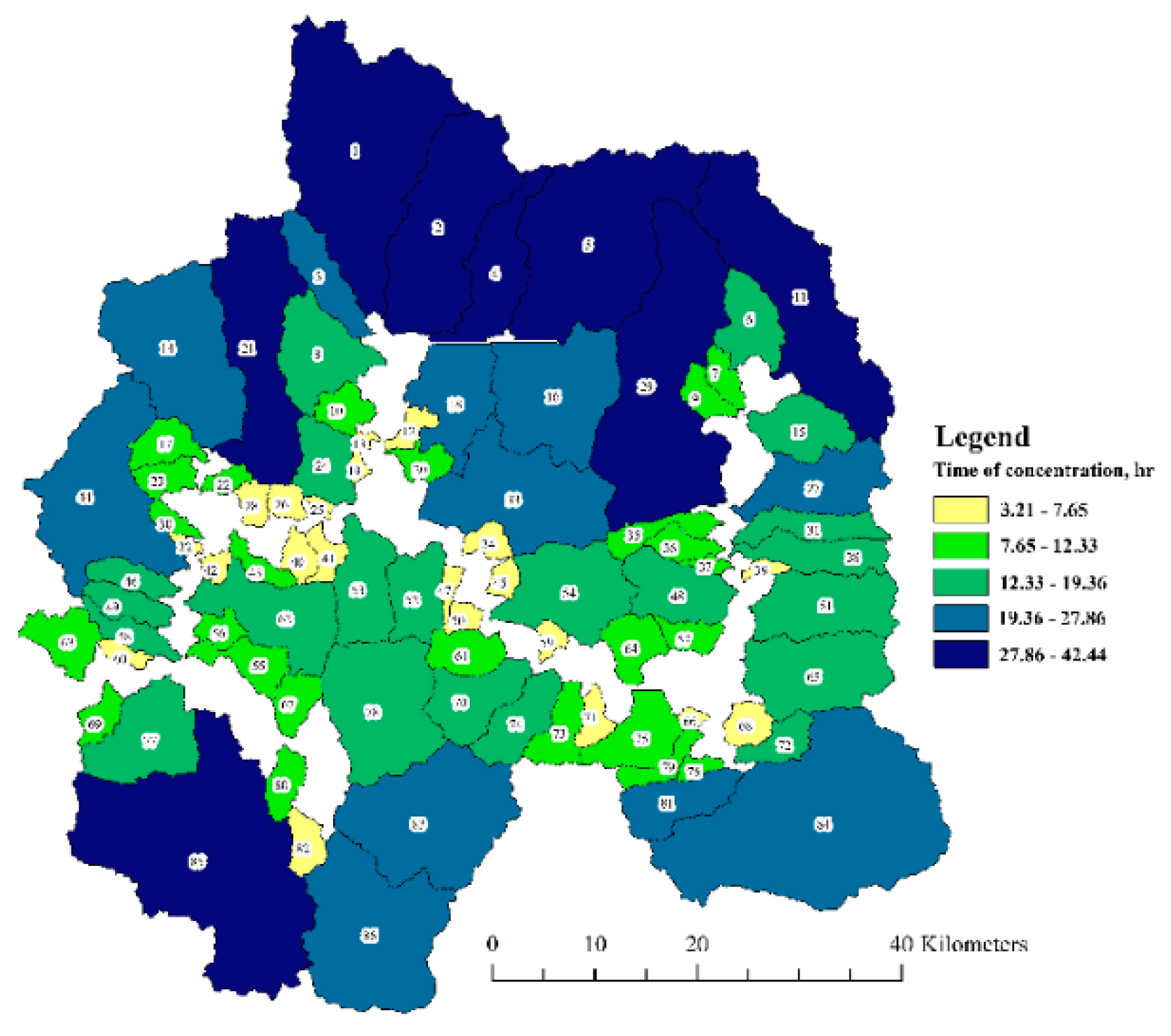
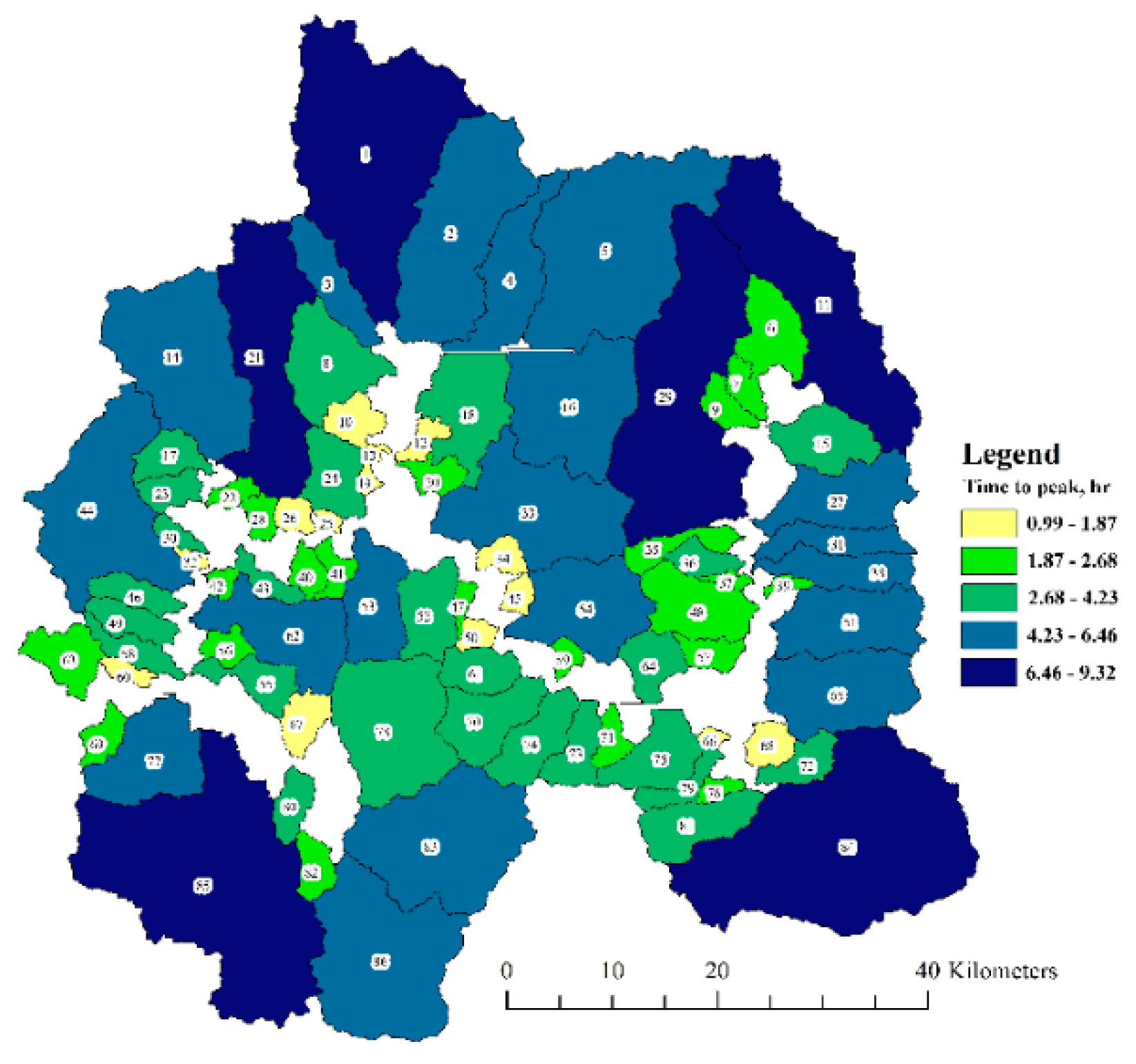
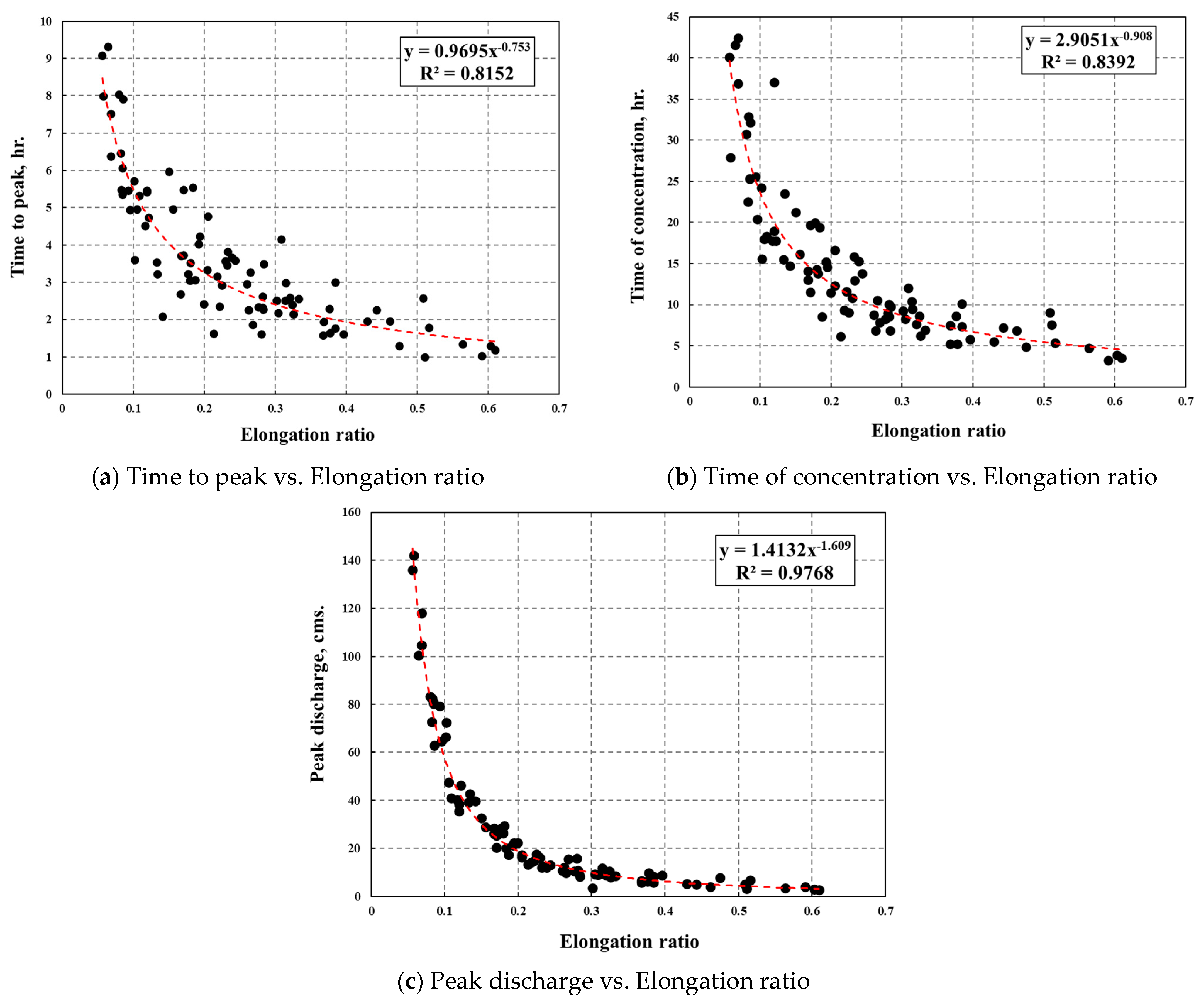
The time of concentration, peak discharge, and time to peak are important parameters; in this work, these parameters were calculated using Snyder’s synthetic unit hydrograph method. Figure 10 illustrates the time of concentration of the subwatersheds considered in the study. Figure 11 illustrates the peak discharge of the subwatersheds. Figure 12 illustrates the time to peak of the subwatersheds. The times of concentration in the study range from 42.4 h (subwatershed no. 1) to 3.2 h (subwatershed no. 19). The times to peak range from 9.32 h (subwatershed no. 29) to 0.987 h (subwatershed no. 32). The peak discharges range from 141.96 mm (subwatershed no. 84) to 2.66 mm (subwatershed no. 13). Considering the relation between the time of concentration and morphometric parameters of the watershed, the time of concentration was high when the elongation ratio was low. The watersheds with low elongation ratio values indicate having quite elongated drainage basin shapes, so the surface runoff time interval is longer than that in basins with circular shapes. The relation between the time of concentration and elongation ratio can be generated using the power equation shown in Figure 13a. In addition, the time to peak also has the same relation with the elongation ratio; the relation between the time to peak and elongation ratio can be generated by obtaining a trendline using the power equation, as shown in Figure 13b. Moreover, in this study, it was found that the peak discharge also has a strong correlation with the elongation ratio, as shown in Figure 13c.
4.4. Total Watershed Runoff
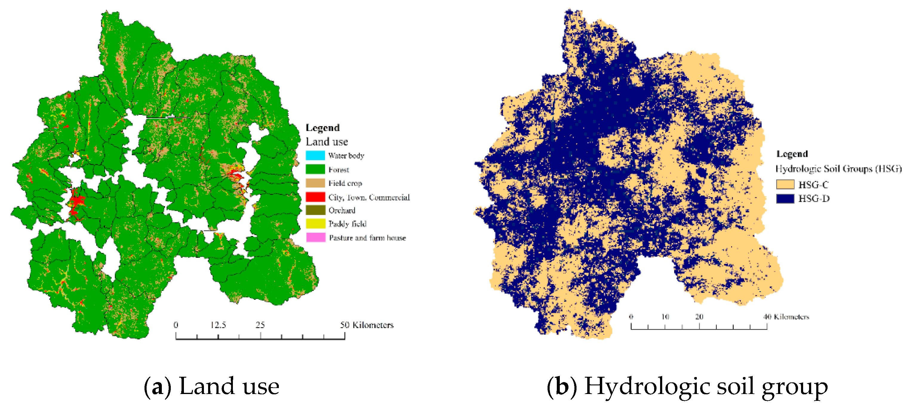
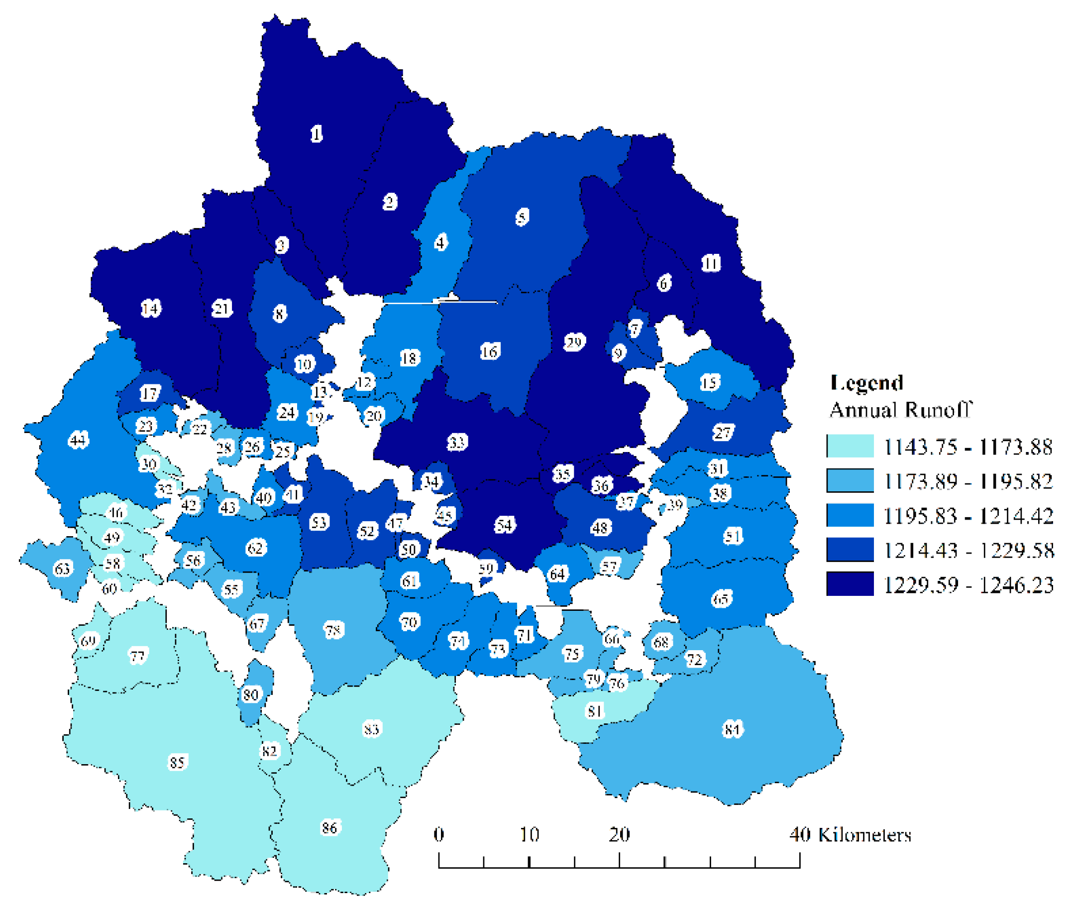
The surface runoff characteristics of watersheds play an important role in flash flood occurrence. The surface runoff volumes are dependent on several factors, such as the land use or land cover type, soil type, or rainfall characteristics. Based on the soil conservation service curve number method, the CN values depend on the soil and land use types in each area. The dominant land use type in the study area is forest; moreover, there are scattered field crop areas in many areas. Paddy fields are mostly located near rivers, and villages are located around these paddy fields. Regarding the hydrologic soil type, two hydrologic soil groups are identified in the study area: group C (moderately high runoff potential in which the soil components are <50% sand and 20–40% clay) and group D (high runoff potential in which the soil components are <50% sand and >40% clay). Figure 14 illustrates the land use and hydrologic soil groups in the study area. According to the analysis results, the highest runoff is approximately 1246 mm (subwatershed no. 11), and the lowest runoff is approximately 1143 mm (subwatershed no. 85). One of the factors influencing the amount of runoff is rainfall because the hydrologic soil groups and land use types are not significantly different across the study area. Hence, considering the mean annual rainfall depth shown in Figure 9, subwatershed no. 11 is an area where the mean annual rainfall depth is high; in contrast, subwatershed no. 15 corresponds to low mean annual rainfall depths. Figure 15 illustrates the annual runoff in each subwatershed.
4.5. Flash Flood Susceptibility Mapping
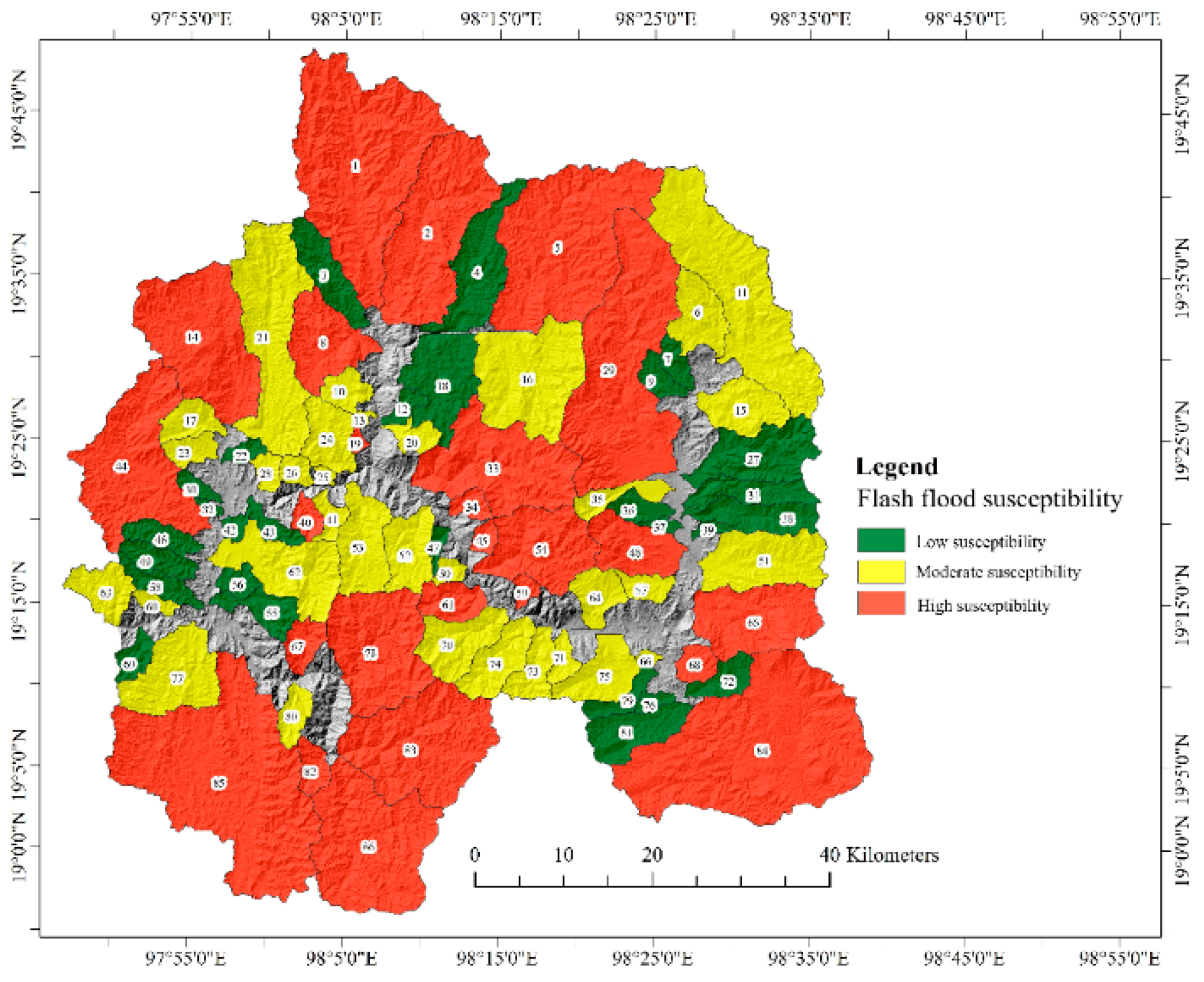
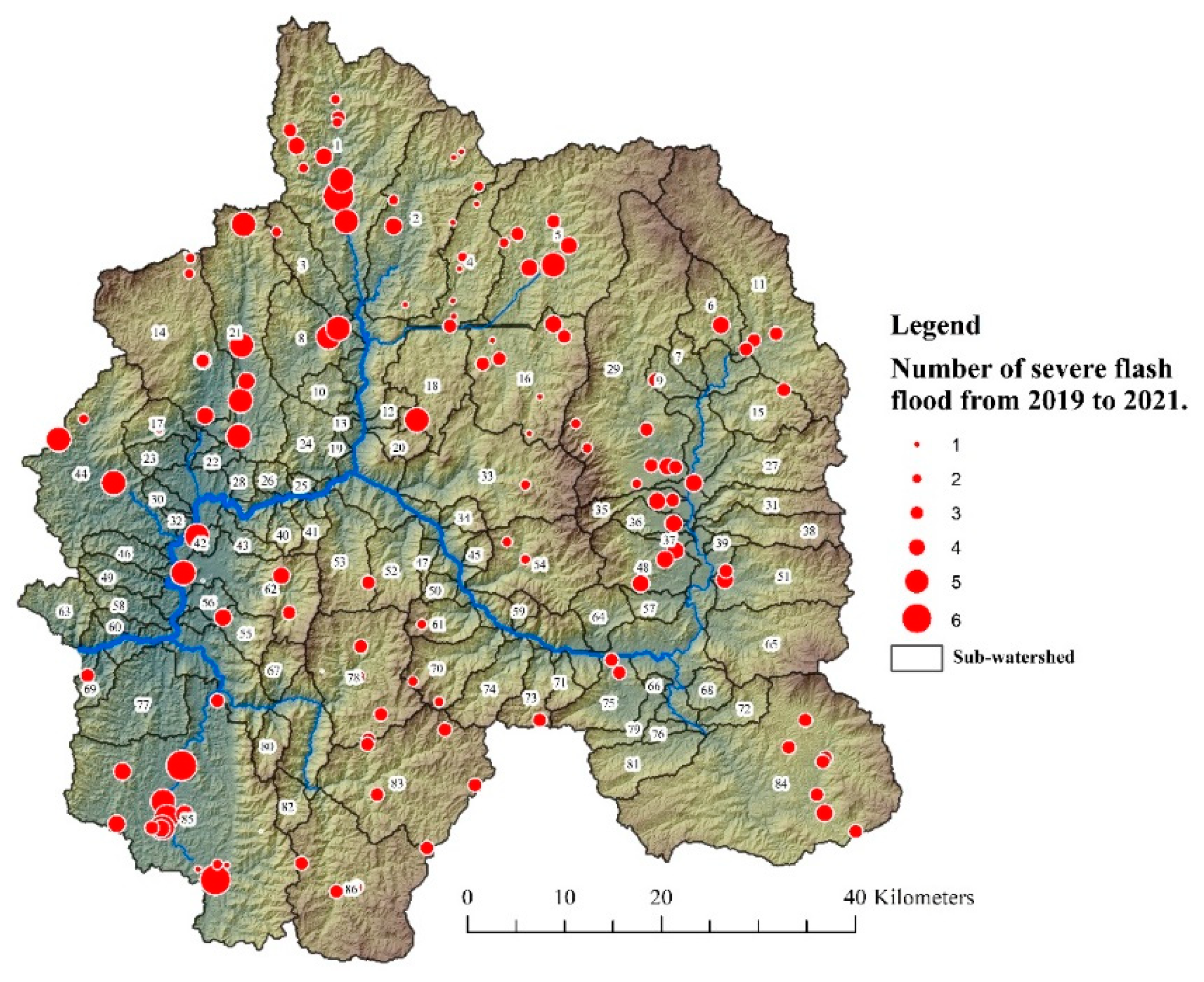
The degree of flash flood susceptibility is quantitatively determined by ranking the subwatersheds using 21 morphometric watershed parameters, the time of concentration, the time to peak, the peak discharge, and the annual runoff of each subwatershed. The aggregated scores of the subwatersheds in the study area rank from 88.4 (subwatershed no. 68) to 55.5 (subwatershed no. 4). The flash flood susceptibility level was classified into three classes, namely, high, moderate, and low susceptibility. The high-flash-flood-susceptibility level consists of 25 subwatersheds. For the moderate flash flood susceptibility level, there are 33 subwatersheds. There are 28 subwatersheds in the low-flash-flood-susceptibility level. To validate the results of the study, the villages affected by flash floods from 2019 to 2021 and the number of flash flood events were recorded from the declaration of disaster-affected areas of the Department of Disaster Prevention and Mitigation (DDPM) of Thailand. Figure 16 illustrates the flash flood susceptibility map of the Pai River Basin, Mae Hong Son, Thailand. Figure 17 illustrates the number of severe flash flood events that occurred in the villages from 2019 to 2021. Comparing the flash flood susceptibility map and the record of flash flood events, the results of the study correspond with the record of flash flood events.
Given their mutually high susceptibility to flash flooding, there are many similarities in the morphometric characteristics of the subwatersheds in this study; namely, highly susceptible subwatersheds also have high relief, relief ratio, ruggedness, stream frequency, texture ratio, annual runoff, and peak discharge values and low compactness and elongation ratio values. In subwatersheds with low susceptibility to flash flooding, some similarities can be found in their morphometric characteristics, namely, low relief, relief ratio, basin slope, form factor, stream number, and relative relief ratio values. The inclusion of a geomorphological aspect improves the understanding of the physical characteristics that control the landforms of these basins. Additionally, it gives an interesting perspective for the flash floods risk zones determination [53].
5. Conclusions
Flash floods are serious natural hazards. Flash flood-prone areas are mountainous areas featuring steep terrain or complex orography. High-intensity localized rainfall is the main factor initiating flash flood occurrence. In this study, we used the morphometric parameters of a watershed to combine the characteristic features of hydrographs with the annual runoff characteristics to assess the susceptibility level of flash floods in the Pai River Basin, Mae Hong Son, Thailand. Accordingly, a combination of morphometric watershed characteristics and hydrological models can assess flash flood-susceptible areas. The results are in agreement with historical flash flood events. This technique is a useful tool for identifying areas susceptible to flash floods, especially areas in ungauged watersheds. In addition, this study can summarize the morphometric characteristics of drainage basins that are susceptible to flash flooding as follows: these basins have high relief, relief ratio, ruggedness, stream frequency, texture ratio, annual runoff, and peak discharge values and low compactness and elongation ratio values.
Funding
This research was funded by the Faculty of Social Sciences, Kasetsart University, Thailand.
Institutional Review Board Statement
The study was conducted in accordance with the Declaration of Helsinki, The Belmont Report, CIOMS Guideline, International Conference on Harmonization in Good Clinical Practice (ICH-GCP) and 45CFR 46.101(b) and approved by the Kasetsart University Research Ethics Committee (COE65/029 and 11 February 2022).
Informed Consent Statement
Not applicable.
Data Availability Statement
ASTER GDEM Version 3 at https://asterweb.jpl.nasa.gov/gdem.asp (accessed on 2 October 2022), CHIRPS at https://www.chc.ucsb.edu/data/chirps (accessed on 2 October 2022).
Acknowledgments
This research was supported by the Faculty of Social Sciences, Kasetsart University. The authors gratefully acknowledge the rainfall data of the Thai Meteorological Department (TMD) and the land use data of the Land Development Department of Thailand.
Conflicts of Interest
The authors declare no conflicts of interest.
References
- Chantip, S.; Marjang, N.; Pongput, K. Development of dynamic flash flood hazard index (DFFHI) in Wang river basin, Thailand. In Proceedings of the 22nd IAHR-APD Congress 2020, Sapporo, Japan, 15–16 September 2020. [Google Scholar]
- Quesada-Román, A. Flood risk index development at the municipal level in Costa Rica: A methodological framework. Environ. Sci. Policy 2022, 133, 98–106. [Google Scholar] [CrossRef]
- Bhaskar, N.R.; French, M.N.; Kyiamah, G.K. Characterization of flash flood in eastern Kentucky. J. Hydrol. Eng. 2000, 5, 3237–3331. [Google Scholar] [CrossRef]
- Wu, J.; Liu, H.; Wei, G.; Fu, G.; Markus, M.; Ye, L.; Zhang, C.; Zhou, H. Flash flood peak estimation in small mountainous catchment based on distributed geomorphological unit hydrographs using Fuzzy C-means Clustering. J. Hydrol. Eng. 2020, 25, 04020051. [Google Scholar] [CrossRef]
- Kim, B.-S.; Kim, H.-S. Evaluation of flash flood severity in Korea using the modified flash flood index (MFFI). J. Flood Risk Manag. 2014, 7, 344–356. [Google Scholar] [CrossRef]
- Koutroulis, A.G.; Tsanis, I.K. A method for estimating flash flood peak discharge in a poorly gauged basin: Case study for the 13-14 January 1994 flood, Giofiros basin, Crete, Greece. J. Hydrol. 2010, 385, 150–164. [Google Scholar] [CrossRef]
- Quesada-Román, A.; Ballesteros-Cánovas, J.A.; Granados-Balaños, S.; Birkel, C.; Stoffel, M. Improving regional flood risk assessment using flood frequency and dendrogeomorphic analyses in mountain catchments impacts by tropical cyclones. Geomorphology 2022, 396, 108000. [Google Scholar] [CrossRef]
- Ahn, K.-H.; Merwade, V. Role of watershed geomorphic characteristics on flooding in Indiana, United States. J. Hydrol. Eng. 2016, 21, 05015021. [Google Scholar] [CrossRef]
- Kocsis, I.; Bilașco, Ș.; Irimuș, I.-A.; Dohotar, V.; Rusu, R.; Roșca, S. Flash flood vulnerability mapping based on FFPI using gis spatial analysis case study: Valea Rea catchment area, Romania. Sensors 2022, 22, 3573. [Google Scholar] [CrossRef]
- Shehata, M.; Mizunaga, H. Flash flood risk assessment for Kyushu Island, Japan. Environ. Earth Sci. 2018, 77, 76. [Google Scholar] [CrossRef]
- Ikirri, M.; Faik, F.; Echogadali, F.Z.; Antunes, I.M.H.R.; Abioui, M.; Abdelrahman, K.; Fnais, M.S.; Wanaim, A.; Id-Belqas, M.; Boutaleb, S.; et al. Flood hazard index application in arid catchment: Case of the Taguenit Wadi watershed, Lakhssas, Morocco. Land 2022, 11, 1178. [Google Scholar] [CrossRef]
- Yoo, C.; Lee, J.; Chang, K. Sensitivity evaluation of the flash flood warning system introduced to ungauged small mountainous basins in Korea. J. Mt. Sci. 2019, 16, 971–990. [Google Scholar] [CrossRef]
- Alam, A.; Ahmed, B.; Sammonds, P. Flash flood susceptibility assessment using the parameters of drainage basin morphometry in SE Bangladesh. Quat. Int. 2021, 575–576, 295–307. [Google Scholar] [CrossRef]
- Sharma, T.P.P.; Zhang, J.; Khanal, N.R.; Prodhan, F.A.; Nanzad, L.; Zhang, D.; Nepal, P. A geomorphic approach for identifying flash flood potential areas in the East Rapti River Basin of Nepal. ISPRS Int. J. Geo-Inf. 2021, 10, 247. [Google Scholar] [CrossRef]
- Abdelkader, M.M.; Al-Amoud, A.I.; El Alfy, M.; El-Feky, A.; Saber, M. Assessment of flash flood hazard based on morphometric aspects and rainfall-runoff modeling in Wadi Nisah, central Saudi Arabia. Remote Sens. Appl. Soc. Environ. 2021, 23, 100562. [Google Scholar] [CrossRef]
- Abdel-Fattah, M.; Saber, M.; Kantoush, S.A.; Khalil, M.F.; Sumi, T.; Sefelnasr, A.M. A hydrological and geomorphometric approach to understanding the generation of Wadi flash floods. Water 2017, 9, 553. [Google Scholar] [CrossRef] [Green Version]
- Mishra, A.; Coulibaly, P. Developments in hydrometric network design: A review. Rev. Geophys. 2009, 47, 1–24. [Google Scholar] [CrossRef]
- Watters, D.; Battaglia, A. The NASA-JAXA global precipitation measurement mission—Part I: New frontiers in precipitation. Weather 2021, 76, 41–44. [Google Scholar] [CrossRef]
- Funk, C.; Peterson, P.; Landsfeld, M.; Pedreros, D.; Verdin, J.; Shukla, S.; Husak, G.; Rowland, J.; Harrison, L.; Hoell, A.; et al. The climate hazards infrared precipitation with stations-a new environment record for monitoring extremes. Sci. Data 2015, 2. [Google Scholar] [CrossRef] [Green Version]
- Nguyen, P.; Ombadi, M.; Sorooshian, S.; Hsu, K.; AghaKouchak, A.; Braithwaite, D.; Ashouri, H.; Thorstensen, A.R. The PERSIANN family of global satellite precipitation data: A review and evaluation of products. Hydrol. Earth Syst. Sci. 2018, 22, 5801–5816. [Google Scholar] [CrossRef] [Green Version]
- Chaithong, T.; Komori, D. Application of satellite precipitation data to model the extreme rainfall-induced landslide event. In Proceedings of the 22nd IAHR-APD Congress 2020, Sapporo, Japan, 15–16 September 2020. [Google Scholar]
- Ma, M.; Wang, H.; Jia, P.; Tang, G.; Wang, D.; Ma, Z.; Yan, H. Application of GPM-IMERG products in Flash flood warning: A case study in Yunnan, China. Remote Sens. 2020, 12, 1954. [Google Scholar] [CrossRef]
- Chiang, Y.M.; Hsu, K.L.; Chang, F.J.; Hong, Y.; Sorooshian, S. Merging multiple precipitation sources for flash flood forecasting. J. Hydrol. 2007, 340, 183–196. [Google Scholar] [CrossRef] [Green Version]
- Coning, E.D. Optimizing satellite-based precipitation estimation for nowcasting of rainfall and flash flood events over the South African domain. Remote Sens. 2013, 5, 5702–5724. [Google Scholar] [CrossRef] [Green Version]
- Nash, J.E. The form of the instantaneous unit hydrograph. Int. Assoc. Hydrol. Sci. 1957, 45, 114–121. [Google Scholar]
- Ross, C.W.; Prihodko, L.; Anchang, J.; Kumar, S.; Ji, W.; Hanan, N.P. HYSOGs250m, global gridded hydrologic soil groups for curve-number-based runoff modeling. Sci. Data 2018, 5, 180091. [Google Scholar] [CrossRef]
- Office of the National Water Resources. 22 Basins in Thailand; Office of the National Water Resources: Bangkok, Thailand, 2021.
- Strahler, A.N. Quantitative analysis of watershed geomorphology. Trans. Am. Geophys. Union 1957, 38, 913–920. [Google Scholar] [CrossRef] [Green Version]
- Horton, R.E. Erosional development of streams and their drainage basins: Hydro-physical approach to quantitative morphology. Geol. Soc. Am. Bull. 1945, 56, 275–370. [Google Scholar] [CrossRef] [Green Version]
- Paliaga, G.; Faccini, F.; Luino, F.; Turconi, L. A spatial multicriteria prioritizing approach for geo-hydrological risk mitigation planning in small and densely urbanized Mediterranean basins. Nat. Hazards Earth Syst. Sci. 2019, 19, 53–69. [Google Scholar] [CrossRef] [Green Version]
- Melton, M.A. An Analysis of the Relations Among Elements of Climate, Surface Properties, and Geomorphology; Technical Report No.11; Office of Naval Research, Department of Geology, Columbia University: New York, NY, USA, 1957. [Google Scholar]
- Faniran, A. The index of drainage intensity—A provisional new drainage factor. Aust. J. Sci. 1986, 31, 326–330. [Google Scholar]
- Schumm, S.A. Evolution of drainage systems and slopes in Badlands at Perth Amboy, New Jersey. Bull. Geol. Soc. Am. 1958, 67, 597–646. [Google Scholar] [CrossRef]
- Horton, R.E. Drainage-basin characteristics. Trans. Am. Geophys. Union 1932, 13, 350–361. [Google Scholar] [CrossRef]
- Smith, K.G. Standards for grading texture of erosional topography. Am. J. Sci. 1950, 248, 655–668. [Google Scholar] [CrossRef]
- Chorley, R.J.; Malm, D.E.G.; Pogorzelski, H.A. A new standard for estimating drainage basin shape. Am. J. Sci. 1957, 255, 138–141. [Google Scholar] [CrossRef]
- Rodriguez-Iturbe, I.; Valdes, J.B. The geomorphologic structure of hydrologic response. Water Resour. Res. 1979, 15, 1409–1420. [Google Scholar] [CrossRef] [Green Version]
- Prasad, R.N.; Pani, P. Geo-hydrological analysis and sub watershed prioritization for flash flood risk using weight sum model and Snyder’s synthetic unit hydrograph. Model. Earth Syst. Environ. 2017, 3, 1491–1502. [Google Scholar] [CrossRef]
- Tuntiteerawit, T.; Taesombut, V. Unit hydrograph analysis for small watershed in the northern part of Thailand. In Proceedings of the 26th Kasetsart University Annual Conference, Bangkok, Thailand, 3–5 February 1988. [Google Scholar]
- White, D. Grid-based application of runoff curve numbers. J. Water Resour. Plan. Manag. 1988, 114, 601–612. [Google Scholar] [CrossRef]
- Mishra, S.K.; Singh, V.P. Soil Conservation Service Curve Number (SCS-CN) Methodology; Springer: Dordrecht, The Netherlands, 2003. [Google Scholar]
- Paudel, M.; Nelson, E.J.; Scharffenberg, W. Comparison of lumped and quasi-distributed Clark runoff models using the SCS Curve Number equation. J. Hydrol. Eng. 2009, 14, 1098–1106. [Google Scholar] [CrossRef]
- USDA-NRCS. Chapter 10 Estimation of direct runoff from storm rainfall. In Part 630 Hydrology: National Engineering Handbook; Natural Resources Conservation Service, United States Department of Agriculture: Washington, DC, USA, 2004. [Google Scholar]
- Dembẻlẻ, M.; Zwart, S.J. Evaluation and comparison of satellite-based rainfall products in Burkina Faso, West Africa. Int. J. Remote Sens. 2016, 37, 3995–4014. [Google Scholar] [CrossRef] [Green Version]
- Adnan, M.S.G.; Dewan, A.; Zannat, K.E.; Abdullah, A.Y.M. The use of watershed geomorphic data in flash flood susceptibility zoning: A case study of the Karnaphuli and Sanga river basins of Bangladesh. Nat. Hazards 2019, 99, 425–448. [Google Scholar] [CrossRef]
- Mahmood, S.; Rahman, A. Flash flood susceptibility modeling using geo-morphometric and hydrological approaches in Panjkora Basin, Eastern Hindu Kush, Pakistan. Environ. Earth Sci. 2019, 78, 43. [Google Scholar] [CrossRef]
- Prabhakar, A.K.; Singh, K.K.; Lohani, A.K.; Chandniha, S.K. Study of Champua watershed for management of resources by using morphometric analysis and satellite imagery. Appl. Water Sci. 2019, 9, 127. [Google Scholar] [CrossRef] [Green Version]
- Obeidat, M.; Awawdeh, M.; Al-Hantouli, F. Morphometric analysis and prioritisation of watersheds for flood risk management in Wadi Easal Basin (WEB), Jordan, using geospatial technologies. J. Flood Risk Manag. 2021, 14, e12711. [Google Scholar] [CrossRef]
- Choudhari, P.P.; Nigam, G.K.; Singh, S.K.; Thakur, S. Morphometric based prioritization of watershed for groundwater potential of Mula river basin, Maharashtra, India. Geol. Ecol. Landsc. 2018, 2, 256–267. [Google Scholar] [CrossRef]
- Abdo, H.G. Evolving a total-evaluation map of flash flood hazard for hydro-prioritization based on geohydromorphometric parameters and GIS-ES manner in Al-Hussain River basin, Tartous, Syria. Nat. Hazards 2020, 104, 681–703. [Google Scholar] [CrossRef]
- Alqahtani, F.; Qaddah, A.A. GIS digital mapping of flood hazard in Jeddah-Makkah region from morphometric analysis. Arab. J. Geosci. 2019, 12, 199. [Google Scholar] [CrossRef]
- Ogerekpe, N.M.; Obio, E.A.; Tenebe, I.T.; Emenike, P.C.; Nnaji, C. Flood vulnerability assessment of the upper Cross River basin using morphometric analysis. Geomat. Nat. Hazards Risk 2020, 11, 1378–1403. [Google Scholar] [CrossRef]
- Quesada-Román, A.; Villalobos-Chacón, A. Flash flood impacts of Hurricane Otto and hydrometeorological risk mapping in Costa Rica. Dan. J. Geogr. 2020, 120, 142–155. [Google Scholar] [CrossRef]
Figure 1.
Elevation and river network of the study area.

Figure 2.
Schematic of the methodology used in the study.

Figure 3.
ASTER GDEM V3, location of rain gauges, and the grid of CHIRPS for this study.

Figure 4.
(a) Sub-watershed in the study; (b) Stream order in the study.

Figure 5.
Linear features parameters (a) bifurcation ratio; (b) stream frequency; (c) the drainage density; (d) the length of overland flow; (e) infiltration number.
Figure 5.
Linear features parameters (a) bifurcation ratio; (b) stream frequency; (c) the drainage density; (d) the length of overland flow; (e) infiltration number.


Figure 6.
Areal features parameters (a) Elongation ratio; (b) Circularity ratio; (c) Form factor; (d) Texture ratio; (e) Lemniscates; and (f) Compactness.
Figure 6.
Areal features parameters (a) Elongation ratio; (b) Circularity ratio; (c) Form factor; (d) Texture ratio; (e) Lemniscates; and (f) Compactness.


Figure 7.
Relief features parameters (a) Relief; (b) Relief ratio; (c) Ruggedness ratio; (d) Relative relief ratio.
Figure 7.
Relief features parameters (a) Relief; (b) Relief ratio; (c) Ruggedness ratio; (d) Relative relief ratio.

Figure 8.
Annual rainfall between gauged rainfall data and the CHIRPS data (satellite-based rainfall) for before and after bias correction process.
Figure 8.
Annual rainfall between gauged rainfall data and the CHIRPS data (satellite-based rainfall) for before and after bias correction process.

Figure 9.
Spatial distribution of mean annual rainfall depth (1981 to 2020).

Figure 10.
Time of concentration of sub-watershed in the study.

Figure 11.
Peak discharge of sub-watershed in the study.

Figure 12.
Time to peak of sub-watershed in the study.

Figure 13.
Relation between the morphometric parameters of watershed and components of unit hydrograph (a) Time to peak and elongation ratio; (b) Time of concentration and elongation ratio; (c) Peak discharge and elongation ratio.
Figure 13.
Relation between the morphometric parameters of watershed and components of unit hydrograph (a) Time to peak and elongation ratio; (b) Time of concentration and elongation ratio; (c) Peak discharge and elongation ratio.

Figure 14.
(a) Land use (b) Hydrologic soil group.

Figure 15.
Annual runoff.

Figure 16.
Flash flood susceptibility map of Pai River Basin, Mae Hong Son, Thailand.

Figure 17.
Number of severe flash flood event in the village during 2019 to 2021.


Table 1.
Morphometric parameter and mathematical expression.
| Category | Morphometric Parameters | Formula/Definition | Reference |
|---|---|---|---|
| basic features | 1. Area of the basin (A) | plan area of the watershed | - |
| 2. Basin perimeter (P) | perimeter of the watershed | - | |
| 3. Basin length (L) | length of watershed | [28] | |
| 4. Stream order (U) | ranking of stream | [28] | |
| 5. Total stream number (Nu) | total no. of streams of all orders in watershed | [28] | |
| 6. Total stream length (Lu) | stream length | [29] | |
| 7. Mainstream length (Lms) | length of the longest channel from a source to the outlet | [30] | |
| 8. Basin slope (Sb) | slope of watershed | [31] | |
| linear features | 9. Bifurcation ratio (Rb) | Rb = Nu/Nu+1 | [32] |
| 10. Stream frequency (Fs) | Fs = Nu/A | [29] | |
| 11. Drainage density (Dd) | Dd = Lu/A | [29] | |
| 12. Length of overland flow (Lo) | Lo = 1/(2 × Dd) | [29] | |
| 13. Infiltration number (If) | If = Fs × Dd | [32] | |
| areal features | 14. Elongation ratio (Re) | [33] | |
| 15. Circularity ratio (Rc) | Rc = 4 × π × A/P2 | [33] | |
| 16. Form factor (Ff) | Ff = A/L2 | [34] | |
| 17. Texture ratio (Rt) | Rt = Nu/P | [35] | |
| 18. Lemniscates ratio (K) | K = L2/(4 × A) | [36] | |
| 19. Compactness (C) | [34] | ||
| relief features | 20. Relief (R) | R = Hmax − Hmin | [33] |
| 21. Relief ratio (Rr) | Rr = R/L | [33] | |
| 22. Ruggedness ratio (Rn) | Rn = R∗Dd | [31] | |
| 23. Relative relief ratio (Rv) | Rv = R/P | [31] |
Publisher’s Note: MDPI stays neutral with regard to jurisdictional claims in published maps and institutional affiliations. |
© 2022 by the author. Licensee MDPI, Basel, Switzerland. This article is an open access article distributed under the terms and conditions of the Creative Commons Attribution (CC BY) license (https://creativecommons.org/licenses/by/4.0/).
Share and Cite
MDPI and ACS Style
Chaithong, T. Flash Flood Susceptibility Assessment Based on Morphometric Aspects and Hydrological Approaches in the Pai River Basin, Mae Hong Son, Thailand. Water 2022, 14, 3174. https://doi.org/10.3390/w14193174
AMA Style
Chaithong T. Flash Flood Susceptibility Assessment Based on Morphometric Aspects and Hydrological Approaches in the Pai River Basin, Mae Hong Son, Thailand. Water. 2022; 14(19):3174. https://doi.org/10.3390/w14193174
Chicago/Turabian StyleChaithong, Thapthai. 2022. "Flash Flood Susceptibility Assessment Based on Morphometric Aspects and Hydrological Approaches in the Pai River Basin, Mae Hong Son, Thailand" Water 14, no. 19: 3174. https://doi.org/10.3390/w14193174
Note that from the first issue of 2016, this journal uses article numbers instead of page numbers. See further details here.