Numerical Investigation of Flow Structure and Turbulence Characteristic around a Spur Dike Using Large-Eddy Simulation

Abstract

Spur dikes provide significant control for flow regimes in river regulation engineering, which can help in the regeneration of stream habitats. However, the narrowing of the flow by spur dike changes the turbulence characteristics. To clarify the turbulence characteristics around the spur dike, the method of large eddy simulation (LES) was used to investigate the horizontal turbulence structure around spur dikes with different discharges in an open-channel flume. The simulations were an exact reproduction of large-scale laboratory experiments, which showed agreement with the experimental results. The distributions of time-averaged streamwise velocity, bed shear stress, and second-order turbulence statistics obtained from the LES were analyzed. An examination of the time series of velocity fluctuation as the probability density function, quadrant analysis, the power density spectra, flow instability, and the vortex separation created in the detached shear layer were estimated. The results accurately revealed the flow field under flow separation, the turbulence statistics inside the separated shear layer, and the vortex structure and emphasized the variation in the different water depths. The results demonstrated that the form of turbulence was not significantly affected by discharge. Moreover, vortex and energy transmission displayed the same periodicity, despite variances in the structural form of turbulence at different water depths. Overall, the results of the study provide an efficient basis for understanding the turbulence around spur dikes, which is crucial for their safe design.

1. Introduction

River regulation and ecological restoration can improve the hydraulic characteristics and ecological processes of the river channel and have drawn considerable attention in extensive research in recent years [1,2,3,4]. As one of the most significant measures for river regulation, artificial river barriers such as spur dikes and abutments can provide an improvement in the flow regime, while simultaneously acting as a major cause of freshwater biodiversity loss with alterations of the flow pattern [5,6]. Among the most prevalent regulatory structures in channel engineering, spur dikes are widely used to spread from the riverbank into the center of the river, which affects the local hydraulic characteristics (i.e., water velocity, vortex structure and turbulence) and alters the hydrology [7,8,9,10]. They have the unique potential to increase the channel’s depth by reducing the cross-sectional area, hence increasing the flow velocity and providing resistance to riverbank erosion [11,12].

Prior research has been conducted on many engineering aspects of spur dikes, mainly focusing on the hydrodynamic characteristics, structure shape, and erosion mechanism [13,14,15,16] resulting from the interaction between the flow and the riverbed. Moreover, most of the current studies have primarily been concerned with the coherent structures near the hydraulic structure, such as the formation and development of a horseshoe vortex system, shear vortexes, and scour processes [17,18]. Jirka [19] suggested that important processes in the formation of large-scale coherent structures in shallow flows in connection with changes in the boundary features, such as islands and groins, generate a high transverse shear layer that produces quasi-two-dimensional vortices [20,21]. Furthermore, some research on the flow field of spur dikes has shown that instantaneous pressure stress and the characteristics of turbulence are significant determinants of local scour [22]. The characteristics of turbulence are the results of the interaction between the flow and the physical environment, which will affect the development of river habitat conditions determined by the different velocities in the area. Turbulent fluctuation is crucial for the scouring stability of hydraulic structures by affecting the flow conditions in the river [23]. In addition, the strong turbulent fluctuations produced by spur dikes may further contribute to the growth of erosion mechanisms and scouring [24], which are not conducive to the structural safety of the project. Considering the importance of turbulence as a factor influencing river conditions, a study of the turbulent flow mechanism around spur dikes under the action of natural flow is important for the design of river restoration projects. However, few studies have examined the statistics of the time scale of turbulence around the detached shear layer and found how to accurately estimate the horizontal turbulent flow via a quantitative analysis method. We have a very limited understanding of horizontal turbulence characteristics at the separated shear layer controlled by a non-submerged spur dike. Despite the geometric simplicity of a rectangular spur dike, little is understood about the flow dynamics of even this seemingly simple structure, and the effects of instantaneous turbulence on the detached shear layer have been neglected, as most studies have only focused on the effect of time-averaged flow processes.

In the past few years, a multitude of experimental methods and numerical simulations have been widely used to elucidate the flow and sediment transport processes around spur dikes [25,26]. Computer fluid dynamics (CFD) techniques provide a reasonable alternative for quantitatively analyzing the turbulence of structures [27]. Simulations of turbulence consist mostly of direct numerical simulation (DNS), RANS and large-eddy simulation (LES). DNS is the only way to solve turbulence problems at all scales, but the computational costs are prohibitive. RANS only provides time-averaged results that do not reflect the details of the turbulence in the flow field. By contrast, LES is beneficial for analyzing the multiscale turbulent flow in the flow of an open channel with a river training structure. For example, Koken [28,29] investigated the turbulent flow patterns around spur dikes in a horizontal channel, proving the capacity of LES to capture the structure of the horseshoe vortex system and bed shear stress. Furthermore, the approach of LES can provide accurate predictions of second-order turbulence structures, which is well suited for simulating flows impacted by large-scale turbulence structures [30,31,32]. Overall, LES is a reliable method for numerical simulations of turbulent flows.

To address these issues, the aim of this study was to enhance our understanding of the flow mechanisms surrounding spur dikes in various situations using high-resolution numerical simulations. Specifically, this study aimed to give insight into the visualization and prediction of turbulence forms. The simulations accurately reproduced the large-scale laboratory experimental investigation of Jeongsook et al. [33]. The current work began by validating the LES using experimental data. Utilizing this approach to quantify the flow and related turbulence structures allowed an estimation of the most energetic portion of a turbulent flow [17]. By comparing the findings on the complicated flow processes surrounding a spur dike, the veracity of the rigid-lid hypothesis could be determined. Moreover, the turbulence statistics results for different flow rates were discussed, focusing on the vicinity of the detached shear layer attachments at different distances along the profile from the bed. This can help in comprehending the hydrodynamics of multiscale turbulent flow systems with recirculating zones.

This study’s structure is as follows. In Section 2, detailed descriptions of the computational setup and boundary conditions are provided. In Section 3, we present (1) the distribution of the velocity field and the bed shear stress; (2) the fluctuations of velocity using quadrant analysis of two-dimensional horizontal turbulence in the detached shear layer, which can be distinguished from traditional standard quadrant analysis near the bed; and (3) an investigation of the shedding coherent structures, including their shapes, vorticity, and periodicity, using an analysis of the power spectra and the Q-criterion. Section 4 concludes with a summary of the results and the important findings.

2. Materials and Methods

2.1. Large-Eddy Simulation Solver

Hydro3D solves the governing equations in LES, which are spatially filtered three-dimensional Navier–Stokes equations for incompressible viscous flow [20]. This code has been well proven in a large number of complex streams, such as turbulent flow over unevenly rough surfaces in an open channel and flow through idealized emergent vegetation, and has been widely used in various turbulence simulation studies [21,34,35,36].

Through the use of a fourth-order central differencing method and staggered velocity storage, Equations (1) and (2) were solved on a rectangular Cartesian grid [37,38]. The continuity equation is given by Equation (1). If the fluid is incompressible, the values on the right will equal zero.

$$\frac{\partial u_i}{\partial x_i}=0$$

(1)

$$\frac{\partial u_i}{\partial t}+\frac{\partial u_i{u}_j}{\partial x_j}=-\frac{\partial p}{\partial x_i}+\nu \frac{{\partial }^2{u}_i}{\partial x_i\partial x_j}-\frac{\partial {\tau }_{ij}}{\partial x_j}$$

(2)

where u_i represents the filtered velocity vector, x_i represents the spatial coordinate vector, p represents the filtered relative pressure, and v is the kinematic viscosity.

The WALE model was used to calculate the sub-grid stresses. The equations were integrated across time using an explicit 3-step Runge–Kutta scheme [39]. After the last Runge–Kutta step, the Poisson equation was solved using a multigrid approach to establish the divergence-free condition. To approximate the anisotropic portion, the Smagorinsky sub-grid scale (SGS) model [40] was used.

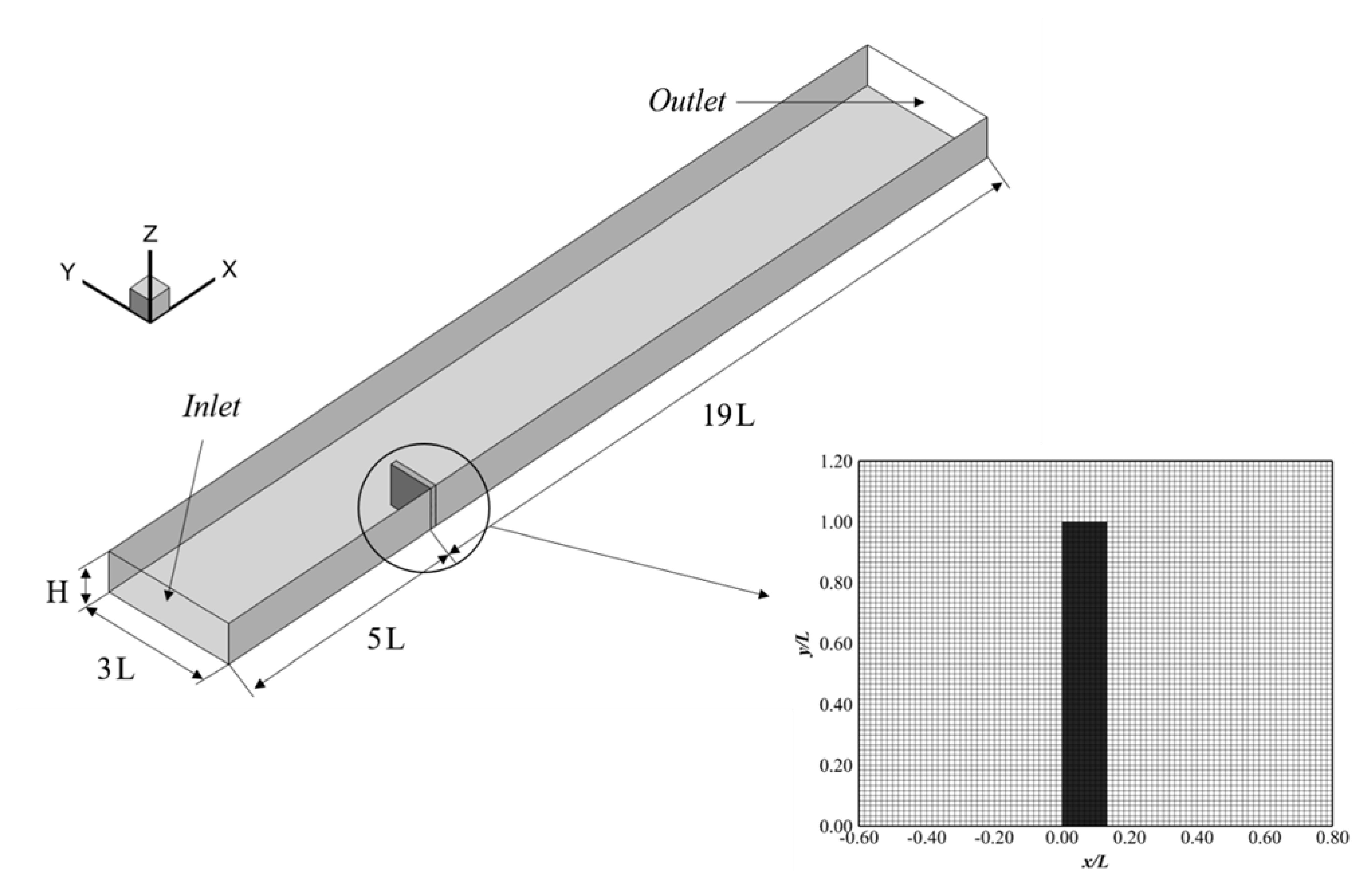
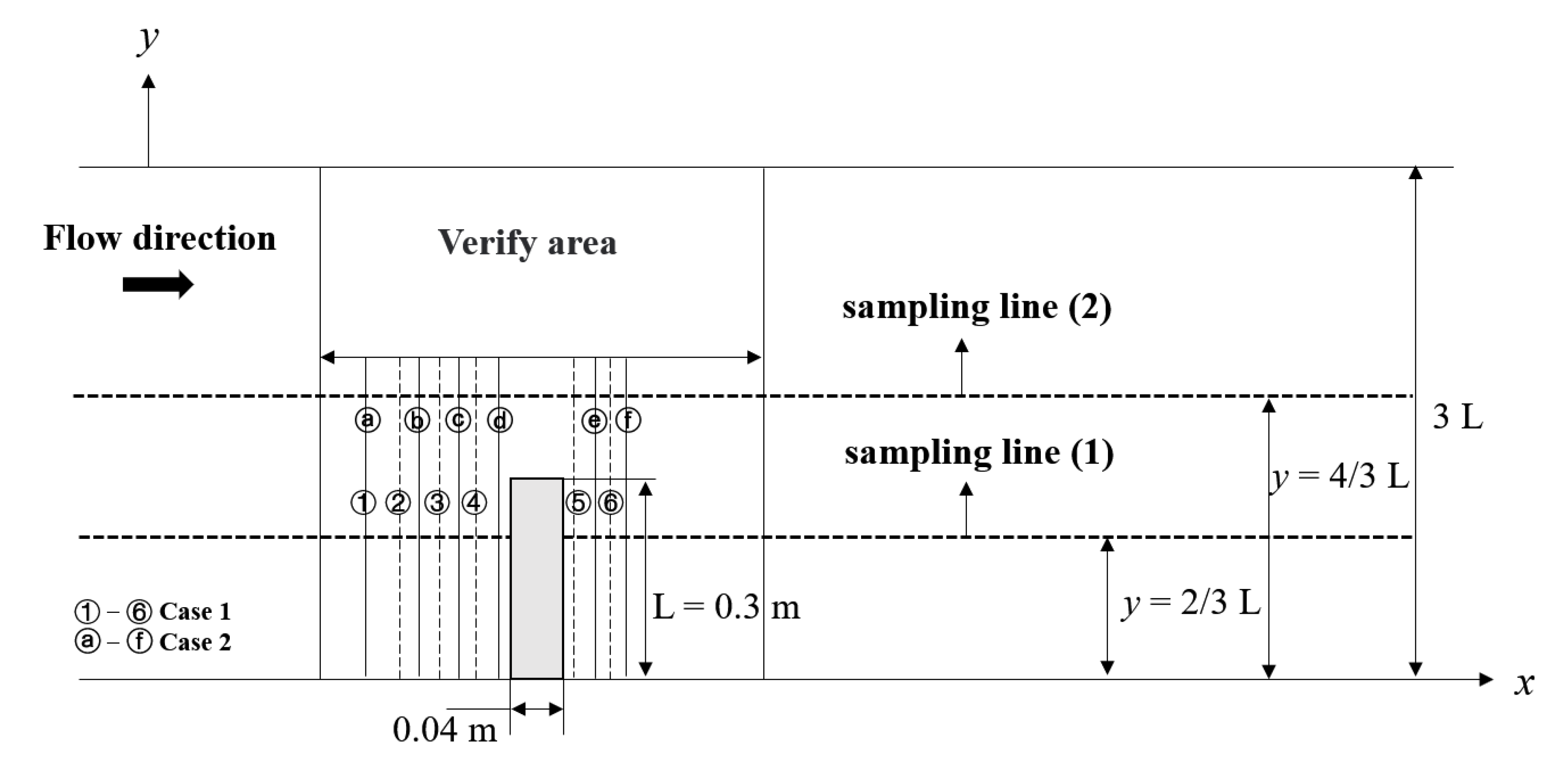
2.2. Computational Setup and Boundary Conditions

Experiments were conducted in a wide, shallow open channel at Hanyang University’s laboratory [33]. The channel was 20 m long and 0.9 m wide, fitted with a model spur dike that stretched across the channel’s height, and the bed slope was 0. The spur dike had length by width dimensions of L = 0.3 m. The parameters in the simulation were set according to the laboratory dimensions, where the installation position of the spur dike was at x = 0 and the uniform flow depth was selected as H = 0.215 m to guarantee the simulation’s reliability. All dimensions were normalized to the length of the spur dike L and the uniform flow depth H. Based on the experimental results, the computational domain spanned 5L upstream of the spur dike and 19L downstream, as depicted in Figure 1, which covered the whole wake region and sufficiently resolved the proposed sequence structure at each scale. The uniform flow bed shear stress was <τ> = 0.142 N/m², which was calculated by taking the average. The Froude number ($Fr=\frac{U_0}{\sqrt{gH}}$) and the Reynolds number ($\mathrm{Re}=\frac{U_{0}H}{\upsilon }$, where 𝜈 is the water kinematic viscosity) were based on the mean velocity U₀ and the water depth H. The flow conditions and simulation variables in both Case 1 and Case 2 are summarized in

Table 1. Hydrological circumstances and computational details.

Case	U0 (m/s)	Q (m3/s)	Re	Fr
1	0.144	0.0278	30,000	0.1
2	0.273	0.0528	65,900	0.19

.

Both Case 1 and Case 2 were created with coarse and fine homogeneous numerical grids. The coarse mesh for Case 1 consisted of about 11.2 billion grid cells. A coarse grid size of dx = dy = dz = 0.01 m was adopted in the streamwise, spanwise, and vertical directions, whereas the fine grid increased the resolution in all directions by a factor of two, leading to about 22.4 billion grid cells when the OpenMP/MPI partitioning approach was used to parallelize the processing. The resolution of the grid for computations involving wall units y+ was 20. The wall function was used to estimate the velocity distribution near the wall. The accuracy of the wall’s turbulent flow prediction was influenced by the precision of the description of the near-wall flow. The grid size was precise enough to construct the first layer of wall grids at the viscous bottom layer. To ensure that the LES simulation of near-wall flow conformed to physical laws, the WALE model did not incorporate an additional eddy viscosity effect near the wall. The computational domains are discretized using grids with consistent spacing. Figure 1 also shows the computational grid (for clarity, only the local fine grid line around the spur dike is plotted).

The velocity boundary was adopted at the inlet of the numerical model, and the inflow of the model was fully developed turbulence based on artificial vortex technology [14]. At the domain’s outflow, the convective boundary condition was utilized to guarantee that coherent structures departed the domain without producing non-physical oscillations. By using wall functions, a no-slip condition was applied to the near-wall velocities of the other solid boundaries. Because of the characteristics of the free liquid level of the flow, the treatment of the free liquid level was particularly difficult and crucial in the numerical simulation. The relatively stable free water surface could be simplified and approximated by the assumptions of the rigid-lid method, which has very important engineering value and academic significance for the accurate analysis of the free liquid level. The rigid-lid method has been used in studies of open channel flow, and many studies have shown that it can accurately simulate free liquid levels [41]. As the Froude numbers of the examined scenarios fell below 0.5, the free surface was treated as a shear-free rigid lid [28]. The change in the free surface was only about 1–2% in both cases, so the rigid-lid assumption could be adopted for the free surface. The simulation was initially run for a period of 2 flows through time (T = l/U₀, l is the channel length) to develop the flow and was then continued for another 50 T to acquire first-order and second-order statistics, which could obtain reasonably accurate time-averaged values.

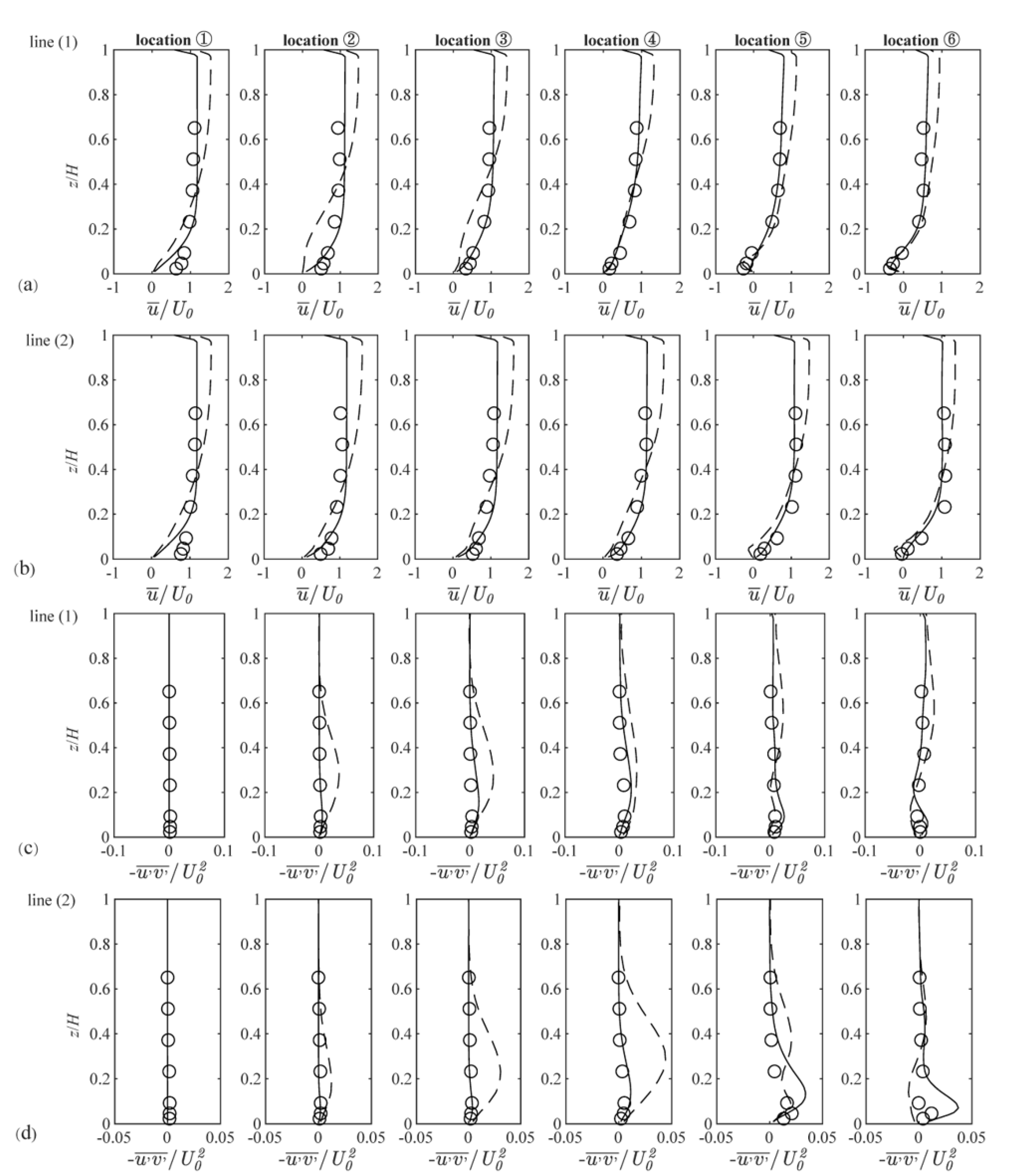
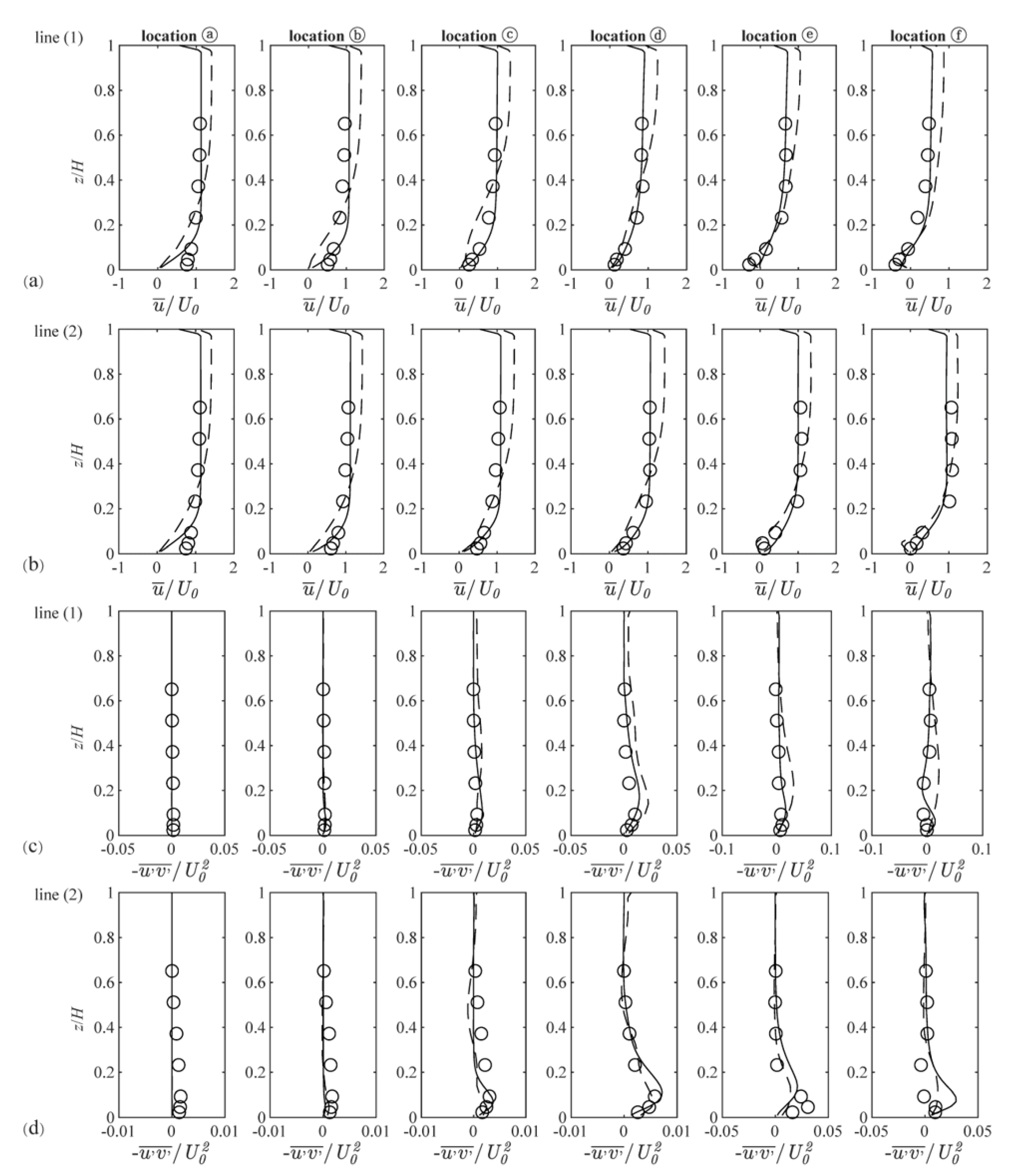
2.3. Model Validation

In this part, the LES predictions for the spur dike in Case 1 and Case 2 were compared with the laboratory data to illustrate the predictive ability of the LES method. The present simulation was verified using Jeongseok’s ADV experiment [33]. The top view of the location of the measured points is shown in Figure 2, in which the intersections between the selected sampling lines (1) and (2) and (Case 1) the dashed line and (Case 2) the solid line represent the location of the measurement points extracted in Figure 3 and Figure 4. Each sampling line along the direction of the flow contained six measurement points in both Case 1 (①–⑥) and Case 2 (a–f). Figure 3 and Figure 4 present the profiles of the calculated time-averaged velocity and turbulence stress at the places shown in Figure 2, for a total of 12 measured points in each case.

The simulations of time-averaged velocity and turbulence stress were verified with experimental data. Furthermore, all measurement points in the experiment were verified, and the verification results were similar in Case 1. For simplicity, only part of the simulation results for the selected sampling lines has been shown for verification. For both Case 1 and Case 2, Figure 3 and Figure 4 show the dimensionless time-averaged streamwise velocity and the primary shear stress of the measurement points along the direction of water depth. Moreover, the vertical coordinate z was normalized by the water depth H, the experimental data were represented by circles, the dashed lines represented coarse-grid LES, and the solid lines represented fine-grid LES. Both grids accurately forecasted the values of streamwise velocity and primary shear stress shown in Figure 3 in both cases. The deviation may be because the change in the free liquid level was ignored in the shear-free rigid lid, and there was a certain fluctuation in the water level near the spur dike. In addition, fine mesh and coarse mesh were compared to examine grid resolution convergence for both cases. Overall, the correlation between the experimental data and the LES findings was excellent. The estimated result closely matched the observed results, and the method could capture the characteristics of turbulence under contraction of the flow by using both grids. The accuracy of the LES results improved with increasing grid refinement, and the fine mesh simulation provided a better agreement with the experimental data. Near the wall, the fine grids had a greater resolution and more accurate forecasts, confirming that the fine grid was sufficiently fine to offer an accurate depiction of the flow field for Case 1 and Case 2. because of the increased resolution. The subsequent graphs in this work are based on the dataset produced from simulations with the fine mesh.

3. Results and Discussion

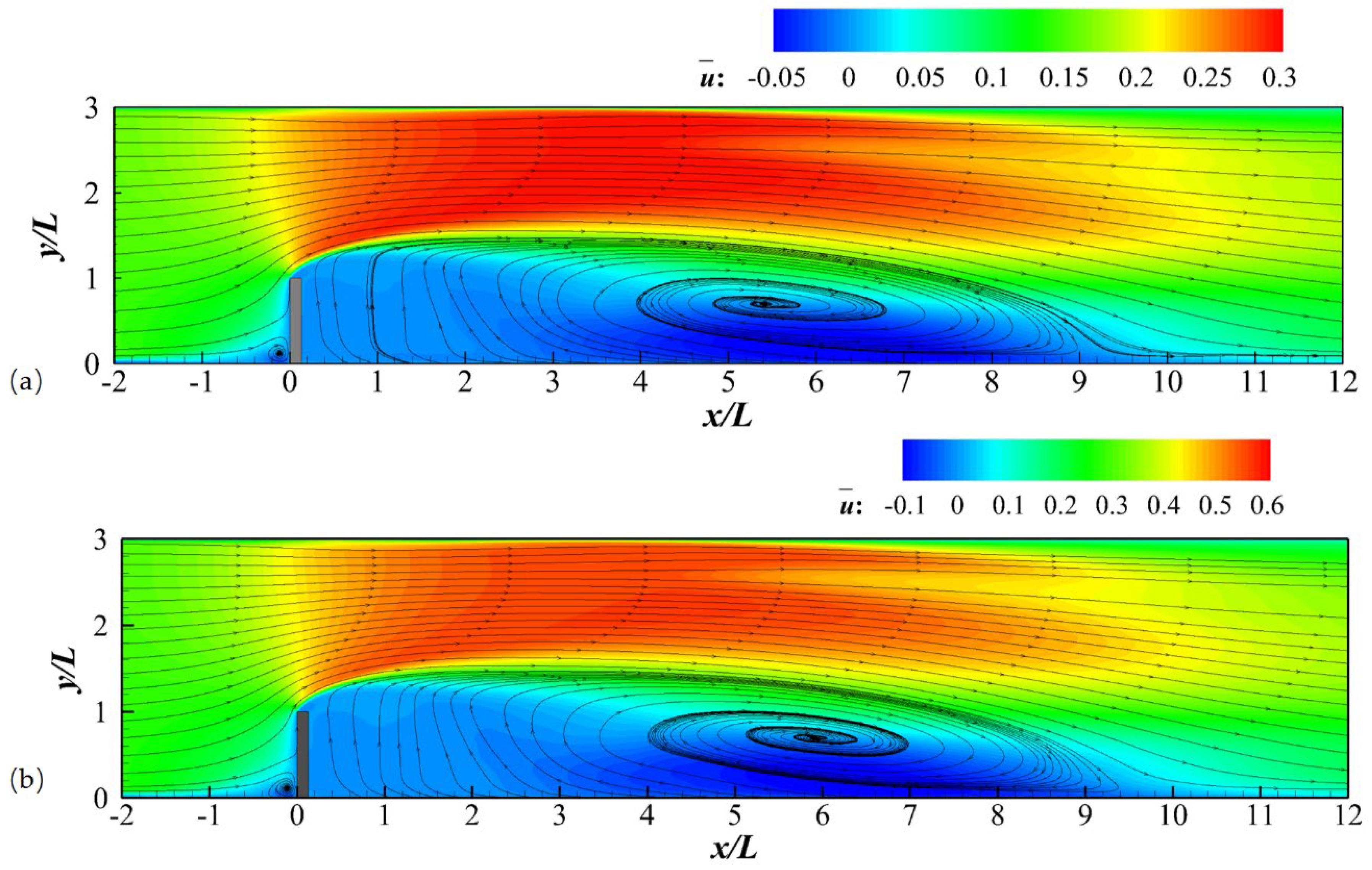
3.1. Time-Averaged Flow

Figure 5 depicts the contours of streamwise velocity at z/H = 0.05. The two-dimensional flow field was extracted at z/H = 0.05 above the depth of flow in the channel. The zone of negative streamwise velocity downstream from the spur dike, as shown in the zero streamwise velocity contour, was formed by the flow separation. Moreover, flow separation processes are the reason a larger recirculation zone is formed. The mainstream area is plotted in red, while the negative flow rates in the recirculation area are shown in blue in Figure 5a,b. The flow gradients in both cases followed the same trend. The time-averaged streamwise velocity along the mainstream area was about 0.3 m/s in Case 1, which was half of that in Case 2. To fully resolve the hydrodynamic characteristics in the vicinity of the spur dike, the streamlines were used to describe the distribution of the vortex. There was an adherent corner vortex upstream of the spur dike in Figure 5a,b, which has been confirmed in experiments [33]. However, the form of the streamline as influenced by the Froude number was not significant within a certain range. The recirculation bubble was controlled by one main vortex. When the incoming flow increased twofold, the area of the downstream recirculation zones increased slightly, where the reattachment streamline was located approximately between x/L = 9 and 10 in Case 1 and Case 2, respectively.

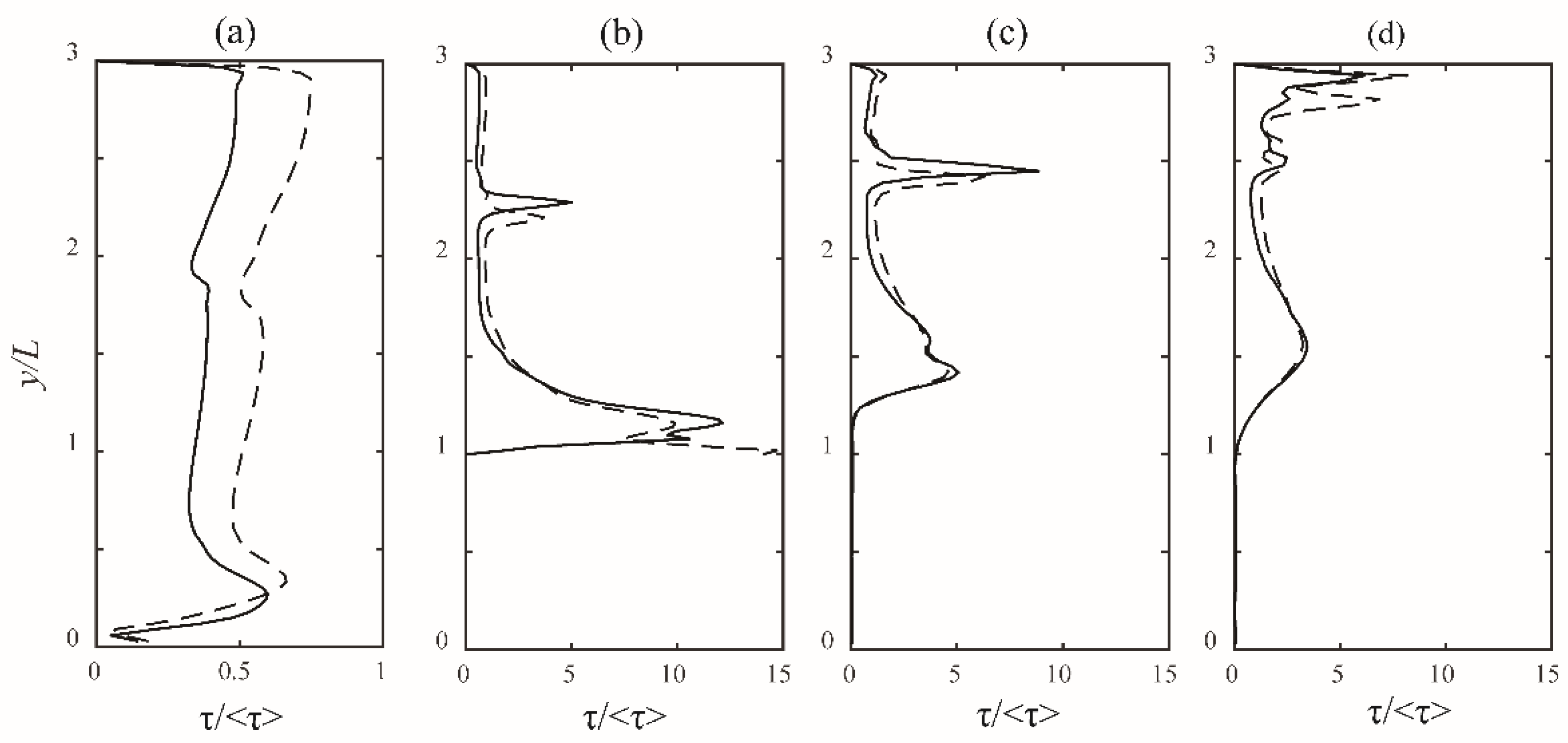
3.2. Bed Shear Stress

Regarding sediment-transport-related processes, the comparisons between Case 1 and Case 2 emphasized the flow towards the bed, i.e., at z/H = 0.05, where the impacts of the free-surface deformation were least pronounced. Figure 6 presents the profiles of the bed shear stress at selected locations near the spur dike, i.e., x = −1, 0, 1 and 2. The bed shear stress was normalized by the uniform flow bed shear stress. In Figure 6, the dashed line represents the results of LES in Case 1 and the solid lines represent the results of LES in Case 2. The bed shear stress increased from y/L = 1, which was the result of the damping effect of the spur dike, where the flow accelerated in the mainstream zone [42]. The leading edge of the spur dike, at x = 0, shows higher bed shear stresses in Figure 6b, where the peak of the bed shear stresses appears near the separated shear layer. This is associated with the creation of a powerful shear layer, which can also lead to a high level of turbulent kinetic energy. Below y/L = 1, negative velocities occurred in the recirculation zone, caused by the backwater effect. The bed shear stress was generally low upstream from the spur dike, as shown in Figure 6a. This corresponds to the findings of Koken et al. [29,43], which showed high riverbed shear stress values near the tip of the dam, upstream from the detached shear layer and below the main chain vortex. The solid and dashed lines show similar trends, indicating that the changes in bed shear stress are similar.

The bed shear stresses presented a bimodal distribution which can be observed in Figure 6. When the position of the sampling line was far away from the spur dike, the peak value gradually approached the mainstream area. As shown in Figure 6c, the main peak value occurred at y/L = 2.4, and the next level peak occurred at y/L = 1.4. As a comparison, in Figure 6d, the main peak value occurred at y/L = 2.9, and the next level peak occurred at y/L = 1.6. In both cases, the location where the peak value occurred was similar. In general, the maximum bed shear stress was caused by horseshoe vortices near the spur dike’s leading edge.

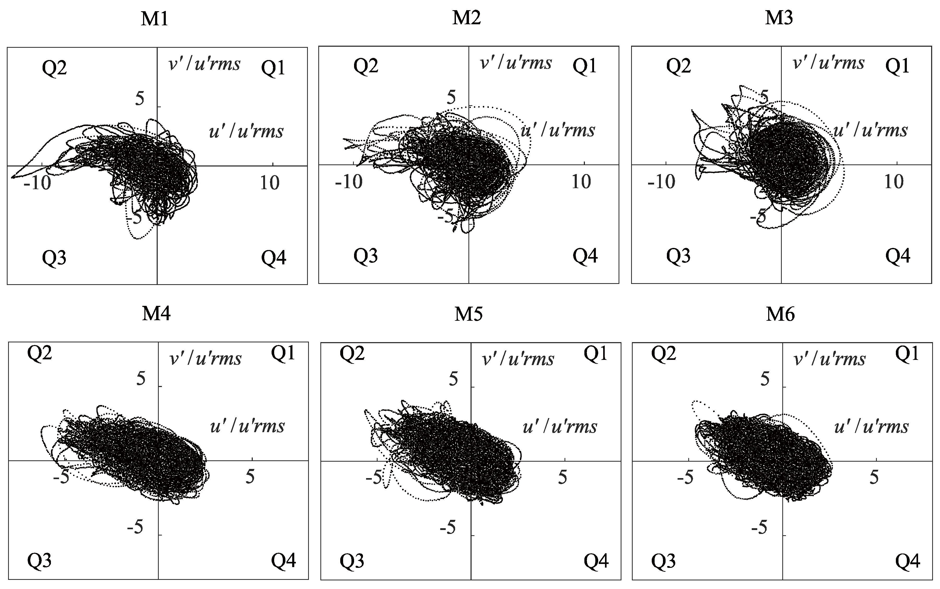
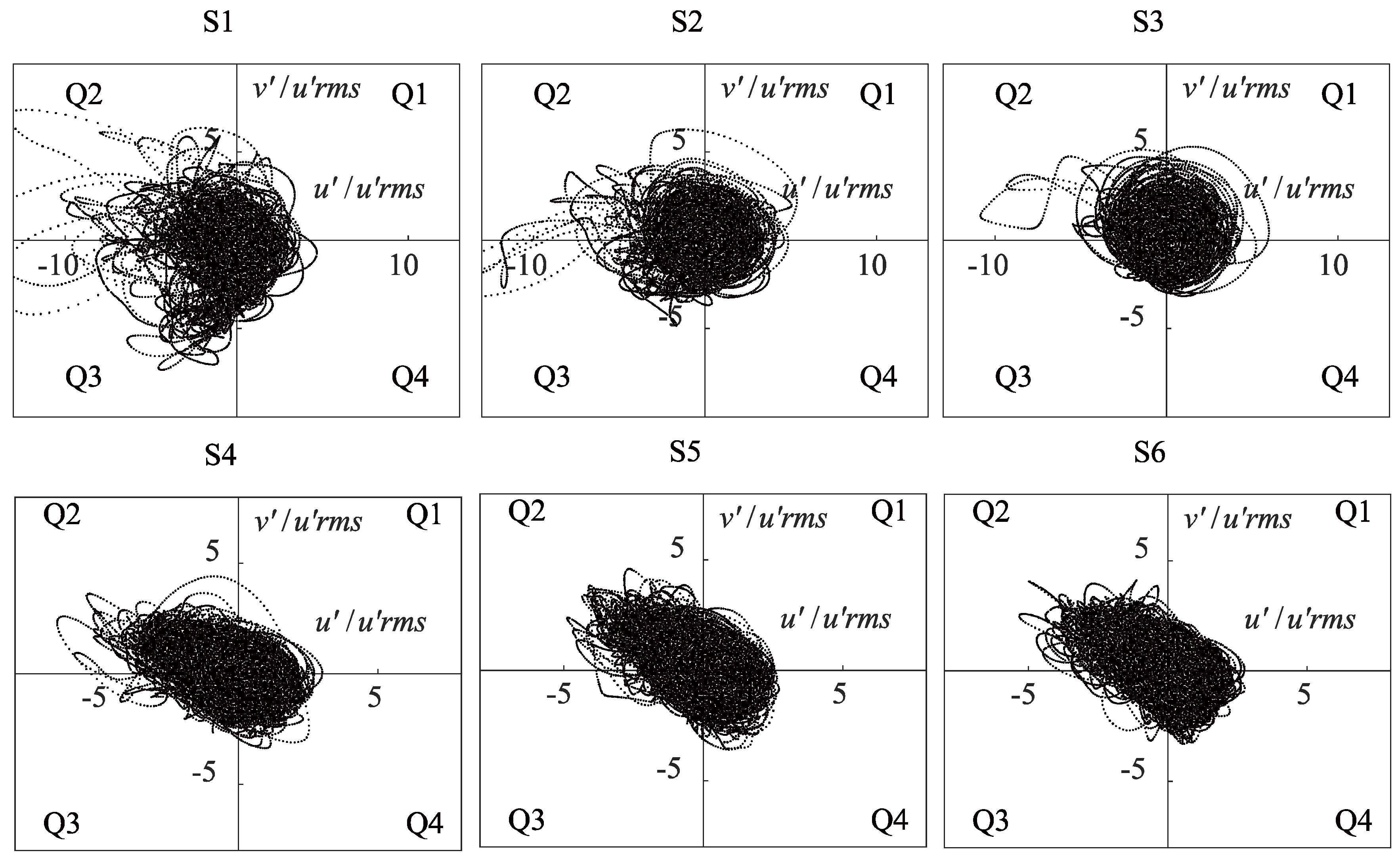
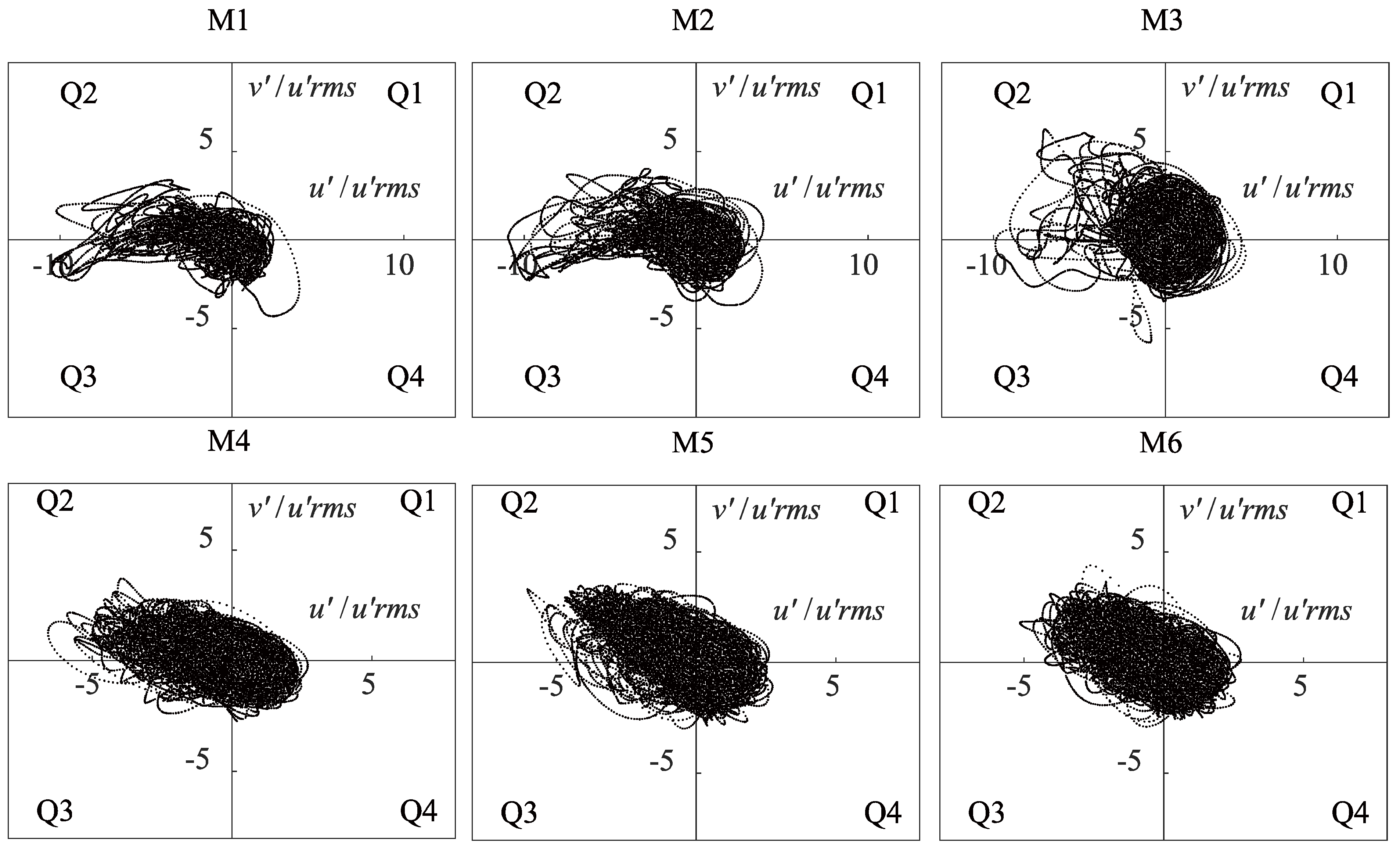
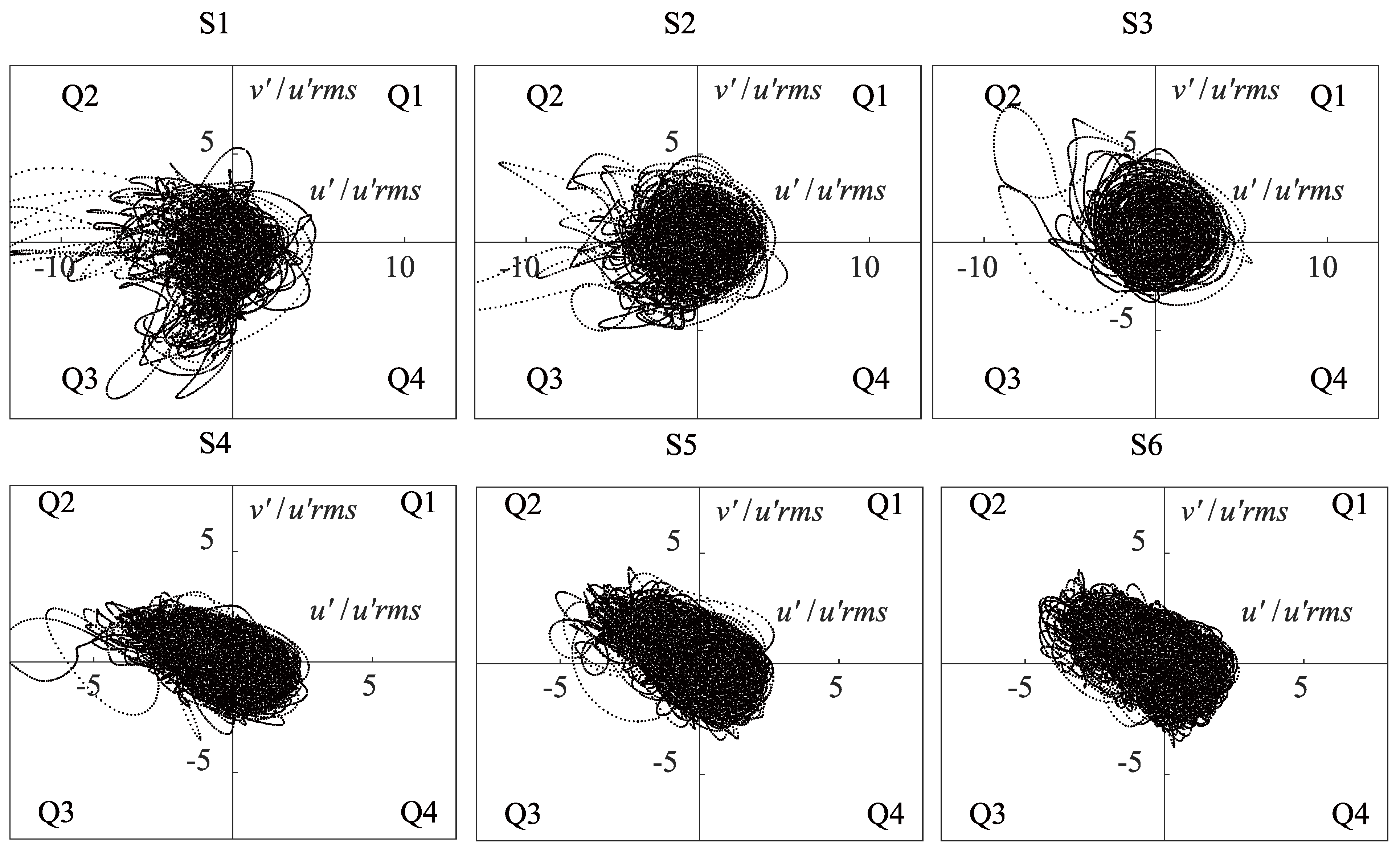
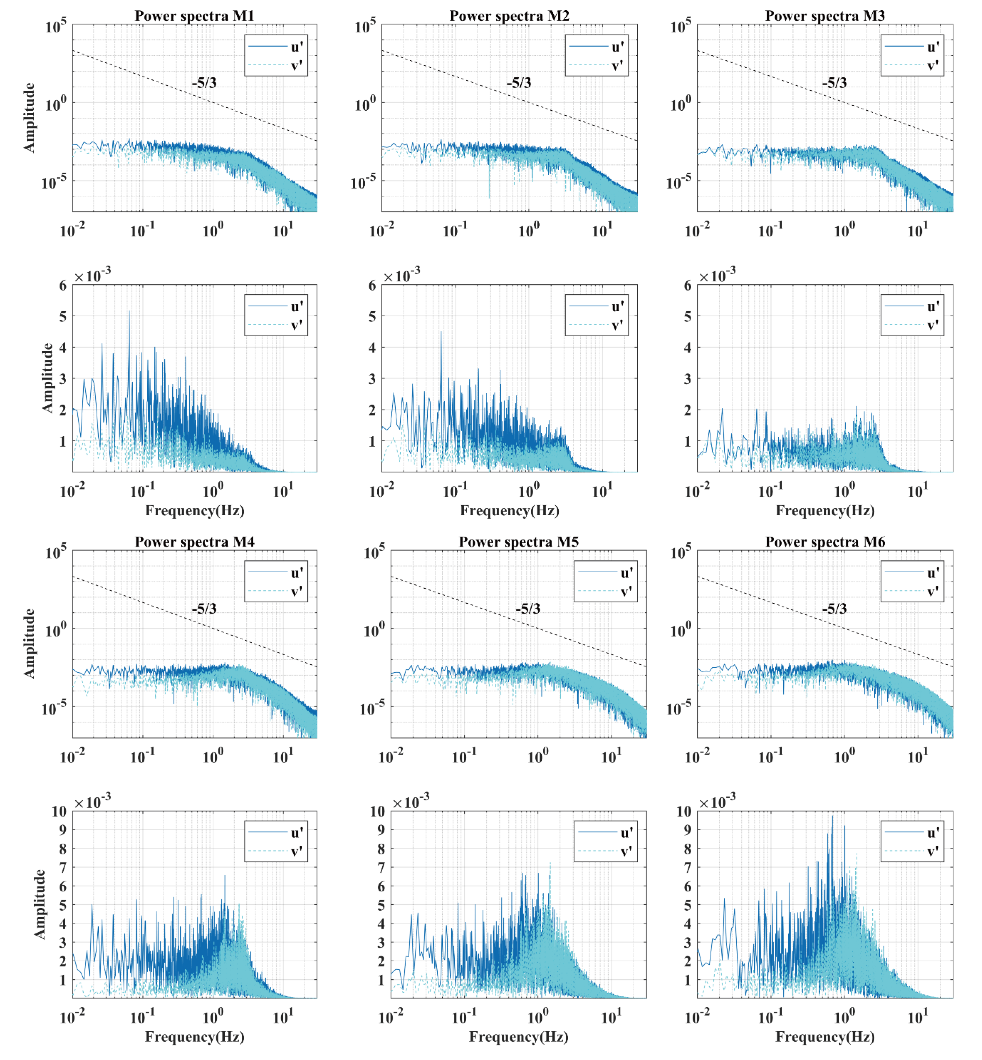
3.3. Second-Order Turbulence Statistics

Turbulent structures in the detached shear layer can induce a large local value of the bed shear stress [43]. In order to further explore the local high bed shear stress shown in Figure 6, this study focused on the area where the peak was generated, related to strong shear layer formation to quantify the oscillations and vortex volumes developed in the detached shear layer at various discharge levels. Specifically, the turbulent flow characteristics in the vicinity of the detached shear layer attachments at different distances along the profile from the bed were investigated by taking the turbulence statistics at the representative measurement points, where the velocity fluctuation time signals were recorded.

The top view of the position of the measurement points is shown in Figure 7, and the same coordinates were selected in Case 1 and Case 2. These points were taken from midwater and surface layers to better capture the flow characteristics at the junction of the recirculation and mainstream zones. In Figure 7, the coordinates of 1-6 represent the plane location of six points per water layer. There are a total of 12 points per case, including a set of midlevel sampling points and a set of surface sampling points. The velocity components of several time series were captured at 12 sample points and used to simulate a lengthy period. The turbulence properties of these 12 sites in both cases were then examined statistically using probability density functions, quadrant analysis, and spectrum analysis.

Figure 8 plots the probability density function (PDF) of the streamwise velocity fluctuations near the leading edge of the spur dike at all locations. Figure 8 contains four sub-plots representing the PDF distribution of midwater and surface water under Case 1 and Case 2. At each sample point, the probability density function of turbulence fluctuation u′ was computed and normalized by the root mean square value u′_rms. Furthermore, the difference in the probability density functions of the streamwise velocity fluctuations between the midwater and surface layers is shown separately for both cases. The solid line in the four sub-plots of Figure 8 indicates a Gaussian normal distribution. Compared with a normal distribution, the majority of PDFs are skewed towards the positive in both cases, where the high-momentum jets occur, exhibiting oscillation between the recirculation and the main flow. Greater deviation from the normal distribution at the midwater points is shown in Figure 8a,c, indicating slightly different turbulence patterns in the midwater and surface layers. In general, almost all points exhibited a normal distribution, except for M1 and S1, where the peak occurred at approximately u′/u′_rms = −0.2~0.2. M1 and S1 are located close to the top of the spur dike, where small eddies begin to roll up. All other points shown in Figure 8 had a significant skewness and were normally distributed until u′/u′_rms = −1.5, reaching a maximum around u′/u′_rms = 0.5, followed by a sharp decline. This was because the vortex’s energy flow is random and the PDF conforms to a Gaussian distribution. Because of the narrow section bundle with stronger acceleration, the flow started to separate from the spur dike’s tip, where the originally low frequencies often occur with the emergence of the recirculation zone. Obviously, the effect of changes in the flow rate on the form of the turbulence fluctuations is not significant in Figure 8b,d.

Quadrant analysis is widely used to analyze turbulent structures [44]. The next part of the study examined the changes in the turbulence characteristics across various flow conditions, with an emphasis on the differences at different flow depths. Quadrant analysis was used by Lu and Willmarth [45] to identify the presence of coherent structures in the flow and to quantify their contribution to Reynolds shear stress. This study, unlike standard quadrant analysis near the bed in previous research, was conducted to analyze the horizontal turbulence events in the vicinity of the detached shear layer. In particular, this segregation may identify structures that contribute positively to Reynolds stress and those that provide a negative contribution (outward (Q1) and inward (Q3) interactions) [46].

The plane is shown in Figure 9, with four quadrants consisting of streamwise and spanwise velocity fluctuations, reflecting the frequency of various turbulence events and their contribution to the formation of Reynolds shear stresses [47]. Each quadrant in Figure 9, Figure 10, Figure 11 and Figure 12 represents the occurrence of different turbulence events. Strong turbulence in large shallow open channels with a spur dike is mostly a result of streamwise and spanwise velocity fluctuation, so vertical velocity fluctuations have been omitted, and only the results of streamwise and spanwise velocity fluctuations are displayed. The differences in the horizontal turbulence structure between the midwater and surface waters were analyzed here. The horizontal coordinate represents the streamwise velocity fluctuations standardized by the root mean square value, while the vertical coordinates represent the spanwise velocity fluctuation standardized by the root mean square value. We considered the flow direction as the positive direction. The first quadrant represents the outward motion of the high-velocity fluid (Q1: u′ > 0, v′ > 0). The second quadrant represents when the vortex started to emerge (Q2: u′ < 0, v′ > 0). The third quadrant represents the inward motion of a low-velocity fluid (Q3: u′ < 0, v′ < 0). The fourth quadrant represents the continuing development of the vortex (Q4: u′ > 0, v′ < 0). The pulsating flow structure is directly connected to the momentum exchange of the flow. Two types of turbulent flow, Q2 and Q4, shown in Figure 9, Figure 10, Figure 11 and Figure 12, controlled the generation and maintenance of turbulence near the recirculation zone.

Figure 9 plots the quadrant analysis of the streamwise and spanwise velocity fluctuation normalized for Case 1 at z/H = 0.51, including the six sampled locations M1–M6 shown in Figure 7. At M1, most points are located in the second and fourth quadrants, which indicates that the Q2 and Q4 events are the dominant occurrences related to the formation and development of the vortex. This phenomenon means that it made the largest contribution to the generation of $-\overline{u^{\prime }{v}^{\prime }}$. Furthermore, it exhibited more balanced isotropy at M2 and M3, where the sustainable development of a vortex occurs in a separate shear layer. M2 is more diffuse than M3, having a wider range of variance in turbulence. At M2 and M3, numerous points are located in the first (u′ > 0, v′ > 0) and third quadrants (u′ < 0, v′ < 0), related to the ejection of flow and the intrusion of low-frequency circulating flow in the shear layer. The spur dike reduces the width of the riverbed, thus increasing the velocity of the water flow so that a recirculation bubble occurs downstream from the spur dike, which can be observed in Figure 5. Points M4, M5, and M6 produced a more symmetrical elliptical structure, dominated by the appearance of Q2 and Q4, where the maximum energy transfer takes place. As shown in Figure 9, the variation in the streamwise velocity fluctuations between positive and negative illustrates the changes in the bending of detached shear layers close to the spur dike, and the same conclusion can be found in Figure 10, Figure 11 and Figure 12. Turbulent anisotropy initiates secondary flows, redistributes the mass and momentum within a cross-section, or strengthens and preserves the coherence of particularly turbulent structures; hence, the anisotropy of turbulent flows is of enormous interest to scientists and engineers.

Figure 11 shows the results of the quadrant analysis at increasing flow rates. At M1 and M2 in Figure 11, most points are located in Quadrants 2 and 4 and closer to the axis, indicating greater one-dimensionality. At M3 in Figure 11, compared with the point at z/H = 0.51 in Figure 9, the second quadrant of the velocity fluctuation shows a higher range of change than the other quadrants, which looks more stable. This is a result of the current’s more extreme stretching of the water column and its more violent momentum transition. Figure 9 and Figure 11 show comparable outcomes between Case1 at z/H = 0.51 and Case 2 at z/H = 0.51 and show that the form of the turbulent structure at the separated shear layer was not significantly affected by the flow rate. As the flow velocity increases, the current is constricted more strongly. These phenomena and the conclusions for Case 1 and Case 2 at z/H = 0.93 are similar and are shown in Figure 10 and Figure 12.

The periodicity of the vortices was investigated by spectral analysis. Figure 13 and Figure 14 plot the power spectra of the streamwise and spanwise velocity fluctuation time series at all locations in Case 1 and Case 2. The figure below each logarithmically processed plot corresponds to a semi-logarithmically processed spectral analysis plot. Semi-logarithmic coordinates provide a good view of the magnitude and periodicity of the energy. The results of spectral analysis for all points approximated the −5/3 slope in the logarithmic coordinates of Figure 13 and Figure 14, showing homogeneous turbulence before a quicker decay of energy was found at higher frequencies, which was largely produced by the sub-grid scale (SGS) model [48]. Due to the control of the Kolmogorov scale, the velocity spectral density function in the open channel flow contained a 0 slope with the largest vortex in the energy-containing interval, and a slope of −5/3 with successively smaller vortices in the inertial sub-interval, and a steeper slope with the smallest vortices in the dissipative interval [49]. This was determined by spectral analysis of a time series of velocity variations, and it is evident from Figure 13 and Figure 14 that these three slopes range between 0 and −5/3, with a wider frequency range in the −5/3 slope range.

Figure 10 and Figure 12 sequentially plot the quadrant analysis of the streamwise and spanwise velocity fluctuations normalized by u′_rms for both cases at z/H = 0.93, including the sampled locations S1–S6 in both cases. Figure 10 and Figure 12 further reveal the turbulent structure in the surface waters. Thus, the difference in the turbulence statistics at various water depths is also illustrated by comparing the analysis results of Figure 9 and Figure 10, Figure 11 and Figure 12. In surface waters, current stretching is more severe, and momentum transfer is more evident. S1 in Figure 12, unlike M1 in Figure 11, exhibits more homogeneity and a greater range of variation in the velocity fluctuation. Points S4, S5, and S6 in Figure 12 also produce a more symmetrical oval structure controlled by the events of Q2 and Q4. Moreover, the same distinction among the six points can be observed in Figure 9 and Figure 10.

Figure 13 shows the results of the analysis of power spectra in Case 1. At positions M1–M3, the vortex starts to form with overall low energy, but at positions M4–M6, the energy increases significantly, and the vortex continues to develop, corresponding to the results of the quadrant analysis. As shown in Figure 13, a considerable part of the kinetic energy is concentrated at frequencies between 0.1 and 1 Hz. In other words, the dominant frequency of turbulence in Case 1 is between 0.1 and 1 Hz. The majority of the energy peak occurs at f = 0.3–0.5 Hz. Furthermore, a significant portion of the kinetic energy is focused on frequencies between 0.1 and 8 Hz, as shown in Figure 14, which illustrates higher energy with the increase in the flow rate. The amplitude of the power spectrum in Case 2 is twice that of Case 1, proportional to the increase in the flow. Moreover, the occurrence of maximum energy is located at the peak frequency of 0.8–1 Hz in Case 2, as shown in Figure 14.

Figure 13 and Figure 14 indicate that the inertial sub-range of the energy cascade for u′ and v′ was well resolved, and that the energy-containing scales of the flow were resolved adequately by the fine grids [48]. All spectra have a zone with slopes of −5/3 for frequencies in the inertial region and above, which can be observed by log–log scale in Figure 13 and Figure 14. These findings suggest the presence of two-dimensional vortical structures with an inverted cascade of turbulent energy [50]. This verified the transmission of energy from minor eddies to huge vortical formations. In turbulence, energy is mostly lost at small scales (large wave numbers), and hence, energy is transported from large scales (small wave numbers) to small scales (large wave numbers) to compensate for this loss. Thus, energy is simply transferred from one scale to another at relatively large sizes [51,52]. These turbulent dynamics correlate to those shown in Figure 15 in the recirculation area of the detached shear layer where the emergence, development, migration, and merging of whirlpools take place. Turbulent energy is mainly controlled by horizontal turbulence.

The results were also calculated for the spectral analysis at points of the surface water (z/H = 0.93) location in Case 1 and Case 2. For simplicity, only the power spectrum of the point at the location of z/H = 0.51 is shown here, as the results observed at z/H = 0.93 were similar. Despite the differences in the structural form of turbulence in the quadrant analysis for differences in water depth, the power spectra of flow velocity fluctuations did not differ significantly, exhibiting the same periodicity for the vortex and energy transmission.

3.4. Instantaneous Turbulent Flow Structures

Q-criteria for observing the formation and separation of isolated shear layer eddies downstream of spur dikes for both Case 1 and Case 2 are shown in Figure 15a,b. These provide a top view of a transient turbulent structure denoted by the iso-surfaces of the q-criterion, a scalar that emphasizes the region of the flow when the strain is dominated by rotation, which is colored by the normalized time-averaged streamwise flow velocity to highlight the kinetic energy carried by the vortex; here, Q = 100 for both cases. The Q-criterion can allow the shapes and vorticity to be observed, which are shown in Figure 15. The horseshoe vortex near the tip of the spur dike is responsible for the maximum bed shear stress profile, which can also be noticed in Figure 6b. Figure 15 shows the coherent structures downstream of the spur dike, where eddies can be observed. Most of the vortex trajectory is essentially parallel to the incoming flow. The horseshoe vortex system forms when the flow divides at the tip of the spur dike, and vortices progressively form and grow close to the separated shear layer, which is similar to the results of a wall-mounted cube observed by Yakhot et al. [51]. Near the tip of the spur dike, the horseshoe eddies are very similar in size in both cases, along with the stretching of the vortex. In Case 2, the dominant coherent structure is more consistent and increases the number of vortices depicted in Figure 15b.

Some vortices with low kinetic energy also occur in the recirculation zone near the areas downstream from the spur dike. The high-momentum vortices are mainly located at the junction of the mainstream and recirculation zones, where the momentum exchange takes place. In Case 1, the vortex in the wake area bends towards the recirculation zone below the spur dike, as shown in Figure 15a. The vortex is randomly brought into the recirculation area behind the spur dike. Due to flow separation, shedding vortices appear in the wake of the downstream spur dike. This phenomenon can be observed in Figure 15b.

4. Conclusions

The study has investigated the effect of incoming flow velocity on the flow around a spike dike by comparing and discussing the results of two large-eddy simulations. Setup and boundary conditions were chosen in analogy to a laboratory experiment to ensure validation of the LES’ capability to accurately reproduce such flows. Good agreements between LESs and experimental measurement were found along different gauging lines, and additional turbulence statistics were extracted from the simulations, demonstrated, and discussed. Large local values of bed shear stress can be induced by turbulent structures in the detached shear layer. Greater deviation from the normal distribution in both Case 1 and Case 2 was shown by the probability density functions, which exhibited clear positive skewness. The result illustrated a more symmetrical elliptical form controlled by occurrences of Q2 and Q4, where the maximum energy transfer took place. The energy of turbulence is concentrated on the location of vortex development. However, the results of the power spectra displayed the same periodicity for the vortex and energy transmission, despite variances in the structural form of turbulence in the quadrant analysis at different water depths. An increase in the flow rate merely enhanced the energy transfer.

The study focused on the differences in the horizontal two-dimensional turbulence and the vortex structure of the separated shear layer at different distances from the bed, which is different from traditional research. Our methods and findings also significantly advance our knowledge of the vortex structure of the separating shear layer and contribute to previous studies on the turbulence characteristics near spur dikes, which fill in the gaps in experimental studies.

References

1. Bernhardt, E.S.; Palmer, M.A.; Allan, J.D.; Alexander, G.; Barnas, K.; Brooks, S.; Carr, J.; Clayton, S.; Dahm, C.; Follstad-Shah, J.; et al. Synthesizing U.S. River Restoration Efforts. Science 2005, 308, 636–637. [Google Scholar] [CrossRef]
2. Bice, C.M.; Gibbs, M.S.; Kilsby, N.N.; Mallen-Cooper, M.; Zampatti, B.P. Putting the “River” Back into the Lower River Murray: Quantifying the Hydraulic Impact of River Regulation to Guide Ecological Restoration. Trans. R. Soc. South Aust. 2017, 141, 108–131. [Google Scholar] [CrossRef]
3. Bunn, S.E.; Arthington, A.H. Basic Principles and Ecological Consequences of Altered Flow Regimes for Aquatic Biodiversity. Environ. Manag. 2002, 30, 492–507. [Google Scholar] [CrossRef] [PubMed] [Green Version]
4. Lamouroux, N.; Gore, J.A.; Lepori, F.; Statzner, B. The Ecological Restoration of Large Rivers Needs Science-based, Predictive Tools Meeting Public Expectations: An Overview of the Rhône Project. Freshw. Biol. 2015, 60, 1069–1084. [Google Scholar] [CrossRef]
5. Chanson, H. Utilising the Boundary Layer to Help Restore the Connectivity of Fish Habitats and Populations. An Engineering Discussion. Ecol. Eng. 2019, 141, 105613. [Google Scholar] [CrossRef]
6. Sun, Z.; Sun, W.; Tong, C.; Zeng, C.; Yu, X.; Mou, X. China’s Coastal Wetlands: Conservation History, Implementation Efforts, Existing Issues and Strategies for Future Improvement. Environ. Int. 2015, 79, 25–41. [Google Scholar] [CrossRef]
7. Kang, J.; Yeo, H.; Jung, S. Flow Characteristic Variations on Groyne Types for Aquatic Habitats. Engineering 2012, 4, 809–815. [Google Scholar] [CrossRef] [Green Version]
8. Kilsby, N. Reach-Scale Spatial Hydraulic Diversity in Lowland Rivers: Characterisation, Measurement and Significance for Fish. Ph.D. Thesis, University of Adelaide, Adelaide, SA, Australia, 2008. [Google Scholar]
9. Walker, K. Serial Weirs, Cumulative Effects: The Lower River Murray, Australia; Cambridge University Press: Cambridge, UK, 2006; pp. 248–279. [Google Scholar]
10. Baxter, R.M. Environmental Effects of Dams and Impoundments. Annu. Rev. Ecol. Syst. 1977, 8, 255–283. [Google Scholar] [CrossRef]
11. Im, D.; Kang, H. Two-Dimensional Physical Habitat Modeling of Effects of Habitat Structures on Urban Stream Restoration. Water Sci. Eng. 2011, 4, 386–395. [Google Scholar] [CrossRef]
12. Dong, Z.-R.; Sun, D.-Y.; Zhao, J.-Y.; Zhang, J. Progress and Prospect of Eco-Hydraulic Engineering. J. Hydraul. Eng. 2014, 45, 1419–1426. [Google Scholar] [CrossRef]
13. Mehraein, M.; Ghodsian, M. Experimental Study on Relation between Scour and Complex 3D Flow Field. Sci. Iran. 2017, 24, 2696–2711. [Google Scholar] [CrossRef] [Green Version]
14. Deng, Y.; Cao, M.; Ma, A.; Hu, Y.; Chang, L. Mechanism Study on the Impacts of Hydraulic Alteration on Fish Habitat Induced by Spur Dikes in a Tidal Reach. Ecol. Eng. 2019, 134, 78–92. [Google Scholar] [CrossRef]
15. Kuhnle, R.A.; Jia, Y.; Alonso, C.V. Measured and Simulated Flow near a Submerged Spur Dike. J. Hydraul. Eng. 2008, 134, 916–924. [Google Scholar] [CrossRef]
16. Alauddin, M.; Hossain, M.M.; Uddin, M.N.; Haque, M.E. A Review on Hydraulic and Morphological Characteristics in River Channels Due to Spurs. World Acad. Sci. Eng. Technol. Int. J. Environ. Chem. Ecol. Geol. Geophys. Eng. 2017, 11, 397–404. [Google Scholar]
17. Stoesser, T. Large-Eddy Simulation in Hydraulics: Quo Vadis? J. Hydraul. Res. 2014, 52, 441–452. [Google Scholar] [CrossRef]
18. McCoy, A.; Constantinescu, G.; Weber, L.J. Numerical Investigation of Flow Hydrodynamics in a Channel with a Series of Groynes. J. Hydraul. Eng. 2008, 134, 157–172. [Google Scholar] [CrossRef]
19. Jirka, G.H. Large Scale Flow Structures and Mixing Processes in Shallow Flows. Null 2001, 39, 567–573. [Google Scholar] [CrossRef]
20. Ouro, P.; Stoesser, T. An Immersed Boundary-Based Large-Eddy Simulation Approach to Predict the Performance of Vertical Axis Tidal Turbines. Comput. Fluids 2017, 152, 74–87. [Google Scholar] [CrossRef] [Green Version]
21. Stoesser, T. Physically Realistic Roughness Closure Scheme to Simulate Turbulent Channel Flow over Rough Beds within the Framework of LES. J. Hydraul. Eng. 2010, 136, 812–819. [Google Scholar] [CrossRef] [Green Version]
22. Teruzzi, A.; Armenio, V.; Ballio, F.; Salon, S. Numerical Investigation of the Turbulent Flow around a Bridge Abutment. In River Flow 2006; Alves, E., Cardoso, A., Leal, J., Ferreira, R., Eds.; Taylor & Francis: London, UK, 2006; ISBN 978-0-415-40815-8. [Google Scholar]
23. Shirolé, A.M.; Holt, R.C. Planning for a Comprehensive Bridge Safety Assurance Program. In Proceedings of the 3rd Bridge Engineering Conference, Denver, Colorado, USA, 31 July 1991. [Google Scholar]
24. Chrisohoides, A.; Sotiropoulos, F.; Sturm, T.W. Coherent Structures in Flat-Bed Abutment Flow: Computational Fluid Dynamics Simulations and Experiments. J. Hydraul. Eng. 2003, 129, 177–186. [Google Scholar] [CrossRef]
25. Meselhe, E.; Sotiropoulos, F.; Cao, Z.; Day, R.; Liriano, S. Three-Dimensional Numerical Model for Open-Channels with Free-Surface Variations. J. Hydraul. Res. 2003, 41, 110–111. [Google Scholar]
26. Rajaratnam, N.; Nwachukwu, B.A. Erosion Near Groyne-Like Structures. Null 1983, 21, 277–287. [Google Scholar] [CrossRef]
27. Bomminayuni, S.; Stoesser, T. Turbulence Statistics in an Open-Channel Flow over a Rough Bed. J. Hydraul. Eng. 2011, 137, 1347–1358. [Google Scholar] [CrossRef]
28. Koken, M.; Constantinescu, G. An Investigation of the Dynamics of Coherent Structures in a Turbulent Channel Flow with a Vertical Sidewall Obstruction. Phys. Fluids 2009, 21, 085104. [Google Scholar] [CrossRef]
29. Koken, M.; Gogus, M. Effect of Spur Dike Length on the Horseshoe Vortex System and the Bed Shear Stress Distribution. J. Hydraul. Res. 2015, 53, 196–206. [Google Scholar] [CrossRef]
30. Stoesser, T.; Nikora, V.I. Flow Structure over Square Bars at Intermediate Submergence: Large Eddy Simulation Study of Bar Spacing Effect. Acta Geophys. 2008, 56, 876–893. [Google Scholar] [CrossRef] [Green Version]
31. Jalalabadi, R.; Stoesser, T. Reynolds and Dispersive Shear Stress in Free-Surface Turbulent Channel Flow Over Square Bars. Phys. Rev. E 2022, 105, 035102. [Google Scholar] [CrossRef]
32. Zhao, C.; Ouro, P.; Stoesser, T.; Dey, S.; Fang, H. Response of Flow and Saltating Particle Characteristics to Bed Roughness and Particle Spatial Density. Water Resour. Res. 2022, 58, e2021WR030847. [Google Scholar] [CrossRef]
33. Jeon, J.; Lee, J.Y.; Kang, S. Experimental Investigation of Three-Dimensional Flow Structure and Turbulent Flow Mechanisms Around a Nonsubmerged Spur Dike with a Low Length-to-Depth Ratio. Water Resour. Res. 2018, 54, 3530–3556. [Google Scholar] [CrossRef]
34. Stoesser, T.; McSherry, R.; Fraga, B. Secondary Currents and Turbulence over a Non-Uniformly Roughened Open-Channel Bed. Water 2015, 7, 4896–4913. [Google Scholar] [CrossRef] [Green Version]
35. Stoesser, T.; Kim, S.J.; Diplas, P. Turbulent Flow through Idealized Emergent Vegetation. J. Hydraul. Eng. 2010, 136, 1003–1017. [Google Scholar] [CrossRef]
36. Uhlmann, M. An Immersed Boundary Method with Direct Forcing for the Simulation of Particulate Flows. J. Comput. Phys. 2005, 209, 448–476. [Google Scholar] [CrossRef]
37. Gong, Y.; Mao, J.; Dai, J.; Jiang, D. Large-Eddy Simulation of Turbulent Flow in A Vertical Slot Fishway. In Proceedings of the 7th International Conference on Hydraulic and Civil Engineering & Smart Water Conservancy and Intelligent Disaster Reduction Forum (ICHCE & SWIDR), Nanjing, China, 6–8 November 2021; IEEE: Nanjing, China, 2021; pp. 1302–1306. [Google Scholar]
38. Gong, Y.; Stoesser, T.; Mao, J.; McSherry, R. LES of Flow Through and Around a Finite Patch of Thin Plates. Water Resour. Res. 2019, 55, 7587–7605. [Google Scholar] [CrossRef] [Green Version]
39. Cristallo, A.; Verzicco, R. Combined Immersed Boundary/Large-Eddy-Simulations of Incompressible Three Dimensional Complex Flows. Flow Turbul. Combust. 2006, 77, 3–26. [Google Scholar] [CrossRef]
40. Smagorinsky, J. General Circulation Experiments with the Primitive Equations: I. The Basic Experiment. Mon. Wea. Rev. 1963, 91, 99–164. [Google Scholar] [CrossRef]
41. Kara, S.; Kara, M.C.; Stoesser, T.; Sturm, T.W. Free-Surface versus Rigid-Lid LES Computations for Bridge-Abutment Flow. J. Hydraul. Eng. 2015, 141, 04015019. [Google Scholar] [CrossRef]
42. Hussein, H.J.; Martinuzzi, R.J. Energy Balance for Turbulent Flow around a Surface Mounted Cube Placed in a Channel. Phys. Fluids 1996, 8, 764–780. [Google Scholar] [CrossRef]
43. Koken, M.; Constantinescu, G. An Investigation of the Flow and Scour Mechanisms around Isolated Spur Dikes in a Shallow Open Channel: 2. Conditions Corresponding to the Final Stages of the Erosion and Deposition Process: Flow and Scour Mechanisms, 2. Water Resour. Res. 2008, 44, W08407. [Google Scholar] [CrossRef]
44. Cirlioru, T.M.; Ciocan, G.D.; Barre, S.; Djeridi, H.; Panaitescu, V. Quadrant Analysis of Turbulent Mixing Layer. Rev. Chim. 2013, 64, 326. [Google Scholar]
45. Lu, S.S.; Willmarth, W.W. Measurements of the Structure of the Reynolds Stress in a Turbulent Boundary Layer. J. Fluid Mech. 1973, 60, 481–511. [Google Scholar] [CrossRef]
46. Wiggs, G.F.S.; Weaver, C.M. Turbulent Flow Structures and Aeolian Sediment Transport over a Barchan Sand Dune: Turbulent Structures Over Aeolian Dunes. Geophys. Res. Lett. 2012, 39, L05404. [Google Scholar] [CrossRef]
47. Wallace, J.M. Quadrant Analysis in Turbulence Research: History and Evolution. Annu. Rev. Fluid Mech. 2016, 48, 131–158. [Google Scholar] [CrossRef]
48. Vui Chua, K.; Fraga, B.; Stoesser, T.; Ho Hong, S.; Sturm, T. Effect of Bridge Abutment Length on Turbulence Structure and Flow through the Opening. J. Hydraul. Eng. 2019, 145, 04019024. [Google Scholar] [CrossRef]
49. Nikora, V. Flow Turbulence Over Mobile Gravel-Bed: Spectral Scaling and Coherent Structures. Acta Geophys. Pol. 2005, 53, 539–552. [Google Scholar]
50. Ouro, P.; Juez, C.; Franca, M. Drivers for Mass and Momentum Exchange between the Main Channel and River Bank Lateral Cavities. Adv. Water Resour. 2020, 137, 103511. [Google Scholar] [CrossRef]
51. Yakhot, A.; Anor, T.; Liu, H.; Nikitin, N. Direct Numerical Simulation of Turbulent Flow around a Wall-Mounted Cube: Spatio-Temporal Evolution of Large-Scale Vortices. J. Fluid Mech. 2006, 566, 1–9. [Google Scholar] [CrossRef]
52. Yakhot, A.; Liu, H.; Nikitin, N. Turbulent Flow around a Wall-Mounted Cube: A Direct Numerical Simulation. Int. J. Heat Fluid Flow 2006, 27, 994–1009. [Google Scholar] [CrossRef]
Figure 1. Three−dimensional view and the local grid of computed regions with the spur dike in Case 1 and Case 2.
Water 14 03158 g001
Figure 2. Top view of the location of the sampling lines in Case 1 and Case 2. The intersections of the horizontal sampling lines (1) and (2) with vertical dashed (for Case 1) and solid (for Case 2) lines indicate the experimental measurement points.
Water 14 03158 g002
Figure 3. Validation results of the vertical profiles of the dimensionless (a,b) time−averaged streamwise velocity and (c,d) primary shear stress at the locations of sampling lines (1) and (2) in Case 1. Circles represent the experimental values, solid lines represent the fine−mesh simulations, and dashed lines represent the coarse−mesh simulations.
Water 14 03158 g003
Figure 4. Validation results of vertical profiles of the dimensionless (a,b) time−averaged streamwise velocity and (c,d) primary shear stress at the locations of sampling lines (1) and (2) in Case 2. Circles represent the experimental values, solid lines represent the fine−mesh simulations, and dashed lines represent the coarse−mesh simulations.
Water 14 03158 g004
Figure 5. Distribution of time−averaged streamwise velocity with streamlines in the horizontal plane near the bed at (z/H = 0.05) as computed for (a) Case 1 and (b) Case 2.
Water 14 03158 g005
Figure 6. Bed shear stress profiles normalized by the uniform flow bed shear stress at selected longitudinal stations at (a) x = −1, (b) x = 0, (c) x = 1 and (d) x = 2. Dashed lines represent Case 1 and solid lines represent Case 2.
Water 14 03158 g006
Figure 7. Top view of the position of the measurement points in Case 1 and Case 2. In the figure, 1–6 represent the plane location of six points per water layer where velocity time signals were captured, with the coordinates of the sampling points being the same in Case 1 and Case 2, M1–M6 represent the sampling point in the middle layer of the water body, and S1–S6 represent the sampling point in the surface layer of the water body.
Water 14 03158 g007
Figure 8. Probability density function (PDF) of streamwise velocity fluctuations at all locations in the vicinity of the spur dike in (a) Case 1 at z/H = 0.51, (b) Case 1 at z/H = 0.93, (c) Case 2 at z/H = 0.51, and (d) Case 2 at z/H = 0.93.
Water 14 03158 g008
Figure 9. Quadrant analysis of the streamwise and spanwise velocity fluctuations normalized by u′rms for Case 1 at z/H = 0.51; Q1–Q4 represent the four quadrants, respectively.
Water 14 03158 g009
Figure 10. Quadrant analysis of the streamwise and spanwise velocity fluctuations normalized by u′rms for Case 1 at z/H = 0.93; Q1–Q4 represent the four quadrants, respectively.
Water 14 03158 g010
Figure 11. Quadrant analysis of the streamwise and spanwise velocity fluctuations normalized by urms for Case 2 at z/H = 0.51; Q1–Q4 represent the four quadrants, respectively.
Water 14 03158 g011
Figure 12. Quadrant analysis of the streamwise and spanwise velocity fluctuations normalized by u′rms for Case 2 at z/H = 0.93; Q1–Q4 represent the four quadrants, respectively.
Water 14 03158 g012
Figure 13. Power spectra of streamwise and spanwise velocity fluctuation time series at the location z/H = 0.51 for Case 1 in log–log scale and semi-log scale.
Water 14 03158 g013
Figure 14. Power spectra of streamwise and spanwise velocity fluctuation time series at the location z/H = 0.51 for Case 2 in log–log scale and semi-log scale.
Water 14 03158 g014
Figure 15. Visualization of the coherent structures deduced from the iso-surfaces of the Q−criterion as computed for (a) Case 1 and (b) Case 2.
Water 14 03158 g015