
Computation of Time of Concentration Based on Two-Dimensional Hydraulic Simulation
 , ,
, ,  , and
, and 
Abstract
:1. Introduction
2. Methodology
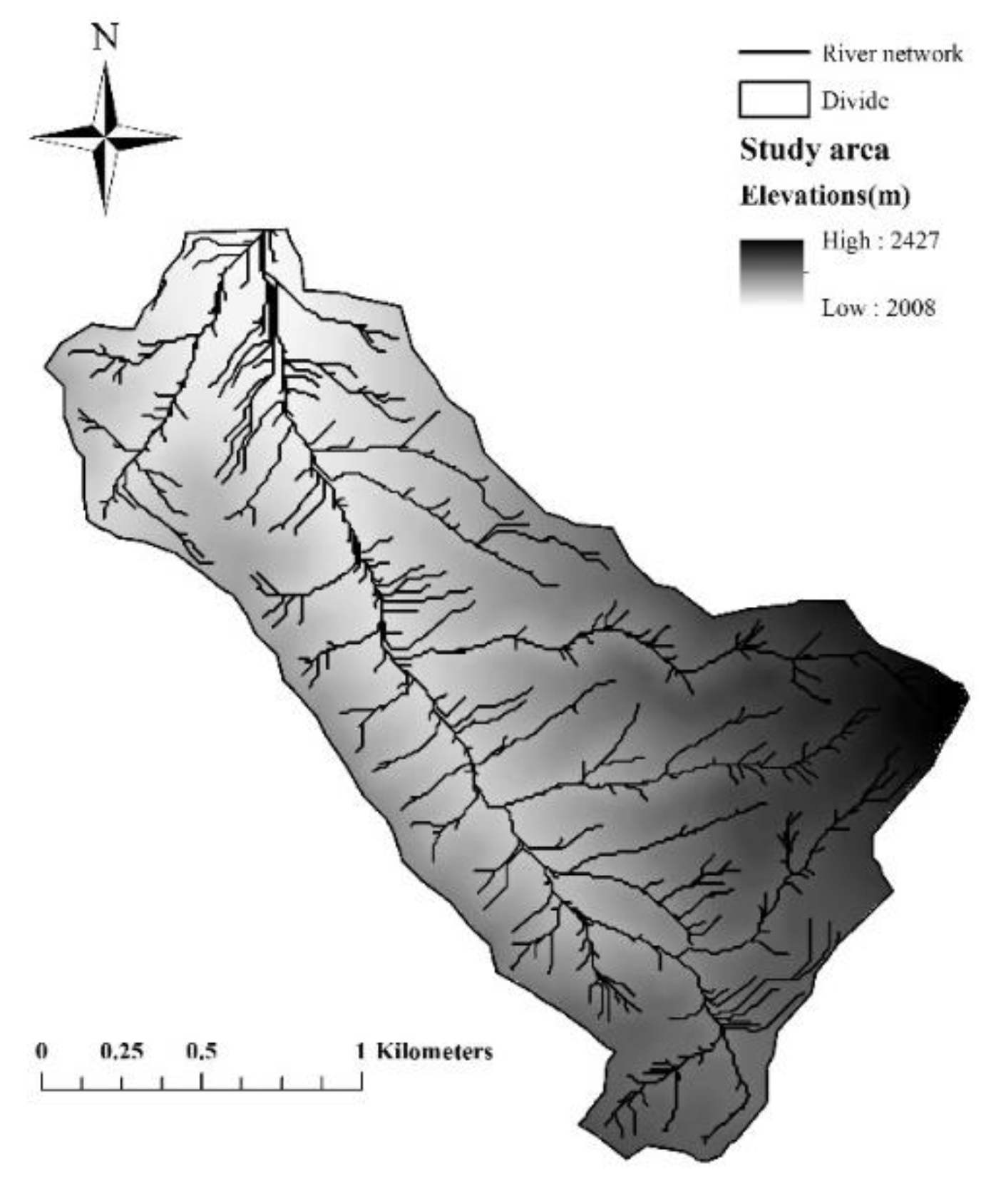
2.1. Study Area
2.2. Empirical Formulas
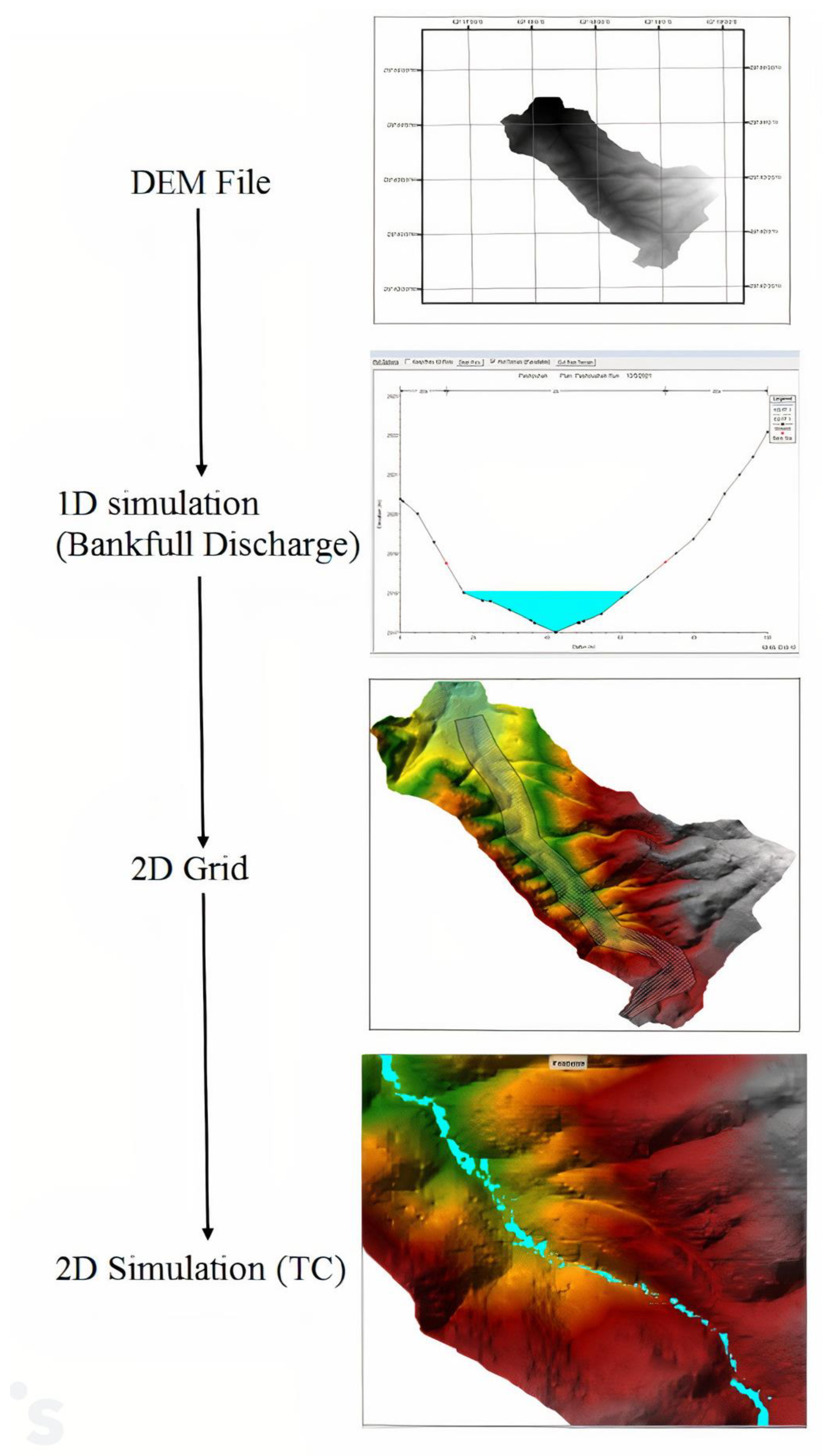
2.3. Hydraulic Simulation
3. Results and Discussions
3.1. Empirical Relations
Sensitivity Analysis Results
3.2. Hydraulic Simulation
4. Conclusions
- It is recommended to consider the graphical method (rainfall-runoff) as an alternative to salt solution tracing in a gauged basin as a benchmark to compare 2D simulation output.
- In this study, to introduce bathymetry into the model, the DEM file with a resolution of 12.5 m from the Advanced Land Observation Satellite (ALOS) was employed. It is recommended to apply higher resolution satellites or other methods such as using a drone to survey maps of the area or bathymetry with high resolution in order to investigate the map resolution effect on TC.
Author Contributions
Funding
Data Availability Statement
Acknowledgments
Conflicts of Interest
References
- Singh, V.P. Hydrologic Systems: Rainfall Runoff Modeling; Prentice Hall Publication: Bergen, NJ, USA, 1988; Volume 1, p. 960. [Google Scholar]
- McCuen, R.H. Hydrologic Analysis and Design; Prentice Hall: Englewood Cliffs, NJ, USA, 1989. [Google Scholar]
- Wong, T.S.W. Evolution of kinematic wave time of concentration formulas for overland flow. J. Hydrol. Eng. 2009, 14, 739–744. [Google Scholar] [CrossRef]
- Kirpich, Z.P. Time of concentration of small agricultural watersheds. Civ. Eng. 1940, 10, 362. [Google Scholar]
- Calkins, D.; Dunne, T. A salt tracing method for measuring channel velocities in small mountain streams. J. Hydrol. 1970, 11, 379–392. [Google Scholar] [CrossRef]
- DeAlmeida, I.K.; Almeida, A.K.; Garcia, G.S.; Alves, S.T. Performance of methods for estimating the time of concentration in a watershed of a tropical region. Hydrol. Sci. J. 2017, 62, 2406–2414. [Google Scholar] [CrossRef]
- Grimaldi, S.; Petroselli, A.; Tauro, F.; Porfiri, M. Time of concentration: A paradox in modern hydrology. Hydrol. Sci. J. 2012, 57, 217–228. [Google Scholar] [CrossRef] [Green Version]
- Ravazzani GBoscarello LCislaghi AMancini, M. Review of Time-of Concentration Equations and a New Proposal in Italy. J. Hydrol. Eng. 2019, 24, 4019039. [Google Scholar] [CrossRef]
- Soroush, Y.; Eslamian, M. Comparison of experimental formula and flood hydrograph analysis method for estimation of concentration time. In Proceedings of the 1st Regional Conference on Water, Islamic Azad University of Iran, Behbahan, Iran, 2006. (In Persian). [Google Scholar]
- McCuen, R.H.; Wong, S.L.; Rawls, W.J. Estimating Urban Time of Concentration. J. Hydraul. Eng. 1984, 110, 887–904. [Google Scholar] [CrossRef]
- Pilgrim, D.H. Regional methods for estimation of design floods for small to medium sized drainage basins in Australia. In Proceedings of the New Directions for Surface Water Modelling, Proceedings of an International Symposium 3Rd Scientific Assembly International Association Hydrological Sciences, Baltimore, Maryland, USA, 10–19 May 1989; Volume 181. [Google Scholar]
- Goitom, T.G. Evaluation of TC Methods in a Small Rural Watershed, Channel Flow and Catchment Runoff: Centennial of Manning Formula and Kuichling_ Rational Formula; Yen, B.C., Ed.; University of Virginia, U.S. National Weather Service and University of Virginia: Charlottesville, VA, USA, 1989. [Google Scholar]
- Fang, X.; Thompson, D.; Cleveland, T.G.; Pradhan, P.; Malla, R. Time of Concentration Estimated Using Watershed Parameters Determined by Automated and Manual Methods. J. Irrig. Drain. Eng. 2008, 134, 202–211. [Google Scholar] [CrossRef]
- Eslamian, S.; Mohebbi, A. Determining experimental relationships to estimate the time of concentration in mountainous watersheds. Agric. Sci. Nat. Resour. 2005, 12, 36–45. [Google Scholar]
- Dastourani, M.T.; Abdollahvand, A.; Osareh, H.; Talebi, A.; Moghaddamnia, A. Determination of application of some experimental relations of concentration time for estimation ofsurveying time in waterway. J. Watershed Manag. Res. 2011, 99, 42–52. [Google Scholar]
- González-Álvarez, Á.; Molina-Pérez, J.; Meza-Zúñiga, B.; Viloria-Marimón, O.M.; Tesfagiorgis, K.; Mouthón-Bello, J.A. Assessing the Performance of Different Time of Concentration Equations in Urban Ungauged Watersheds: Case Study of Cartagena de Indias, Colombia. Hydrology 2020, 7, 47. [Google Scholar] [CrossRef]
- Bennis., S.; Crobbedu, E. New Runoff Simulation Model for Small Urban Catchments. J. Hydrol. Eng. 2007, 12, 540–544. [Google Scholar] [CrossRef]
- Sadatinejad, S.J.; Heydari, M.A.; Honarbakhsh, A.; Abdollahi, K.; Mozdianfard, M.R. Modelling of concentration time in north Karoon River basin in Iran. World Appl. Sci. J. 2012, 17, 194–204. [Google Scholar]
- Dingman, S.L. Water in soils: Infiltration and redistribution. Phys. Hydrol. 2002, 222–242. [Google Scholar]
- Gericke, O.J.; Smithers, J.C. Review of methods used to estimate catchment response time for the purpose of peak discharge estimation. Hydrol. Sci. J. 2014, 59, 1935–1971. [Google Scholar] [CrossRef]
- Azizian, A. Uncertainty Analysis of Time of Concentration Equations based on First-Order-Analysis (FOA) Method. Am. J. Eng. Appl. Sci. 2018, 11, 327–341. [Google Scholar] [CrossRef]
- Mirzayi, S.R. Comparing experimental methods and analyzing flood hydrograph in estimating time of concentration, case study. Watershed Eng. Manag. 2014, 6, 407–414. [Google Scholar]
- Mockus, V. Watershed lag. U.S. Dept. of Agriculture, Soil Conservation Service; U.S. Dept. of Agriculture: Washington, DC, USA, 1961.
- Salimi, E.T.; Nohegar, A.; Malekian, A.; Hoseini, M.; Holisaz, A. Estimating time of concentration in large watersheds. J. Int. Soc. Poddy Water Environ. Eng. 2017, 15, 123–132. [Google Scholar] [CrossRef]
- Roussel, M.C.; Thompson, D.B.; Fang, X.; Cleveland, T.G. Time-Parameter Estimation for Applicable Texas Watersheds; Lamar University: Beaumont, TX, USA, 2005. [Google Scholar]
- Safavi, H.R. Engineering Hydrology, 3rd ed.; Arkan Danesh: Isfahan, Iran, 2011. [Google Scholar]
- Michailidi, E.M.; Antoniadi, S.; Koukouvinos, A.; Bacchi, B.; Efstratiadis, A. Timing the time of concentration: Shedding light on a paradox. Hydrol. Sci. J. 2018, 63, 721–740. [Google Scholar] [CrossRef] [Green Version]
- Mudashiru RBAbustan EBaharudin, F. Methods of Estimating Time of Concentration: A Case Study of Urban Catchment of Sungai Kerayong, Kuala Lumpur. Proc. AICCE’19 Lect. Notes Civ. Eng. 2020, 53. [Google Scholar] [CrossRef]
- Yen, B.C.; Chow, V.T. Local design storms, Vol III. Rep. H 38 No.FHWA-RD-82/065; U.S. Dept. of Transportation, Federal Highway Administration: Washington, DC, USA, 1983.
- Sharifi, S.; Hosseini, S.M. Methodology for Identifying the Best Equations for Estimating the Time of Concentration of Watersheds in a Particular Region. J. Irrig. Drain. Eng. 2011, 137, 712–719. [Google Scholar] [CrossRef] [Green Version]
- Casulli, V. A high-resolution wetting and drying algorithm for free-surface hydrodynamics. Int. J. Numer. Methods Fluids 2009, 60, 391–408. [Google Scholar] [CrossRef]
- DeJonge, K.C.; Ahmadi, M.; Ascough, J.C.; Kinzli, K.D. Sensitivity analysis of reference evapotranspiration to sensor accuracy. Comput. Electron. Agric. 2015, 110, 176–186. [Google Scholar] [CrossRef]
- Liang, L.; Li, L.; Zhang, L.; Li, J.; Li, B. Sensitivity of Penman-Monteith reference crop evapotranspiration in Tao’ er River Basin of northeastern China. Chin. Geogr. Sci. 2008, 18, 340–347. [Google Scholar] [CrossRef]
- Goyal, R.K. Sensitivity of evapotranspiration to global warming: A case study of arid zone of Rajasthan (India). Agric. Water Manag. 2004, 69, 1–11. [Google Scholar] [CrossRef]
- McKenney, M.S.; Rosenberg, N.J. Sensitivity of some potential evapotranspiration estimation methods to climate change. Agric. For. Meteorol. 1993, 64, 81–110. [Google Scholar] [CrossRef]
- Liu, C.; Zhang, D.; Liu, X.; Zhao, C. Spatial and temporal change in the potential evapotranspiration sensitivity to meteorological factors in China (1960-2007). J. Geogr. Sci. 2012, 22, 3–14. [Google Scholar] [CrossRef]
- McCuen, R.H.A. Sensitivity and Error Analysis Cf Procedures Used for Estimating Evaporation. JAWRA J. Am. Water Resour. Assoc. 1974, 10, 486–497. [Google Scholar] [CrossRef]
- Gao, Z.; He, J.; Dong, K.; Bian, X.; Li, X. Sensitivity study of reference crop evapotranspiration during growing season in the West Liao River basin, China. Theor. Appl. Climatol. 2016, 124, 865–881. [Google Scholar] [CrossRef]
- Haktanir, T.; Sezen, N. Suitability of two-parameter gamma and three-parameter beta distributions as synthetic unit hydrographs in Anatolia. Hydrol. Sci. J. 1990, 35, 167–184. [Google Scholar] [CrossRef] [Green Version]
- Simas, M.J.; Hawkins, R.H. Lag time characteristics for small watersheds in the U.S. In Proceedings of the 2nd Federal Interagency Hydrologic Modeling Conference, (HMC’ 02), Las Vegas, NV, USA, 28 July–1 August 2002. [Google Scholar]
- Li, M.; Chibber, P. Overland flow time on very flat terrains. J. Transp. Res. Board 2008, 2060, 133–140. [Google Scholar] [CrossRef] [Green Version]
- Kent, K.M. Time of Concentration; National Engineering Handbook; USA. 1972. Available online: https://directives.sc.egov.usda.gov/OpenNonWebContent.aspx?content=18389.wba (accessed on 1 August 2022).
- Perdikaris, J.; Gharabaghi, B.; Rudra, R. Reference Time of Concentration Estimation for Ungauged Catchments. Earth Sci. Res. 2018, 7, 58. [Google Scholar] [CrossRef]
- Chow, V.T. Open-Channel Hydraulics. In Ven Te Chow; McGraw-Hill: New York, NY, USA, 1959; pp. xviii + 680. [Google Scholar]


| Parameter | Value | Unit |
|---|---|---|
| Differences in main river elevation | 273 | m |
| Watershed length | 3323.2 | m |
| Watershed width | 1859.2 | m |
| mean elevation | 2217.5 | m |
| area | 3.53 | km2 |
| Main river average slope | 0.07 | m/m |
| Watershed average slope | 0.298 | m/m |
| Equivalent circle diameter | 2120.14 | m |
| CN | 76.41 | - |
| Equation Name and References | Formula | Description | Estimated TC (h) | RE (%) | ||
|---|---|---|---|---|---|---|
| Estimated by Empirical Method | 2D Simulation (Average of Two Estimations) | Equations | 2D Simulation | |||
| Haktanir and Sezen, [6,20] | Derived from 10 basins in Turkey, 11 < A < 9867 km2 | 2.132 | (1.8 + 2.22/2) = 2.01 | 22.124 | 14.85 | |
| Temez, [21] | For Spain natural watersheds | 1.303 | 25.347 | |||
| Bransby –William, [8,21] | Rural watersheds, A < 129.5 km2 | 1.284 | 26.440 | |||
| Pilgrim and McDermott, [8,21] | 0.1 < A < 250 km2 | 1.227 | 29.716 | |||
| Pasini, [21] | Italian rural watersheds | 0.948 | 45.729 | |||
| US Army Corps of Engineers, [8] | A < 0.5 km2 | 0.83 | 52.471 | |||
| Picking, [21] | Rural watersheds | 0.499 | 71.436 | |||
| Kirpich -Tennessee, [22] | 4 < A < 50 ha, S: 3 < < 10% | 0.490 | 71.912 | |||
| California Curvets Practice (CHPW), [21] | For small mountainous US watersheds | 0.474 | 72.846 | |||
| Johnston and Cross, [7] | 64 < A < 4200 km2 | 0.387 | 77.840 | |||
| Van Sickle, [10] | A < 36 sq mile | 0.229 | 86.897 | |||
| Kirpich -Pennsylvania, [21] | 0.004 < A < 0.453 km2, 0.03 < < −0.1 | 0.111 | 93.655 | |||
| Chow, [8,20] | 0.01 < A < 18.5 km2, 0.0051 < < 0.09 m/m | 0.809 | 53.7 | |||
| Flavell, [21] | 0.1 < A < 250 km2 | 4.564 | 161.379 | |||
| Carter, [10] | A < 8 sq mile, L < 8 miles, = 0.5% | 6.073 | 247.843 | |||
| Sheridan, [21] | 2.62 < A < 364.34 km2 | 7.064 | 304.606 | |||
| Equation Name | Formula | Description | TC (h) | RE (%) | ||
|---|---|---|---|---|---|---|
| Estimated by Empirical Method | 2D Simulation (Average of Two Estimations) | Equations | 2D Simulation | |||
| Simas and Hawkins, [21] | 0.001 < A < 14 km2 | 1.863 | (1.8 + 2.22/2) = 2.01 | 6.722 | 14.85 | |
| SCSlag, [23] | A < 8 km2 | 1.592 | 8.660 | |||
| Williams, [6] | India Watersheds, A < 129.5 km2 | 1.285 | 26.398 | |||
| TXDOT, [24,25] | A < 0.8 km2 | 0.752 | 56.956 | |||
| Equation Name | Formula | Description | Estimated TC (h) | RE (%) | ||
|---|---|---|---|---|---|---|
| Estimated by Empirical Method | 2D Simulation (Average of Two Estimations) | Equations | 2D Simulation | |||
| Kadoya and Fukushima, [26,27] | km2 < 143 A < 0.5 | 1.321 | (1.8 + 2.22/2) = 2.01 | 24.335 | 14.85 | |
| Morgali and Linsley, [26,27,28] | small catchment, urban areas, A < 10 to 12 ha | 1.149 | 34.169 | |||
| Arizona DOT, [21] | Agricultural watersheds | 0.948 | 45.707 | |||
| US Army, [26,27] | Derived from concrete trough, A = 500 ft, S = 0.5, 1 and 2 % | 0.478 | 72.634 | |||
| Equation Name | Formula | Description | Estimated TC (h) | RE (%) | ||
|---|---|---|---|---|---|---|
| Estimated by Empirical Method | 2D Simulation (Average of two Estimations) | Equations | 2D Simulation | |||
| Bransby–William, [8,21] | Rural watersheds, A < 129.5 km2 | 1.262 | (1.8 + 2.22/2) = 2.01 | 27.708 | 14.85 | |
| Ventura, [8,21] | rural watersheds, A < 10 km2 | 0.857 | 50.899 | |||
| Pickerin, [21] | Equivalent to Kirpich | 0.473 | 72.898 | |||
| Basso, [21] | Wave equation and green-ampt infiltration method | 0.213 | 27.708 | |||
| Equation Name | Formula | Description | Estimated TC (h) | RE (%) | ||
|---|---|---|---|---|---|---|
| Estimated by Empirical method | 2D Simulation (Average of Two Estimations) | Equations | 2D Simulation | |||
| Yen and Chow’s, [29] | overland flow, A < 50 km2 | 1.510 | (1.8 + 2.22/2) = 2.01 | 13.515 | 14.85 | |
| NRCS, [7,8] | Small rural basins, sA < 8 km2 | 1.435 | 17.818 | |||
| Hathaway, [21,30] | Analysis of overland flow, L < 0.37 km, A < 10 ha | 1.067 | 38.882 | |||
| Equation | SL | SSr | SLt | SA |
|---|---|---|---|---|
| Kirpich-Pennsylvania | 0.772 | −0.522 | - | - |
| Kirpich-Tennessee | 0.772 | −0.400 | - | - |
| Chow | 0.644 | −0.332 | - | - |
| Espey | 0.364 | −0.185 | - | - |
| US Corps of Engineers | 0.763 | −0.196 | - | - |
| Temez | 0.763 | −0.196 | - | - |
| Carter | 0.604 | −0.311 | - | - |
| Johnston and Cross | 0.504 | −0.522 | - | - |
| Picking | 0.670 | −0.345 | - | - |
| Haktanir and Sezen | 0.843 | - | - | - |
| Sheridan | 0.921 | - | - | - |
| Van Sickle | 0.132 | −0.067 | 0.132 | - |
| Bransby –William | 1.000 | −0.206 | - | −0.103 |
| Pasini | 0.337 | −0.522 | - | 0.337 |
| California Curvets Practice (CHPW) | 1.153 | - | - | - |
| Flavel | - | - | - | 0.544 |
| Pilgrim and Mac Dermott | - | - | - | 0.384 |
| Equation | SL | SSr | SSb | SD | SA | SCN | Sc | Slag |
|---|---|---|---|---|---|---|---|---|
| William | 1.000 | - | −0.206 | −1.072 | 0.404 | - | - | - |
| Bransby Williams | 1.000 | - | −0.206 | −1.072 | 0.404 | - | - | - |
| SCSlag | 0.802 | −0.522 | - | - | - | −2.357 | - | - |
| Simas and Hawkins | −0.623 | −0.154 | - | - | 0.598 | −1.613 | - | - |
| Kerby | 0.474 | - | −0.243 | - | - | - | - | 0.474 |
| TXDOT | 0.504 | - | −0.345 | - | - | - | −0.528 | - |
| Equation | SL | SSr | Sn | SA | Slca | SP24 |
|---|---|---|---|---|---|---|
| Arizona DOT | 0.254 | −0.206 | - | - | 0.254 | 0.102 |
| US Army Corps of Engineers | 0.540 | −0.076 | - | - | - | −0.448 |
| Morgali and Linsley | 0.604 | −0.311 | 0.604 | - | - | −0.416 |
| Kadoya and Fukushim | - | - | - | 0.224 | - | −0.363 |
| Equation | SL | SH | SA | SE |
|---|---|---|---|---|
| Bransby–William | 1.198 | −0.206 | −0.103 | - |
| Ventura | 0.504 | −0.522 | 0.504 | - |
| Pickerin | 1.153 | −0.400 | - | - |
| Basso | 1.153 | - | - | −0.400 |
| Equation | SL | SSr | SSb | Sn | Si |
|---|---|---|---|---|---|
| Yen and Chow’s | 0.604 | −0.522 | - | 0.604 | - |
| Hathaway | 1.000 | - | −0.522 | 1.000 | - |
| NRCS | - | −0.361 | −0.078 | 0.150 | −0.098 |
| Simulation Discharge (m3/s) | Estimated TC (h) | RE (%) |
|---|---|---|
| Qb(max) | 1.8 | 3.1 |
| Qb(min) | 2.22 | 26.98 |
Publisher’s Note: MDPI stays neutral with regard to jurisdictional claims in published maps and institutional affiliations. |
© 2022 by the authors. Licensee MDPI, Basel, Switzerland. This article is an open access article distributed under the terms and conditions of the Creative Commons Attribution (CC BY) license (https://creativecommons.org/licenses/by/4.0/).
Share and Cite
Zolghadr, M.; Rafiee, M.R.; Esmaeilmanesh, F.; Fathi, A.; Tripathi, R.P.; Rathnayake, U.; Gunakala, S.R.; Azamathulla, H.M. Computation of Time of Concentration Based on Two-Dimensional Hydraulic Simulation. Water 2022, 14, 3155. https://doi.org/10.3390/w14193155
Zolghadr M, Rafiee MR, Esmaeilmanesh F, Fathi A, Tripathi RP, Rathnayake U, Gunakala SR, Azamathulla HM. Computation of Time of Concentration Based on Two-Dimensional Hydraulic Simulation. Water. 2022; 14(19):3155. https://doi.org/10.3390/w14193155
Chicago/Turabian StyleZolghadr, Masih, Mohamad R. Rafiee, Fatemeh Esmaeilmanesh, Abazar Fathi, Ravi Prakash Tripathi, Upaka Rathnayake, Sreedhar Rao Gunakala, and Hazi Mohammad Azamathulla. 2022. "Computation of Time of Concentration Based on Two-Dimensional Hydraulic Simulation" Water 14, no. 19: 3155. https://doi.org/10.3390/w14193155