Article

Investigating Machine Learning Applications for Effective Real-Time Water Quality Parameter Monitoring in Full-Scale Wastewater Treatment Plants

UnU Inc., Samsung IT Valley, 27, Digital-ro 33-gil, Guro-gu, Seoul 08380, Korea
*
Authors to whom correspondence should be addressed.
Water 2022, 14(19), 3147; https://doi.org/10.3390/w14193147
Submission received: 19 August 2022 / Revised: 19 September 2022 / Accepted: 4 October 2022 / Published: 6 October 2022
(This article belongs to the Special Issue AI and Deep Learning Applications for Water Management)

Abstract

:
Environmental sensors are utilized to collect real-time data that can be viewed and interpreted using a visual format supported by a server. Machine learning (ML) methods, on the other hand, are excellent in statistically evaluating complicated nonlinear systems to assist in modeling and prediction. Moreover, it is important to implement precise online monitoring of complex nonlinear wastewater treatment plants to increase stability. Thus, in this study, a novel modeling approach based on ML methods is suggested that can predict the effluent concentration of total nitrogen (TNeff) a few hours ahead. The method consists of different ML algorithms in the training stage, and the best selected models are concatenated in the prediction stage. Recursive feature elimination is utilized to reduce overfitting and the curse of dimensionality by finding and eliminating irrelevant features and identifying the optimal subset of features. Performance indicators suggested that the multi-attention-based recurrent neural network and partial least squares had the highest accurate prediction performance, representing a 41% improvement over other ML methods. Then, the proposed method was assessed to predict the effluent concentration with multistep prediction horizons. It predicted 1-h ahead TNeff with a 98.1% accuracy rate, whereas 3-h ahead effluent TN was predicted with a 96.3% accuracy rate.

1. Introduction

Wastewater treatment plants (WWTPs) are an integral part of urban water infrastructure for minimizing pollutants and preserving public health. Effluent quality, energy consumption, and resource recycling restrictions for WWTPs are becoming more stringent [1,2]. Increasingly, mathematical models are utilized to quantify the effectiveness of WWTPs and to build optimum operating strategies by establishing a quantitative link between influent WWTP features and effluent water quality [3]. Furthermore, nitrogen is a major contaminant in wastewater that must be reduced to a specified level prior to wastewater discharge. Ammonia, nitrite, nitrate, and organically bound nitrogen are the principal types of total nitrogen (TN) in wastewater [4]. Monitoring TN in the influent of WWTPs is essential for the performance of nutrient removal systems, the control of sludge production, and the operation of different wastewater treatment processes [5].
Engineers must grasp and quantify wastewater properties, especially nutrient components, at the start and end of treatment. To obtain the necessary data, the operator must collect sensor data or sample wastewater and analyze the plant’s influent/effluent flow to identify the characteristics of the raw waste. The entry of improperly treated wastewater, one of the sources of nutrients, into water bodies such as groundwater systems may result in several health issues [6]. However, many WWTPs have upgraded their facilities to increase the removal of nutrient pollutants, resulting in a substantial decrease in the quantity of nutrients discharged by WWTPs [7]. Most artificial intelligence (AI) methods are used to predict natural or artificial processes in a range of areas. As a subset of AI, machine learning (ML) is the process of identifying a pattern in data for the purpose of prediction or classification [8]. In recent years, the modeling and forecasting of environmental phenomena using AI technology have surged because of its capability to solve practical problems related to sewage treatment [9], river quality monitoring [10], and management of water resources [11]. In their study, Bagheri et al. [12] investigated the impact of AI models on the prediction and assessment of leachate penetration from a landfill site into groundwater. These algorithms may unearth more intricate links than statistical methods [13,14]. Water quality prediction may benefit from the use of neural network methods [15]; however, the issue of inadequate training should not be overlooked [16]. Furthermore, a hybrid model was designed to increase the accuracy of water quality prediction; however, the model was unable to learn the state features across time series data, which might result in high mistakes in extreme value prediction [17].
In addition, deep learning (DL) algorithms have become the most popular data-driven modeling algorithms in recent years because of their potent nonlinear mapping and learning capabilities. The applications of DL methods were critically reviewed for better control and management of membrane fouling in wastewater treatment systems [18]. Ma et al. [19] utilized DL to forecast the 5-day biological oxygen demand (BOD5) of New York harbor water and produced an R2 value that was 22–40% of the other six standard data-driven models assessed. Recurrent neural networks (RNNs) are also utilized for water quality prediction because of their incorporated feedback and recursive structure, which enables them to maintain information from earlier times and use prior information to predict present information [20]. Jiang et al. [21] developed five data-driven models to forecast the high-cost indicators of sewage in drainage networks; the accuracy of multiple linear regression (MLR) was only 70–75% of the long short-term memory (LSTM) neural network. Previous research has demonstrated that the LSTM model is more accurate and suited for time series data prediction than standard neural network models [22,23]. Furthermore, attention-based RNNs can now dynamically learn spatiotemporal associations and obtain the greatest results in single-step prediction of multivariate time series [24]. Using RNN methods as a modeling algorithm is an efficient method for enhancing the precision of modeling-based water quality detection.
In contrast, feature selection is utilized in the preprocessing step to increase training time, enhance prediction accuracy, and simplify models [25]. In this study, we employ a strategy based on recursive feature elimination (RFE) to eliminate irrelevant features. Dey and Rahman [26] showed that RFE is beneficial for correlated predictors in general. For water quality, many of the physiochemical characteristics are not independent of one another; hence, RFE is believed to be effective for enhancing prediction models for wastewater quality metrics. There are two primary objectives to accomplish during feature selection: (1) One may like to identify all significant factors associated with the outcome variable, or (2) one may wish to find a minimum collection of variables that provides a decent prediction model that is not overfitted and can generalize to other datasets. Regarding the forecast of water quality parameters, the second objective will be the most essential.
We observed in the literature that many models were constructed without the identification of predictive elements. Consideration of all characteristics for prediction may provide an insufficient starting point for estimating water quality and may not adequately represent effluent variance [27]. Therefore, the utilization of all indicators without a better selection of predictive ones may not improve the sensitivity of wastewater effluent fluctuation. A selection of predictive transactional characteristics is crucial for constructing an efficient model for predicting water quality. To have a relevant selection of characteristics for the researched model, it is required to have access to many real-time databases, which is essential for achieving an accurate assessment performance.
This research proposes a unique hybrid paradigm for predicting the changing effluent loads of WWTPs with complicated processes. In this regard, the contribution of this study is the development of a specialized multistep prediction model based on ML and RNN algorithms that can maintain predictive capability at different time horizons by addressing the highly nonlinear characteristics of the influent and effluent dataset in the presence and absence of sensors. This study’s novelties include: (1) The data preprocessing step combines the hourly recorded time series sensor and operating parameters, applies min–max normalization, and generates time shift data; (2) The feature selection phase finds the relevant features by using wrapper feature selection. The wrapper-based RFE selects the optimal features using decision tree as the feature evaluator and finds the optimal subset of features for high predictive ability; (3) The deep prediction phase predicts the future effluent TN by using predictive models, including partial least squares (PLS), MLR, multilayer perceptron (MLP), LSTM, gated recurrent unit (GRU), and multihead-attention-based GRU (MAGRU). The performance of the predictive models is conducted to select the best models and determine the multistep sequence prediction of the effluent TN. The proposed innovative framework showed a greater capacity for prediction by virtue of its ML and RNN architectures. To verify the applicability of the proposed prediction methodology for directing the short- and long-term operational strategies of WWTPs, it was applied to multistep (1 h and 3 h ahead) prediction horizons over a case study, a WWTP in South Korea. The outcome of this study is highly beneficial to industrialists and policymakers when devising proactive decisions for enhanced wastewater treatment management.

2. Materials and Methods

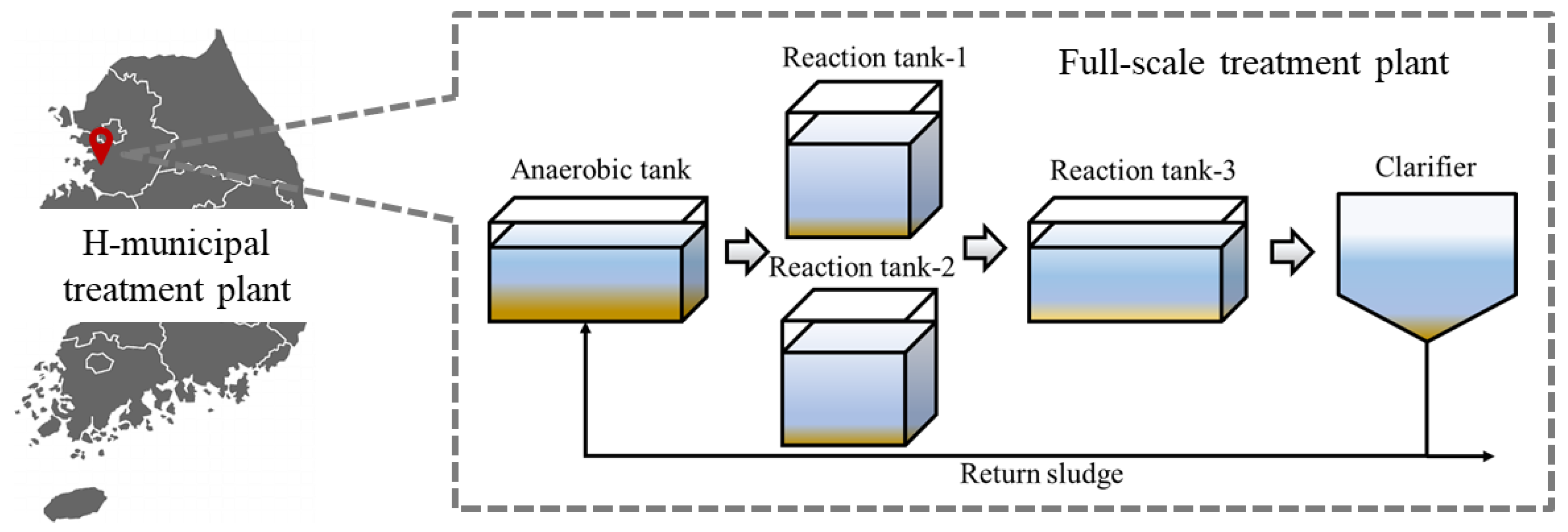
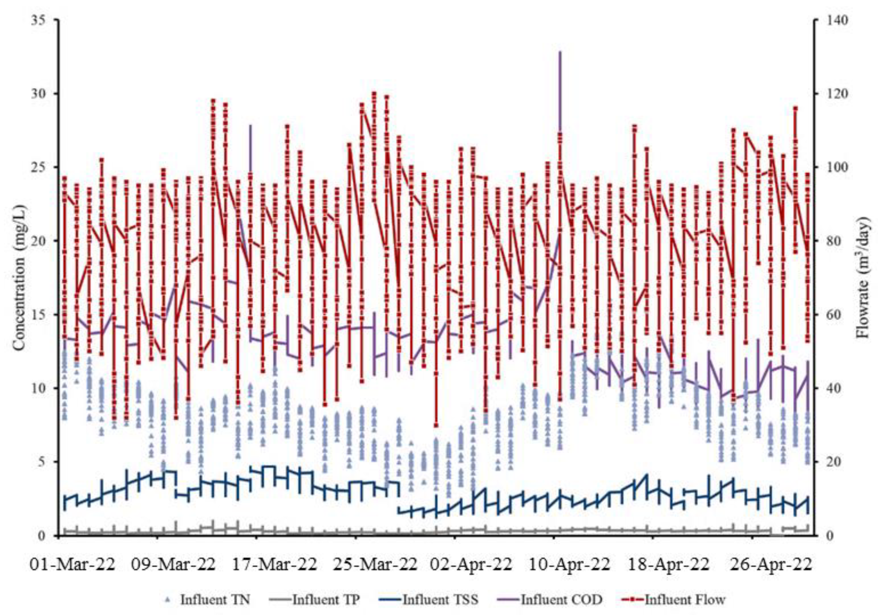
2.1. Target WWTP and Online Data Analysis

This study examined a data set from the H-municipal treatment plant for nutrient removal, which is situated in South Korea. This WWTP is built for a mean capacity of 22,000 tons/day. The WWTP has a sedimentation tank, anaerobic/aerobic reactors, and a clarifier. As shown in Figure 1, the WWTP consisted of pretreatment, a grit chamber, and an activated sludge system, which included anaerobic, anoxic, and aerobic tanks. The biological treatment system was followed by a secondary clarifier and then treated with flocculation, sedimentation, sand filtration, and disinfection before discharge as the final effluent.
A training set of data consisting of hourly measurements of total nitrogen (TN), total suspended solids (TSS), biological oxygen demand (BOD), chemical oxygen demand (COD), mixed liquor suspended solids (MLSS), total phosphorus (TP), influent flowrate (Qin), effluent flowrate (Qeff), return flowrate (RAS), waste flowrate (WAS), and dissolved oxygen (DO). The statistics of WWTP influent and effluent waste quality data are shown in Table 1. The mean influent COD, MLSS, TSS, TN, and TP were 13.06 mg/L, 2892.07 mg/L, 2.76 mg/L, 8.13 mg/L, and 0.35 mg/L, respectively. In addition, two months (1 March 2022–30 April 2022) hourly dataset were chosen for a dynamic-state model testing and prediction, which is shown in Figure 2. The operation data were collected in real time, with a data collection frequency of 1 h. Furthermore, to produce an appropriate model, the dataset must be standardized, and unnecessary datasets must be removed to prevent overfitting. One of the primary objectives of this research is to assess the impact of relevant parameters on model accuracy with or without sensor data.

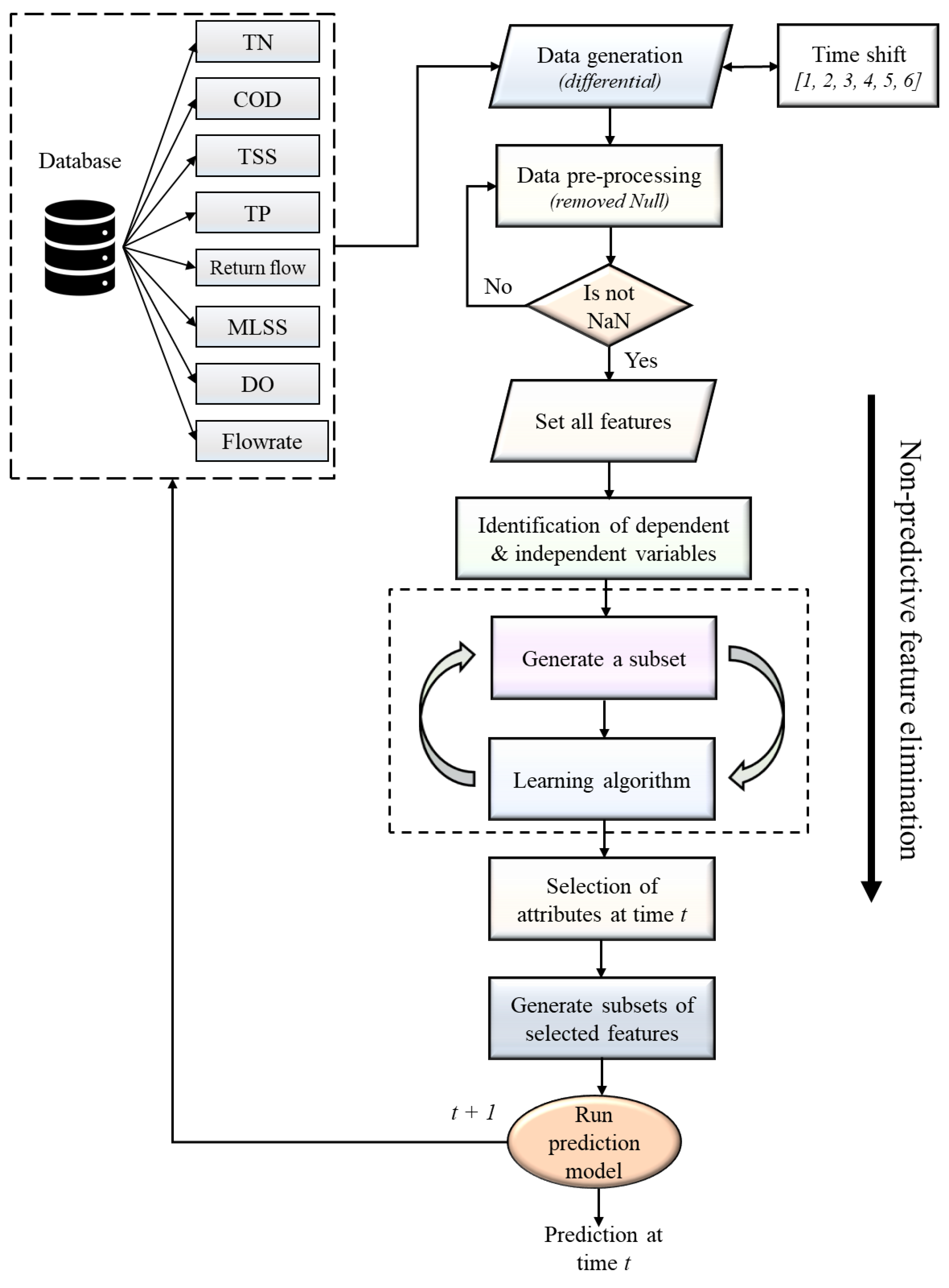
2.2. Selection of Predictive Features

The main goal of feature selection is to obtain the most relevant sensor and operating parameters from a dataset. Reducing the number of features utilized before training an ML model may increase its runtime and efficiency [28]. In practice, feature reduction is difficult and often needs lengthy testing. In the ML field, there are several strategies for selecting predictive features, a set of features that effectively predicts the likelihood of an outcome, or nonpredictive features [29].
Recursive feature elimination is a procedure that eliminates nonpredictive features without increasing the model’s error, hence accelerating learning and minimizing training time. Therefore, the most useful data with predictive capabilities are crucial. Nkiama et al. [30] used an RFE approach coupled with a decision-tree-based classifier to extract pertinent characteristics for the goal of enhancing a detection system. The study offers credence to the notion that feature selection based on RFE may be utilized to enhance classifier performance and identify significant features of influent and effluent water quality parameters. Figure 3 depicts the RFE method of removing nonpredictive characteristics implemented in this study. This represents the procedure for data generation, directly taken from the SCADA database, preprocessing, and elimination of water parameters using RFE with a decision tree model as the eliminator. At each time step t feature selection, the effluent TN at t is predicted, and the operation is repeated until completion.

2.3. Prediction Models for Water Quality Parameter

In this section, we describe several prediction models based on machine learning, artificial neural network, and recurrent neural network, which we used in our study. Additionally, the internal process of the Transformer model with multihead attention mechanisms is presented in this section.

2.3.1. Partial Least Squares (PLS) Model

The partial least squares (PLS) technique is a mature method. It produces orthogonal components by applying existing correlations between explanatory variables and corresponding outputs. The PLS model can be represented in matrix form as Equation (1) [31].
Y = X × C + R
where C is the regression coefficients matrix, and R is the residuals matrix.

2.3.2. Stepwise Multiple Linear Regression (MLR) Model

MLR was used to establish the pattern of relationships between predictors and outcome variables. In general, the model can be written as Equation (2) [32].
Y = B o = B 1 X 1 = B 2 X 2 + + B k X k + ε
where Y is the dependent variable, X 1 , X 2 ,… X k are the predictor variables, and ε is the error term.

2.3.3. Multilayer Perceptron (MLP) Model

MLP is a parameter-free modeling technique used to estimate a function between inputs and outputs. As illustrated in Figure 4, it comprises three layers: input, hidden, and output. Backpropagation is used to continuously change the network’s weights to decrease the error rate throughout the MLP learning process. Backpropagation computes the gradient of the weight space with respect to error computed by a loss function and updates the network’s weights using stochastic gradient descent and other techniques [33].

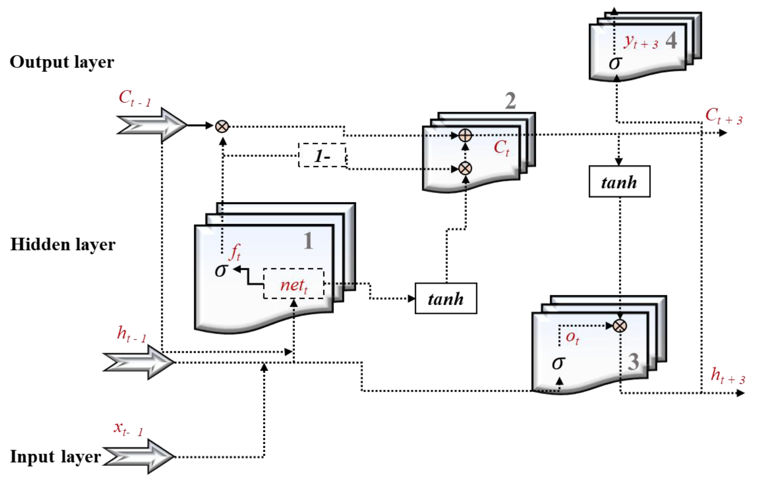
2.3.4. Memory Gated Recurrent Neural Networks

In this section, RNN versions of recurrent units (i.e., LSTM and GRU) were created. In this work, we compared RNN architectures, namely, LSTM and GRU. Multiple hidden recurrent layers are piled above one another in RNNs. The output of one recurrent layer serves as the input for the subsequent layer.
The depth of LSTM architecture determines the important forget gate f t , whereas the input gate x t updates the additions using the term of candidates C t , and then the output gate y t generates the prediction values, as given in Equations (3)–(6) [34].
f t = σ × ( w f × [ h t 1 , o t ] + b f )
x t = σ × ( w i × [ h t 1 , o t ] + b x )
C t = tanh ( w C × [ h t 1 , o t ] + b c )
y t = σ ( w o [ h t 1 , o t ] + b o )
where σ ( ) is the activation function, w is the weight of the matrices, b is the bias vector of the function, h t 1 is the output value at time t − 1, and x t is the input at time t. The schematic representation of the LSTM is shown in Figure 5. The GRU structures are described using Equations (7)–(10) [35].
z t = σ ( w z [ h t 1 , x t ] )
r t = σ ( w t [ h t 1 , x t ] )
h ~ t = tanh ( w C [ r t h t 1 , x t ] )
h t = ( 1 z t ) h t 1 + z t h ~ t
where h ~ t is the current candidate produced by z t and r t at time t, and h t is the activate function to define the final output at time t.

2.3.5. Transformer Multihead Attention Network

Google team’s suggested Transformer is a traditional natural language processing solution that is superior to RNNs for machine translation jobs [36]. This model depends primarily on an attention mechanism and has the capacity to be parallelized successfully, as assessed by the minimal number of consecutive operations necessary. Transformer avoids the RNN model restriction that important computations cannot be conducted in parallel, and the number of operations necessary to determine the relationship between two points does not grow with distance [37]. Transformer construction is shown in Figure 6; the model comprises stacked encoders and decoders with multihead attention and time-scattered layers.
Inspired by the visual attention mechanism of the fovea, a selective attention mechanism concentrating on the important bits of the input has been suggested by assessing the output’s sensitivity to the variance of the input [38]. This kind of attention strategy not only fundamentally increases model performance, but also facilitates enhanced interpretability, as described using the following equations.
α i = softmax ( f ( k e y i , q ) )
a t t ( ( K , V ) , q ) = α i = 1 N × α i × X i
a t t e n t i o n ( ( K , V ) , Q ) = a t t ( ( K , V ) , q 1 ) a t t ( ( K , V ) , q M )
An attention function can be described as mapping a query and a set of key–value pairs to an output, where the query, keys, values, and output are all vectors. The output is computed as a weighted sum of the values, where the weight assigned to each value is computed by a compatibility function of the query with the corresponding key. Multihead attention allows the model to jointly attend to information from different representation subspaces at different positions, as given in Equation (14).
M u l t i H e a d ( Q , K , V ) = C o n c a t ( h e a d 1 , h e a d h ) × W o w h e r e , h e a d i = A t t e n t i o n ( Q × W i Q , K × W i K , V × W i V )
where the projections are parameters matrices W i Q d model , W i K d model × d k , W i V d model × d v and W o h d v × d model . In this work, we employed h = 2 parallel attention layers or heads. For each of these, we use dk = dv = 32 and dmodel = 50.

2.4. Performance Evaluation

Using four performance metrics, the predictive prediction method’s efficacy was tested. These include the root mean squared error (RMSE), the mean absolute error (MAE), the coefficient of determination (R2), and the mean square error (MSE). These metrics are provided below:
R M S E = i = 1 n ( y ^ i y i ) 2 n 1
M A E = 1 n × i = 1 n | y ^ i y i |
R 2 = 1 i = 1 n ( y ^ i y i ) 2 i = 1 n ( y i y ¯ ) 2
M S E = i = 1 n ( y i y ^ i ) 2 n
where n represents the number of test observations, y ^ i is the predicted data, and y i is the experimental data. A lower value of the error metrics, and a higher R2 value represent higher accuracy and prediction performance.

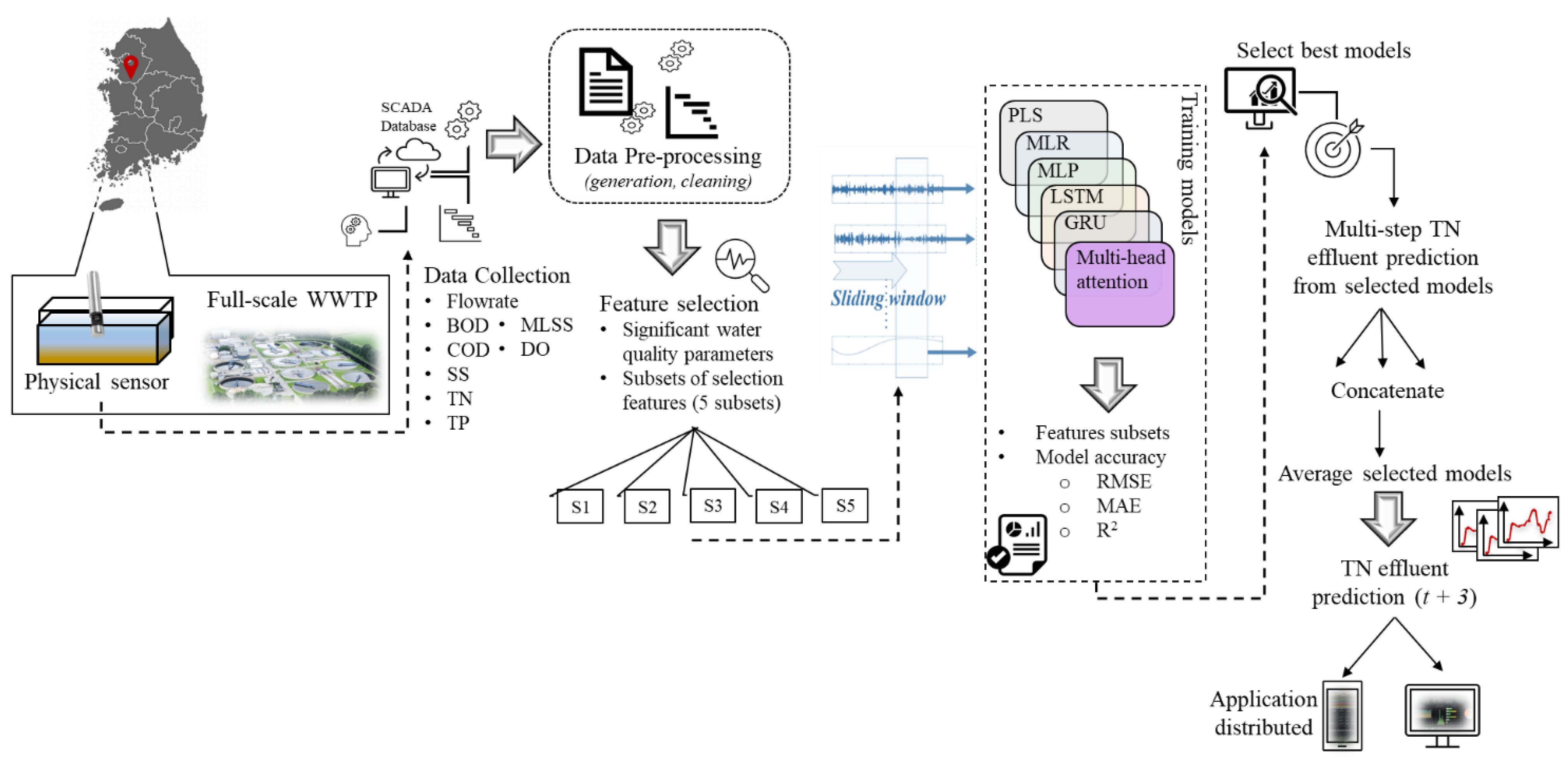
2.5. Proposed Multistep Ahead TN Prediction Methodology

Figure 7 presents a proposed framework for a multistep ahead effluent TN prediction at WWTPs under dynamic variational data. The proposed framework is divided into four main stages: (1) Data preprocessing and data generation, (2) feature selection by recursive feature elimination (RFE) method, (3) sliding windows analysis and training of various machine learning and deep learning models, and (4) multistep (t + 1 and t + 3) effluent TN prediction based on selected best models. In this study, the effluent TN prediction model was developed for hourly sequence prediction horizons. In the first stage, the hourly recorded sensor and reactor dataset of the full-scale WWTP was collected. Then, it was cleaned and normalized to prepare the suitable data for further processing and generate the hourly time shift data of the sensor and reactors. In the second stage, a recursive feature elimination method, wrapper feature selection, was applied to identify the significant and relevant features, as explained in Section 2.2. RFE searches for a subset of attributes, starting with all features and removing attributes according to a score, until reaching the number of attributes to use and producing the optimal subset of features. The RFE selects both sensor data, such as COD, BOD, SS, and TP, and operating parameters, including flowrate, MLSS, and DO, if all sensors are working well. Otherwise, it selects the features from reactor data when the sensor is malfunctioning.
In the third stage, the moving window concept was configured by selecting one hour past observation to identify the complex patterns in the neighborhood data, and future data points were predicted. Then, multiple sequence predictions were conducted by using several ML and RNN models, including PLS, MLR, MLP, LSTM, GRU, and MAGRU. The prediction models were developed and trained with the selected features and subsets of RFE. Then, the parameters of the constructed models were tuned by using the time series cross-validation on a rolling basis with validation data. Finally, the performance of the trained models with selected features was compared by employing the metrics mentioned in Section 2.4. In the fourth stage, the best models were selected from the above-mentioned models each trained using a different machine learning method. The criteria for selection as the best model are the MAE of each model obtained during evaluation after feature selection. The model with the highest MAE score was chosen as the best model. Then, prediction from selected models with optimal subsets was conducted, and the prediction values were concatenated to handle the influent and effluent characteristics of wastewater treatment plants. It can boost the model performance and capture significant information in the temporal pattern of effluent TN. Then, an average was made of all predicted models. Finally, multistep prediction of effluent TN may exhibit more reliable and superior results for highly nonlinear and nonstationary effluent parameters in various prediction horizons.
Computationally, the proposed multistep ahead TN prediction implementation was conducted through PyCharm IDE with the following features: Intel® Core (TM) i7-11700 @ 2.50 GHz, 32.0 GB RAM, x64-based processor.

3. Results and Discussions

Our primary objective is to comprehend the capability of ML and AI models for predicting the WWTP’s future condition hours ahead of time. We also investigated how various factors impact the quality of the prediction.

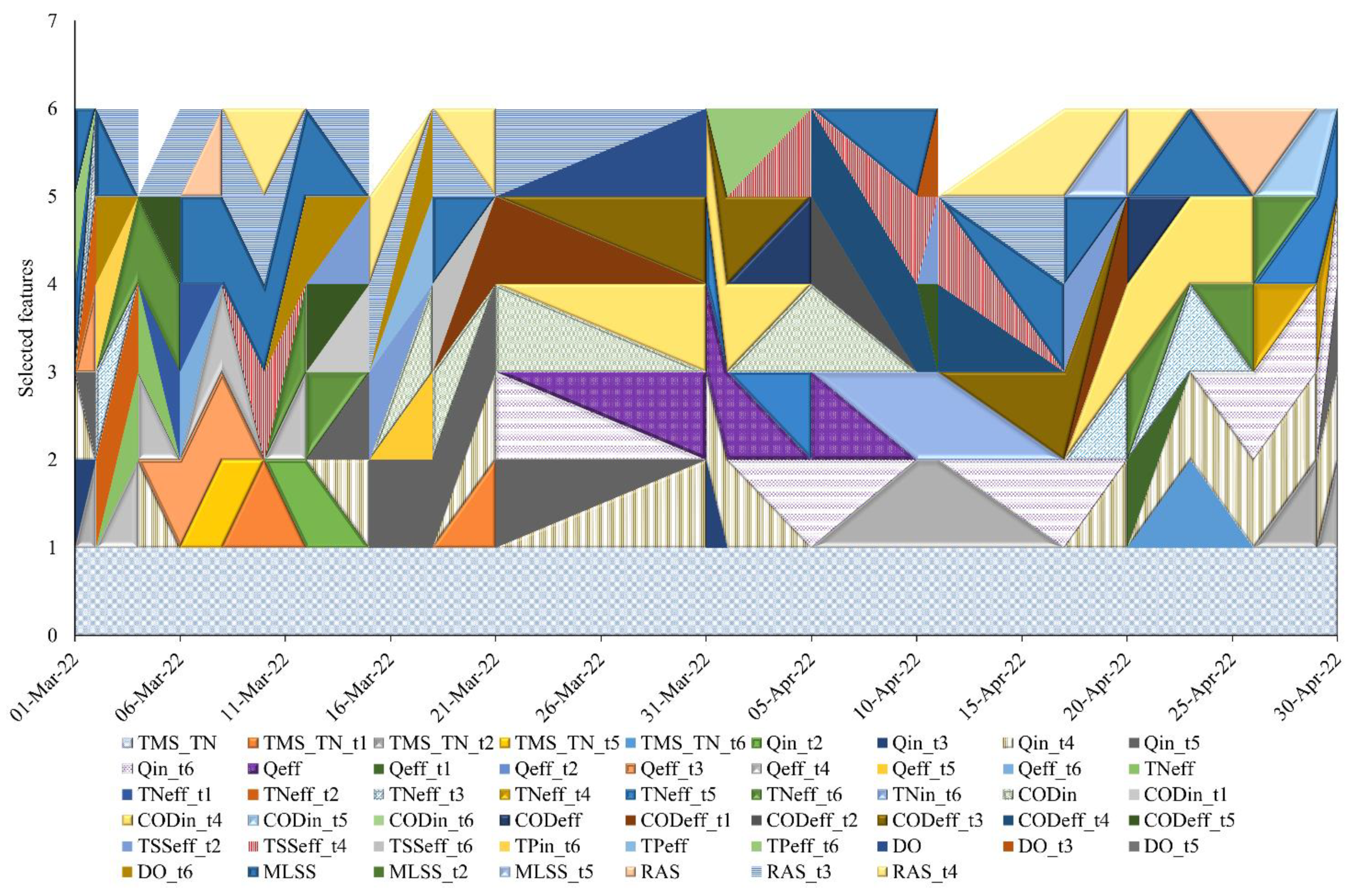
3.1. Selection of Significant Features for Effluent TN Prediction

A wastewater treatment system is a complicated system influenced by several variables. The primary process parameters in the treatment process are critical for the stable and efficient operation of WWTPs, and the inclusion of process parameters (DO in the aerobic zone, DO in the anoxic zone, MLSS) may not only increase prediction accuracy, but also give support for future model application. We conducted a study utilizing RFE with decision tree and cross-validation to identify the appropriate number of features for evaluating the most important water characteristics. These characteristics (water parameters) were then graded according to their impact on the classification accuracy of each model. The feature selection was implemented as described in Section 2.2.
After preliminary screening, 52 variables are selected as the input of the RFE which includes four influent parameters recorded using a physical sensor (CODin, TPin, TSSin, and TNin,), four effluent parameters (CODeff, TPeff, TSSeff, and TNeff), and reactor parameters (TMS_TN, DO, MLSS, and WAS, RAS, Qin, and Qeff). The top six dependent variables were selected at current time step t. Figure 8 illustrated the selection of water parameters in time series for the period of two months. The patterns represent the sensor, reactors, influent, and effluent parameters, where TMS-TN was selected at each time step t. The subsets of five of the selected parameters were taken for the training models, which are described in the following section.

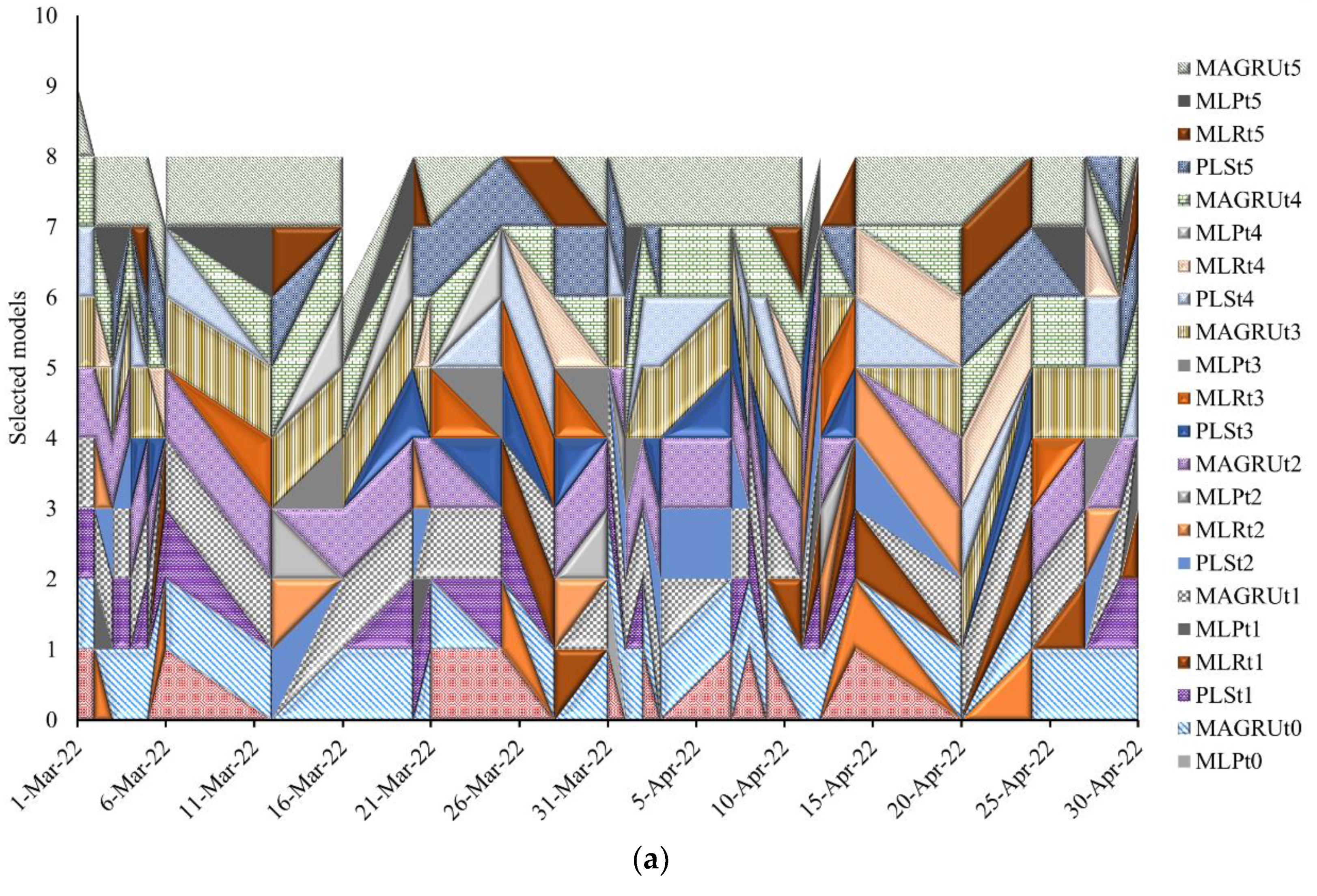
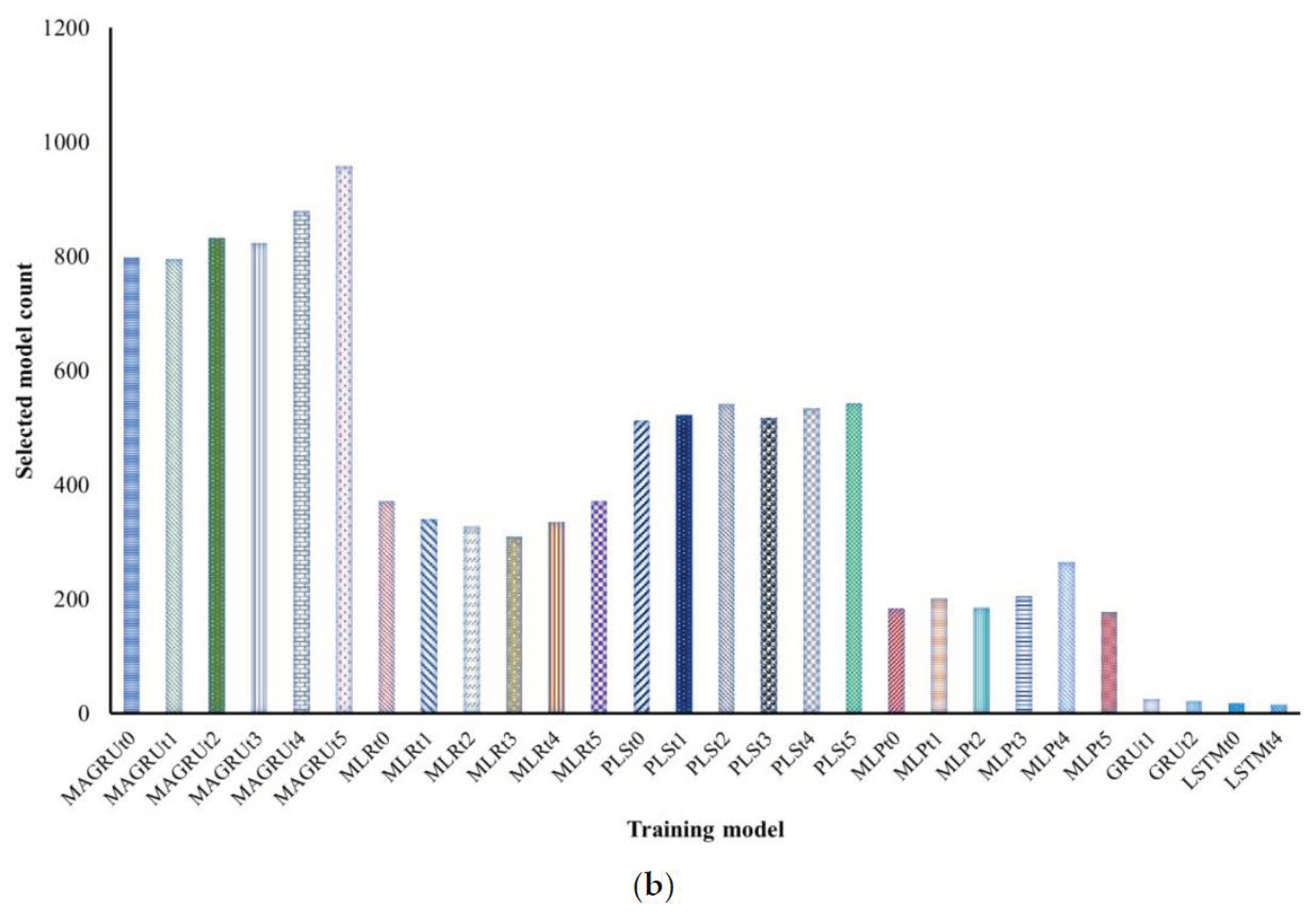
3.2. Determination of the Appropriate Predictive Model Based on Historical Data

This section proposes and compares different algorithms, including PLS, MLR, MLP, LSTM, GRU, and MAGRU. This section’s primary purpose is to determine which approach provides the most accurate predictions with little error. In this respect, MSE was used as the loss function for the training phase of the algorithms, while MAE, RMSE, and R2 were employed as comparison measures. The dataset was additionally preprocessed to eliminate missing values. It should be emphasized that deleting outliers might enhance training outcomes, but it is crucial to retain them to better comprehend the overall picture of the studies, particularly when there are many outliers. Considering this, the dataset’s outliers were maintained. Depending on the quantity of missing data, users may choose an appropriate solution-producing approach. Furthermore, the ideal window size and window aggregation settings in preparation for the final comparisons were used.
Regarding time series data sets, the characteristics of wastewater are reliant on previous time steps. Consequently, “Rolling Forecasting Origin” was used to evaluate forecasting algorithms [39]. In this method, just the subsequent value of effluent TN is prioritized. At each time step, a new observation was added to the training set, which was the precise output from the previous time step. A new model is trained using the updated training set to predict the value of effluent TN. In addition, the performance of the algorithms is only provided on the test data since it offers an objective test against unobserved data to validate the trained model’s consistency. In addition, a batch normalization layer was arbitrarily added between the first and second hidden layers, and linear activation was used to decode the output layer. Moreover, RNN encodes the input based on the number of motor neurons (1 neuron). The output layer is next a dense layer that decodes the instantiated RNN and adapts the output to the dimensions of the desired predicted sequences. The structures of GRU, LSTM, and MAGRU were determined after optimization of the structure. The description of the structures of each technique is detailed in Table 2.
The modeling performance metrics quantify the error that each modeling technique produces. The model with the least values of MAE is the most accurate. The top scores are highlighted in Table 3 for the modeling performance of the water quality variables in the wastewater treatment plant using various modeling techniques. The top eight models are selected based on performance metrics. It shows the randomly picked performance of all methods at different times, where subscripts t0, t1, t2, t3, t4, and t5 show a subset of selected predictive features from RFE.
The modeling performance metrics quantify the error that each modeling technique produces. The MAE for the modeling performance of the water quality variables in the WWTP using various modeling techniques is summarized in Table 3. The top eight models are selected based on performance metrics. It shows the random performance of all methods across the time, where subscripts t0–t5 show a subset of selected features.
The LSTM memory cell incorporation demonstrates the worst performance among the neural models. However, its parameters are adaptable for every time step. The reason for this is that as the input length rises, so does the amount of information stored in each layer of the memory module. During network training, the model will be influenced by these long-term stored correlations while learning the short-term local characteristics of the current input. As a result, the prediction accuracy of the model decreases. The GRU method shows accuracy reported as MAE from 0.62 to 1.88 in the training model, where it shows an acceptable accuracy; however, it suffers from overfitting as for unseen information. According to the RNN methods, the modeling performance is somehow similar; however, comparing the RNN with the MLP, it can be noted that low improvement can be obtained when applying RNN methods in each time step (hourly interval prediction), achieving 11–25% improvement on average. The MLRt2 exhibits the most accurate performance for considering neural models, with an improvement of 8.3% with the MLPt4. The accuracy of the MLR is reported as MAE, where 0.42 was reported as the lowest in the MLRt1, while the highest value of −1.38 was reported in the MLRt0; thus, it is selected as the best model in some training stages.
Furthermore, the multi-attention transformer-based RNN network and statistical method, PLS, resulted in the most accurate model for the prediction of an effluent TN. The performance values of the MAGRU and PLS in the training stage are 0.26 (MAGRt2) and 0.30 (PLSt4), respectively, which outperformed the ML approaches for the modeling task. MAGRU method is selected most of the time as per the performance metrics for the prediction of effluent TN as it shows a low MAE value compared to the other studied methods. The second ranked after MAGRU was the PLS modeling method, which achieved the best results in most cases. The comparison results of the real-time modeling performance based on different ML and AI models are depicted in Figure 9. The layer represents the model selected in time step t.
The MAGRU method reported the most accurate and selective predictive performance among all introduced models in various subsets. Generally, the mean absolute error and higher R2 throughout the data groups, and for modeled parameters of TN, are indications of the MAGRU’s robustness. The PLS obtained the second most accurate model compared to the reported ML models. At the same time, it shows that the MAGRU and PLS models outperform the GRU and LSTM neural networks. The MAE of the PLSt5 approximating wastewater treatment processes was 0.41 for effluent TN, while the MAE of the predicted TN using the MAGRUt5 was 0.28. The rest of the performance for all models can be seen in Figure 9a. Detailed information on the selection of the models can be found in Figures S1–S4 of the Supplementary Information. The total number of counts of each model in the training period can be seen in Figure 9b. It shows that MAGRU was selected most of the time as the best model, where MAGRUt5 is ranked first with a total count of 958.
TN has discharge criteria for WWTPs; hence, it is vital to develop a multi-index prediction model. Based on the study, it has been determined that the prediction accuracy of models constructed using the PLS and MAGRU is high. Consequently, the selected models were used for the prediction of effluent TN. We agree that the following variables are mostly responsible for the significant performance of the multi-attention transformer: (1) The memory module plays a critical role in achieving this outcome by recording local and global correlation dependencies through long-term and short-term memory, respectively. (2) Multisegment prediction reduces the number of repetitive outputs, which effectively reduces the build-up of mistakes. (3) Integrating the time-distributed module into the model makes the model more sensitive to changes in the input data’s scale. This suggests that the difficulty of collecting long- and short-term trends for ultra-long-term prediction grows as the horizon lengthens. All selected models were used in the prediction stage and concatenated to take the average of all eight models for efficient prediction of the multistep ahead effluent TN. The next section explains the prediction performance of the proposed approach.

3.3. Hourly and Multistep Effluent TN Prediction

Any rapid changes in wastewater characteristics in the influent and effluent might result in severe treatment failure, a decrease in the overall remediation effectiveness of WWTPs, and further environmental harm. To assist WWTP management teams to take fast action in response to these concerns, a short-term prediction technique based on hourly regression is a must-have.
To evaluate the effectiveness of the selected algorithms on WWTPs, Figure 10 demonstrates the variation of predicted test data based on the error ratio between predicted and observed data by taking the average of all selected models. The figure depicts standard residual error, and the residual error was small. All selected models performed adequately on the effluent TN dataset, as the errors were not excessively huge, and they were all quite close. Although the errors of each of the eight models were tiny, the number of discrepancies between the point prediction curves and the observed value curves was considerable. The proposed approach was proven to have a positive impact on the effluent TN multistep forward prediction. The MAGRU and PLS model provided the best fitting precision and generalizability for the prediction of effluent TN, as well as reasonably substantial prediction power, allowing for accurate nonlinear modeling in wastewater treatment systems.
To minimize overfitting issues, it is observed that MAGRU and PLS permitted better performance of testing results than training results. In the meantime, Figure 10b demonstrates that the predictions of selected models can capture the variability of effluent TN with the overall efficiency of 98.1% for 1 h future prediction. Results clearly indicate the improved accuracy of the proposed framework in an operational wastewater treatment plant. The suggested method also proved the robustness of predicting the effluent under substantial changes, which would be useful for boosting the alertness of the WWTP operation or altering the urban sewage network in advance to equalize the pollution loading of the influent. As indicated in Figure 10c, the TN content predicted by the suggested method for effluent over-limit discharges was more likely to correspond to reality. The residuals yielded by the proposed approach, in which the values were maintained in the interval of [−4, 4], except for a single point that surpassed these intervals. A quantile–quantile plot of the residuals, as shown in Figure 10d, suggests that these errors have a close to normal distribution and do not show extreme observations, making this a robust method for water quality modeling.
Figure 11 shows the effluent TN predictions for 3 h ahead, which are similar to the findings shown in Figure 10. It is shown in Figure 11a that the suggested modeling framework was able to capture the peak values that were important for operational decision-making. As shown in Figure 11b, an appropriate approximation of the dataset can be shown by looking at the correlation between the present and expected TNeff values during the prediction stage. According to the suggested technique, Figure 11c,d shows the residuals generated by this method, which were kept within the range of [4, 4] except for three points. There are no extreme data in the residuals, and this technique is thus resilient for water quality modeling, as shown by a quantile–quantile plot. Thus, the proposed method can assist in establishing the WWTP’s proactive measures to address potentially aberrant cases.
Since ML algorithms require an understanding of arithmetic and programming languages, a web app was designed to make them more user friendly. The ones of interest must enter wastewater parameters, such as effluent TN, and then the predicted results are readily available. The web application is comprised of four parts: (1) User interface, which is the front-end that accepts user input values and object controls, as well as the program’s layout and appearance; (2) Server function, which is the back-end that processes these input values to finally produce the output results that are finally presented on the website; (3) Database, the cloud that reads and writes real-time sensor data from wastewater treatment plants and saves predicted values; and (4) Algorithms, the application itself that combines.
In terms of model structure and parameter formulation, this work’s outcomes may potentially serve as a preliminary reference for future research. In addition, it is important to note that effluent TN was deliberately chosen as an output variable due to its vital concern over nutrient enrichment, but the web app can also be customized for other wastewater quality parameters (such as TP, NH3, COD, and TSS as output variables), depending on the specific purpose and relevant matter. Overall, this web program provides a comprehensive, easy, and simple method for predicting wastewater quality, hence assisting enterprises with proactive water management techniques. Additionally, this web service can continuously monitor the wastewater quality and warrant the accuracy of the developed framework using ML algorithms. The developed ML framework is applicable to other places, as the work is implemented in various wastewater treatment facilities.

4. Conclusions

For the proper operation and management of WWTPs, early identification of variable influent and effluent concentrations is critical. According to this study’s findings, ML algorithms may be used to predict the quality of wastewater in full-scale WWTPs. Effluent TN concentration is a limiting factor in the formation of eutrophication because its concentration regularly exceeds the standard discharge threshold. In this work, six different ML algorithms ranging from shallow to deep learning architectures were developed to detect effluent TN concentration. As illustrated by the lowest error value, MAGRU, a multi-attention RNN, consistently documented the greatest performance for regression estimation. When it came to computing efficiency, PLS performed well, indicating that this technique was a good fit for effluent TN modeling. Other ML algorithms, on the other hand, fell short due to structural complexity concerns. LSTM did not help to enhance prediction capability; on the contrary, it made the model structure more unstable and noisier. Shallow architectures, such as MLR and MLP, on the other hand, were unable to deal with big datasets that exhibited nonlinear and nonstationary characteristics.
The proposed model was validated with measured effluent data from a full-scale WWTP in South Korea. Effluent TN was best predicted by the suggested prediction model because of the structure’s ability to cope with hourly and peak load from deconstructed sublayers of original data. Due to the high peaks and short- and long-term periodic properties of wastewater discharge, this is a critical benefit for the suggested framework Incoming influent, a major contributor to effluent variability, and load factors relevant to actual WWTP operations were included in the prediction model, and it performed well. Modern urban activities are becoming more automated and computerized, making intelligent administration of wastewater treatment systems possible. A new and effective effort is made in the data preprocessing technique to use time-frequency transformation algorithms to make outliers and nonaligned data play beneficial roles. This study’s high-frequency indicators have a time window of between one and three hours.

Supplementary Materials

The following supporting information can be downloaded at: https://www.mdpi.com/article/10.3390/w14193147/s1, Figures S1–S4: Results of the selection of different training models in time series.

Author Contributions

Conceptualization, U.S., J.K., and G.R.; methodology, U.S., J.K., and G.R.; software, U.S., J.K., G.P., and G.R.; validation, U.S.; formal analysis, U.S.; investigation, U.S., J.K., and G.P.; data curation, U.S., J.K., and G.R.; writing—original draft preparation, U.S.; writing—review and editing, U.S.; visualization, U.S., J.K., and G.R.; supervision, J.K. and G.P.; project administration, K.Y.; funding acquisition, K.Y. All authors have read and agreed to the published version of the manuscript.

Funding

This research was supported by the Korea Environment Industry & Technology Institute (KEITI) through the “Prospective Green Technology Innovation Project” (No. 2021003160003 and No. 2021003170009), funded by the Korea Ministry of Environment (MOE), and support was provided by the MOE as “Global Top Project” (No. 2019002210001).

Data Availability Statement

The raw data supporting the conclusions of this study will be made available from the corresponding author upon request.

Conflicts of Interest

The authors declare no conflict of interest.

References

  1. Safder, U.; Loy-Benitez, J.; Nguyen, H.-T.; Yoo, C. A Hybrid Extreme Learning Machine and Deep Belief Network Framework for Sludge Bulking Monitoring in a Dynamic Wastewater Treatment Process. J. Water Process Eng. 2022, 46, 102580. [Google Scholar] [CrossRef]
  2. Safder, U.; Tariq, S.; Yoo, C. Multilevel Optimization Framework to Support Self-Sustainability of Industrial Processes for Energy/Material Recovery Using Circular Integration Concept. Appl. Energy 2022, 324, 119685. [Google Scholar] [CrossRef]
  3. Safder, U.; Rana, M.A.; Yoo, C. Feasibility Study and Performance Assessment of a New Tri-Generation Integrated System for Power, Cooling, and Freshwater Production. Desalin. WATER Treat. 2020, 183, 63–72. [Google Scholar] [CrossRef]
  4. Vilela, P.; Safder, U.; Heo, S.; Nguyen, H.; Lim, J.Y.; Nam, K.; Oh, T.; Yoo, C. Dynamic Calibration of Process-Wide Partial-Nitritation Modeling with Airlift Granular for Nitrogen Removal in a Full-Scale Wastewater Treatment Plant. Chemosphere 2022, 305, 135411. [Google Scholar] [CrossRef] [PubMed]
  5. Salgot, M.; Folch, M. Wastewater Treatment and Water Reuse. Curr. Opin. Environ. Sci. Heal. 2018, 2, 64–74. [Google Scholar] [CrossRef]
  6. Karunanidhi, D.; Aravinthasamy, P.; Subramani, T.; Roy, P.D.; Srinivasamoorthy, K. Risk of Fluoride-Rich Groundwater on Human Health: Remediation Through Managed Aquifer Recharge in a Hard Rock Terrain, South India. Nat. Resour. Res. 2020, 29, 2369–2395. [Google Scholar] [CrossRef]
  7. Jaramillo, F.; Orchard, M.; Muñoz, C.; Zamorano, M.; Antileo, C. Advanced Strategies to Improve Nitrification Process in Sequencing Batch Reactors—A Review. J. Environ. Manage. 2018, 218, 154–164. [Google Scholar] [CrossRef]
  8. Safder, U.; Nam, K.; Kim, D.; Shahlaei, M.; Yoo, C. Quantitative Structure-Property Relationship (QSPR) Models for Predicting the Physicochemical Properties of Polychlorinated Biphenyls (PCBs) Using Deep Belief Network. Ecotoxicol. Environ. Saf. 2018, 162, 61. [Google Scholar] [CrossRef]
  9. Fan, M.; Hu, J.; Cao, R.; Ruan, W.; Wei, X. A Review on Experimental Design for Pollutants Removal in Water Treatment with the Aid of Artificial Intelligence. Chemosphere 2018, 200, 330–343. [Google Scholar] [CrossRef]
  10. Elkiran, G.; Nourani, V.; Abba, S.I. Multi-Step Ahead Modelling of River Water Quality Parameters Using Ensemble Artificial Intelligence-Based Approach. J. Hydrol. 2019, 577, 123962. [Google Scholar] [CrossRef]
  11. Zhao, L.; Dai, T.; Qiao, Z.; Sun, P.; Hao, J.; Yang, Y. Application of Artificial Intelligence to Wastewater Treatment: A Bibliometric Analysis and Systematic Review of Technology, Economy, Management, and Wastewater Reuse. Process Saf. Environ. Prot. 2020, 133, 169–182. [Google Scholar] [CrossRef]
  12. Bagheri, M.; Bazvand, A.; Ehteshami, M. Application of Artificial Intelligence for the Management of Landfill Leachate Penetration into Groundwater, and Assessment of Its Environmental Impacts. J. Clean. Prod. 2017, 149, 784–796. [Google Scholar] [CrossRef]
  13. Mohammad, A.T.; Al-Obaidi, M.A.; Hameed, E.M.; Basheer, B.N.; Mujtaba, I.M. Modelling the Chlorophenol Removal from Wastewater via Reverse Osmosis Process Using a Multilayer Artificial Neural Network with Genetic Algorithm. J. Water Process Eng. 2020, 33, 100993. [Google Scholar] [CrossRef]
  14. Poznyak, A.; Chairez, I.; Poznyak, T. A Survey on Artificial Neural Networks Application for Identification and Control in Environmental Engineering: Biological and Chemical Systems with Uncertain Models. Annu. Rev. Control 2019, 48, 250–272. [Google Scholar] [CrossRef]
  15. Mokhtari, H.A.; Bagheri, M.; Mirbagheri, S.A.; Akbari, A. Performance Evaluation and Modelling of an Integrated Municipal Wastewater Treatment System Using Neural Networks. Water Environ. J. 2020, 34, 622–634. [Google Scholar] [CrossRef]
  16. Deng, Y.; Zhou, X.; Shen, J.; Xiao, G.; Hong, H.; Lin, H.; Wu, F.; Liao, B.-Q. New Methods Based on Back Propagation (BP) and Radial Basis Function (RBF) Artificial Neural Networks (ANNs) for Predicting the Occurrence of Haloketones in Tap Water. Sci. Total Environ. 2021, 772, 145534. [Google Scholar] [CrossRef]
  17. Noori, N.; Kalin, L.; Isik, S. Water Quality Prediction Using SWAT-ANN Coupled Approach. J. Hydrol. 2020, 590, 125220. [Google Scholar] [CrossRef]
  18. Bagheri, M.; Akbari, A.; Mirbagheri, S.A. Advanced Control of Membrane Fouling in Filtration Systems Using Artificial Intelligence and Machine Learning Techniques: A Critical Review. Process Saf. Environ. Prot. 2019, 123, 229–252. [Google Scholar] [CrossRef]
  19. Ma, J.; Ding, Y.; Cheng, J.C.P.; Jiang, F.; Xu, Z. Soft Detection of 5-Day BOD with Sparse Matrix in City Harbor Water Using Deep Learning Techniques. Water Res. 2020, 170, 115350. [Google Scholar] [CrossRef]
  20. Zhang, Y.-F.; Fitch, P.; Thorburn, P.J. Predicting the Trend of Dissolved Oxygen Based on the KPCA-RNN Model. Water 2020, 12, 585. [Google Scholar] [CrossRef]
  21. Jiang, Y.; Li, C.; Sun, L.; Guo, D.; Zhang, Y.; Wang, W. A Deep Learning Algorithm for Multi-Source Data Fusion to Predict Water Quality of Urban Sewer Networks. J. Clean. Prod. 2021, 318, 128533. [Google Scholar] [CrossRef]
  22. Farhi, N.; Kohen, E.; Mamane, H.; Shavitt, Y. Prediction of Wastewater Treatment Quality Using LSTM Neural Network. Environ. Technol. Innov. 2021, 23, 101632. [Google Scholar] [CrossRef]
  23. Xu, R.; Deng, X.; Wan, H.; Cai, Y.; Pan, X. A Deep Learning Method to Repair Atmospheric Environmental Quality Data Based on Gaussian Diffusion. J. Clean. Prod. 2021, 308, 127446. [Google Scholar] [CrossRef]
  24. Qin, Y.; Song, D.; Chen, H.; Cheng, W.; Jiang, G.; Cottrell, G. A Dual-Stage Attention-Based Recurrent Neural Network for Time Series Prediction. arXiv preprint 2017, arXiv:1704.02971. [Google Scholar]
  25. Liu, H.; Motoda, H. Feature Selection for Knowledge Discovery and Data Mining; Springer: Boston, MA, USA, 1998; ISBN 978-1-4613-7604-0. [Google Scholar]
  26. Dey, S.K.; Rahman, M.M. Flow Based Anomaly Detection in Software Defined Networking: A Deep Learning Approach with Feature Selection Method. In Proceedings of the 2018 4th International Conference on Electrical Engineering and Information & Communication Technology (iCEEiCT), Bangladesh, 13–15 September 2018; IEEE: Piscataway, NJ, USA, 2018; pp. 630–635. [Google Scholar]
  27. Mishra, B.K.; Regmi, R.K.; Masago, Y.; Fukushi, K.; Kumar, P.; Saraswat, C. Assessment of Bagmati River Pollution in Kathmandu Valley: Scenario-Based Modeling and Analysis for Sustainable Urban Development. Sustain. Water Qual. Ecol. 2017, 9–10, 67–77. [Google Scholar] [CrossRef]
  28. Singh, A.; Jain, A. Adaptive Credit Card Fraud Detection Techniques Based on Feature Selection Method; Springer: Singapore, 2019; pp. 167–178. [Google Scholar]
  29. Aggarwal, C.C.; Reddy, C.K. (Eds.) Data Clustering; Chapman and Hall/CRC: New York, NY, USA, 2016; ISBN 9781315373515. [Google Scholar] [CrossRef]
  30. Nkiama, H.; Zainudeen, S.; Saidu, M. A Subset Feature Elimination Mechanism for Intrusion Detection System. Int. J. Adv. Comput. Sci. Appl. 2016, 7, 419. [Google Scholar] [CrossRef] [Green Version]
  31. Tian, Z.; Gu, B.; Yang, L.; Lu, Y. Hybrid ANN–PLS Approach to Scroll Compressor Thermodynamic Performance Prediction. Appl. Therm. Eng. 2015, 77, 113–120. [Google Scholar] [CrossRef]
  32. Safder, U.; Nam, K.J.; Kim, D.; Heo, S.K.; Yoo, C.K. A Real Time QSAR-Driven Toxicity Evaluation and Monitoring of Iron Containing Fine Particulate Matters in Indoor Subway Stations. Ecotoxicol. Environ. Saf. 2019, 169, 361–369. [Google Scholar] [CrossRef]
  33. Pradhan, B.; Lee, S. Landslide Susceptibility Assessment and Factor Effect Analysis: Backpropagation Artificial Neural Networks and Their Comparison with Frequency Ratio and Bivariate Logistic Regression Modelling. Environ. Model. Softw. 2010, 25, 747–759. [Google Scholar] [CrossRef]
  34. Elmaz, F.; Eyckerman, R.; Casteels, W.; Latré, S.; Hellinckx, P. CNN-LSTM Architecture for Predictive Indoor Temperature Modeling. Build. Environ. 2021, 206, 108327. [Google Scholar] [CrossRef]
  35. Mallick, R.; Yebda, T.; Benois-Pineau, J.; Zemmari, A.; Pech, M.; Amieva, H. A GRU Neural Network with Attention Mechanism for Detection of Risk Situations on Multimodal Lifelog Data. In Proceedings of the 2021 International Conference on Content-Based Multimedia Indexing (CBMI), Lille, France, 28–30 June 2021; IEEE: Piscataway, NJ, USA, 2021; pp. 1–6. [Google Scholar]
  36. Kjell, O.N.E.; Sikström, S.; Kjell, K.; Schwartz, H.A. Natural Language Analyzed with AI-Based Transformers Predict Traditional Subjective Well-Being Measures Approaching the Theoretical Upper Limits in Accuracy. Sci. Rep. 2022, 12, 3918. [Google Scholar] [CrossRef] [PubMed]
  37. Arroyo, D.M.; Postels, J.; Tombari, F. Variational Transformer Networks for Layout Generation. In Proceedings of the IEEE/CVF Conference on Computer Vision and Pattern Recognition (CVPR), Nashville, TN, USA, 19–25 June 2021. [Google Scholar] [CrossRef]
  38. Pei, W.; Baltrušaitis, T.; Tax, D.M.J.; Morency, L.-P. Temporal Attention-Gated Model for Robust Sequence Classification. In Proceedings of the IEEE Conference on Computer Vision and Pattern Recognition, Las Vegas, NV, USA, 26 June – 1 July 2016. [Google Scholar]
  39. Hyndman, R.J.; Ahmed, R.A.; Athanasopoulos, G.; Shang, H.L. Optimal Combination Forecasts for Hierarchical Time Series. Comput. Stat. Data Anal. 2011, 55, 2579–2589. [Google Scholar] [CrossRef]
Figure 1. Conceptual configuration of the wastewater treatment plant.
Water 14 03147 g001
Figure 2. Influent conditions from the full-scale WWTP study.
Water 14 03147 g002
Figure 3. Architecture representation of the sensor and wastewater process feature selection.
Water 14 03147 g003
Figure 4. Architecture of MLP modeling for predicting future WWTP effluent water quality.
Water 14 03147 g004
Figure 5. Structure diagram of the LSTM network for multiple-step ahead TN prediction.
Water 14 03147 g005
Figure 6. Schematic representation of Transformer with multihead attention.
Water 14 03147 g006
Figure 7. Conceptual configuration of proposed multistep effluent TN prediction at full-scale WWTP.
Water 14 03147 g007
Figure 8. Selection of features using RFE in time series.
Water 14 03147 g008
Figure 9. Results of the (a) selection of different training models in time series (b) number of counts of selected models in training period.
Water 14 03147 g009aWater 14 03147 g009b
Figure 10. One-hour ahead prediction performance visualization of (a) a time series of predicted effluent TN, (b) a scatter plot of predicted and current TN values, (c) the generated residuals, and (d) the quantile–quantile plot for model residuals.
Water 14 03147 g010
Figure 11. Three-hour ahead prediction performance visualization of (a) a time series of predicted effluent TN, (b) a scatter plot of predicted and current TN values, (c) the generated residuals, and (d) the quantile–quantile plot for model residuals.
Water 14 03147 g011
Table 1. Process variables in an H-municipal full-scale treatment plant.
Influent ParameterDescriptionUnitMeanStandard Deviation
QinInfluent flowratem3/day83.0516.84
CODinChemical oxygen demandmg/L13.062.43
MLSSMixed liquor suspended solidsmg/L2892.07335.43
TSSinTotal suspended solidsmg/L2.760.74
TNinTotal nitrogenmg/L8.132.27
TPinTotal phosphorousmg/L0.350.16
Table 2. Description of the structures of the different DL models for TN prediction.
GRULSTMMAGRU
General training componentsBatch size: 2048
Epochs: 500
Validation split: 0.2
Early stopping patience: 10
Loss function: mean squared error
Optimizer: Adam
Batch size: 128
Epochs: 100
Model checkpoint
Optimizer: Adam
Learning rate: 0.001
Batch size: 3
Epochs: 100
Validation split: 0.2
Loss function: mean squared error
Optimizer: Adam
Hyperparameters descriptionHidden layer 1: 256 memory cells
Hidden layer 2: 128 memory cells
Dropout: 0.15
Learning rate: dynamic
Hidden layer 1: 32 neurons (ReLU)
Hidden layer 2: 16 neurons (ReLU)
Dropout: 0.15
Learning rate: dynamic
Encoder 1: 64 neurons (ReLU)
Encoder 2: 64 neurons (ReLU)
Hidden layer 1: 16
Time distributed 1: 64
Time distributed 2: 32
Max Pooling: 64
Table 3. Performance comparison of different models.
Models/Time1 March 2022 02:00 h2 March 2022 04:00 h10 March 2022 13:00 h15 March 2022 22:00 h28 March 2022 06:00 h5 April 2022 11:00 h15 April 2022 09:00 h26 April 2022 15:00 h
Score-MAE
PLSt00.5610.8080.8610.5720.7150.4270.4320.503
MLRt00.5770.7080.7160.5640.6310.4350.4410.432
MLPt00.7720.9790.7880.6450.8811.3860.7060.437
GRUt00.9731.0130.8931.0541.0681.4751.8250.969
LSTMt00.6880.8760.8450.7650.7880.6790.9870.906
MAGRUt00.4360.3980.5500.4250.9610.3740.5880.416
PLSt10.4000.5530.8780.5930.5951.3570.4460.672
MLRt10.4780.5450.7300.5620.4820.9280.4280.554
MLPt10.5300.7560.6400.4920.5751.6480.6560.541
GRUt10.6261.0150.8850.6761.0801.4841.8531.375
LSTMt10.7030.7540.8450.7880.7210.9861.0100.906
MAGRUt10.3040.4230.5510.3210.3590.3690.6690.411
PLSt20.4590.6111.7881.7630.5390.3120.4840.369
MLRt20.5130.5500.9321.0530.4730.4340.4270.434
MLPt20.6530.5740.6370.9550.5994.6010.7160.426
GRUt20.9411.0040.9351.0571.0611.4761.8870.876
LSTMt20.6890.7570.9860.8100.7210.7540.9870.906
MAGRUt20.3950.5930.4060.2640.6310.3300.5840.481
PLSt30.4250.4010.8460.5890.5700.4170.5180.356
MLRt30.4790.4890.6950.5680.4680.4700.4260.431
MLPt30.4950.7330.6550.6080.6601.7370.5490.457
GRUt30.9401.0370.8891.1831.0751.4771.8560.877
LSTMt30.6890.7520.8410.7650.7210.6790.9870.906
MAGRUt30.4040.3980.4530.5570.3500.3300.6280.313
PLSt40.4050.4280.8440.5250.5440.3030.8430.407
MLRt40.4790.4860.7000.5560.4840.4390.6010.444
MLPt40.5230.5190.8510.5880.6051.9540.9680.417
GRUt40.9421.0060.8951.0741.0821.4771.8840.924
LSTMt40.7160.7540.8450.7650.7210.6801.0530.906
MAGRUt40.4080.3890.3710.4920.3670.3900.6110.307
PLSt50.5140.4091.0060.5420.5510.8300.9263.337
MLRt50.5710.4890.8060.5630.5250.5800.6091.384
MLPt50.7640.6730.8190.5991.1191.2490.6831.421
GRUt50.9461.0260.8931.0501.0660.4990.8811.461
LSTMt50.7330.7540.9030.7650.7210.6790.9871.132
MAGRUt50.3760.4060.4470.4270.4940.2860.4380.305
Publisher’s Note: MDPI stays neutral with regard to jurisdictional claims in published maps and institutional affiliations.

