
Extreme Precipitation Events on the East Coast of Brazil’s Northeast: Numerical and Diagnostic Analysis


1
National Institute for Space Research, Cachoeira Paulista 12630-000, Brazil
2
National Center for Monitoring and Early Warning of Natural Disasters, São José dos Campos 12247-016, Brazil
*
Author to whom correspondence should be addressed.
Water 2022, 14(19), 3135; https://doi.org/10.3390/w14193135
Submission received: 17 August 2022
/
Revised: 25 September 2022
/
Accepted: 30 September 2022
/
Published: 4 October 2022
(This article belongs to the Section Hydrology)
Abstract
:The Northeast of Brazil (NEB) is the region with the highest number of municipal decrees of emergency situation declaration caused by weather events in the period from 2013 to 2022 and with the highest rate of natural disasters per risk area. In the NEB, the city of Recife and its metropolitan region are the biggest localities with populations in risk areas. Focusing on this region, five events of extreme precipitation were chosen for simulations using the WRF model and diagnostics analyses. First, a set of configurations of the model was tested, including 11 microphysics (MPH) schemes, 9 planetary boundary layer (PBL) schemes, 5 cumulus (CUM), and 7 surface layer (SFC) schemes. Then, through diagnostic analysis, the conditional instability, the moisture supply at low levels, and the support of the medium and high levels in storm formation were verified. The model’s configurations were verified by 298 rain gauges with hourly registrations through statistical metrics such as bias, MSE, standard deviation, and Pearson’s correlation, and demonstrated that the MPH schemes of Thompson Aerosol-Aware and NSSL + CCM, ACM2, MYJ for the PBL, KFCuP for CUM, and RUC for SFC were considered the best. All the cases were better with CUM parametrizations turned on. In all cases, diagnostics analyses highlighted the strong moisture flux convergence at the low levels, the presence of wind shear on the middle layer, weak cyclonic vorticity advection at high levels, and CAPE values around 1500 J/kg, in addition to an inverse relationship between wind shear action and CAPE values. This work is part of the national strategy for monitoring, diagnosis, and modeling of information that can minimize or even prevent damage caused by severe precipitation events.
1. Introduction
The history of socioeconomic development of Brazil is characterized by different uses of land and different patterns of land occupation, revealing a heterogeneous population distribution. This disorderly occupation when exposed to natural climate variability and the natural susceptibility of the regions leads to landslides and floods [1], which are disasters that cause the maximum number of deaths in Brazil [2]. Numerous studies have investigated the occurrence of floods, flash floods, and landslides triggered by severe weather events delivering large amounts of rainfall [3,4,5,6,7,8]. Extreme hydrometeorological events, responsible for large amounts of precipitation, have become more frequent and intense in recent decades [9]. Extreme events are also components of natural climate variability, and their periodicity and intensity, whether natural or induced by human activities, may change [10]. Such phenomena can impact society, causing natural disasters, depending on site vulnerabilities.
To respond to the growing number of natural disasters, the Brazilian government has implemented the National Plan for Risk Management and Disaster Response [11]. Following a dialogue among the three spheres of public administration (federal, state, and municipal), four axes of governmental action were elaborated for the prevention of natural disasters: (i) mapping, focused on producing susceptibility maps, risk sectorization maps, and geotechnical maps, (ii) monitoring and early warning, which involves issuing alerts based on risk analysis of potentially adverse conditions using modeling studies and systematic monitoring of data from observation networks distributed throughout the country, (iii) prevention, which involves the planning and execution of preventive intervention works to avoid risk situations and take corrective measures, and (iv) disaster response, involving actions directed toward providing relief and assistance to and reconstructing areas affected by natural disasters. This work, through modeling studies for a better representation of extreme rainfall events, falls under thematic axis (v).
From a physical point of view, Brazil is more easily affected by disasters of this nature due to its location in the tropical region [12], where the primary source of energy is latent heat release, which occurs in association with convective cloud systems, although much of the precipitation also comes from stratiform cloud regions within mesoscale systems. In tropical regions, there is a strong interaction between cumulus convection and mesoscale and large-scale circulations. Furthermore, the distribution of diabatic heating in the tropics is influenced by variations in sea surface temperature, which is strongly influenced by atmospheric movements. Therefore, to understand tropical circulations, one must consider equatorial wave dynamics, the interactions among cumulus convection, mesoscale circulations, larger-scale motions, and ocean–atmosphere interactions [13].
In Brazil, especially in the NEB, precipitation presents intense spatiotemporal variability, with strong rainy episodes interspersed with long drought periods [14,15]. Atmospheric modeling is one of the main tools for forecasting severe rainfall events [16], despite the several associated challenges, such as the already mentioned strong spatiotemporal variability of precipitation, highly isolated events triggered by local-scale factors, and a lack of full understanding of related physical processes, in addition to the difficulty in verifying the model results, which may require a dense observation network [17]. Gebrechorkos et al. [18] evaluated the performance of five models for average and extreme precipitation events and concluded that all models perform well for medium values in the short- and long-term forecast but the forecast ability is poor for days with heavy precipitation. Several studies using the Weather Research and Forecasting (WRF) model [19] have shown that the model is able to represent extreme precipitation events on both daily and sub-daily scales [20,21,22,23].
The equations of numerical weather prediction (NWP) models are solved at different grid points on the model as a finite element unit, usually on a regular grid. However, many processes are difficult to describe completely, especially if they occur at scales smaller than the resolution of the model. For that, parameterization processes are used that try to represent by approximation, as well as it is possible to, the behavior of particles based on physical laws and empirical observations [24]. In that way, models depend on various physical packages, some of which use approximations for processes that are relatively small compared to the model grid. Thus, atmospheric characteristics can vary greatly, and the optimal combination of these physical packages varies by region [25]. In atmospheric modeling, precipitation processes are fundamentally associated with (i) microphysics parameterizations, which govern the formation, growth, and dissipation of cloud particles [26], (ii) cumulus parameterizations, which represent a series of functions, for example, vertical distribution of heating/cooling and drying/humidification, convection mass transport, generation of the liquid and ice phases of water, interactions with the planetary boundary layer (PBL), interactions with radiation, and mechanical interactions with the mean flow [27], (iii) PBL parameterizations, which can modulate the representation of turbulent mixing in the lower troposphere through the kinematic and thermodynamic vertical profiles that directly influence the buoyancy representation and vertical wind shear, in addition to the evolution of precipitation [28,29], and (iv) land surface parameterization, which controls heat and moisture fluxes of the soil and provides the model with the inputs of heat, moisture, and ground radiation that affect the input variables for other parameterizations and which, despite being less investigated in NWP sensitivity studies, plays an important role in the diurnal precipitation cycle [25,30].
Several studies have investigated the contribution of microphysics and cumulus schemes in severe rainfall events [31,32,33,34], with some results indicating that (i) the additional computational cost of using more sophisticated schemes does not always ensure a better forecast, (ii) there is a larger contribution from microphysics than from cumulus schemes for high-resolution simulations, (iii) rainfall depends on the mixing ratio of rainwater concentrated between low and medium levels, and (iv) different uses of physical parameterizations can cause a larger scatter in the ensemble prediction than the scatter caused by initially perturbed conditions. In NWP, a range of model resolutions over which it is not clear whether the process should be parameterized and where parameterization schemes are designed to represent sub-grid-scale processes that are not explicitly resolved because they are spatially or temporally too small scale, too complex and expensive, or not well understood is called “gray zone” [33]. Jeworrek et al. [33], in a comprehensive review of cumulus and microphysics parameterizations across the convective gray zone, obtained better results for high-resolution simulations with the cumulus parameterization on, but caution that small-scale detailing and noise can contribute to decreased forecasting ability and therefore each model configuration should have its own evaluation. Further studies have shown that activating the cumulus parameterization to high resolution can improve precipitation forecasting [35,36], whereas others have shown significant improvement in explicitly calculated convection in complex terrain regions and less significant improvement in flat regions [37].
Some studies have verified the influence of PBL schemes [28,38,39], indicating that schemes with a non-local resolution, which consider the deep layer covering the multiple levels and represent the effects of vertical mixing by the PBL, are more susceptible to unstable stratifications producing stronger turbulent mixing than schemes with a local resolution, which only consider the immediately adjacent levels in the model, are applicable to stable stratifications, and produce less turbulent mixing. As for the sensitivity studies of the surface models that control the processes of moisture, heat, and momentum exchange between the surface and the atmosphere and also control the meteorological fields near the surface, they are sensitive to PBL processes. Studies such as those by He et al. [40] and López-Bravo et al. [41] suggest that the uncertainties of the surface models, for example, changes in the extent of urban areas and changes associated with dynamic and thermodynamic variables, have induced local circulations and influenced temperature, precipitation, and wind fields.
Stensrud et al. [42] predicted that by the middle of the year 2020, due to the usefulness of high-resolution forecasts and the rapid and continuous increase in computing power, NWP would become an important component of the convective-scale warning system. The high resolution of the models could provide information about the evolution and structure of the storms, and the models must be initiated with an accurate representation of the convection, so as to obtain the necessary correspondence between what was forecast and what is observed. The challenges in achieving this goal included improvements in data assimilation methods, increased use of radar observations, and improvements in the parameterization schemes of the models, in addition to a complete understanding of the forces that initiate and organize severe storms, as well as the environmental parameters that allow the forces to be identified and monitored [43].
Severe storm events develop quickly and have significant consequences for society and the economy, which is why it is essential to quickly recognize the development of conditions that lead to the formation of such events. This is done efficiently through studies that determine the atmospheric environment prior to and during a storm. Taszarek et al. [44] stated that in the long term, the environment characteristics of severe storms (conditional instability, availability of moisture at low levels, wind initiation, and shear mechanism) only partially follow the expectations of the warming climate, that is, despite the increased instability, the environment may be less favorable for thunderstorms due to stronger inhibition energy and lower moisture availability. To explore the relationship between atmospheric parameters and the occurrence of convective thunderstorms, Westermayer et al. [45] used six years of reanalysis data. They found that (i) instability is important up to a certain amount, (ii) approximate convective available potential energy (CAPE) values between 200 and 400 J·kg−1 are more important for the occurrence of lightning strikes than larger values, (iii) the availability of moisture in the lower troposphere has a greater influence on the occurrence of thunderstorms, and (iv) wind shear plays an important role, but only when it occurs at low or high values, with a lower probability of occurrence for intermediate values.
Environments with various combinations of CAPE and wind shear, which can occur at all times and in all seasons, are capable of producing severe weather. Sherburn and Parker [46] presented a climatology for severe weather environments, starting from high shear values and low CAPE values, and introduced new parameters, such as the lapse rate at low and medium levels and wind and shear at multiple levels, as statistically more skillful indicators for forecasting severe weather. Poletti et al. [47] also presented a study based on meteorological indices to predict severe storms. They used a checklist-based tool that took into account physical and thermodynamic processes directed at storm formation, evolution, and organization. One of the main conclusions was the recognition of the seasonal dependence of some indices, suggesting the formulation of two new versions of the identification tool, one for the warm season and one for the cold season. Fabry [48] summarized the main ingredients necessary for a severe storm to occur: (i) a high CAPE value, (ii) some initial resistance to convection, or convective inhibition (CINE), (iii) a continuous supply of moisture; (iv) some support from the high levels, (v) wind shear, especially at low and medium levels, and (vi) convergence at low levels to break locally the CINE resistance. Instability determines the potential for vertical air acceleration, whereas wind shear shapes the storm and influences its evolution. Finally, a lifting mechanism, such as a cold front, sea breeze, or smaller-scale convergence patterns, also determines the location, shape, and extent of the convection.
Due to a scarcity of studies on modeling of severe rainfall events and storm formation dynamics on the east coast of the NEB, this study aims to identify the WRF model settings that have the greatest success in predicting severe rainfall events in the NEB, as well as to analyze the behavior of the meteorological variables associated with the actuation of these storms.
2. Materials and Methods
2.1. Study Area
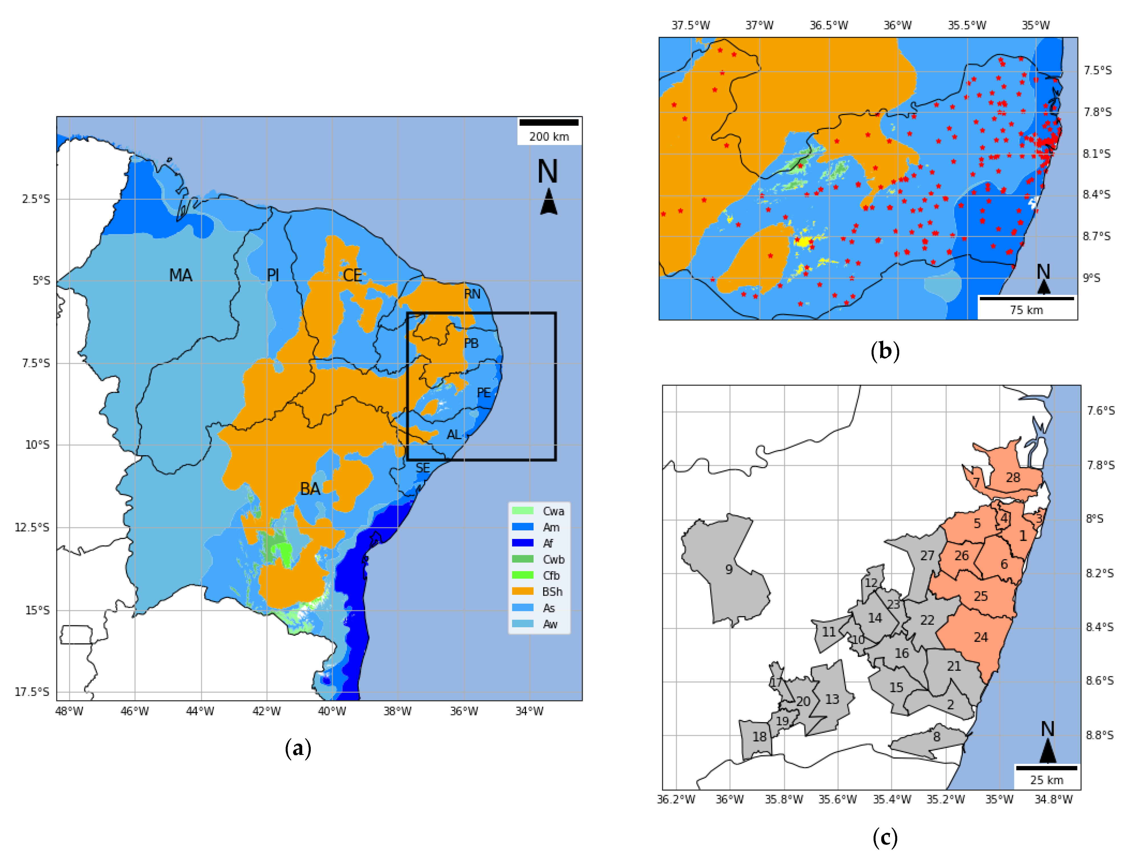
The NEB represents 21.25% of Brazilian territory, with three predominant climate types [49]: (i) humid coastal, from the coast of the state of Bahia to the coast of the state of Rio Grande do Norte, (ii) tropical, in parts of the states of Bahia, Ceará, Maranhão, and Piauí, and (iii) tropical semi-arid, in the countryside of all the states of the region except Maranhão (Figure 1a). The region presents high temperatures, with an annual average between 20 °C and 28 °C, and a small thermal amplitude. The rainfall is irregular, with annual values higher than 2000 mm in the coastal region and less than 500 mm in the inland areas [50]. The NEB had the highest number of abnormalities, as declared by municipal ordinances, in the period from 1 January 2013 to 5 April 2022, and was also the region with the highest rate of events per risk area [51,52]. The metropolitan region of the city of Recife (municipalities with a red background in Figure 1c) has the largest coverage of population in risk areas and the second-highest number of people in risk areas [53].
2.2. Data Set
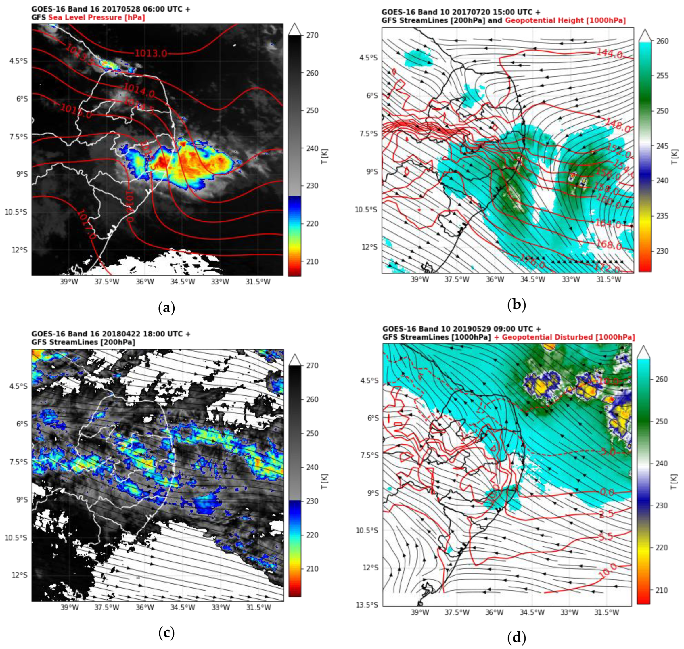
The National Center for Monitoring and Early Warning of Natural Disasters (CEMADEN in Portuguese abbreviation) maintains a platform (Brazilian Early Warning System (BEWS)) for registering the occurrence of natural disasters in Brazil [54]. Via this platform, details about geohydrological disaster events, such as locality, date and time of the opening and closing of the alerts, the description of the event, alert levels, accuracy of time and location, magnitude or scope of the alerts, human damage, and the sources of the information records, are registered. Using this database, five severe rainfall events were chosen between the years 2017 and 2019; these were confirmed to be natural disasters by government authorities in the eastern Pernambuco state (Figure 2a–e). For each of these events, sensitivity tests were performed through simulations with the WRF model (described in Section 2.3). Diagnostic analyses (described in Section 2.5) of intense precipitation episodes were also performed in the intersection regions between the largest precipitation events and where disaster alerts were in effect (yellow boxes in Figure 2).
CEMADEN’s automatic rain gauge network was used (http://www2.cemaden.gov.br/mapainterativo/ (accessed on 5 May 2021)) to analyze the rainfall intensity in the state of Pernambuco. In this state, the total quantity varied according to the date of the analyzed event due to the constant equipment maintenance, but it has a maximum number of 298 rain gauges and a minimum of 170, represented by the red stars in Figure 1b.
To classify the synoptic and mesoscale systems, as well as the initial and boundary conditions, in the numerical simulations, we used the analyses in the synoptic timetables and the 3-h forecasts of the Global Forecast System (GFS) of the National Centers for Environmental Prediction (NCEP) with grid spacing of 0.25° latitude and longitude (https://rda.ucar.edu/datasets/ds084.1/ (accessed on 23 February 2021)) and GOES16 satellite data (https://noaa-goes16.s3.amazonaws.com/index.html#ABI-L2-CMIPF/ (accessed on 15 May 2021)). To classify the systems, the surface pressure fields, streamlines and wind magnitude at various levels, geopotential height, wind divergence, and near-surface moisture flux convergence (MFC) were analyzed.
2.3. Numerical Simulations
Table 1 presents the five severe rainfall events that were selected for sensitivity testing with the WRF model (version 4.2) according to the use of the microphysics, the planetary boundary layer, cumulus, and land surface parameterizations. Table 2 displays the set of tested schemes and their references. These schemes were chosen because the official model documentation states that they can be used in high resolution. For each event analyzed, 24 h of simulation was performed with initialization, if possible, at least 6 h before the onset of precipitation.
The region used in the numerical simulations is demarcated by the black rectangle in Figure 1a. The simulations were performed in two nested regions following a one-way nesting strategy, the parent domain, with a 5.0 km resolution and a 200 × 200-point grid, and the internal domain (used in this study), with 2.5 km resolution and a 201 × 201-point grid, both centered at 8.19203° S latitude and 35.46051° W longitude, with the model top at 50 hPa and 40 levels using the terrain-following vertical coordinate. For the initial and boundary conditions, the GFS analysis and forecasts every 3 h were used. The time step of the WRF model was set to 15 s, and the output frequency of the WRF model was 1 h.
All the possible combinations between the tested physical schemes would be on the order of thousands of simulations. To reduce the high computational cost of the simulations, we evaluated the physical schemes within their own physical type, choosing the most skillful scheme among them and then analyzing the next set of physical options [55]. After the simulations concerning the microphysics parameterization schemes, it is possible to verify the PBL schemes because there is no direct interaction with microphysics, followed by the cumulus parameterizations, which do not interact with the PBL, and finally land surface schemes [56]. Each experiment set started with the RRTMG shortwave and longwave radiation schemes (invariant in all simulations), MYJ scheme for the planetary boundary layer, cumulus off, and RUC for surface and ranging of the microphysics schemes. After the best microphysics scheme was defined, all the planetary boundary layer parameterizations in Table 2 were tested, and after the best scheme was defined, the cumulus and surface parameterizations were checked in the same way.
2.4. Forecast Verification
Values of precipitation from the grid model and rain gauge point observations were compared using the point-to-grid approach. This comparison can lead to uncertainties in the verification results, but considering the high resolution of the model and the dense observation network, these uncertainties can be minimized [17]. To evaluate the model configurations, all the schemes in Table 2 were tested using standard deviation (σ, Equation (1)), Pearson’s correlation coefficient (R, Equation (2)), and root mean square error (RMS, Equations (3) and (4)) and summarized graphically through the Taylor diagram [57], the relative error (RE, Equation (5)), and finally the bias (Equation (6)) to determine which scheme gave the best performance, comparing the precipitation generated by the model and the hourly accumulations data provided by rainfall stations. The equations of the statistical indexes used are described below.

Table 2.
Physical schemes tested in the simulations.
| Physics | Number Options 1 | Acronym | Scheme | Reference |
|---|---|---|---|---|
| Microphysics | 28 | TpsonAA | Thompson Aerosol-Aware | Thompson and Eidhammer [58] |
| 2 | PurdLin | Purdue Lin | Chen and Sun [59] | |
| 5 | EtaFerr | Eta (Ferrier) | Rogers et al. [60] | |
| 8 | Thompson | Thompson | Thompson et al. [61] | |
| 10 | Morrison | Morrison 2-Mom | Morrison et al. [62] | |
| 18 | NSSL + CCN | NSSL 2-Mom + CCN | Mansell et al. [63] | |
| 24 | WSM7 | WRF Single-Moment 7-Class | Bae et al. [64] | |
| 26 | WDM7 | WRF Double-Moment 7-Class | Bae et al. [64] | |
| 6 | WSM6 | WRF Single-Moment 6-Class | Hong and Lim [65] | |
| 16 | WDM6 | WRF Double-Moment 6-Class | Hong and Lim [66] | |
| 4 | WSM5 | WRF Single-Moment 5-Class | Hong and Lim [66] | |
| Planetary boundary layer 2 | 2 (2) | MYJ | Mellor–Yamada–Janjic Scheme | Janjic [67] |
| 6 (2) | MYNN3 | Mellor–Yamada Nakanishi and Niino Level 3 | Nakanishi and Niino [68] | |
| 7 (7) | ACM2 | Asymmetric Convective Model | Pleim [69] | |
| 10 (10) | TEMF | Total Energy–Mass Flux | Angevine et al. [70] | |
| 11 (1) | ShinH | Shin–Hong Scheme | Shin and Hong [71] | |
| 4 (4) | QNSE | Quasi-Normal Scale Elimination | Sukoriansky et al. [72] | |
| 1 (1) | YSU | Yonsei University Scheme | Hong et al. [29] | |
| 0 (5) | SMS3D | Subgrid Mixing Scheme | Zhang et al. [73] | |
| 5 (5) | MYNN2 | Mellor–Yamada Nakanishi and Niino Level 2.5 | Nakanishi and Niino [68] | |
| Cumulus | 1 | KainF | Kain–Fritsch | Kain [74] |
| 3 | GF | Grell–Freitas | Grell and Freitas [75] | |
| 5 | G3 | Grell-3 | Grell and Devenyi [76] | |
| 6 | Tiedtke | Tiedtke Scheme | Zhang et al. [77] | |
| 10 | KFCuP | Kain–Fritsch Cumulus Potential | Berg et al. [78] | |
| Land surface 3 | 1 | TDS | Thermal Diffusion Scheme | Dudhia [79] |
| 2 | Noah | Unified Noah LSM | Tewari et al. [80] | |
| 3 | RUC | Rapid Update Cycle | Benjamin et al. [81] | |
| 4 | NoahMP | Noah Multi-Physics | Niu et al. [82] | |
| 4 (1) | UCM | Urban Canopy Model | Chen et al. [83] | |
| 4 (2) 4 | BEP | Building Environment Parameterization | Salamanca and Martilli [84] | |
| 4 (3) 4 | BEM | Building Energy Model | Martilli et al. [85] |
Note: 1 Option number in the model configuration. 2 Numbers of the surface layer schemes used with the PBL schemes. 3 Urban surface scheme numbers used with the surface scheme Noah-MP. 4 These schemes are only tested when the best PBL scheme is MYJ, because they only work with it.
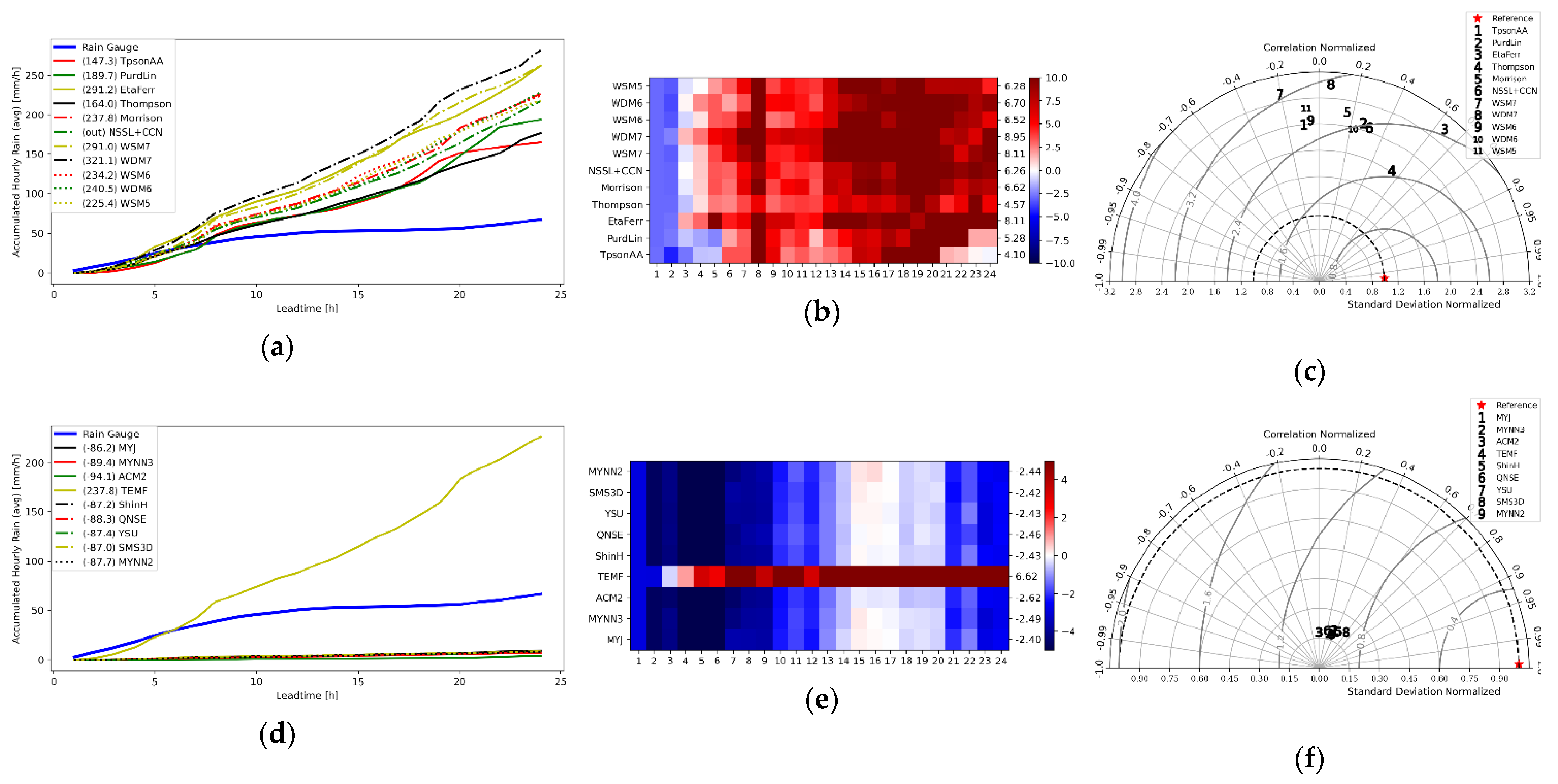
In Equations (1)–(6), x indicates any variable, f is the forecast value, and o is the observed value. The cumulative hourly rainfall values observed at the rain gauge stations were compared with the cumulative hourly rainfall values predicted on an average across the nine grid points closest to the position of the rain gauge in focus (Figure 2f). Equation (4) is used to calculate the RMS when the values σf, σo, and Rf,o are used in the normalized Taylor diagram form [57]. When some configurations showed similar results, the next set of schemes to be checked were analyzed not only with the improved configuration considered, but also with all the schemes considered good. Similarly, when the RE and the bias were close between two different configurations, the Taylor diagram was used as a tiebreaker metric.
2.5. Diagnostic Analysis
To characterize the severe rainfall events, several dynamic and thermodynamic parameters were calculated in the regions where the maximum precipitation was verified and where there were municipalities with confirmed occurrences of natural disasters (regions denoted by the yellow box). To analyze atmospheric instability and initial convection resistance, the CAPE (Equation (7)) and CINE (Equation (8)) indicators were used, respectively. The moisture supply at low levels was measured using moisture flux convergence (MFC, Equation (9)). The support at high and medium levels was verified using cyclonic vorticity advection (ADVζ, Equation (10)), disregarding the β term due to low latitudes. The relationship between vertical wind shear and the severity condition of the studied events was also verified through vertical bulk shear in the deep layer (0–6 km, Equation (11)) and the middle layer (0–3 km, Equation (12)) and the evaluation of the change in wind direction with height.
where u and v are, respectively, the zonal and meridional wind components at the corresponding levels; Rd is the specific gas constant for dry air; Tvp is the virtual temperature of a rising air parcel through the humid adiabatic; Tve is the virtual environment temperature; pf, pn, and pi are, respectively, the isobaric levels of free convection, equilibrium, and lift condensation; q and ζ are the specific humidity and the relative vorticity, respectively; CAPE, CINE, u, and v are provided by the model; and q is calculated through the vapor pressure of the air and ζ through the wind components.
3. Results
3.1. Synoptic Analysis
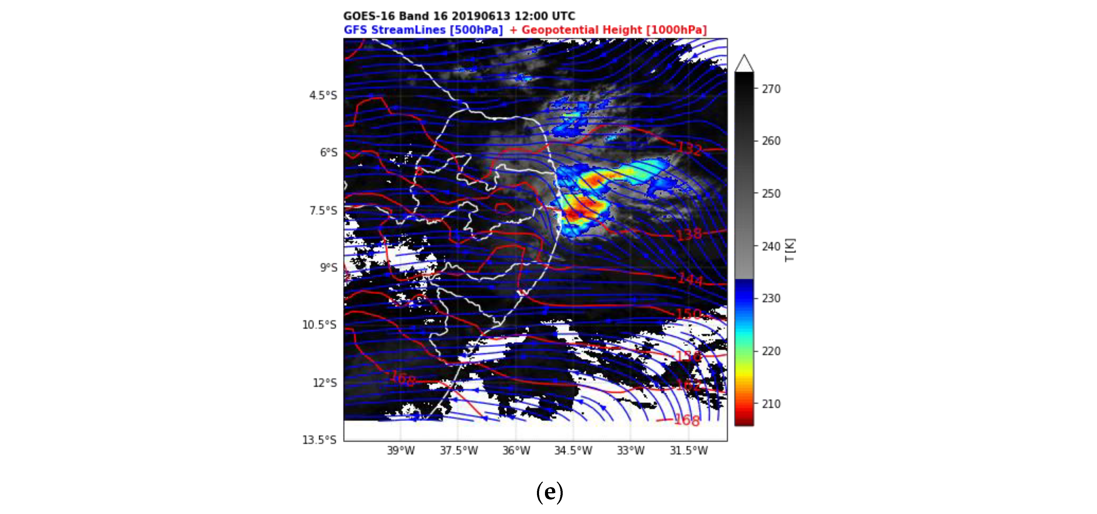
The five episodes of severe rainfall chosen for the numerical simulations were classified as (i) 20170528, a mesoscale convective system (MCS) with a trough on the surface parallel to the coast (Figure 3a); (ii) 20170720, an isolated system with less cloudiness than in the previous case, positioned to the east of a trough and favored by a confluence of high-level winds (Figure 3b); (iii) 20180422, an intense runoff embedded in pulses of ITCZ cloudiness from the northern NEB coast (Figure 3c); (iv) 20190529, an isolated storm formed due to the presence of a ridge on the east between the states of Alagoas and Pernambuco, forcing a cyclonic wind curvature near the surface (Figure 3d); and (v) 20190613, a storm formed due to a ridge in eastern Pernambuco that tilts at a height toward the coast, where convection is intense (Figure 3e).
Events 1, 2, and 5 were associated with rainfall with large spatial extents, whereas events 3 and 4 were rainfall events concentrated in smaller regions. In events 1 through 4, strong mass divergence was observed between the 850 hPa and 600 hPa levels, generally with a maximum at the 750 hPa level, on the order of 6.0 to 10.0 × 10⁻⁵ s−1. This strong divergence in the low- to mid-level layer was almost always accompanied by convergence in the lower layer, around 900 hPa, with the maximum core on the order of −7.5 to −15.0 × 10⁻⁵ s−1 (Figures not shown). Only event 5 did not show the pair strong divergence at medium levels and strong convergence at the surface.
In event 1, starting on May 26 at 20UTC, the cloudiness began to intensify on the coast and subsequently expanded inland after being stationary in the coastal area all day on May 27. At high levels, there was diffluence of air currents and the proximity of the subtropical jet stream [86]. Near the surface, there was a trough parallel to the coast and an intense convergence of moisture flow from the ocean. This event showed local and synoptic scale characteristics and weak coupling between the high troposphere and the low troposphere. The intense precipitation developed mainly locally, and the main elements for its maintenance were trough at low levels near the coast and strong wind runoff also in the low layer (Figure 3a).
For event 2, the cloudiness was more discrete compared to the previous case. A ridge between the states of Alagoas and Pernambuco with an intense temperature gradient to the north was observed. Earlier that same day, there were upper tropospheric cyclonic vortices at an altitude [87], with a core in the state of Maranhão, and an eastern periphery influencing the coast of Pernambuco with a wind diffluence zone. In the satellite images, it was possible to observe in the water vapor channel the westward advance of two cloud cores. However, no wave characteristics were observed in low or medium levels related to the position of these cores [88]. This event was characterized by the concentration of cloudiness to the east of the surface ridge, well-related to the position of maximum precipitation, and a confluence zone of high-level winds with reduced intensity compared to the previous case (Figure 3b).
For event 3, the runoff in the high levels was essentially westerly, with intense cloudiness, observed up to three days before the intense precipitation, coming from the northwest. This cloudiness was associated with the presence of the intertropical convergence zone with entirely meridional runoff at high levels and presence of widespread cloudiness and precipitation (Figure 3c).
At the beginning of event 4, there was a closed anticyclonic circulation at high levels (Figure not shown). Even after the weakening of this circulation, an isolated storm formed to the east of a small surface ridge and intense runoff perpendicular to the coast. The position of the surface moisture core, observed by the satellite image in the water vapor channel, and the ocean moisture supply coincided with the position of maximum precipitation (Figure 2d and Figure 3d).
3.2. Numerical Simulations Analysis
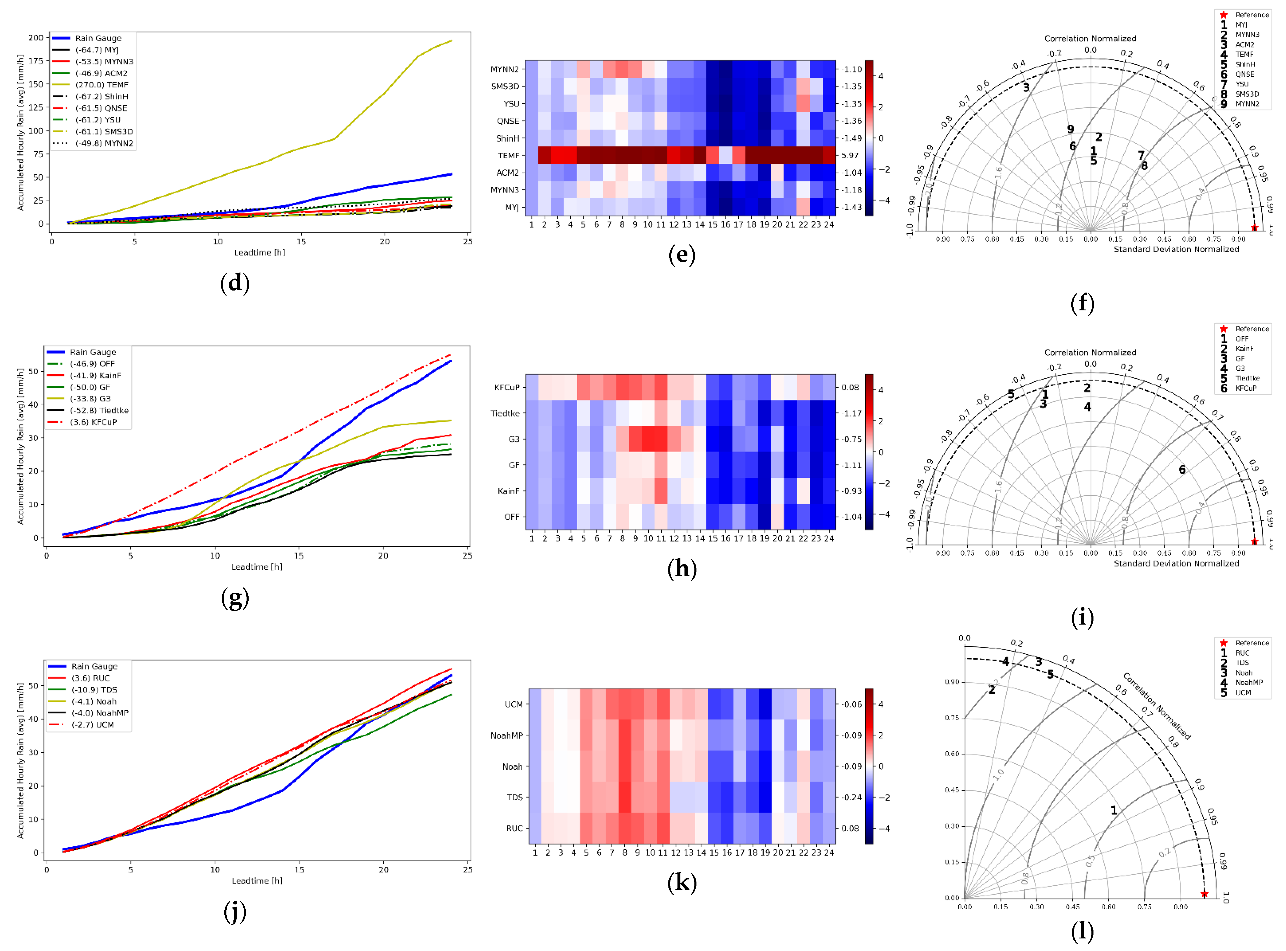
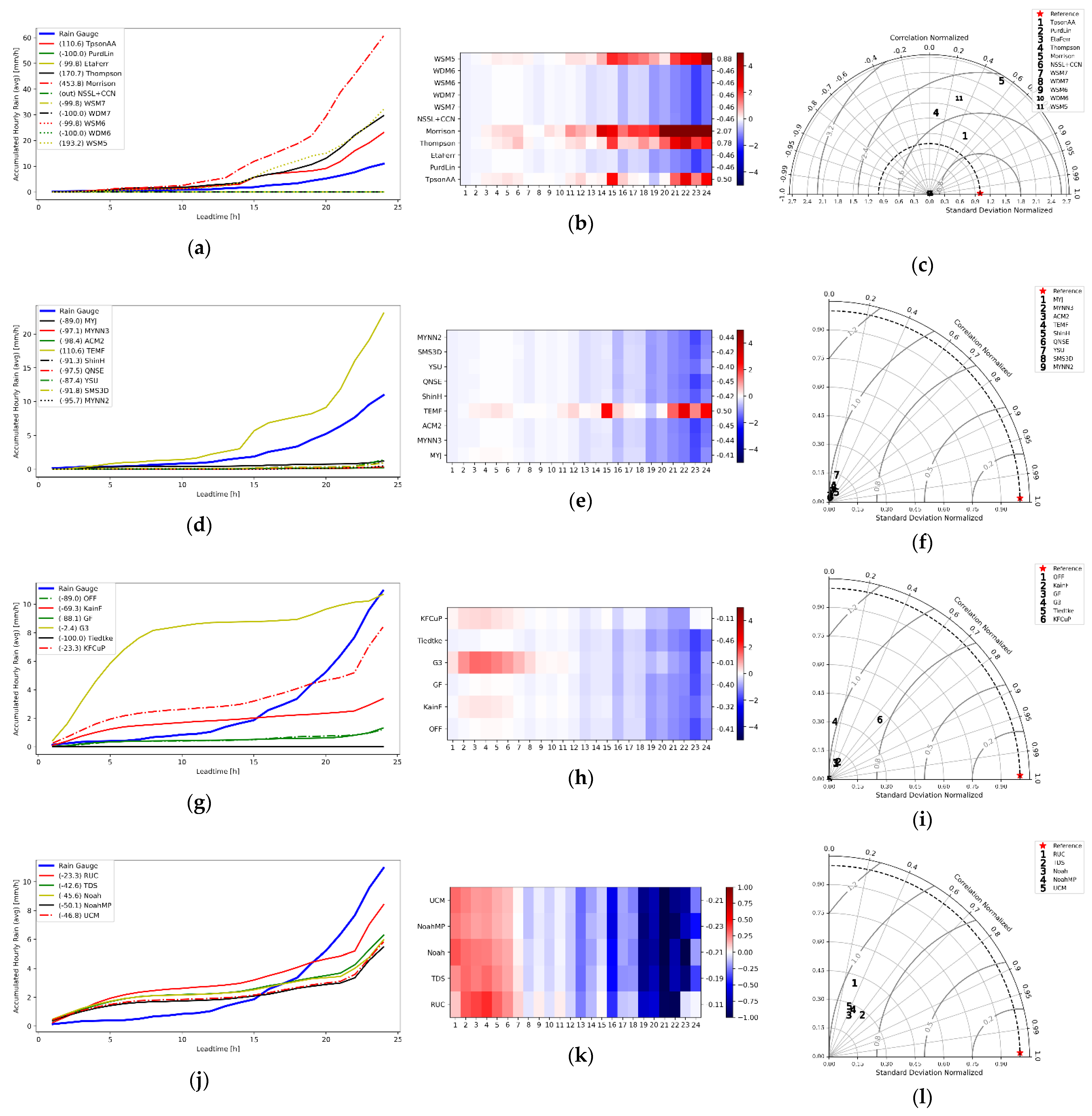
The 24-h simulation of event 1 was performed between 20170527 12UTC and 20170528 12UTC and totaled 69 runs. This event was the only one in which the best physical combinations reproduced a total average accumulation with an RE of around 50%. The Thompson and TpsonAA MPHs were the best (Figure 4a,b), with the Taylor diagram indicating Thompson first (Figure 4c). The two worst schemes were those with hail as the hydrometeor class (WSM7 and WDM7). The PBL TEMF scheme overestimated the rainfall by more than 200%, whereas the others underestimated it by around 80%. MYJ showed the best RE and the lowest bias (Figure 4d–f). Turning on the cumulus parameterization, the KainF, G3, and KFCuP schemes were able to reproduce rainfall better, with KFCuP being the best (Figure 4g–i). The RUC surface scheme showed the best RE and bias values (Figure 4j,k).
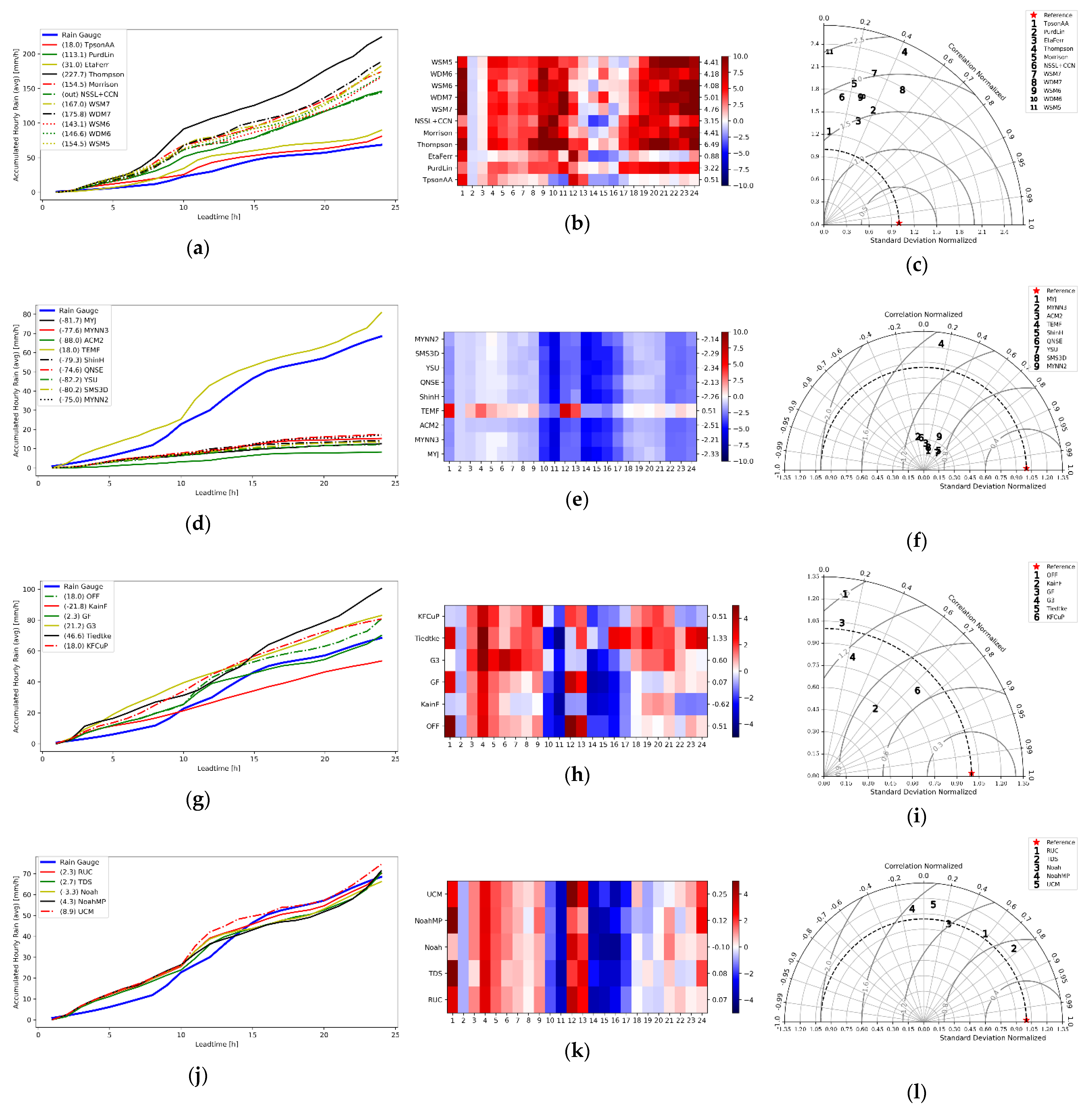
The simulations for event 2 were performed between 20170720 00UTC and 20170721 00UTC and totaled 30 runs. The three best MPHs were NSSL + CCN, EtaFerr, and TpsonAA, whereas WDM7 and WDM6 produced almost no rainfall (Figure 5a–c). For the PBL again, TEMF caused an overestimation and ACM2 was the best in terms of the RE and bias (Figure 5d–f). Again, when the cumulus parameterization was turned on, the KainF, G3, and KFCuP schemes were able to better represent the rainfall (Figure 5g–i). For the surface schemes, UCM showed better RE and bias values than RUC, but the RUC showed better values according to the Taylor diagram (Figure 5j–l).
The simulations for event 3 were performed in the period from 20180422 00UTC to 20180423 00UTC and totaled 28 runs. The best MPHs were NSSL + CCN, WDM6, and TpsonAA; and the worst, again, were WSM7 and WDM7 (Figure 6a–c). The PBL TEMF scheme continued to register overestimates, whereas ACM2 was better in all metrics (Figure 6d–f). The KainF, G3, and KFCuP schemes again showed better capability in representing rainfall, with KFCuP improving the average total period accumulations by more than 50% (Figure 6g–i). The surface physical schemes show little variation among them with the exception of RUC, which also stands out in all metrics (Figure 6j–l).
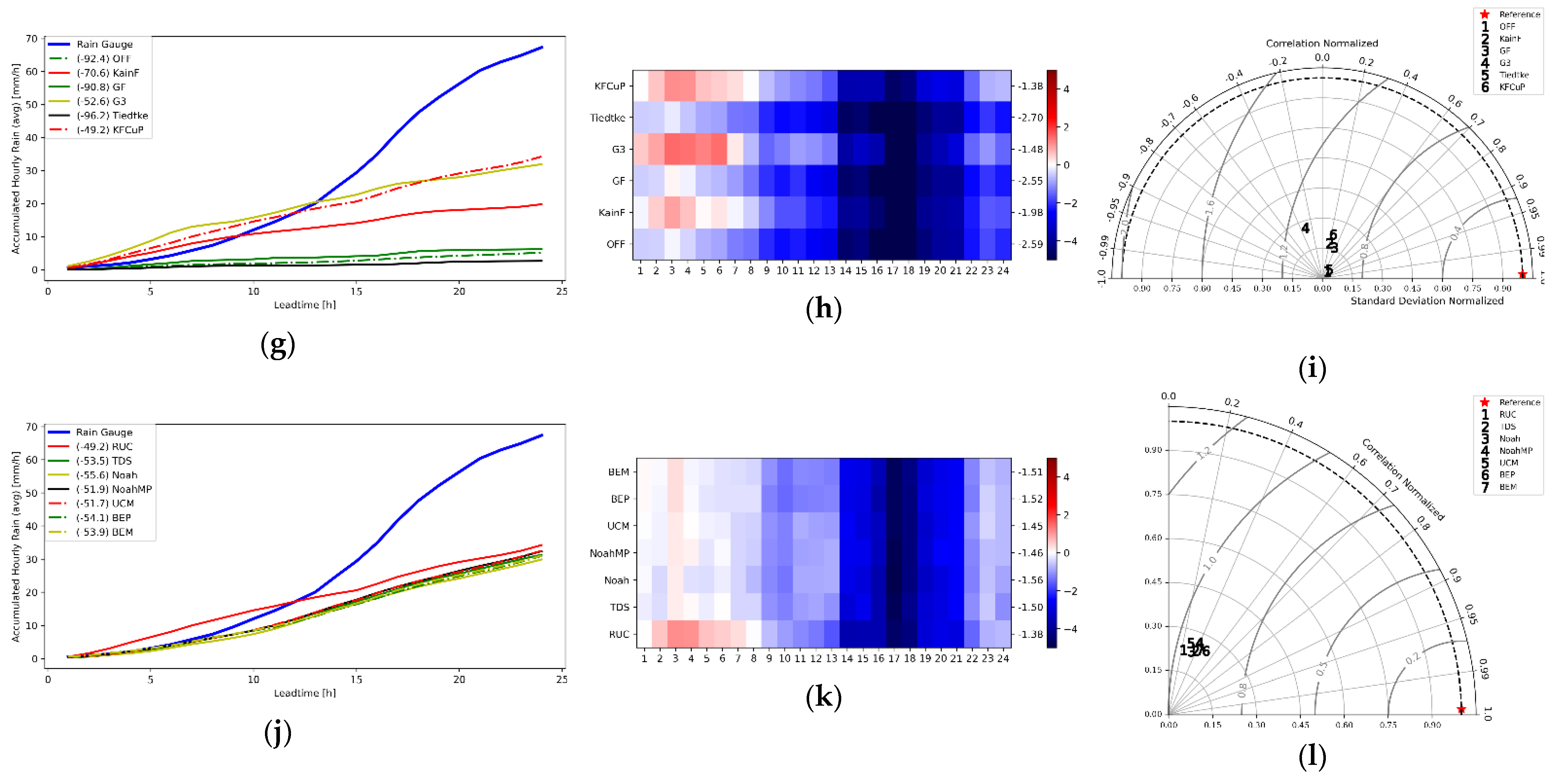
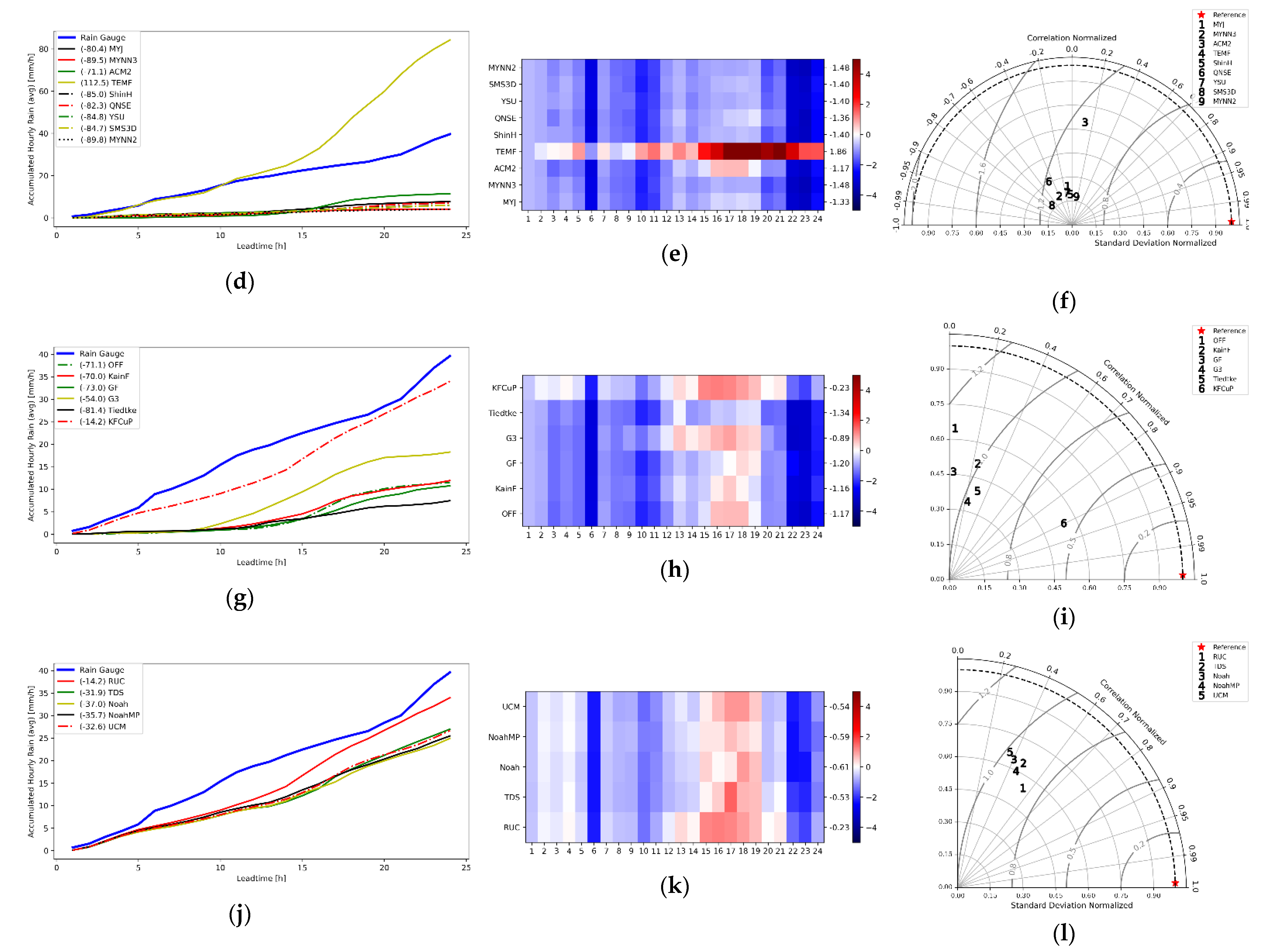
The simulations for event 4 were performed between 20190528 12UTC and 20190529 12UTC and totaled 51 runs. For the microphysics parameterizations, the schemes that were best able to represent rainfall were TpsonAA, Thompson, and WSM5. Morrison’s scheme overestimated the rainfall, and all others were barely able to generate rainfall (Figure 7a–c). The TEMF boundary layer scheme also overestimated precipitation. The MYJ and YSU schemes showed close values, with YSU being considered slightly better (Figure 7d–f). For this case, all the cumulus schemes, with the exception of Tiedtke, which failed to form rain, were able to better represent the precipitation (Figure 7g–i). The G3 parameterization showed final average rainfall accumulations close to the values measured by the rain gauges. However, it exhibits a large bias at the beginning of the simulations, making its representation in the Taylor diagram inferior to KFCuP, which was therefore chosen as the best. Again, the RUC surface scheme showed assertive displacement with respect to the others and was, therefore, chosen as the best (Figure 7j–l).
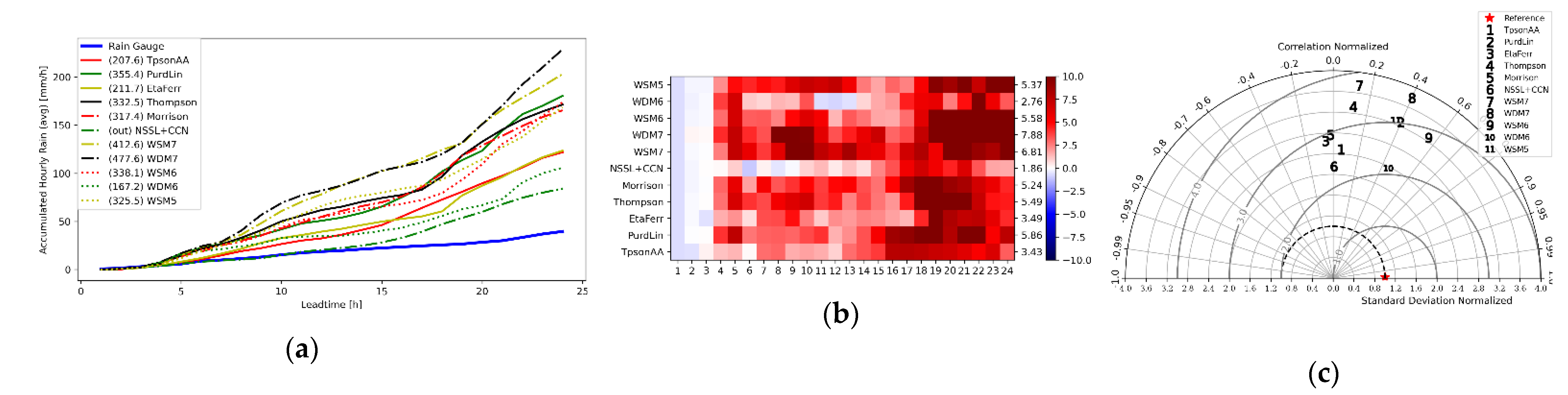
The simulations for event 5 were performed between 20190613 00UTC and 20190614 00UTC and totaled 65 runs. The microphysics schemes of NSSL + CCN and TpsonAA stood out with the best results, whereas PurdLin, WSM7, and WDM7 were the worst (Figure 8a–c). For the planetary boundary layer schemes, TEMF still overestimated, but was close to the observed values, and due to the lack of skill of the other schemes, it was the scheme that most closely matched the observed values (Figure 8d–f). The cumulus GF parameterization was the only one that was able to promote a better fit of precipitation (Figure 8g–i). For the surface schemes, RUC and TDS were the ones that stood out, with TDS chosen as the best due to the closeness of the result between the two and the better characterization of TDS by the Taylor diagram (Figure 8j–l).
3.3. Diagnostic Analysis
To describe the dynamic and thermodynamic factors that acted during the development of the storms, the atmospheric instability and the favorability of the middle and upper layers to the action of the systems were analyzed and the moisture supply in the low levels was verified with data from the best simulations obtained from the previous analyses. These analyses were performed for the regions within the yellow boxes (Figure 2a–e) for each of the events studied. Figure 9 shows the average conditions of the fluctuations of these meteorological parameters, which are the variations for event 2 and were generally considered representative of the cases analyzed.
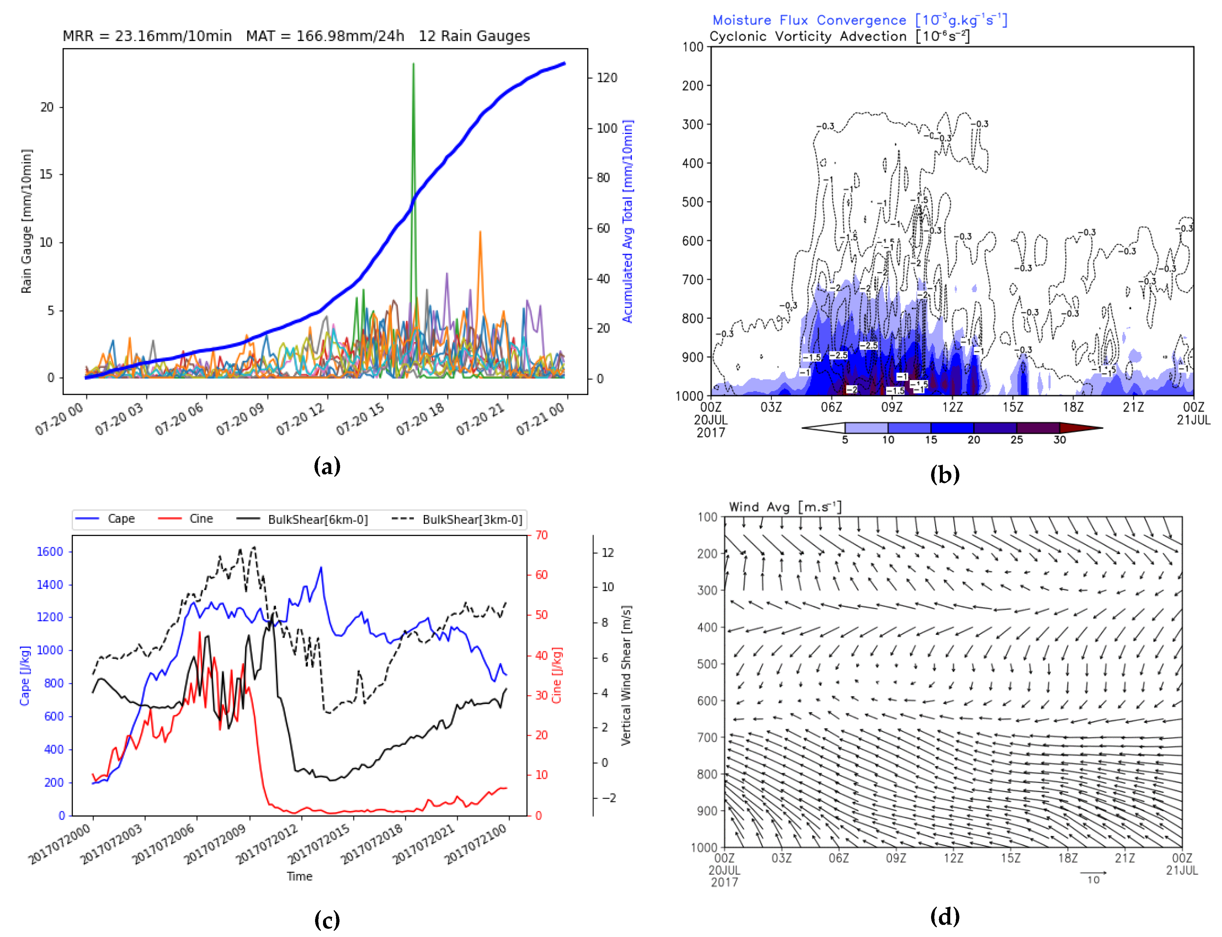
For event 2, precipitation showed an increase in intensity starting at 12UTC (Figure 9a), which was not directly related to MFC (Figure 9b). Simultaneously, there was an abrupt drop in the values of CINE and the vertical wind shear in both the deep layer and the bottom layer, accompanied by the maximum peak of the CAPE (Figure 9c). At that same instant, between the 600 hPa and 500 hPa levels, the wind weakened and the shear of its direction was remarkable (Figure 9d). In this event, a rain gauge at a certain moment registered a shower of rainfall exceeding 20 mm/10 min. The MFC reached the 700 hPa level and near-ground values on the order of 30 × 10−3 g·kg−1s−1, which was favored by an advection of cyclonic vorticity, which weakened with height and was observed until the 300 hPa level aligned with the maximum MFC values. The CAPE peaked (~1500 J·kg−1) just before the increase in precipitation intensity and CINE (~50 J·kg−1) about 3 h before the CAPE. Wind shear was the highest in the lower layer (3 km) and showed values on the order of 12 m·s−1.
For event 1, the analyses of the weather variables within the yellow box occurred in a region with a lower pluviometric density (Figure 10a). The model runs started at a time when precipitation was already being recorded, and the model was able to represent an intense MFC just after the first 3 h of simulation. Again, the MFC reached the 700 mb level, with near-surface values exceeding 30 × 10−3 g·kg−1s−1 and was well-related to cyclonic vorticity advection in the low and middle layers (Figure 10b). The CAPE values at the beginning of the storm were intense, close to 2500 J·kg−1, and after the first 6 h began to decrease in a reverse motion to the shear in the middle layer, and the CINE values began to increase (Figure 10c). In this case, increased precipitation had a direct relationship with increased wind shear in both layers.
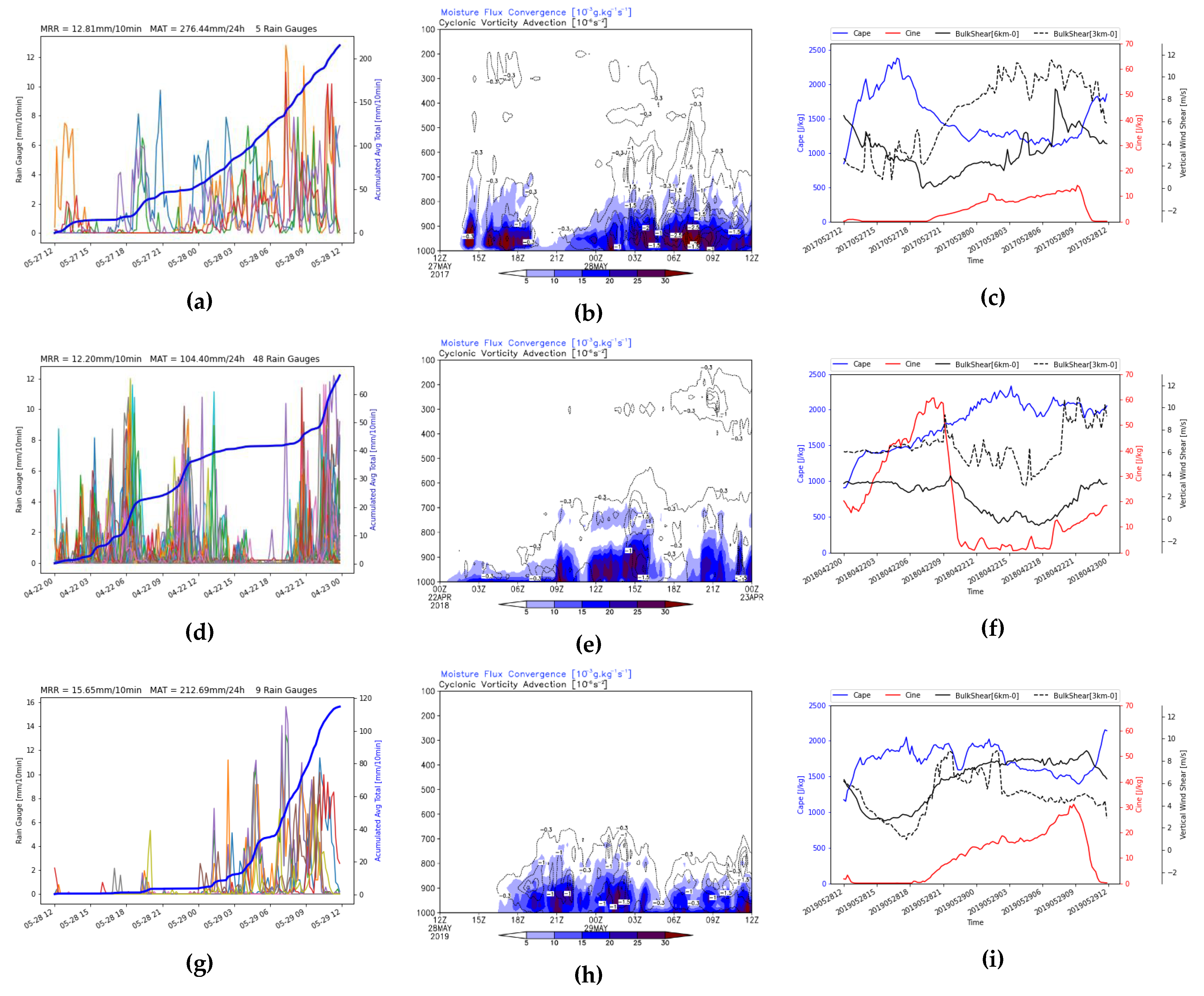
For event 3, the analyses within the yellow box covered the metropolitan region of the city of Recife that has the largest concentration of rain gauges (Figure 10d). It is possible to observe good correspondence between MFC and the precipitation peaks (Figure 10d,e). A cyclonic vorticity advection core was verified at 15 UTC between the 700 hPa and 800 hPa levels and another one at high levels at the end of the simulation and coinciding with new rainfall occurrences (Figure 10e). The inhibition energy showed rising values until around 09 UTC, when it dropped sharply, followed by a drop in wind shear values and an increase in the CAPE (Figure 10f). Again, the maximum CAPE values were near 2500 J·kg−1 and the maximum wind shear around 10 m·s−1.
Precipitation in event 4, which was a less spatially comprehensive or locally characteristic event, began effectively only after the first 12 h of simulation (Figure 10g). Despite the smaller spatial coverage, the intensity of the rainfall can be seen, with precipitation rates exceeding 15 mm/10 min. The MFC was confined to a lower layer than in the previous cases, at around 800 hPa, and the moisture supply was available at least 6 h before the onset of precipitation. No support from the medium and upper levels was observed for this event (Figure 10h). This was the only case where the shear in the deep layer was predominantly higher than the shear in the middle layer (Figure 10i). Unlike the other cases, the onset of precipitation was associated with increased CINE, maintenance of vertical shear at 6 km, and a decreased CAPE (Figure 10i). The CAPE and shear values were also lower than in the previous cases (approximately 2000 J·kg−1 and 8 m·s−1, respectively).
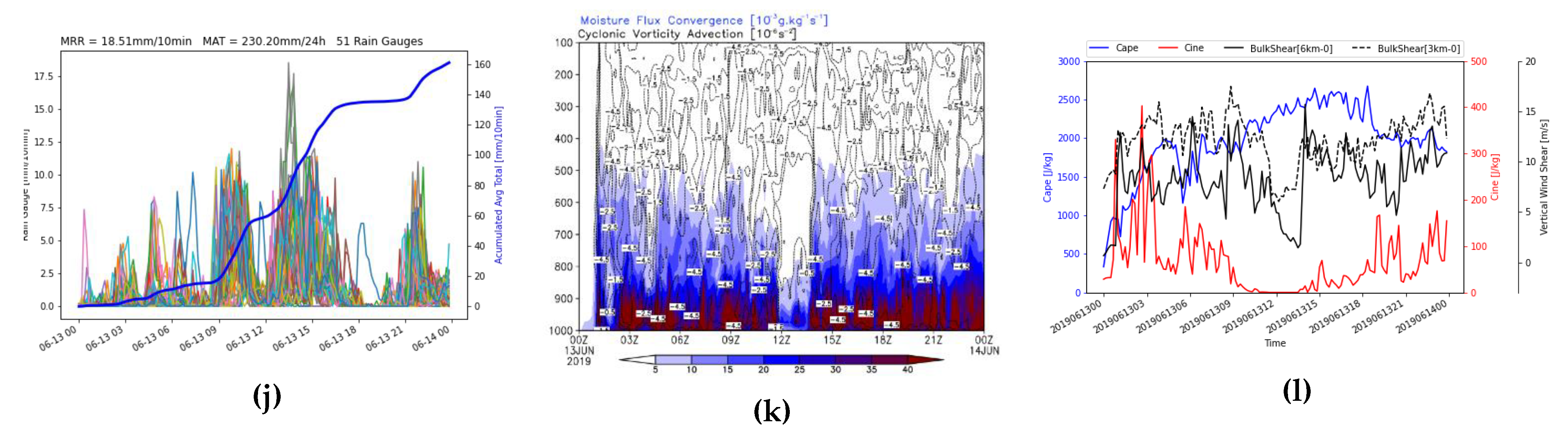
As with event 3, the analysis region for event 5 covers the metropolitan region of Recife and therefore has a larger number of rain gauges. The highest precipitation rates were greater than 18 mm/10 min (Figure 10j). This event showed the highest MFC values, over 40 × 10−3 g·kg−1s−1, also reaching the highest vertical level, around 500 hPa (Figure 10k). During the simulation strong cyclonic vorticity, advection was observed throughout the layer, with values greater than −4.5 × 10⁻⁶ s−2. Again, the CAPE reached the highest values (over 2500 J·kg−1), as did CINE at the beginning of the simulation, reaching values of 400 J·kg−1 (Figure 10l). The highest wind shear values in both layers also occurred in this case and reached values higher than 15 m·s−1. Just before the hour of maximum precipitation, falling wind shear and CINE was observed and the CAPE increased, reaching the maximum values.
4. Discussion and Conclusions
In this study, five severe rainfall events that triggered natural disasters were analyzed. Synoptic analysis showed that events 1 (20170528), 2 (20170720), 4 (20190529), and 5 (20190613) were associated with a high surface pressure, which contributed to the formation of thunderstorms to the east of its position, and with the intense trade winds that generally reach the coast perpendicularly and contribute to near-surface ocean moisture flux convergence. However, event 3 (20180422) was under the influence of ITCZ, which brought pulses of intense cloudiness from the north of the region. This analysis corroborates the results of Espinoza et al. [8] for event 1, where the contribution of the ocean moisture flux to the heavy precipitation is indicated, and also the results of Gomes et al. [88] for event 2, where it is stated that more than half of the tracked relative vorticity centers moving westward over the ocean are not classified as easterly wave disturbances. In all events, the presence of a strong wind divergence averaged over the layer between 800 hPa and 600 hPa was observed and appears to be fundamental to the occurrence of the severe thunderstorms in this region. The total rain duration in all events was greater than 24 h.
For the microphysics schemes, for all events except event 4, TpsonAA and NSSL + CCN were always in the top three. The WDM7 scheme appeared among the three worst in all cases and failed to represent any rainfall in events 2 and 4. The WSM7 microphysics also appeared among the worst three in all events except event 2. These schemes add the hail hydrometeor to the microphysical and precipitation processes. According to Bae et al. [64], these schemes tend to increase the accretion rate of ice particles due to the faster sedimentation of hail than graupel. In this way, the amount of hail is largely offset by a reduction in graupel, but it is the maximum at lower altitudes. Snow weakens the accretion of graupel at higher altitudes, which keeps it aloft, increasing its presence at medium levels. The reduction in the sum of graupel and hail in the melt layer leads to a decrease in the mixing ratio of the rain, which is compensated by falling hail. Therefore, this scheme tends to increase convective activity in regions of greater instability and decrease the intensity of precipitation in the stratiform region, thus configuring the role of hail in suppressing light precipitation and increasing heavy precipitation. This fact may have led to the poor performance of these schemes, since this region is predominantly marked by shallow warm top storms [89].
TpsonAA microphysics incorporates the activation of aerosols as cloud condensation nuclei (CCN) and ice (IN) and therefore explicitly predicts the cloud water droplet number concentration [58]. NSSL + CCN microphysics predicts the mass mixing ratio and the number of concentrations of all hydrometeor species, and the version used in this study also predicts the concentration of CCN [63,90]. It is remarkable that the best microphysics schemes verified in this study have explicit representations of aerosols and CCN. Atmospheric aerosol particles have a significant impact on the development of deep convective storms [91,92]. In a study on CCN concentration in northeastern Brazil, Almeida et al. [93] stated that the concentration of coastal aerosols is almost double the concentrations of the inland aerosols and also influences the fraction of active particles, such as CCN, which has much higher concentrations when it originates over the sea. This fact also agrees with the region of highest precipitation in event 1 (inland Figure 2a), the only case where the best microphysics was neither TpsonAA nor NSSL + CCN and was generally not well represented. Oliveira et al. [94] also analyzed aerosols in the NEB, identifying the predominant concentration of dust, marine aerosol, biomass burning, and particulate pollution, which can come from the ocean, the Amazon region, and even the coast of Africa.
For the planetary boundary layer schemes, MYJ was among the top three in three cases (being the best in event 1 and 4), ACM2 was the best in events 2 and 3, and TEMF was the best in event 5 (and the worst in all other events). The parameters relevant for severe storm prediction controlled by PBL schemes act on buoyancy through modulations in potential temperature and mixing ratio associated with stronger variability in the mixing layer depth [28]. A hypothesis for MYJ’s better performance, a 1.5-order closure local scheme, in event 1 and 4, may be related to the production of a cooler and moister PBL [95], since the region analyzed for this case was the one positioned further inland and the simulations were between 12UTC on consecutive days, which completely covers the period of greatest radiative surface cooling. In the ACM2 scheme, a first-order closure hybrid scheme, non-local mixing, is represented by a matrix that defines the mass flows between any pair of model layers even if they are not adjacent [69]. The YSU scheme, non-local first-order closure, considers the entrenchment on top of the PBL explicitly [28]. Both schemes best represent shear and buoyancy in the study by Wang et al. [96] and are generally characterized by a drying and warming daytime PBL [28]. These schemes helped in a better depiction of the rainfall in the events that occurred at the coastal zone interface (Figure 2b–d).
In the TEMF, a 1.5-order closure hybrid scheme, local mixing, is parameterized by a turbulent diffusivity, whereas the impact of non-local transport and mixing under convective conditions is parameterized using a mass flow method [70]. In events 1 through 4, this scheme overestimated the rainfall (Figure 4d, Figure 5d, Figure 6d and Figure 7d). Some works have reported a larger vertical gradient of the water vapor mixing ratio and a higher moisture content within the low cloud layer, which results in a pronounced moisture flux [70,96], which can also be verified in this study in events 1 through 4 and by the intensity of the MFC in event 5 (Figure 10k). However, in event 5, the use of this PBL scheme was crucial for a good representation of the rainfall and this was the only scheme to come close to the observed real rainfall. Wang et al. [96] further stated that no single scheme performs optimally in all aspects and that PBL schemes may depend on the atmospheric scenarios in which they are inserted. This seems to be the case for this particular event, which took place in a coastal region and was under the influence of a ridge and strong mid-level divergence. However, all these hypotheses can be more rigorously investigated by analyzing turbulent flows, diffusivity, and meteorological variables (such as potential temperature, wind, and water vapor mixing ratio) within the boundary layer, which is not within the scope of this paper.
In all events, the rain representation was better with the cumulus parameterization activated. This study was within the so-called gray zone for cumulus clouds (cumulus schemes), and several recent studies have corroborated the activation of cumulus parameterizations at resolutions between 2 to 3 km [97,98,99]. One of the main arguments for this activation is that these resolutions are still insufficient to represent the full spectrum of the convective scale [100]. The KFCuP and KainF convection schemes were better than the simulations with cumulus off in all events, whereas G3 was better than cumulus off in events 1 through 4 and GF in event 5. The innovation between KFCuP and KainF is mainly the implementation of a new trigger function related to the temperature and moisture distribution in the convective boundary layer via a probability density function [78]. To solve the problems of convective parameterizations, G3 uses ensemble and data assimilation techniques [76]. GF does a smoothing for the resolved cloud-scale transition, thus being a “scale-aware” scheme, in addition to interacting with aerosols through CCN autoconversion from cloud water to rain [75].
In all cases studied, the land surface models showed the least variation between simulations of the same event (Table 4). The RUC scheme was among the top two in all cases, and TDS was among the top two in events 3 through 5. The TDS scheme has five soil layers, and the energy budget includes radiation, sensible, and latent heat flux, whereas in this study, RUC was used with nine soil layers, taking into account water phase changes, vegetation effects, prognostic variables, and a host of features that make it much more complex [81]. The TDS scheme can be considered the simplest one currently available and performs better than the others (it was the best in event 5 and the second best in events 3 and 4). An attempt was also made to use the urban surface schemes UCM, BEM, and BEP. However, BEP and BEM were only tested in event 1 and 4 because among the PBL schemes tested in this paper, they only work with MYJ. UCM could be tested in all events, but a coherent analysis of the effects of these schemes should be restricted to, for example, the metropolitan region of Recife (within the yellow boxes in Figure 2c,e), where it is expected that these schemes can develop their characteristics and contribute to the results. Still, UCM was the second-best surface scheme with respect to the 24-h precipitation deviation in events 1 and 2. Table 4 shows the variation in the RE with respect to the average total cumulative over 24 h for each simulation set tested and the observed improvement in this same index after the best physical scheme was chosen. Disregarding the PBL TEMF scheme, the largest variations are observed when using the microphysics and cumulus schemes. When TEMF is considered, the PBL variations are as large as the microphysics ones.
In all cases, the prevailing wind at the surface and in the low layer was from the southeast and/or the east, in agreement with the action of the trade winds in the region. In all cases, the moisture flux convergence in the low layer reached the 800 hPa level. In general, MFC was well-related to precipitation, with maximum values observed before and during maximum precipitation, reaching values higher than 30 × 10−3 g·kg−1s−1 in events 1 through 4 and higher than 40 × 10−3 g·kg−1s−1 in event 5, values comparable to the occurrence of the most robust updrafts [101]. The cyclonic vorticity advection at medium and high levels supported the convergence at low levels in events 1, 2, 3, and 5. Only in event 4, considered as an isolated storm case, the support of the high and middle layers was not observed. The lowest maximum CAPE value was observed in event 2 (around 1400 J·kg−1), and the highest in event 5 (around 2500 J·kg−1). The maximum values of the CINE were between 30 and 60 J·kg−1 in events 2 through 4. In event 5, it reached about 400 J·kg−1 at the beginning of the simulation, and in event 1, it presented the lowest values, increasing throughout the simulation. As expected, the values of the CAPE and CINE show antagonistic movements, with a sharp drop in the values of CINE from the maintenance of the CAPE and/or after reaching certain values (between 1200 and 1500 J·kg−1).
The vertical wind shear in the deep layer was higher than the shear in the middle layer only in event 4. In the other events, the shear in the middle layer was higher, with maximum values between 10 and 12 m·s−1 for events 1 through 4 and at around 15 m·s−1 for event 5. An inverse relationship was also observed between the wind shear in both layers and the CAPE values, that is, after wind shear intensifies, the CAPE values tend to decrease. However, the higher precipitation rates were associated with increased wind shear, most noticeable in the deep layer for event 4 and in the middle layer for the other events. In general, the wind shear starts at values around 6 m·s−1, presents a drop after the first precipitations, and gradually increases, contributing to the maintenance of the storm’s lifetime.
Author Contributions
Conceptualization, S.B.C. and D.L.H.; methodology, S.B.C.; numerical modeling, D.O.d.S.; validation, D.L.H. and S.B.C.; formal analysis, S.B.C.; writing—original draft preparation, S.B.C.; writing—review and editing, D.L.H.; visualization, S.B.C., D.L.H., and D.O.d.S.; supervision, D.L.H.; project administration, D.L.H.; funding acquisition, D.L.H. and D.O.d.S. All authors have read and agreed to the published version of the manuscript.
Funding
Coordination of Superior Level Staff Improvement (CAPES) (Finance Code 001) and the National Council for Scientific and Technological Development (CNPq) (Process No. 400065/2014-2, Process No. 455990/2014-0 and Process No. 311473/2021-0).
Institutional Review Board Statement
Not applicable.
Informed Consent Statement
Not applicable.
Data Availability Statement
Not applicable.
Acknowledgments
We would like to thank Yannick Copin from the Institut de Physique des deux Infinis from Lyon for providing the algorithm for constructing the Taylor diagrams (https://gist.github.com/ycopin/3342888 (accessed on 10 March 2020)).
Conflicts of Interest
The authors declare no conflict of interest.
References
- de Assis Dias, M.C.; Saito, S.M.; dos Santos Alvalá, R.C.; Stenner, C.; Pinho, G.; Nobre, C.A.; de Souza Fonseca, M.R.; Santos, C.; Amadeu, P.; Silva, D.; et al. Estimation of exposed population to landslides and floods risk areas in Brazil, on an intra-urban scale. Int. J. Disaster Risk Reduct. 2018, 31, 449–459. [Google Scholar] [CrossRef]
- CEPED. Atlas Brasileiro de Desastres Naturais 1991 a 2010: Volume Brasil; CEPED UFSC: Florianópolis, Brazil, 2012; ISBN 9788564695085. [Google Scholar]
- Avelar, A.S.; Netto, A.L.C.; Lacerda, W.A.; Becker, L.B.; Mendonça, M.B. Mechanisms of the recent catastrophic landslides in the mountainous range of Rio de Janeiro, Brazil. Landslide Sci. Pract. Glob. Environ. Chang. 2013, 4, 265–270. [Google Scholar] [CrossRef]
- Luiza, A.; Netto, C.; Sato, A.M.; de Souza, A.; Vianna, L.G.G.; Araújo, I.S.; David, L.C.; Lima, P.H.; Silva, A.P.A.; Silva, R.P. Landslide Science and Practice; Springer: Berlin/Heidelberg, Germany, 2013. [Google Scholar]
- Metodiev, D.; de Andrade, M.R.M.; Mendes, R.M.; de Moraes, M.A.E.; Konig, T.; Bortolozo, C.A.; Bernardes, T.; Luiz, R.A.F.; Coelho, J.O.M. Correlation between rainfall and mass movements in North Coast Region of Sao Paulo State, Brazil for 2014–2018. Int. J. Geosci. 2018, 9, 669–679. [Google Scholar] [CrossRef] [Green Version]
- Ávila, A.; Justino, F.; Wilson, A.; Bromwich, D.; Amorim, M. Recent precipitation trends, flash floods and landslides in southern Brazil. Environ. Res. Lett. 2016, 11, 114029. [Google Scholar] [CrossRef]
- Marengo, J.A.; Espinoza, J.C. Extreme seasonal droughts and floods in Amazonia: Causes, trends and impacts. Int. J. Climatol. 2016, 36, 1033–1050. [Google Scholar] [CrossRef]
- Espinoza, N.S.; Dos Santos, C.A.C.; Silva, M.T.; Gomes, H.B.; Ferreira, R.R.; da Silva, M.L.; Santos E Silva, C.M.; de Oliveira, C.P.; Medeiros, J.; Giovannettone, J.; et al. Landslides triggered by the may 2017 extreme rainfall event in the east coast northeast of Brazil. Atmosphere 2021, 12, 1261. [Google Scholar] [CrossRef]
- Smithson, P.A. IPCC, 2001: Climate change 2001: The scientific basis. Contribution of working group 1 to the third assessment report of the intergovernmental panel on climate change, edited by J. T. Houghton, Y. Ding, D. J. Griggs, M. Noguer, P. J. van der Linden, X. Dai, K. Maskell and C. A. Johnson (eds). Cambridge University Press, Cambridge, UK, and New York, USA, 2001. No. of pages: 881. Price £34.95, US$ 49.95, ISBN 0-521-01495-6 (paperback). £90.00, US$ 130.00, ISBN 0-521-80767-0 (hardback). Int. J. Climatol. 2002, 22, 1144. [Google Scholar] [CrossRef]
- IPCC. Managing the Risks of Extreme Events and Disasters to Advance Climate Change Adaptation: Special Report of the Intergovernmental Panel on Climate Change; Field, C.B., Barros, V., Stocker, T.F., Dahe, Q., Eds.; Cambridge University Press: Cambridge, UK, 2012; ISBN 9781107025066. [Google Scholar]
- Freire, A.F.R. A Política Nacional de Proteção e Defesa Civil e as Ações do Governo Federal na Gestão de Risco de Desastres. Master’s Dissertation, Escola Nacional de Saúde Pública Sergio Arouca, Rio de Janeiro, Brazil, 2014. [Google Scholar]
- Debortoli, N.S.; Camarinha, P.I.M.; Marengo, J.A.; Rodrigues, R.R. An index of Brazil’s vulnerability to expected increases in natural flash flooding and landslide disasters in the context of climate change. Nat. Hazards 2017, 86, 557–582. [Google Scholar] [CrossRef]
- Holton, J.R.; Hakim, G.J. An Introduction to Dynamic Meteorology, 5th ed.; Elsevier Inc.: Oxford, UK, 2013. [Google Scholar]
- de Medeiros, E.S.; de Lima, R.R.; de Olinda, R.A.; dos Santos, C.A.C. Modeling spatiotemporal rainfall variability in Paraíba, Brazil. Water 2019, 11, 1843. [Google Scholar] [CrossRef] [Green Version]
- Silva, T.R.B.F.; dos Santos, C.A.C.; Silva, D.J.F.; Santos, C.A.G.; Silva, R.M.D.; Brito, J.I.B.D. Climate indices-based analysis of rainfall spatiotemporal variability in Pernambuco State, Brazil. Water 2022, 14, 2190. [Google Scholar] [CrossRef]
- Lala, J.; Bazo, J.; Anand, V.; Block, P. Optimizing forecast-based actions for extreme rainfall events. Clim. Risk Manag. 2021, 34, 100374. [Google Scholar] [CrossRef]
- Merino, A.; García-Ortega, E.; Navarro, A.; Sánchez, J.L.; Tapiador, F.J. WRF hourly evaluation for extreme precipitation events. Atmos. Res. 2022, 274, 106215. [Google Scholar] [CrossRef]
- Gebrechorkos, S.H.; Pan, M.; Beck, H.E.; Sheffield, J. Performance of state-of-the-art C3S European seasonal climate forecast models for mean and extreme precipitation over Africa. Water Resour. Res. 2022, 58, e2021WR031480. [Google Scholar] [CrossRef]
- Skamarock, W.C.; Klemp, J.B. A time-split nonhydrostatic atmospheric model for weather research and forecasting applications. J. Comput. Phys. 2008, 227, 3465–3485. [Google Scholar] [CrossRef]
- Gao, L.; Wei, J.; Lei, X.; Ma, M.; Wang, L.; Guan, X.; Lin, H. Simulation of an extreme precipitation event using ensemble-based WRF model in the Southeastern Coastal Region of China. Atmosphere 2022, 13, 194. [Google Scholar] [CrossRef]
- Herman, G.R.; Schumacher, R.S. Extreme precipitation in models: An evaluation. Weather Forecast. 2016, 31, 1853–1879. [Google Scholar] [CrossRef]
- Pereira, S.C.; Carvalho, A.C.; Ferreira, J.; Nunes, J.P.; Kaiser, J.J.; Rocha, A. Weather model performance on extreme rainfall events simulation’s over Western Iberian Peninsula. Hydrol. Earth Syst. Sci. Discuss. 2012, 9, 9163–9191. [Google Scholar] [CrossRef] [Green Version]
- Nooni, I.K.; Tan, G.; Hongming, Y.; Saidou Chaibou, A.A.; Habtemicheal, B.A.; Gnitou, G.T.; Lim Kam Sian, K.T.C. Assessing the performance of WRF Model in simulating heavy precipitation events over East Africa using satellite-based precipitation product. Remote Sens. 2022, 14, 1964. [Google Scholar] [CrossRef]
- Gettelman, A.; Rood, R.B. Demystifying Climate Models: A Users Gruide to Earth System Models, 1st ed.; Springer Open: Heidelberg, Germany, 2016; ISBN 978-3-662-48959-8. [Google Scholar]
- Jeworrek, J.; West, G.; Stull, R. WRF precipitation performance and predictability for systematically varied parameterizations over complex terrain. Weather Forecast. 2021, 36, 893–913. [Google Scholar] [CrossRef]
- Kessler, E. On the distribution and continuity of water substance in atmospheric circulations. Meteorol. Monogr. 1969, 10, 96. [Google Scholar]
- Arakawa, A. The cumulus parameterization problem: Past, present, and future. J. Clim. 2004, 17, 2493–2525. [Google Scholar] [CrossRef]
- Cohen, A.E.; Cavallo, S.M.; Coniglio, M.C.; Brooks, H.E. A review of planetary boundary layer parameterization schemes and their sensitivity in simulating southeastern U.S. cold season severe weather environments. Weather Forecast. 2015, 30, 591–612. [Google Scholar] [CrossRef]
- Hong, S.-Y.Y.; Noh, Y.; Dudhia, J. A new vertical diffusion package with an explicit treatment of entrainment processes. Mon. Weather Rev. 2006, 134, 2318–2341. [Google Scholar] [CrossRef] [Green Version]
- Wong, M.; Romine, G.; Snyder, C. Model improvement via systematic investigation of physics tendencies. Mon. Weather Rev. 2020, 148, 671–688. [Google Scholar] [CrossRef]
- Tapiador, F.J.; Tao, W.K.; Shi, J.J.; Angelis, C.F.; Martinez, M.A.; Marcos, C.; Rodriguez, A.; Hou, A. A comparison of perturbed initial conditions and multiphysics ensembles in a severe weather episode in Spain. J. Appl. Meteorol. Climatol. 2012, 51, 489–504. [Google Scholar] [CrossRef] [Green Version]
- Mahbub Alam, M. Impact of cloud microphysics and cumulus parameterization on simulation of heavy rainfall event during 7–9 October 2007 over Bangladesh. J. Earth Syst. Sci. 2014, 123, 259–279. [Google Scholar] [CrossRef] [Green Version]
- Jeworrek, J.; West, G.; Stull, R. Evaluation of cumulus and microphysics parameterizations in WRF across the convective gray zone. Weather Forecast. 2019, 34, 1097–1115. [Google Scholar] [CrossRef]
- Lu, J.; Feng, T.; Li, J.; Cai, Z.; Xu, X.; Li, L.; Li, J. Impact of assimilating Himawari-8-derived layered precipitable water with varying cumulus and microphysics parameterization schemes on the simulation of Typhoon Hato. J. Geophys. Res. Atmos. 2019, 124, 3050–3071. [Google Scholar] [CrossRef]
- On, N.; Kim, H.M.; Kim, S. Effects of resolution, cumulus parameterization scheme, and probability forecasting on precipitation forecasts in a high-resolution limited-area ensemble prediction system. Asia-Pacific J. Atmos. Sci. 2018, 54, 623–637. [Google Scholar] [CrossRef]
- Gao, Y.; Leung, L.R.; Zhao, C.; Hagos, S. Sensitivity of U.S. summer precipitation to model resolution and convective parameterizations across gray zone resolutions. J. Geophys. Res. Atmos. 2017, 122, 2714–2733. [Google Scholar] [CrossRef]
- Wagner, A.; Heinzeller, D.; Wagner, S.; Rummler, T.; Kunstmann, H. Explicit convection and scale-aware cumulus parameterizations: High-resolution simulations over areas of different topography in Germany. Mon. Weather Rev. 2018, 146, 1925–1944. [Google Scholar] [CrossRef]
- Jia, W.; Zhang, X. The role of the planetary boundary layer parameterization schemes on the meteorological and aerosol pollution simulations: A review. Atmos. Res. 2020, 239, 104890. [Google Scholar] [CrossRef]
- Falasca, S.; Gandolfi, I.; Argentini, S.; Barnaba, F.; Casasanta, G.; Di Liberto, L.; Petenko, I.; Curci, G. Sensitivity of near-surface meteorology to PBL schemes in WRF simulations in a port-industrial area with complex terrain. Atmos. Res. 2021, 264, 105824. [Google Scholar] [CrossRef]
- He, J.J.; Yu, Y.; Yu, L.J.; Liu, N.; Zhao, S.P. Impacts of uncertainty in land surface information on simulated surface temperature and precipitation over China. Int. J. Climatol. 2017, 37, 829–847. [Google Scholar] [CrossRef]
- López-Bravo, C.; Caetano, E.; Magaña, V. Forecasting summertime surface temperature and precipitation in the Mexico city metropolitan area: Sensitivity of the wrf model to land cover changes. Front. Earth Sci. 2018, 6, 6. [Google Scholar] [CrossRef] [Green Version]
- Stensrud, D.J.; Ming, X.; Wicker, L.J.; Kelleher, K.E.; Foster, M.P.; Schaefer, J.T.; Schneider, R.S.; Benjamin, S.G.; Weygandt, S.S.; Ferree, J.T.; et al. Convective-scale warn-on-forecast system: A vision for 2020. Bull. Am. Meteorol. Soc. 2009, 90, 1487–1499. [Google Scholar] [CrossRef]
- Jorgensen, A.P.; Weckwerth, T.M. Forcing and organization of convective systems. In Radar and Atmospheric Science: A Collection of Essays in Honor of David Atlas; American Meteorological Society: Boston, MA, USA, 2003; pp. 75–104. ISBN 78-1-878220-36-3. [Google Scholar]
- Taszarek, M.; Allen, J.T.; Brooks, H.E.; Pilguj, N.; Czernecki, B. Environments in a warming climate. Bull. Am. Meteorol. Soc. 2021, 102, 296–322. [Google Scholar] [CrossRef]
- Westermayer, A.T.; Groenemeijer, P.; Pistotnik, G.; Sausen, R.; Faust, E. Identification of favorable environments for thunderstorms in reanalysis data. Meteorol. Zeitschrift 2017, 26, 59–70. [Google Scholar] [CrossRef]
- Sherburn, K.D.; Parker, M.D. Climatology and ingredients of significant severe convection in high-shear, low-CAPE environments. Weather Forecast. 2014, 29, 854–877. [Google Scholar] [CrossRef]
- Poletti, M.L.; Parodi, A.; Turato, B. Severe hydrometeorological events in Liguria region: Calibration and validation of a meteorological indices-based forecasting operational tool. Meteorol. Appl. 2017, 24, 560–570. [Google Scholar] [CrossRef] [Green Version]
- Fabry, F. Radar Meteorology: Principles and Practice, 1st ed.; Cambridge University Press: Cambridge, UK, 2015; ISBN 978-1-107-07046-2. [Google Scholar]
- Alvares, C.A.; Stape, J.L.; Sentelhas, P.C.; de Moraes Gonçalves, J.L.; Sparovek, G. Köppen’s climate classification map for Brazil. Meteorol. Zeitschrift 2013, 22, 711–728. [Google Scholar] [CrossRef]
- CENAD. Anuário Brasileiro de Desastres Naturais 2011. Cent. Nac. Gerenciamento Riscos e Desastr. 2012, 1–82. Available online: https://antigo.mdr.gov.br/images/stories/ArquivosDefesaCivil/ArquivosPDF/publicacoes/Anuario-de-Desastres-Naturais-2011.pdf (accessed on 16 August 2022).
- CNM. Danos e prejuízos causados por desastres no Brasil entre 2013 a 2022. Confed. Nac. Municípios 2022, 1–18. Available online: https://www.cnm.org.br/biblioteca/download/15317 (accessed on 16 August 2022).
- CEMADEN. Anuário da Sala de Situação do Cemaden 2017. Cent. Nac. Monit. E Alertas Desastr. Nat. 2019, 1–51. Available online: http://www2.cemaden.gov.br/wp-content/uploads/2020/06/Anuario_Sala_Situa%C3%A7%C3%A3o_2017.pdf (accessed on 16 August 2022).
- Instituto Brasileiro de Geografia e Estatística (IBGE). População em áreas de risco no Brasil; Rio de Janeiro, Brasil, 2018. Available online: https://biblioteca.ibge.gov.br/visualizacao/livros/liv101589.pdf (accessed on 16 August 2022).
- De Assis Dias, M.C.; Saito, S.M.; dos Santos Alvalá, R.C.; Seluchi, M.E.; Bernardes, T.; Camarinha, P.I.M.; Stenner, C.; Nobre, C.A. Vulnerability index related to populations at-risk for landslides in the Brazilian Early Warning System (BEWS). Int. J. Disaster Risk Reduct. 2020, 49, 101742. [Google Scholar] [CrossRef]
- Dai, D.; Chen, L.; Ma, Z.; Xu, Z. Evaluation of the WRF physics ensemble using a multivariable integrated evaluation approach over the Haihe river basin in northern China. Clim. Dyn. 2021, 57, 557–575. [Google Scholar] [CrossRef]
- Stergiou, I.; Tagaris, E.; Sotiropoulou, R.-E.P. Sensitivity assessment of WRF parameterizations over Europe. Proceedings 2017, 1, 119. [Google Scholar] [CrossRef] [Green Version]
- Taylor, K.E. Summarizing multiple aspects of model performance in a single diagram. J. Geophys. Res. 2001, 106, 7183–7192. [Google Scholar] [CrossRef]
- Thompson, G.; Eidhammer, T. A study of aerosol impacts on clouds and precipitation development in a large winter cyclone. J. Atmos. Sci. 2014, 71, 3636–3658. [Google Scholar] [CrossRef]
- Chen, S.H.; Sun, W.Y. A one-dimensional time dependent cloud model. J. Meteorol. Soc. Japan. Ser. II 2002, 80, 99–118. [Google Scholar] [CrossRef] [Green Version]
- Rogers, E.; Black, T.; Ferrier, B.; Lin, Y.; Parrish, D.; Dimego, G. Changes to the NCEP Meso Eta Analysis and Forecast System: Increase in Resolution, New Cloud Microphysics, Modified Precipitation Assimilation, Modified 3DVAR Analysis. Available online: https://www.emc.ncep.noaa.gov/users/mesoimpldocs/mesoimpl/eta12tpb/ (accessed on 16 August 2022).
- Thompson, G.; Field, P.R.; Rasmussen, R.M.; Hall, W.D. Explicit forecasts of winter precipitation using an improved bulk microphysics scheme. Part II: Implementation of a new snow parameterization. Mon. Weather Rev. 2008, 136, 5095–5115. [Google Scholar] [CrossRef]
- Morrison, H.; Thompson, G.; Tatarskii, V. Impact of cloud microphysics on the development of trailing stratiform precipitation in a simulated squall line: Comparison of one- and two-moment schemes. Mon. Weather Rev. 2009, 137, 991–1007. [Google Scholar] [CrossRef] [Green Version]
- Mansell, E.R.; Ziegler, C.L.; Bruning, E.C. Simulated electrification of a small thunderstorm with two-moment bulk microphysics. J. Atmos. Sci. 2010, 67, 171–194. [Google Scholar] [CrossRef]
- Bae, S.Y.; Hong, S.Y.; Tao, W.K. Development of a single-moment cloud microphysics scheme with prognostic hail for the Weather Research and Forecasting (WRF) model. Asia-Pacific J. Atmos. Sci. 2019, 55, 233–245. [Google Scholar] [CrossRef]
- Hong, S.Y.; Lim, J.-O.J. The WRF single-moment 6-class microphysics scheme (WSM6). Asia-Pacific J. Atmos. Sci. 2006, 42, 129–151. [Google Scholar]
- Lim, K.S.S.; Hong, S.Y. Development of an effective double-moment cloud microphysics scheme with prognostic Cloud Condensation Nuclei (CCN) for weather and climate models. Mon. Weather Rev. 2010, 138, 1587–1612. [Google Scholar] [CrossRef] [Green Version]
- Janjić, Z.I. The step-mountain eta coordinate model: Further developments of the convection, viscous sublayer, and turbulence closure schemes. Mon. Weather Rev. 1994, 122, 927–945. [Google Scholar] [CrossRef]
- Nakanishi, M.; Niino, H. Development of an improved turbulence closure model for the atmospheric boundary layer. J. Meteorol. Soc. Japan. Ser. II 2009, 87, 895–912. [Google Scholar] [CrossRef] [Green Version]
- Pleim, J.E. A combined local and nonlocal closure model for the atmospheric boundary layer. Part I: Model description and testing. J. Appl. Meteorol. Climatol. 2007, 46, 1383–1395. [Google Scholar] [CrossRef]
- Angevine, W.M.; Jiang, H.; Mauritsen, T. Performance of an Eddy diffusivity-mass flux scheme for shallow cumulus boundary layers. Mon. Weather Rev. 2010, 138, 2895–2912. [Google Scholar] [CrossRef] [Green Version]
- Shin, H.H.; Hong, S.Y. Representation of the subgrid-scale turbulent transport in convective boundary layers at gray-zone resolutions. Mon. Weather Rev. 2015, 143, 250–271. [Google Scholar] [CrossRef]
- Sukoriansky, S.; Galperin, B.; Perov, V. ‘Application of a New Spectral Theory of stably stratified turbulence to the atmospheric boundary layer over Sea Ice. ’ Bound. Layer Meteorol. 2005, 117, 231–257. [Google Scholar] [CrossRef]
- Zhang, X.; Bao, J.W.; Chen, B.; Grell, E.D. A three-dimensional scale-adaptive turbulent kinetic energy scheme in the WRF-ARW model. Mon. Weather Rev. 2018, 146, 2023–2045. [Google Scholar] [CrossRef]
- Kain, J.S. The Kain–Fritsch convective parameterization: An update. J. Appl. Meteorol. Climatol. 2004, 43, 170–181. [Google Scholar] [CrossRef]
- Grell, G.A.; Freitas, S.R. A scale and aerosol aware convective parameterization for weather and air quality modeling. Atmos. Chem. Phys. 2013, 13, 23845–23893. [Google Scholar] [CrossRef]
- Grell, G.A.; Dévényi, D. A generalized approach to parameterizing convection combining ensemble and data assimilation techniques. Geophys. Res. Lett. 2002, 29, 38-1-38-4. [Google Scholar] [CrossRef] [Green Version]
- Zhang, C.; Wang, Y.; Hamilton, K. Improved representation of boundary layer clouds over the Southeast Pacific in ARW-WRF using a modified Tiedtke Cumulus parameterization scheme. Mon. Weather Rev. 2011, 139, 3489–3513. [Google Scholar] [CrossRef] [Green Version]
- Berg, L.K.; Gustafson, W.I.; Kassianov, E.I.; Deng, L. Evaluation of a modified scheme for shallow convection: Implementation of CuP and case studies. Mon. Weather Rev. 2013, 141, 134–147. [Google Scholar] [CrossRef]
- Dudhia, J. A multi-layer soil temperature model for MM5. In Proceedings of the Sixth PSU/NCAR Mesoscale Model Users’ Workshop, Boulder, CO, USA, 22–24 July 1996. [Google Scholar]
- Tewari, M.; Chen, F.; Wang, W.; Dudhia, J.; LeMone, M.A.; Mitchell, K.; Ek, M.; Gayno, G.; Wegiel, J.; Cuenca, R.H. Implementation and verification of the unified NOAH land surface model in the WRF model. In Proceedings of the 20th Conference on Weather Analysis and Forecasting/16th conference on numerical weather prediction, Seattle, WA, USA, 14 January 2004; pp. 11–15. [Google Scholar]
- Benjamin, S.G.; Grell, G.A.; Brown, J.M.; Smirnova, T.G.; Bleck, R. Mesoscale weather prediction with the RUC hybrid isentropic–terrain-following coordinate model. Mon. Weather Rev. 2004, 132, 473–494. [Google Scholar] [CrossRef]
- Niu, G.Y.; Yang, Z.L.; Mitchell, K.E.; Chen, F.; Ek, M.B.; Barlage, M.; Kumar, A.; Manning, K.; Niyogi, D.; Rosero, E.; et al. The community Noah land surface model with multiparameterization options (Noah-MP): 1. Model description and evaluation with local-scale measurements. J. Geophys. Res. Atmos. 2011, 116, 12109. [Google Scholar] [CrossRef] [Green Version]
- Chen, F.; Kusaka, H.; Bornstein, R.; Ching, J.; Grimmond, C.S.B.; Grossman-Clarke, S.; Loridan, T.; Manning, K.W.; Martilli, A.; Miao, S.; et al. The integrated WRF/urban modelling system: Development, evaluation, and applications to urban environmental problems. Int. J. Climatol. 2011, 31, 273–288. [Google Scholar] [CrossRef]
- Salamanca, F.; Martilli, A. A new building energy model coupled with an urban canopy parameterization for urban climate simulations-part II. Validation with one dimension off-line simulations. Theor. Appl. Climatol. 2010, 99, 345–356. [Google Scholar] [CrossRef]
- Martilli, A.; Clappier, A.; Rotach, M.W. An urban surface exchange parameterisation for mesoscale models. Bound. Layer Meteorol. 2002, 104, 261–304. [Google Scholar] [CrossRef]
- Fedorova, N.; Levit, V.; Campos, A.M.V. Brazilian Northeast jet stream: Association with synoptic-scale systems. Meteorol. Appl. 2018, 25, 261–268. [Google Scholar] [CrossRef] [Green Version]
- de Morais, M.D.C.; Gan, M.A.; Yoshida, M.C. Features of the upper tropospheric cyclonic vortices of Northeast Brazil in life cycle stages. Int. J. Climatol. 2021, 41, E39–E58. [Google Scholar] [CrossRef]
- Gomes, H.B.; Ambrizzi, T.; Herdies, D.L.; Hodges, K.; Pontes Da Silva, B.F. Easterly wave disturbances over Northeast Brazil: An observational analysis. Adv. Meteorol. 2015, 2015, 176238. [Google Scholar] [CrossRef] [Green Version]
- Araújo Palharini, R.S.; Vila, D.A. Climatological behavior of precipitating clouds in the northeast region of Brazil. Adv. Meteorol. 2017, 2017, 5916150. [Google Scholar] [CrossRef] [Green Version]
- Li, X.; Zhang, Q.; Xue, H. The role of initial cloud condensation nuclei concentration in hail using the WRF NSSL 2-moment microphysics scheme. Adv. Atmos. Sci. 2017, 34, 1106–1120. [Google Scholar] [CrossRef]
- Sun, J.; Ariya, P.A. Atmospheric organic and bio-aerosols as cloud condensation nuclei (CCN): A review. Atmos. Environ. 2006, 40, 795–820. [Google Scholar] [CrossRef]
- Hazra, A.; Chaudhari, H.S.; Ranalkar, M.; Chen, J.P. Role of interactions between cloud microphysics, dynamics and aerosol in the heavy rainfall event of June 2013 over Uttarakhand, India. Q. J. R. Meteorol. Soc. 2017, 143, 986–998. [Google Scholar] [CrossRef]
- Almeida, G.P.; Borrmann, S.; Leal Junior, J.B.V. Cloud condensation nuclei (Ccn) concentration in the brazilian northeast semi-arid region: The influence of local circulation. Meteorol. Atmos. Phys. 2014, 125, 159–176. [Google Scholar] [CrossRef]
- de Oliveira, A.M.; Souza, C.T.; de Oliveira, N.P.M.; Melo, A.K.S.; Lopes, F.J.S.; Landulfo, E.; Elbern, H.; Hoelzemann, J.J. Analysis of atmospheric aerosol optical properties in the Northeast Brazilian atmosphere with remote sensing data from MODIS and CALIOP/CALIPSO satellites, AERONET photometers and a ground-based lidar. Atmosphere 2019, 10, 594. [Google Scholar] [CrossRef] [Green Version]
- Hu, X.M.; Nielsen-Gammon, J.W.; Zhang, F. Evaluation of three planetary boundary layer schemes in the WRF model. J. Appl. Meteorol. Climatol. 2010, 49, 1831–1844. [Google Scholar] [CrossRef] [Green Version]
- Wang, W.; Shen, X.; Huang, W. A Comparison of boundary-layer characteristics simulated using different parametrization schemes. Bound. Layer Meteorol. 2016, 161, 375–403. [Google Scholar] [CrossRef]
- Mu, Z.; Zhou, Y.; Peng, L.; He, Y. Numerical rainfall simulation of different WRF parameterization schemes with different spatiotemporal rainfall evenness levels in the Ili region. Water 2019, 11, 2569. [Google Scholar] [CrossRef]
- Liu, Y.; Cheng, A.; Hu, H. Precipitation simulation from the cumulus convection parameterization schemes based on the WRF model in the Weihe River Basin, China. J. Phys. Conf. Ser. 2021, 2006, 012004. [Google Scholar] [CrossRef]
- Kotroni, V.; Lagouvardos, K. Evaluation of MM5 high-resolution real-time forecasts over the urban area of Athens, Greece. J. Appl. Meteorol. Climatol. 2004, 43, 1666–1678. [Google Scholar] [CrossRef]
- Bryan, G.H.; Wyngaard, J.C.; Fritsch, J.M. Resolution requirements for the simulation of deep moist convection. Mon. Weather Rev. 2003, 131, 2394–2416. [Google Scholar] [CrossRef]
- Banacos, P.C.; Schultz, D.M. The use of moisture flux convergence in forecasting convective initiation: Historical and operational perspectives. Weather Forecast. 2005, 20, 351–366. [Google Scholar] [CrossRef]
Figure 1.
(a) Koppen’s climate classification for the nine states of NEB (BA—Bahia, SE—Sergipe, AL—Alagoas, PE—Pernambuco, PB—Paraíba, RN—Rio Grande do Norte, CE—Ceará, PI—Piauí, and MA—Maranhão); the black rectangle is the region where the numerical simulations were performed using the WRF model. (b) A zoom-in representation of the eastern Pernambuco state; the red stars are the 298 rainfall stations used in the verification of the simulations. (c) The 28 monitored municipalities affected by natural disasters in this study (1—Recife, 2—Rio Formoso, 3—Olinda, 4—Camaragibe, 5—São Lourenço da Mata, 6—Jaboatão dos Guararapes, 7—Abreu e Lima, 8—Barreiros, 9—Caruaru, 10—Cortês, 11—Barra de Guabiraba, 12—Chã Grande, 13—Palmares, 14—Amaraji, 15—Gameleira, 16—Ribeirão, 17—Belém de Maria, 18—São Benedito do Sul, 19—Jaqueira, 20—Catende, 21—Sirinhaém, 22—Escada, 23—Primavera, 24—Ipojuca, 25—Cabo de Santo Agostinho, 26—Moreno, 27—Vitória de Santo Antão, and 28—Igarassu).

Figure 2.
The blue shading (a–e) is the 24-h precipitation accumulation (mm/24 h) recorded by the rain gauges and interpolated using the Cressman technique with a 15 km radius. (a) Precipitation ranges from 20170527 12UTC to 20170528 12UTC, (b) from 20170720 00UTC to 20170721 00UTC, (c) from 20180422 00UTC to 20180423 00UTC, (d) from 20190528 12UTC to 20190529 12UTC, and (e) from 20190613 00UTC to 20190614 00UTC. The dotted line in black marks the 100 mm/24 h isohyet, the red areas are the municipalities affected by natural disasters, and the yellow boxes are the intersection regions between the heaviest rainfall and the municipalities affected by natural disasters and where the diagnostic analyses were performed. (f) Schematic sketch with the position of a rain gauge (blue triangle) and the nine grid points used to calculate the average rainfall (red points).

Figure 3.
Synoptic and mesoscale analysis of simulated severe rainfall events: (a) satellite image on the enhanced infrared channel (13.3 µ) with isobars on the surface in red, (b) satellite image on the enhanced water vapor channel (7.4 µ), streamlines at 200 hPa, and geopotential height at 1000 hPa in red, (c) satellite image on the enhanced infrared channel (13.3 µ) and streamlines at 200 hPa, (d) satellite image on the enhanced water vapor channel (7.4 µ), streamlines at 1000 hPa, and perturbed geopotential height at 1000 hPa in red, and (e) satellite image on the enhanced infrared channel (13.3 µ), streamlines at 500 hPa in blue, and geopotential height at 1000 hPa in red.


Figure 4.
Analysis of the model settings for event 1: (a–c) microphysics settings, (d–f) the planetary boundary layer, (g–i) cumulus, and (j–l) surface parameterizations. The column on the left compares the average hourly accumulated rainfall at the rain gauges with the rainfall generated by the model according to the settings under analysis; inside the legend are the relative errors (REs) accumulated over 24 h for each configuration. The middle column shows the average hourly bias and on the secondary axis the average period bias. The column on the right shows the Taylor diagram.


Figure 5.
As in Figure 4 but for event 2.
Figure 5.
As in Figure 4 but for event 2.


Figure 6.
As in Figure 4 but for event 3.
Figure 6.
As in Figure 4 but for event 3.


Figure 7.
As in Figure 4 but for event 4.
Figure 7.
As in Figure 4 but for event 4.

Figure 8.
As in Figure 4 but for event 5.
Figure 8.
As in Figure 4 but for event 5.

Figure 9.
Analysis of the dynamic and thermodynamic variables inside the yellow box for event 2: (a) each rain gauge represents a different color (mm/10 min) and 24-h average accumulated precipitation in blue; MRR is for maximum rain rate, and MAT is for maximum accumulated total; (b) maximum MFC (10−3 g·kg−1s−1) and minimum ADVζ (10−6 s−2); (c) maximum values of CAPE and CIN (J·kg−1) and maximum values of bukk shear (m·s−1) in their respective layers (outer axis); and (d) vertical variation in the mean wind vector (m·s−1).

Figure 10.
As in Figure 9, but for event 1 from (a–c), for event 3 from (d–f), for event 4 from (g–i), and for event 5 from (j–l).
Figure 10.
As in Figure 9, but for event 1 from (a–c), for event 3 from (d–f), for event 4 from (g–i), and for event 5 from (j–l).


Table 1.
Characteristics of the severe rainfall events studied.
| Date | Municipalities Affected | Higher Rainfall Rates | Rain Duration (h) | Total Accumulated (mm) | ||
|---|---|---|---|---|---|---|
| mm/10 min | mm/1 h | mm/24 h | ||||
| 20170528 | 16 | 14.9 | 47.3 | 280.4 | 48 | 395.9 |
| 20170720 | 16 | 23.2 | 29.1 | 170.5 | 72 | 264.0 |
| 20180422 | 5 | 15.1 | 61.0 | 135.7 | 57 | 193.6 |
| 20190529 | 4 | 15.6 | 55.2 | 212.7 | 37 | 224.0 |
| 20190613 | 7 | 18.5 | 69.4 | 236.0 | 48 | 236.6 |
Table 3.
The best settings and their respective statistical metrics.
| Event Date | MP | PBL | CUM | SFC | RE (%) | Bias | σ | R * | RMS | ||
|---|---|---|---|---|---|---|---|---|---|---|---|
| Data | Model | Value | Norm | ||||||||
| 20170528 | Thompson | MYJ | KFCuP | RUC | −49.2 | −1.38 | 5.455 | 1.230 | 0.221 | 5.699 | 0.975 |
| 20170720 | NSSL + CCN | ACM2 | KFCuP | RUC | 3.6 | 0.08 | 3.386 | 2.445 | 0.860 | 3.842 | 0.528 |
| 20180422 | NSSL + CCN | ACM2 | KFCuP | RUC | −14.2 | −0.23 | 3.695 | 2.015 | 0.546 | 3.936 | 0.838 |
| 20190529 | TpsonAA | MYJ | KFCuP | RUC | −23.3 | −0.11 | 2.872 | 1.176 | 0.322 | 2.967 | 0.951 |
| 20190613 | NSSL + CCN | TEMF | GF | TDS | 2.7 | 0.08 | 5.691 | 6.429 | 0.774 | 8.421 | 0.727 |
Note: * Normalized values.
Table 4.
RE variation for each simulation set and per event (Δ%) and the best RE performed.
| Schemes | Event 1 | Event 2 | Event 3 | Event 4 | Event 5 | AVG | |||||
|---|---|---|---|---|---|---|---|---|---|---|---|
| ΔRE | Best | ΔRE | Best | ΔRE | Best | ΔRE | Best | ΔRE | Best | (ΔRE) | |
| MPH | 173.8 | −147.3 | −34.4 | −65.6 | 365.1 | 112.5 | 553.8 | −99.8 | 259.7 | 18.0 | 263.6 |
| PBL 1 | 7.9 | −86.2 | 20.3 | −46.9 | 18.7 | −71.1 | 9.4 | −89.0 | 13.4 | 18.0 | 13.9 |
| PBL 2 | 324.0 | 237.0 | 316.9 | 270.0 | 183.6 | 122.5 | 199.6 | 110.6 | 92.6 | 18.0 | 223.3 |
| CUM 3 | −47.0 | −49.2 | −56.4 | 3.6 | −67.2 | −14.2 | −97.6 | −2.4 | −44.3 | 2.3 | 62.5 |
| CUM 4 | −37.0 | --- | −50.5 | --- | −56.9 | --- | −86.6 | --- | 15.7 | --- | −43.1 |
| SFC | −6.4 | −49.2 | −8.2 | −2.7 | −22.8 | −14.2 | −26.8 | −2.4 | 6.6 | 2.3 | 11.5 |
Note: 1 PBL without TEMF. 2 PBL with TEMF. 3 Difference between the worst CUM and the best CUM. 4 Difference between the simulation without CUM and the best simulation with CUM.
Publisher’s Note: MDPI stays neutral with regard to jurisdictional claims in published maps and institutional affiliations. |
© 2022 by the authors. Licensee MDPI, Basel, Switzerland. This article is an open access article distributed under the terms and conditions of the Creative Commons Attribution (CC BY) license (https://creativecommons.org/licenses/by/4.0/).
Share and Cite
MDPI and ACS Style
Costa, S.B.; Herdies, D.L.; Souza, D.O.d. Extreme Precipitation Events on the East Coast of Brazil’s Northeast: Numerical and Diagnostic Analysis. Water 2022, 14, 3135. https://doi.org/10.3390/w14193135
AMA Style
Costa SB, Herdies DL, Souza DOd. Extreme Precipitation Events on the East Coast of Brazil’s Northeast: Numerical and Diagnostic Analysis. Water. 2022; 14(19):3135. https://doi.org/10.3390/w14193135
Chicago/Turabian StyleCosta, Saulo Barros, Dirceu Luís Herdies, and Diego Oliveira de Souza. 2022. "Extreme Precipitation Events on the East Coast of Brazil’s Northeast: Numerical and Diagnostic Analysis" Water 14, no. 19: 3135. https://doi.org/10.3390/w14193135
Note that from the first issue of 2016, this journal uses article numbers instead of page numbers. See further details here.