
Evaluation of Water—Energy—Food—Economy Coupling Efficiency Based on Three-Dimensional Network Data Envelopment Analysis Model


1
Business School, Hohai University, Nanjing 211100, China
2
College of Management and Economy, Tianjin University, Tianjin 300072, China
*
Author to whom correspondence should be addressed.
Water 2022, 14(19), 3133; https://doi.org/10.3390/w14193133
Submission received: 17 August 2022
/
Revised: 28 September 2022
/
Accepted: 29 September 2022
/
Published: 4 October 2022
(This article belongs to the Special Issue Decision-Making Theory and Methodology for Water, Energy and Food Security)
Abstract
:In the process of human survival and sustainable development, water security, energy security and food security have become the three most prominent issues, but they are interrelated and directly affect each other, that is, to form a Water–Energy–Food (WEF) nexus. Scientific understanding and correct response to the relationship between WEF is important to realize the sustainable development of natural resources. There are some deficiencies in the existing research on the input–output efficiency of WEF system. There are few articles that can study the efficiency relationship between internal and external factors (such as the economy and environment) of the WEF system at the same time, or the research is not perfect. In view of the shortcomings of the existing research, this paper establishes a three-dimensional network structure to describe the water–energy–food–economy (WEF-Eco) system and establishes the corresponding network Data Envelopment Analysis (DEA) model. We use the data of 19 provinces in Northeast, East, and central China to show the application results of this model.
1. Introduction
Food production and agricultural development are inseparable from water resources and energy. Energy development also depends on the development of water resources and the food industry to a great extent. At the same time, the development and utilization of water resources need the support of energy and food. Any one of these three resources is affected by the other two resources. For example, the low reserves of oil, natural gas, coal, and other major energy resources in the Yangtze River Economic Belt basin; the decline in water quality in several water sources; and the serious degradation of ecological functions in the basin have gradually become important factors restricting the agricultural and economic sustainability of the region. If any one of these resources is short, the fragile balance between the three will be destroyed, which will lead to serious consequences. Especially in the context of global COVID-19 intensification, population growth, environmental degradation, and intensified impacts of climate change, the problem of resource shortage has had a major impact on global development. It is important to study the internal relationship and interaction between water–energy–food (WEF) [1].
Research on WEF mainly focuses on two aspects: (1) qualitative research, including elaborating the relationship between the internal WEF system or the relationship between the WEF system and external factors such as economy and environment [2,3,4,5,6,7], determining the boundary and core issues of the WEF system [3,8], and WEF research and analysis from different perspectives, such as collaboration, security, risk, and optimization [9,10,11,12]; and (2) quantitative research, focused on the construction of the operation framework of the WEF system and the screening of key indicators of the WEF system. The research methods involved mainly include Life Cycle Assessment (LCA) [13,14,15], Multiregional Input–Output (MRIO) model [16,17,18], Index System Method (ISM) [19,20], Data Envelopment Analysis (DEA) [21,22], System Dynamics (SD) model [23,24,25,26,27], Coupling Coordination Degree Model (CCDM) [28,29,30,31], Exploratory Spatial Data Analysis (ESDA) model [32], and Geographically Weighted Regression (GWR) [33].
DEA is to use mathematically program a model to evaluate the relative effectiveness (DEA effectiveness) between “departments” or “units” (called decision-making units, abbreviated as DMUs) with multiple inputs and outputs. According to the observed data of each DMU, it is judged whether a DMU is DEA effective or not. Essentially, it is judged whether a DMU is on the “frontier” of the production possibility set. A production frontier is a generalization of production function to multi-output situations in economics. The structure of a production frontier can be determined by the DEA method and model. Since the evaluation method was put forward, a large number of DEA models have been derived. The traditional DEA model [34,35] cannot meet the needs of more complex production systems due to its limitations. For example, the traditional DEA model regards the whole system as a “Black box”, ignoring the existence and differences of various subsystems that determine the internal functions of the system and the input–output relationship within the DMU. In addition, the traditional DEA model belongs to the self-evaluation mode, that is, each DMU selects a group of weights that are most beneficial to calculate its own efficiency [36]. In the self-assessment mode, many DMUs are effective, and effective DMUs cannot be further distinguished [37]. Aiming at the “Black box” problem, Färe et al. [38] constructed the network DEA model. After that, Kao et al. [39] modified the traditional DEA model by considering the sequence relationship of the two sub-processes in the entire process, decomposing the efficiency of the entire process into the product of the efficiency of the two sub-processes and proposed a two-stage network DEA model. Tone et al. [40] built a slacks-based network DEA model, which can formally deal with intermediate products. This scalar measure deals with the input excesses and the output shortfalls of the DMU concerned. It is units-invariant and monotonally decreasing with respect to input excess and output shortfall. Furthermore, this measure is determined only by consulting the reference-set of the DMU and is not affected by statistics over the whole data set. The SBM is a non-radial method and is suitable for measuring efficiencies when inputs and outputs may change non-proportionally. This model can decompose the overall efficiency into divisional ones. Chen et al. [41] established an additive two-stage network DEA model. In order to solve the problems existing in the self-evaluation efficiency model, Sexton et al. [42] proposed the cross-efficiency evaluation method to solve the shortcomings of the self-evaluation model, that is, each DMU maximizes its own efficiency through the traditional DEA model, and at the same time, uses a set of optimal weights of its input and output indicators to evaluate the efficiency of all DMUs. Doyle et al. [43] introduced two-level objective models in a cross-efficiency evaluation method to solve the problem that cross efficiency evaluation results are not unique. Wang et al. [44] proposed a neutral two-level objective model. Since then, many scholars have put forward other improved evaluation methods [45,46,47].
Due to the unique advantages of the DEA method, this method has been widely used in many fields. The DEA method can deal with the problem of multi-input and multi-output, and there is no need to build a production function to estimate the parameters. This method is not affected by the input–output dimension, uses the comprehensive index to evaluate the efficiency, is suitable to describe the situation of total factor production efficiency, and can compare the efficiency between DMUs. The weight of the DEA method is not affected by human subjective factors, and the evaluation of DMUs is relatively fair.
Because of the unique advantages of the DEA method, many scholars have applied the DEA method to the research of WEF. One type of research is to take single or multiple resources in WEF as input to explore the efficiency between them and the external elements of WEF. For example, Li et al. [21] considered the efficiency of taking the WEF system as input and the economy and environment as outputs. Sun et al. [48] divided the WEF system into “Water resources subsystem”, “Energy subsystem”, and “Food subsystem”; took water resources, energy, and food as part of the input indicators; and used the corresponding economic output indicators to calculate the efficiency of each subsystem separately. Li et al. [49] built a three-stage, dual-boundary network DEA (TD-NDEA) model and decomposed the WEF nexus into three stages, “W-E”, “WE-F”, and “WEF-Eco”; the efficiency of each stage and the overall efficiency of the system can be calculated separately.
The proposed DEA research methods for studying WEF problems have the following deficiencies:
(a) Some describe the structure of the WEF system as a series structure, such as taking water resource variables as input variables to produce energy variables, then taking the produced energy variables as input variables to produce food variables, and so on to produce other variables. This one-way production structure ignores some reverse input–output relationships, such as the input of energy variables in the production process of water resource variables. Therefore, there are the problems of lacking the information to describe the internal relationship of the WEF system with the series structure.
(b) Some consider three independent subsystems (the water resources subsystem, the energy subsystem, and the food subsystem), but they can only obtain the efficiency values of three independent subsystems and not the overall efficiency value of the WEF system.
(c) Others will only take the three indicators of water, energy, and food as inputs and take economic indicators as inputs to investigate the impact of water energy and food system on external factors, which ignores the investigation of the internal relationship of WEF system.
In the present paper, we explore a special comprehensive network structure and strive to comprehensively and accurately describe the internal relationship of the WEF system and the influence of the system on external factors. The main contributions of this paper are:
(1) We set up a new DEA model, namely, the three-dimensional network DEA model, and use this model to evaluate the efficiency of the WEF system in relevant regions.
(2) In contrast to the traditional additive DEA model, this paper proposes to determine the weight of the corresponding stage by the proportion of the total output of each stage in the total output of the system.
The remaining sections are structured as follows. In Section 2, we propose the three-dimensional network structure and the construction process of DEA models in detail. In Section 3, we investigate the WEF system of China’s 19 provincial administrative regions to show the calculation process of the model and analyze the calculation results. In Section 4, some conclusions are given, and future directions are pointed out.
Relevant nouns and their abbreviations are shown in Table A1 in the Appendix A.
2. Methods
2.1. Network DEA Structure
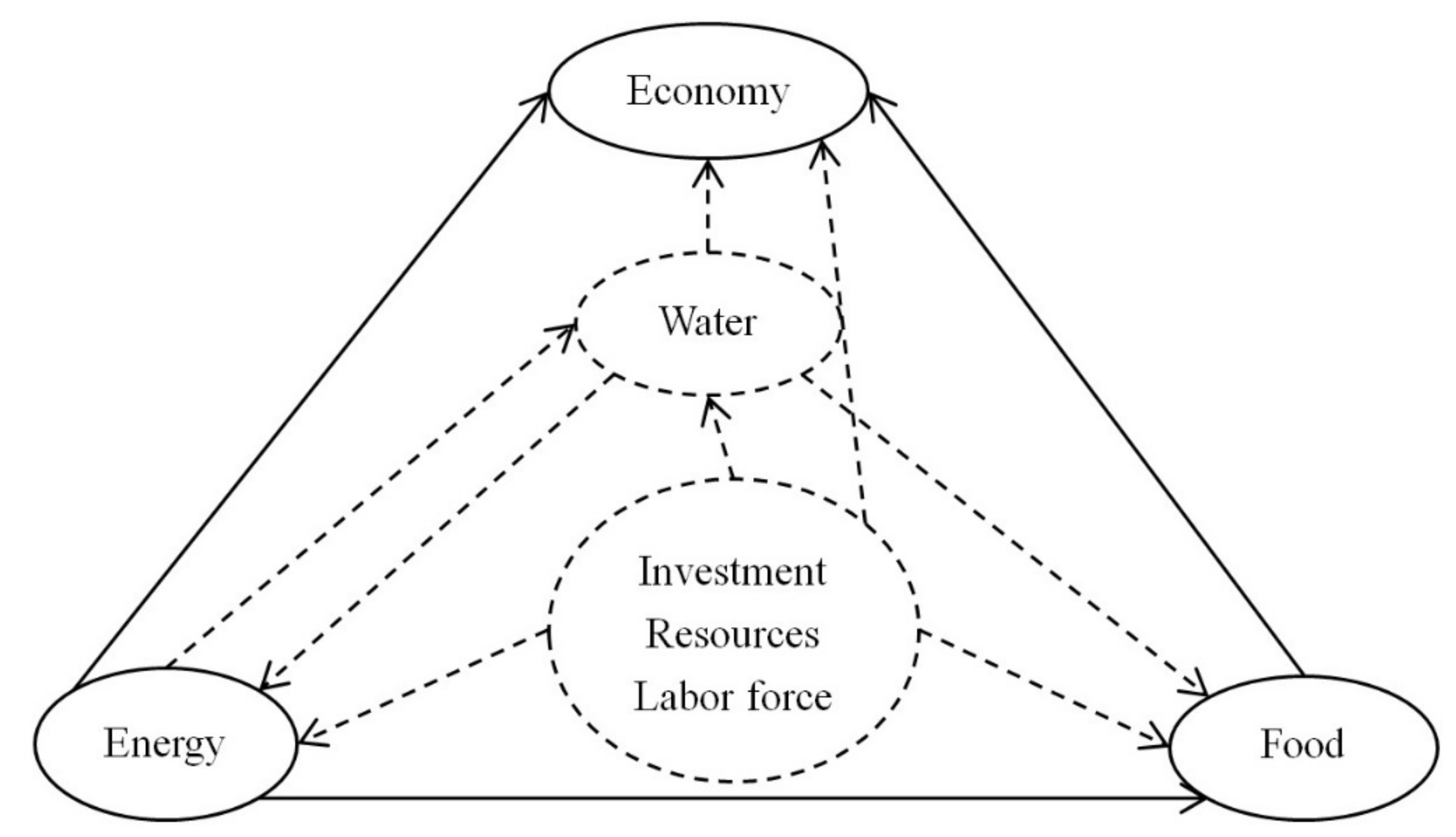
According to the WEF system relationship, we establish the three-dimensional network structure diagram of WEF as shown in Figure 1. We can divide the structure into two stages. The bottom of the pyramid is the first stage. This stage includes the water resources subsystem, the energy subsystem, and the food subsystem. These three subsystems are in a parallel relationship. The arrows in the network structure diagram represent the production process, and the nodes are input or output indicators. Specifically, the water resources subsystem takes water as the output index and energy, investment, resources, and employed population as the input indices. Due to the lack of food input indicators that directly reflect the production needs of the water production industry, the possible food input indicators are the food consumption indicators of water production employees, which belong to indirect input indicators. Therefore, we do not consider the food input indicators in the water system. The energy subsystem takes energy as the output index and relevant water, investment, resources, and employed population as the input index. We do not consider the food input indicators required by the energy production industry because the energy generated by food accounts for a very small proportion of the total energy production, and the relevant indicators are not easy to statistically query. The food subsystem takes food as the output index and relevant water, energy, investment, resources, and employed population as the input indices. In the second stage, from the bottom of the pyramid to the top, economic indicators are taken as the output, and the three outputs of the first stage and related investment, resources, and employed population are taken as the input indicators.
Suppose there are n DMUs, and all indicators and corresponding weights of DMUk (k = 1, 2, …, n) are shown in Table 1.
2.2. DEA Model
We first calculate the efficiency of the three subsystems in the first stage. Different from the traditional definition of efficiency, we define the ratio of input to output as the efficiency value. The notations and their meanings are shown in Table 2.
The efficiency values of these three subsystems are:
Because we use the ratio of input to output to calculate the efficiency value, the calculated efficiency value is greater than or equal to 1. The closer the efficiency value is to 1, the higher the efficiency level of the DMU is.
We use the efficiency aggregation method proposed by Chen et al. [41], and the overall efficiency of the system as the weighted sum of the efficiency values of each subsystem in the first stage is defined as:
We use the proportion of the total output of each system in the total output of all systems to define the weight of each system, and the sum of the weights of the three subsystems is equal to 1:
Taking Formulas (1)–(3), (5)–(7) into Formula (4), the overall efficiency definition formula of the first stage of DMUk (k = 1, 2, …, n) can be changed into the following form:
The efficiency expression of the second stage is:
We still define the overall efficiency of the system as the weighted sum of the efficiency of the two sub stages:
The weight of each stage is defined as the proportion of the total output of each stage in the total output of the system:
Bringing (8), (9), (11), and (12) into (10), the overall efficiency expression of the system is
The overall efficiency of the system can be obtained by calculating the following linear programming:
In order to ensure that the calculated result is the effective value and to make each index play a role, we set the lower bound of the optimal solution to an infinitesimal quantity ε, which can be adjusted according to different examples. The calculation model (14) obtains a set of optimal solutions as
Then, the overall efficiency expression and the efficiency value expression of the three subsystems are respectively:
In view of the situation that multiple solutions will appear in the calculation of this model, we further expand this model with reference to the traditional treatment method of cross-efficiency. For other DMUj (j = 1, 2, …, n), the optimal solution can also be obtained by using linear programming (14). Based on this, the overall cross-efficiency of DMUj using the optimal weight of DMUk in model (14) is defined as:
The above cross-efficiency value determination process is shown in the cross-efficiency matrix E in Table 3. The element Ekj in the matrix is the cross-efficiency value obtained by DMUj (j = 1, 2, …, n) using the weight of DMUk, and the element on the diagonal represents the efficiency value during self-assessment.
For DMUj (j = 1, 2, …, n), the average value of all Ekj (k = 1, 2, …, n), that is, (j = 1, 2, …, n), represents the cross-efficiency value of DMUj. Therefore, the overall cross-efficiency, the cross-efficiency of the two stages, and the cross-efficiency of the three subsystems in the first stage are as follows:
3. Case Analysis
3.1. Establishment of Index System
All data in this paper are from the China Statistical Yearbook, the China Energy Statistical Yearbook, the Statistical Yearbook of Chinese Investment Field, the China Population and Employment Statistics Yearbook, the China Water Resources Bulletin, the National Bureau of Statistics, and provincial statistical yearbooks. For some data not published in the statistical data, we consulted the Statistics Bureau or water resources department of relevant provinces. According to the availability of data, the data of China’s 19 provincial administrative regions (in eastern China, Northeast China, and central China) in 2019 were selected for efficiency calculation. Individual missing values were processed by interpolation method. The specific original data values are shown in Table A2 in the Appendix A.
For the indicators of the water resources subsystem, since the total energy consumption data of water production and supply industry in many provinces cannot be obtained, we use the power consumption of this industry to replace it. In the energy production subsystem, according to the availability of data, we use the relevant indicators of the power and heat production and supply industries to reflect the energy production situation. The water consumption of the power and heat production and supply industries in a few provinces is replaced by the water consumption data of fire (nuclear) power. We choose R&D practitioners as the resources needed for the economic development of each province.
3.2. Efficiency Values and Ranking
We use MATLAB 2018a software to calculate the input–output efficiency of the WEF-Eco systems of 19 provincial administrative regions in 2019. In the calculation process of this example, on the premise of ensuring that the values of expressions (22)–(27) are non-null values, after testing, we determine that the minimum lower bound ε of the solution of model (14) should be 10−4. Before bringing the data into the model calculation, we use the following data standardization methods to process the data:
4. Discussion
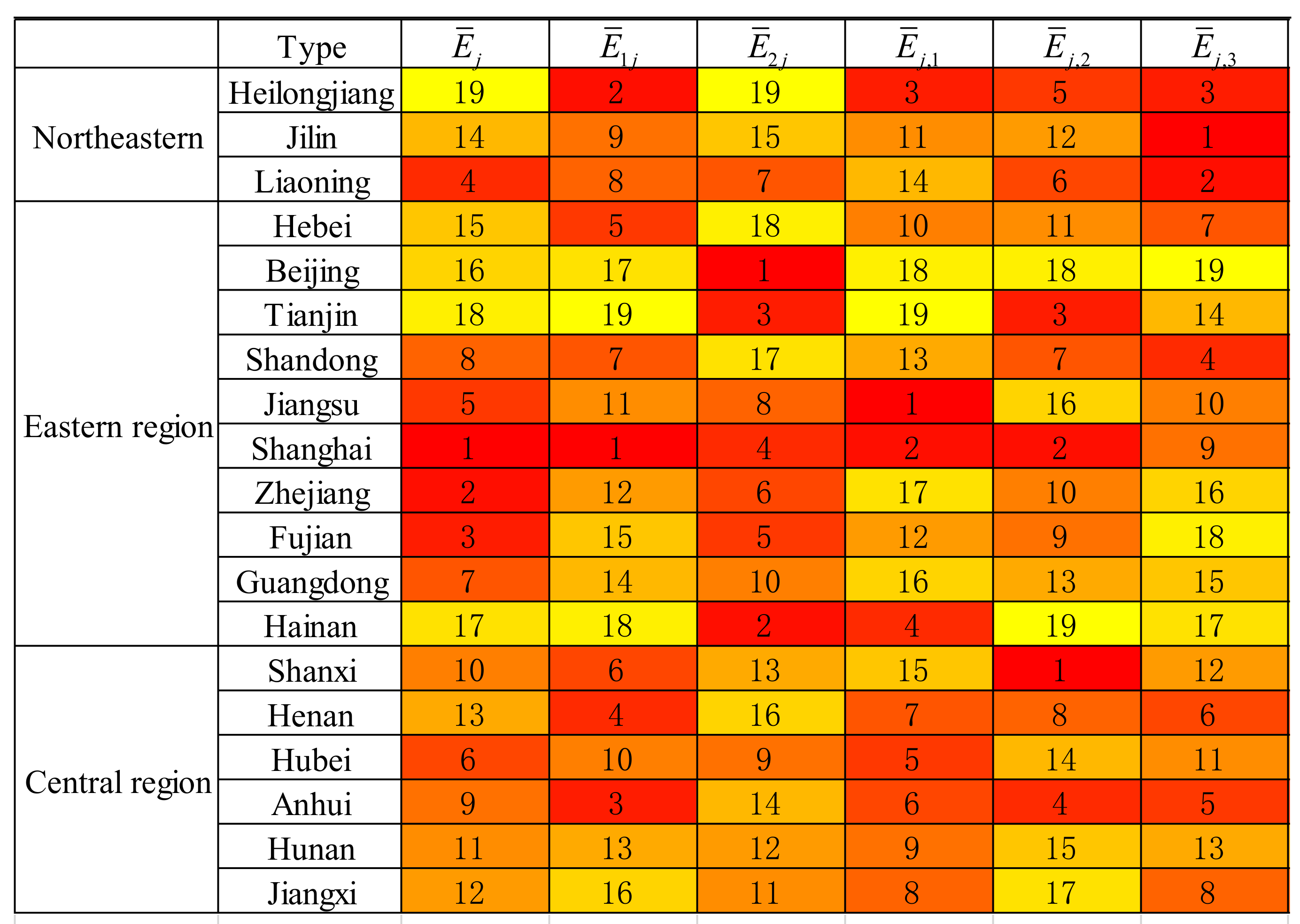
In order to better reflect the regional characteristics of efficiency, we put the provinces belonging to Northeast China, Eastern China, and Central China together. According to the efficiency value ranking, the efficiency value ranking is expressed in a gradual color from yellow to red. The redder the color of the color block, the higher the efficiency level ranking. The yellower the color of the color block, the lower the efficiency level ranking. The results are shown in Figure 2.
From Figure 2, we can intuitively see the regional characteristics and the differences in efficiency in each province. In terms of overall efficiency, the efficiency level of the eastern and central regions is high in the middle and low in the north and south ends. The efficiency level of the northeast region is gradually decreasing from south to north. The provinces with high efficiency levels include Shanghai, Zhejiang, and Fujian. The provinces with low efficiency mainly include Hainan, Tianjin, and Heilongjiang. In terms of the efficiency of the first stage system (WEF system), the regional characteristics are not obvious. The efficiency levels in the three regions are quite different. The efficiency levels of Zhejiang, Heilongjiang, and Anhui are relatively high, while those of Beijing, Hainan, and Tianjin are relatively low. In terms of the system efficiency in the second stage, the regional characteristics are relatively obvious. The provinces with higher efficiency levels are mostly located in the eastern region, while the efficiency levels of other regions are relatively low. Similarly, we can find that the efficiency level of northern provinces is low, while that of southern provinces is high. These characteristics are roughly consistent with the level of economic development in real life. In terms of water resources subsystem, the regional characteristics are not obvious, and the efficiency levels in each region differ greatly. The provinces with high efficiency level mainly include Jiangsu, Shanghai, and Heilongjiang, while the provinces with low efficiency level mainly include Zhejiang, Beijing, and Tianjin. As far as the energy subsystem is concerned, the regional characteristics of efficiency level are not obvious. There are great differences in efficiency level among the three regions. The efficiency value of Shanxi is 1, and the efficiency level is the highest. In addition, the efficiency level of Shanghai and Tianjin is relatively high. The provinces with low efficiency level mainly include Jiangxi, Beijing, and Hainan. As far as the food subsystem is concerned, the efficiency level of Northeast China is the highest, and the efficiency level of central and eastern regions is low. The efficiency value of Beijing is very large, which indicates that the efficiency level is very low, and special attention should be paid to it.
Provinces with higher efficiency levels often have higher management levels, more advanced technology levels, etc., which can make full use of resources for production activities, effectively reduce resource waste, or obtain more output. Through Figure 2, we can clearly find out the reasons for the high and low efficiency levels of systems in different provinces. For example, the overall efficiency level of the system in Shanghai is relatively high. We find that the efficiency level of the first stage (WEF system) and the efficiency level of the second stage in Shanghai are relatively high. The high efficiency level of the first stage is due to the relatively high efficiency of the three subsystems in the WEF system. This kind of province with a high efficiency level in each part tends to develop more comprehensively and is ahead of other provinces in all aspects. However, there may also be situations where the overall efficiency level is high, but some local efficiency levels are low, such as in Zhejiang Province and Fujian Province. The efficiency levels of these two provinces in the first stage are relatively low, but their efficiency levels in the second stage are relatively high, which leads to higher overall efficiency. The main reason for this is that the efficiency level of the second stage has obvious advantages, making up for the impact of the first stage, which has a low efficiency level. The reasons for the efficiency level of other provinces can also be seen from Figure 2. On the contrary, we can also give an improvement method to improve the system efficiency according to the results in Figure 2. For example, the overall efficiency level of Beijing is low. We can find that the efficiency level of the first phase of Beijing is low. To be more precise, the efficiency level of the three subsystems in the first phase is relatively low. We can reduce the waste of resources or increase the output to improve the efficiency level of the three subsystems by introducing advanced management experience and improving the level of science and technology, so as to improve the overall efficiency level of Beijing. Other provinces with low overall efficiency can also accurately find the links to be improved according to the results in Figure 2.
5. Conclusions
This paper establishes a three-dimensional network structure to describe the WEF-Eco system and establishes the corresponding complex network DEA model taking the data of 19 regions in China in 2019 as an example to show the application effect of this model. The innovation of this article is to expand the traditional two-dimensional network used to describe the structure of the WEF system into a three-dimensional network structure which can more accurately describe the structure of the WEF system. We build weights and corresponding models according to the output indicators, and expand the types of DEA models.
In this paper, the structure of the WEF system is shown more clearly, and the calculation method of the overall and local efficiency of the system is proposed, so that we can find the reason for the low efficiency level more accurately and then propose effective improvement methods. In addition, the construction method of the three-dimensional network DEA model proposed in this paper can inspire us to deal with other problems with three-dimensional network structure and even build more complex structures and DEA models. It is also worth noting that in the process of building the additive DEA model, we should not be limited to the traditional weight building method, but should reasonably select input indicators or output indicators to build the weight of each system according to the actual situation, so that the evaluation results are more consistent with the actual situation.
There are still some limitations in this paper. First, in addition to indicators of water resources, energy, and food, we increase the investigation of investment, resources, and labor indicators and do not distinguish the preference relationship between indicators. Second, this paper does not consider the unexpected output, such as the emission of pollutants in the production process. Finally, this paper only considers the efficiency value of a single period, and the dynamic model of multiple periods is not given. All of these are challenges for the future research.
Author Contributions
Z.Z.; writing—original draft preparation; supervision, Y.X. All authors have read and agreed to the published version of the manuscript.
Funding
This research received no external funding.
Institutional Review Board Statement
No Institutional Review Board Statement and approval number.
Informed Consent Statement
Not applicable.
Data Availability Statement
No applicable.
Conflicts of Interest
The authors declare no conflict of interest.
Appendix A

Table A1.
Full names and abbreviations of nouns.
| Full Name | Abbreviation | Full Name | Abbreviation |
|---|---|---|---|
| Water–Energy–Food | WEF | Life Cycle Assessment | LCA |
| Multiregional Input–Output | MRIO | Index System Method | ISM |
| Data Envelopment Analysis | DEA | System Dynamics | SD |
| Coupling Coordination Degree Model | CCDM | Exploratory Spatial Data Analysis | ESDA |
| Geographically Weighted Regression | GWR | Decision Making Unit | DMU |
| Slacks-based Model | SBM | Three-stage, dual-boundary Network DEA | TD-NDEA |
Table A2.
Data of evaluation index system.
| Type | x1k,1 | z1k,1 | z1k,2 | z1k,3 | y1k | x2k,1 | z2k,1 | z2k,2 | y2k | x3k,1 | x3k,2 |
| Beijing | 24.56 | 54.20 | 24.6 | 1.4852 | 41.7 | 0.659 | 153.36 | 6.9453 | 691.1 | 3.7 | 55.75 |
| Tianjin | 8.48 | 107.46 | 8.1 | 0.8051 | 28.4 | 0.5779 | 280.11 | 2.6935 | 5106.83 | 9.2 | 107 |
| Hebei | 23.82 | 208.48 | 113.5 | 3.0811 | 182.3 | 3.7712 | 1578.00 | 13.7431 | 6820 | 114.4 | 50.04 |
| Shanxi | 6.49 | 78.78 | 97.3 | 2.4604 | 76 | 4.14512 | 687.45 | 11.0051 | 69,313.12 | 43.8 | 308.12 |
| Liaoning | 26.02 | 75.26 | 256 | 2.8808 | 130.3 | 0.1 | 439.46 | 11.1454 | 4441.1 | 80.7 | 302.12 |
| Jilin | 17.71 | 120.44 | 506.1 | 1.7157 | 115.4 | 5.39 | 171.99 | 8.0834 | 2288.2 | 81.5 | 149.68 |
| Heilongjiang | 9.57 | 216.83 | 1511.4 | 2.2036 | 310.4 | 7.1 | 380.53 | 11.6212 | 9766.93 | 274.2 | 658.9 |
| Shanghai | 6.47 | 116.62 | 48.3 | 0.964 | 100.9 | 49.87 | 123.21 | 1.8695 | 42,674.352 | 16.9 | 59.57 |
| Jiangsu | 41.36 | 266.59 | 231.7 | 4.122 | 619.1 | 80.5 | 869.88 | 8.4166 | 3489.29 | 619.1 | 550.24 |
| Zhejiang | 30.56 | 182.23 | 1321.5 | 3.3197 | 165.8 | 0.7 | 625.19 | 6.7434 | 2937 | 72.4 | 421 |
| Anhui | 19.32 | 434.87 | 539.9 | 1.985 | 277.7 | 4.77541 | 555.78 | 7.419 | 8943.62 | 150.2 | 259.48 |
| Fujian | 8.86 | 466.95 | 1363.9 | 1.7629 | 177.5 | 1.04436 | 634.48 | 9.1325 | 4353.87 | 83.7 | 252.57 |
| Jiangxi | 12.21 | 155.24 | 2051.6 | 2.0534 | 253.3 | 18.09 | 408.14 | 6.7125 | 1320.3 | 162.5 | 152.44 |
| Shandong | 40.97 | 350.79 | 195.2 | 3.6952 | 225.3 | 7.410074 | 1568.71 | 22.1594 | 12,539.1 | 138.2 | 599.7 |
| Henan | 11.1 | 299.89 | 168.6 | 3.7418 | 237.8 | 4.1549 | 1574.82 | 17.7199 | 10,303.95 | 121.8 | 572 |
| Hubei | 10.11 | 437.47 | 613.7 | 2.5862 | 303.2 | 45 | 678.72 | 11.1438 | 4892.2 | 155.6 | 452 |
| Hunan | 14.27 | 602.98 | 2098.3 | 2.9797 | 333 | 38.9 | 693.39 | 11.5254 | 3000 | 191.7 | 523.88 |
| Guangdong | 72.07 | 831.13 | 2068.2 | 6.4027 | 412.3 | 35.7 | 1338.49 | 17.437 | 8377.25 | 208.5 | 618.21 |
| Hainan | 3.61 | 50.56 | 252.3 | 0.6518 | 46.4 | 38.66 | 161.98 | 1.3652 | 494.08 | 34.2 | 109.66 |
| Type | z3k,1 | z3k,2 | z3k,3 | y3k | x4k,1 | x4k,2 | x4k,3 | z4k,1 | z4k,2 | z4k,3 | y4k |
| Beijing | 125.95 | 46.52 | 42.4 | 28.76 | 41.7 | 691.1 | 28.76 | 7868.74 | 6.5486 | 1273 | 164,563 |
| Tianjin | 270.06 | 339.27 | 58.28 | 223.25 | 28.4 | 5106.83 | 223.25 | 12,112.08 | 6.6307 | 896.56 | 90,058 |
| Hebei | 1595.11 | 6469.17 | 1331.15 | 3739.24 | 182.3 | 6820 | 3739.24 | 717,100.30 | 11.6854 | 4182.46 | 46,182 |
| Shanxi | 285.50 | 3126.17 | 666.7 | 1361.8 | 76 | 69,313.12 | 1361.8 | 7094.59 | 4.474 | 1902.5 | 45,549 |
| Liaoning | 121.98 | 3488.73 | 510 | 2429.95 | 130.3 | 4441.1 | 2429.95 | 6716.57 | 7.8128 | 2238.4 | 57,067 |
| Jilin | 442.85 | 5644.93 | 466.2 | 3877.93 | 115.4 | 2288.2 | 3877.93 | 11,285.40 | 2.0809 | 1456.43 | 43,475 |
| Heilongjiang | 990.52 | 14,338.1 | 564.1 | 7503.01 | 310.4 | 9766.93 | 7503.01 | 8837.84 | 2.3123 | 1776.9 | 36,001 |
| Shanghai | 3.51 | 117.37 | 40.8 | 95.89 | 100.9 | 42,674.352 | 95.89 | 8012.22 | 11.3425 | 1376.2 | 156,587 |
| Jiangsu | 383.94 | 5381.48 | 734.51 | 3706.2 | 619.1 | 3489.29 | 3706.2 | 58,766.89 | 69.3442 | 4745.2 | 122,398 |
| Zhejiang | 99.38 | 977.44 | 406.83 | 592.15 | 165.8 | 2937 | 592.15 | 36,702.88 | 57.4571 | 3875.1 | 107,814 |
| Anhui | 761.48 | 7287 | 1346.9 | 4054 | 277.7 | 8943.62 | 4054 | 35,631.90 | 18.358 | 4384 | 58,072 |
| Fujian | 1327.45 | 822.43 | 548.85 | 493.9 | 177.5 | 4353.87 | 493.9 | 31,164.02 | 18.0365 | 2781.26 | 106,966 |
| Jiangxi | 471.50 | 3665.14 | 700.8 | 2157.45 | 253.3 | 1320.3 | 2157.45 | 26,794.15 | 12.2207 | 2631.95 | 52,865 |
| Shandong | 996.96 | 8312.81 | 1445.9 | 5357 | 225.3 | 12539.1 | 5357 | 591,438.30 | 30.4172 | 5987.9 | 70,129 |
| Henan | 2460.42 | 10,734.54 | 2277 | 6695.36 | 237.8 | 10,303.95 | 6695.36 | 51,241.12 | 20.6775 | 6562 | 55,825 |
| Hubei | 1052.38 | 4608.6 | 1164 | 2724.98 | 303.2 | 4892.2 | 2724.98 | 39,128.68 | 17.5724 | 3548 | 76,712 |
| Hunan | 2114.48 | 4616.38 | 1409.24 | 2974.84 | 333 | 3000 | 2974.84 | 37,941.46 | 16.088 | 3666.48 | 57,746 |
| Guangdong | 321.51 | 2160.64 | 823 | 1240.8 | 412.3 | 8377.25 | 1240.8 | 46,093.28 | 83.8891 | 7150.25 | 94,448 |
| Hainan | 36.84 | 272.65 | 175.15 | 144.96 | 46.4 | 494.08 | 144.96 | 3277.63 | 0.2832 | 102.2 | 56,740 |
References
- Jiao, Y.J. Spatial and temporal evolution characteristics of the coupling and coordination among water, energy and food in Anhui province. Hubei Agric. Sci. 2021, 60, 184–191. [Google Scholar]
- Rasul, G.; Sharma, B. The nexus approach to water-energy-food security: An option for adaptation to climate change. Clim. Policy 2015, 16, 682–702. [Google Scholar] [CrossRef] [Green Version]
- Conway, D.; Garderen, E.A.V.; Deryng, D.; Dorling, S.; Krueger, T.; Landman, W.; Lankford, B.; Lebek, K.; Osborn, T.; Ringler, C.; et al. Climate and southern Africa’s water-energy-food nexus. Nat. Clim. Chang. 2015, 5, 837–846. [Google Scholar] [CrossRef] [Green Version]
- Li, G.J.; Huang, D.H.; Li, Y.L. Water-energy-food nexus (WEF-Nexus): New perspective on regional sustainable development. J. Cent. Univ. Financ. Econ. 2016, 36, 76–90. [Google Scholar]
- Hussien, W.E.A.; Memon, F.A.; Savic, D.A. A risk-based assessment of the household water-energy-food nexus under the impact of seasonal variability. J. Clean. Prod. 2018, 171, 1275–1289. [Google Scholar] [CrossRef]
- Zhang, X.D.; Vesselinov, V.V. Integrated modeling approach for optimal management of water, energy and food security nexus. Adv. Water Resour. 2017, 101, 1–10. [Google Scholar] [CrossRef]
- Howarth, C.; Monasterolo, I. Understanding barriers to decision making in the UK energy-food-water nexus: The added value of interdisciplinary approaches. Environ. Sci. Policy 2016, 61, 53–60. [Google Scholar] [CrossRef] [Green Version]
- Zhang, C.; Chen, X.X.; Li, Y.; Ding, W.; Fu, G.T. Water-energy-food nexus: Concepts, questions and methodologies. J. Clean. Prod. 2018, 195, 625–639. [Google Scholar] [CrossRef]
- Chen, J.F.; Ding, T.H.; Li, M.; Wang, H.M. Multi-Objective Optimization of a Regional Water-Energy-Food System Considering Environmental Constraints: A Case Study of Inner Mongolia, China. Int. J. Environ. Res. Public Health 2020, 17, 6834. [Google Scholar] [CrossRef]
- Purwanto, A.; Sušnik, J.; Suryadi, F.X.; Fraiture, C.D. Using group model building to develop a causal loop mapping of the water-energy-food security nexus in Karawang Regency, Indonesia. J. Clean. Prod. 2019, 240, 118170. [Google Scholar] [CrossRef]
- Chen, I.C.; Wang, Y.H.; Lin, W.; Ma, H.W. Assessing the risk of the food-energy-water nexus of urban metabolism: A case study of Kinmen Island, Taiwan. Ecol. Indic. 2020, 110, 105861. [Google Scholar] [CrossRef]
- Ji, L.; Zhang, B.B.; Huang, G.; Lu, Y. Multi-stage stochastic fuzzy random programming for food-water-energy nexus management under uncertainties. Resour. Conserv. Recycl. 2020, 155, 104665. [Google Scholar] [CrossRef]
- Sherwood, J.; Clabeaux, R.; Carbajales-Dale, M. An extended environmental input-output lifecycle assessment model to study the urban food-energy-water nexus. Environ. Res. Lett. 2017, 12, 105003. [Google Scholar] [CrossRef]
- Li, X.; Feng, K.S.; Siu, Y.L.; Hubacek, K. Energy-water nexus of wind power in China: The balancing act between CO2 emissions and water consumption. Energy Policy 2012, 45, 440–448. [Google Scholar] [CrossRef]
- Salmoral, G.; Yan, X.Y. Food-energy-water nexus: A life cycle analysis on virtual water and embodied energy in food consumption in the Tamar catchment, UK. Resour. Conserv. Recycl. 2018, 133, 320–330. [Google Scholar] [CrossRef]
- White, D.J.; Hubacek, K.; Feng, K.S.; Sun, L.X.; Meng, B. The Water-Energy-Food Nexus in East Asia: A tele-connected value chain analysis using inter-regional input-output analysis. Appl. Energy 2018, 210, 550–567. [Google Scholar] [CrossRef] [Green Version]
- Chen, W.M.; Wu, S.M.; Lei, Y.L.; Li, S.T. China’s water footprint by province, and inter-provincial transfer of virtual water. Ecol. Indic. 2017, 74, 321–333. [Google Scholar] [CrossRef]
- Zhang, B.; Qu, X.; Meng, J.; Sun, X.D. Identifying primary energy requirements in structural path analysis: A case study of China 2012. Appl. Energy 2017, 191, 425–435. [Google Scholar] [CrossRef] [Green Version]
- Schlör, H.; Venghaus, S.; Hake, J.F. The FEW-Nexus city index—Measuring urban resilience. Appl. Energy 2018, 210, 382–392. [Google Scholar] [CrossRef]
- Ozturk, I. Sustainability in the food-energy-water nexus: Evidence from BRICS (Brazil, the Russian Federation, India, China, and South Africa) countries. Energy 2015, 93, 999–1010. [Google Scholar] [CrossRef]
- Li, G.J.; Huang, D.H.; Li, Y.L. Evaluation on the Efficiency of the Input and Output of Water-Energy-Food in Different Regions of China. Comp. Econ. Soc. Syst. 2017, 3, 138–148. [Google Scholar]
- Chen, Z.X.; Zhang, S.Q.; Li, C.Y. Research on Inter-provincial Water-Energy-Food Comprehensive Utilization Efficiency in China. J. Shandong Univ. Sci. Technol. Soc. Sci. 2021, 23, 84–93. [Google Scholar]
- Halbe, J.; Wostl, C.P.; Lange, M.A.; Velonis, C. Governance of transitions towards sustainable development—The water-energy-food nexus in Cyprus. Water Int. 2015, 40, 877–894. [Google Scholar] [CrossRef]
- Wang, H.M.; Hong, J.; Liu, G. Simulation research on different policies of regional green development under the nexus of water-energy-food. Chin. J. Popul. Resour. Environ. 2019, 29, 74–84. [Google Scholar]
- Liu, L.Y.; Wang, H.M.; Liu, G.; Sun, D.Y.; Fang, Z. Driving mechanism and policy simulation of Water-Energy-Food risks from the perspective of supply and demand—A case study of Northeast China for system dynamics analysis. Soft Sci. 2020, 34, 52–60. [Google Scholar]
- Mi, H.; Zhou, W. The system simulation of China’s grain, fresh water and energy demand in the next 30 years. Popul. Econ. 2010, 31, 1–7. [Google Scholar]
- Li, G.J.; Li, Y.L.; Jia, X.J.; Du, L.; Huang, D.H. Establishment and Simulation Study of System Dynamic Model on Sustainable Development of Water-Energy-Food Nexus in Beijing. Manag. Rev. 2016, 28, 11–26. [Google Scholar]
- Peng, S.M.; Zheng, X.K.; Wang, Y.; Jiang, G.Q. Study on water-energy-food collaborative optimization for Yellow River basin. Adv. Water Resour. 2017, 28, 681–690. [Google Scholar]
- Deng, P.; Chen, J.; Chen, D.; Shi, H.Y.; Bi, B.; Liu, Z.; Yin, Y.; Cao, X.C. The evolutionary characteristics analysis of the coupling and coordination among water, energy and food: Take Jiangsu Province as an example. J. Water Resour. Water Eng. 2017, 28, 232–238. [Google Scholar]
- Bi, B.; Chen, D.; Deng, P.; Zhang, D.; Zhu, L.Y.; Zhang, P. The evolutionary characteristics analysis of coupling and coordination of regional Water-Energy-Food. Chin. Rural Water Hydropower 2018, 60, 72–77. [Google Scholar]
- Li, C.Y.; Zhang, S.Q. Chinese provincial water-energy-food coupling coordination degree and influencing factors research. Chin. J. Popul. Resour. Environ. 2020, 30, 120–128. [Google Scholar]
- Sun, C.Z.; Yan, X.D. Security evaluation and spatial correlation pattern analysis of water resources-energy-food nexus coupling system in China. Water Resour. Prot. 2018, 34, 1–8. [Google Scholar]
- Bai, J.F.; Zhang, H.J. Spatio-temporal Variation and Driving Force ofWater-Energy-Food Pressure in China. Sci. Geogr. Sin. 2018, 38, 1653–1660. [Google Scholar]
- Charnes, A.; Cooper, W.W.; Rhodes, E. Measuring the efficiency of decision making units. Eur. J. Oper. Res. 1978, 2, 429–444. [Google Scholar] [CrossRef]
- Banker, R.D.; Charnes, A.; Cooper, W.W. Some models for estimating technical and scale inefficiencies in DEA. Manag. Sci. 1984, 32, 1613–1627. [Google Scholar] [CrossRef]
- Liang, L.; Wu, J. A retrospective and perspective view on cross efficiency of data envelopment analysis (DEA). J. Univ. Sci. Technol. China 2013, 43, 941–947. [Google Scholar]
- Kao, C.; Liu, S.T. Cross efficiency measurement and decomposition in two basic network systems. Omega 2018, 83, 70–79. [Google Scholar] [CrossRef]
- Färe, R.; Grosskopf, S. Network DEA. Socio-Econ. Plan. Sci. 2000, 3, 35–49. [Google Scholar] [CrossRef]
- Kao, C.; Hwang, S.N. Efficiency decomposition in two-stage data envelopment analysis: An application to non-life insurance companies in Taiwan. Eur. J. Oper. Res. 2008, 185, 418–429. [Google Scholar] [CrossRef]
- Tone, K.; Tsutsui, M. Network DEA: A slacks-based measure approach. Eur. J. Oper. Res. 2009, 197, 243–252. [Google Scholar] [CrossRef] [Green Version]
- Chen, Y.; Cook, W.D.; Li, N.; Zhu, J. Additive efficiency decomposition in two-stage DEA. Eur. J. Oper. Res. 2009, 196, 1170–1176. [Google Scholar] [CrossRef]
- Sexton, T.R.; Silkman, R.H.; Hogan, A.J. Data envelopment analysis: Critique and extensions. New Dir. Program Eval. 1986, 1986, 73–105. [Google Scholar] [CrossRef]
- Doyle, J.; Green, R. Efficiency and Cross-efficiency in DEA: Derivations, Meanings and Uses. J. Oper. Res. Soc. 1994, 45, 567–578. [Google Scholar] [CrossRef]
- Wang, Y.M.; Chin, K.S. A neutral DEA model for cross-efficiency evaluation and its extension. Expert Syst. Appl. 2010, 37, 3666–3675. [Google Scholar] [CrossRef]
- Wang, Y.M.; Chin, K.S.; Jiang, P. Weight determination in the cross-efficiency evaluation. Comput. Ind. Eng. 2011, 61, 497–502. [Google Scholar] [CrossRef]
- Li, C.H.; Su, H.; Tong, Y.J.; Sun, Y.H. DEA Cross-Efficiency Evaluation Model by the Solution Strategy Referring to the Ideal DMU. Chin. J. Manag. Sci. 2015, 23, 116–122. [Google Scholar] [CrossRef]
- Liu, W.L.; Wang, Y.M.; Lv, S.L. Ranking Decision Making Units Based on Cross-efficiency and Cooperative Game. Chin. J. Manag. Sci. 2018, 26, 163–170. [Google Scholar]
- Sun, C.Z.; Hao, S.; Zhao, L.S. Spatial-temporal differentiation characteristics of water resources-energy-food nexus system efficiency in China. Water Resour. Prot. 2021, 37, 61–68+78. [Google Scholar]
- Li, J.X.; Wang, L.H.; Wei, G.; Gong, Z.W.; Zhao, Y.Z.; Liu, S.J. Water-Energy-Food Nexus and Eco-Sustainability: A Three-Stage Dual-Boundary Network DEA Model for Evaluating Jiangsu Province in China. Int. J. Comput. Intell. Syst. 2021, 14, 1501. [Google Scholar] [CrossRef]
Figure 1.
Three-dimensional network structure of the WEF-Eco system.

Figure 2.
Ranking chart of different efficiency values in different province. (the efficiency value ranking is expressed in a gradual color from yellow to red. The redder the color of the color block, the higher the efficiency level ranking. The yellower the color of the color block, the lower the efficiency level ranking.).

Table 1.
The notations and their meaning.
| Notations | Definitions |
|---|---|
| E1k,i | Efficiency value of ith subsystem in the first stage of the DMUk (i = 1, 2, 3) |
| Ejk | Efficiency of the jth stage of the DMUk (j = 1, 2) |
| Ekk | Overall efficiency of the DMUk (self-assessment) |
| ω1k,i | Weight of ith subsystem in the first stage of the DMUk (i = 1, 2, 3) |
| ωjk | Weight of the jth stage of the DMUk (j = 1, 2) |
| τik,1 | Weight of investment index of the ith subsystem of the first stage of the DMUk (i = 1, 2, 3) |
| τik,2 | Weight of resources index of the ith subsystem of the first stage of the DMUk (i = 1, 2, 3) |
| τik,3 | Weight of labor force index of the ith subsystem of the first stage of the DMUk (i = 1, 2, 3) |
| v1k,1 | Weight of energy input index in the water resources subsystem of the first stage of the DMUk |
| v2k,1 | Weight of water resources input index in the energy subsystem of the first stage of the DMUk |
| v3k,1 | Weight of water resources input index in the food subsystem of the first stage of the DMUk |
| v3k,2 | Weight of energy input index in the food subsystem of the first stage of the DMUk |
| uik | Weight of output index of the ith subsystem of the first stage of the DMUk (i = 1, 2, 3) |
Table 2.
Efficiency evaluation index system of the WEF-Eco system.
| Stage | Category | Index | Unit | Notation | Weight |
|---|---|---|---|---|---|
| W-E-F | Water supply subsystem | Total electric power consumption of water production and supply industry | 100 million kWh | x1k,1 | v1k,1 |
| Investment in water production and supply | 100 million yuan | z1k,1 | τ1k,1 | ||
| Total regional water resources | 100 million cu.m | z1k,2 | τ1k,2 | ||
| Employment in water production and supply | 10,000 persons | z1k,3 | τ1k,3 | ||
| Total water supply | 100 million cu.m | y1k | u1k | ||
| Energy production subsystem | Water consumption of electric power and heat power production and supply industry | 100 million cu.m | x2k,1 | v2k,1 | |
| Investment in the production and supply of electric power and heat power | 100 million yuan | z2k,1 | τ2k,1 | ||
| Employment in the production and supply of electric power and heat power | 10,000 persons | z2k,2 | τ2k,2 | ||
| Total energy production | 10,000 tons of SCE | y2k | u2k | ||
| Food production subsystem | Total agricultural water consumption | 100 million cu.m | x3k,1 | v3k,1 | |
| Total Energy consumption of agriculture, forestry, animal production and hunting | 10,000 tons of SCE | x3k,2 | v3k,2 | ||
| Investment in primary industry | 100 million yuan | z3k,1 | τ3k,1 | ||
| Grain sowing area | 1000 hectares | z3k,2 | τ3k,2 | ||
| Number of employees in the primary industry | 10,000 persons | z3k,3 | τ3k,3 | ||
| Total grain production | 10,000 tons | y3k | u3k | ||
| WEF-Eco | Economic development subsystem | Total water supply | 100 million cu.m | x4k,1 | v4k,1 |
| Total energy production | 10,000 tons of SCE | x4k,2 | v4k,2 | ||
| Total grain production | 10,000 tons | x4k,3 | v4k,3 | ||
| Total investment in fixed assets | 100 million yuan | z4k,1 | τ4k,1 | ||
| R&D number of Industrial Enterprises above Designated Size | 10,000 persons | z4k,2 | τ4k,2 | ||
| Number of employed population at the end of the year | 10,000 persons | z4k,3 | τ4k,3 | ||
| Per capita GDP | 100 million yuan | y4k | u4k |
Table 3.
Cross efficiency matrix (CEM).
| DMUk | DMUj | ||||
|---|---|---|---|---|---|
| 1 | 2 | 3 | ⋯ | n | |
| 1 | E11 | E12 | E13 | ⋯ | E1n |
| 2 | E21 | E22 | E23 | E2n | |
| 3 | E31 | E32 | E33 | ⋯ | E3n |
| ⋯ | ⋯ | ⋯ | ⋯ | ⋯ | ⋯ |
| ⋯ | ⋯ | ⋯ | ⋯ | ⋯ | ⋯ |
| ⋯ | ⋯ | ⋯ | ⋯ | ⋯ | ⋯ |
| n | En1 | En2 | En3 | ⋯ | Enn |
| Average value | ⋯ | ||||
Table 4.
WEF-Eco system efficiency values.
| Type | Ranking | Ranking | Ranking | |||
|---|---|---|---|---|---|---|
| Beijing | 24.06 | 16 | 211.45 | 17 | 1.00 | 1 |
| Tianjin | 1264.69 | 18 | 3187.09 | 19 | 2.36 | 3 |
| Hebei | 21.09 | 15 | 2.67 | 5 | 220.11 | 18 |
| Shanxi | 13.90 | 10 | 2.67 | 6 | 42.81 | 13 |
| Liaoning | 8.19 | 4 | 2.71 | 8 | 20.76 | 7 |
| Jilin | 19.92 | 14 | 3.01 | 9 | 57.63 | 15 |
| Heilongjiang | 9897.34 | 19 | 1.81 | 2 | 707,919,722.99 | 19 |
| Shanghai | 2.10 | 1 | 1.72 | 1 | 2.82 | 4 |
| Jiangsu | 8.27 | 5 | 3.70 | 11 | 21.15 | 8 |
| Zhejiang | 5.12 | 2 | 4.08 | 12 | 12.68 | 6 |
| Anhui | 12.99 | 9 | 2.08 | 3 | 43.70 | 14 |
| Fujian | 5.17 | 3 | 4.51 | 15 | 7.58 | 5 |
| Jiangxi | 15.22 | 12 | 4.96 | 16 | 39.08 | 11 |
| Shandong | 10.14 | 8 | 2.68 | 7 | 69.21 | 17 |
| Henan | 17.29 | 13 | 2.41 | 4 | 61.81 | 16 |
| Hubei | 8.32 | 6 | 3.19 | 10 | 21.40 | 9 |
| Hunan | 15.07 | 11 | 4.36 | 13 | 41.78 | 12 |
| Guangdong | 8.73 | 7 | 4.38 | 14 | 28.02 | 10 |
| Hainan | 931.98 | 17 | 2676.13 | 18 | 1.38 | 2 |
Table 5.
Efficiency values of three subsystems in the first stage.
| Type | Ranking | Ranking | Ranking | |||
|---|---|---|---|---|---|---|
| Beijing | 17.12 | 18 | 111.73 | 18 | 1,766,195.52 | 19 |
| Tianjin | 13,677,286.78 | 19 | 2.83 | 3 | 2.95 | 14 |
| Hebei | 2.81 | 10 | 18.89 | 11 | 1.84 | 7 |
| Shanxi | 3.76 | 15 | 1.00 | 1 | 2.51 | 12 |
| Liaoning | 3.73 | 14 | 12.38 | 6 | 1.39 | 2 |
| Jilin | 3.32 | 11 | 20.67 | 12 | 1.09 | 1 |
| Heilongjiang | 1.57 | 3 | 6.78 | 5 | 1.48 | 3 |
| Shanghai | 1.20 | 2 | 2.60 | 2 | 1.96 | 9 |
| Jiangsu | 1.17 | 1 | 78.02 | 16 | 2.30 | 10 |
| Zhejiang | 4.68 | 17 | 17.86 | 10 | 4.05 | 16 |
| Anhui | 2.01 | 6 | 6.10 | 4 | 1.77 | 5 |
| Fujian | 3.53 | 12 | 13.76 | 9 | 6.98 | 18 |
| Jiangxi | 2.17 | 8 | 85.85 | 17 | 1.95 | 8 |
| Shandong | 3.56 | 13 | 12.96 | 7 | 1.62 | 4 |
| Henan | 2.09 | 7 | 13.66 | 8 | 1.82 | 6 |
| Hubei | 1.75 | 5 | 35.77 | 14 | 2.38 | 11 |
| Hunan | 2.71 | 9 | 58.31 | 15 | 2.76 | 13 |
| Guangdong | 4.29 | 16 | 24.12 | 13 | 4.00 | 15 |
| Hainan | 1.74 | 4 | 123,927,931.15 | 19 | 5.47 | 17 |
Publisher’s Note: MDPI stays neutral with regard to jurisdictional claims in published maps and institutional affiliations. |
© 2022 by the authors. Licensee MDPI, Basel, Switzerland. This article is an open access article distributed under the terms and conditions of the Creative Commons Attribution (CC BY) license (https://creativecommons.org/licenses/by/4.0/).
Share and Cite
MDPI and ACS Style
Zhang, Z.; Xu, Y. Evaluation of Water—Energy—Food—Economy Coupling Efficiency Based on Three-Dimensional Network Data Envelopment Analysis Model. Water 2022, 14, 3133. https://doi.org/10.3390/w14193133
AMA Style
Zhang Z, Xu Y. Evaluation of Water—Energy—Food—Economy Coupling Efficiency Based on Three-Dimensional Network Data Envelopment Analysis Model. Water. 2022; 14(19):3133. https://doi.org/10.3390/w14193133
Chicago/Turabian StyleZhang, Zhiyu, and Yejun Xu. 2022. "Evaluation of Water—Energy—Food—Economy Coupling Efficiency Based on Three-Dimensional Network Data Envelopment Analysis Model" Water 14, no. 19: 3133. https://doi.org/10.3390/w14193133
Note that from the first issue of 2016, this journal uses article numbers instead of page numbers. See further details here.