The Impact of Floating Raft Aquaculture on the Hydrodynamic Environment of an Open Sea Area in Liaoning Province, China

Abstract

The sea area of Changhai County in Dalian City is a typical floating raft aquaculture area, located in Liaoning Province, China, where a key issue in determining the scale and spatial layout of the floating raft aquaculture is the assessment of the impact of aquaculture activities on the hydrodynamic environment. To address this issue, we established depth-averaged two-dimensional shallow water equations and three-dimensional incompressible Reynolds-averaged Navier–Stokes equations for the open sea area described in this paper. The impact of floating rafts for aquaculture on hydrodynamic force was reflected in the numerical model by changing the Manning number, where scenarios with different aquaculture densities were taken into account. Finally, the water exchange rate of the floating raft aquaculture area in the study area was calculated. It was found, through a comparison between the simulated value and the measured value obtained via layered observation, that the two values were in good agreement with each other, indicating that the model exhibits great accuracy. In addition, the calculation results for scenarios before and after aquaculture were compared and analyzed, showing that from low-density to high-density aquaculture zones, the variation in flow rate was greater than 80% at the peak of a flood tide. The water exchange rates of the water body after 1 day, 4 days, and 8 days of water exchange were also calculated, and the results show that they had been reduced by 17.92%, 13.59%, and 1.63%, respectively, indicating that the existence of floating rafts for aquaculture indeed reduced the water exchange capacity of the water body. The model described in this paper can serve as a foundation for other studies on aquaculture in open sea areas, and it provides a theoretical basis for the scientific formulation of marine aquaculture plans and the rational optimization of the spatial layout.

1. Introduction

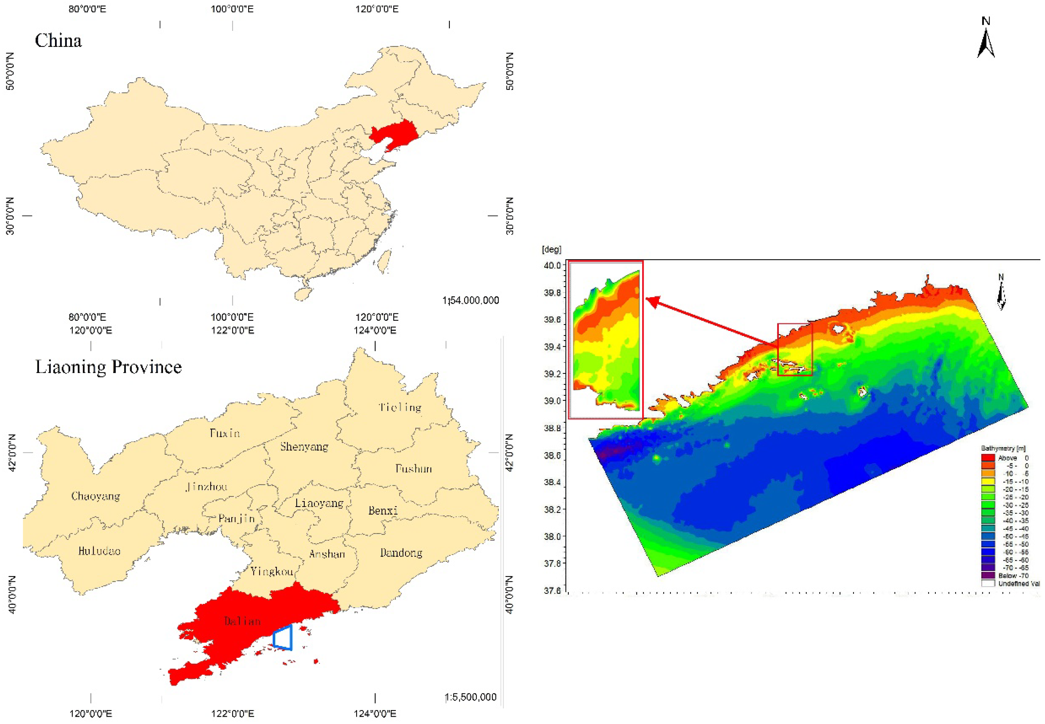
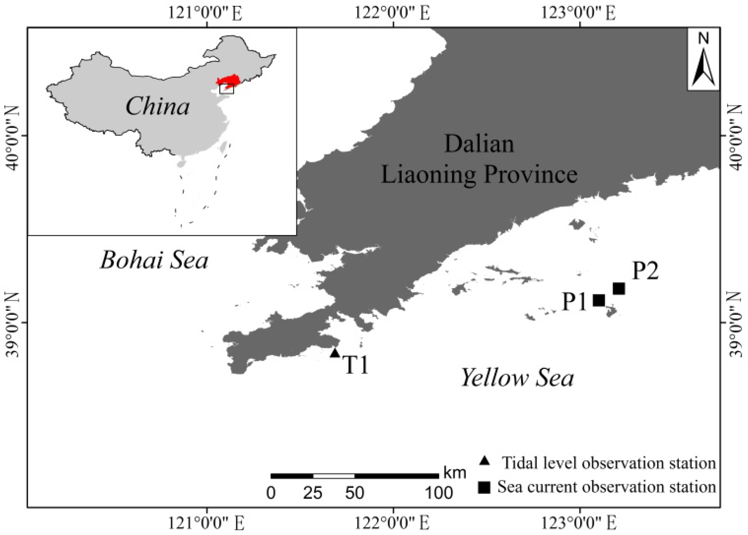
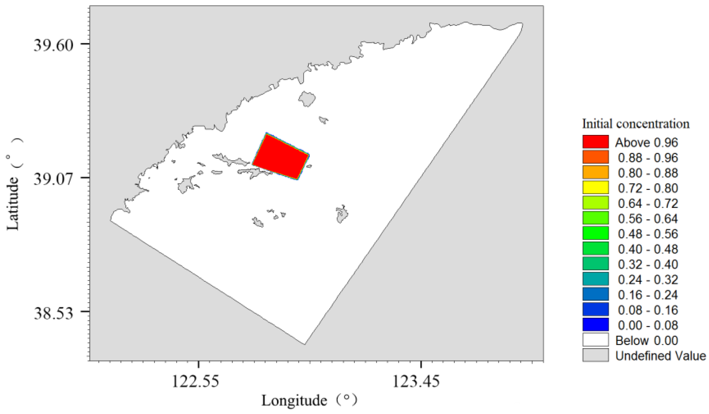
Changhai County, Dalian, is located on the eastern side of the Liaodong Peninsula in the northern waters of the Yellow Sea in Liaoning Province, China(as shown in Figure 1), and its geographic coordinates are 122°17′E–123°13′E, 38°55′N–39°35′N. As the only county completely located on islands in Northeast China, Changhai County has an area of water covering 10,324 square kilometers, which is an ideal habitat for temperate marine organisms, such as fish, shrimp, shellfish, and algae. In recent years, with the rapid development of the marine aquaculture industry, floating raft and cage aquaculture industries have emerged in this open sea area, which has brought not only a great deal of economic benefits to residents, but also huge challenges to marine hydrodynamics and ecological environment protection. Some aquaculture farmers excessively pursue high yields with a lack of scientific and reasonable justification, so they tend to increase the scale and density of aquaculture in a disorderly manner. Due to the over-crowded raft areas, the rafts and facilities have had a hindering effect on the hydrodynamic environment, inhibiting water exchange and weakening the substance transport and diffusion capacity of the water body. As a result, it is impossible for algae and bait to be evenly distributed with the hydrodynamic force, which would support the growth of marine organisms. This results in a phenomenon where the cultured organisms that were longitudinally arranged in a raft area appear to grow well, while those in the middle grow slowly or even die due to a lack of bait. Some aquaculture operators who have been cultivating scallops, oysters, or sea cucumbers in floating rafts and cages have gradually realized the severity of the problem. Thanks to such changes in their awareness, they are looking for a scientific and reasonable solution to the problem, with the ultimate goal of determining the degree of impact of the overall structure for aquaculture, including rafts, floaters, ropes and cages, and even the cultured organisms, on the hydrodynamic environment of an open sea area. The solution of this problem could provide technical support for the scientific formulation of a sowing density plan for cultured organisms, the rational selection of the location of an aquaculture area, and the precise placement of bait casting devices in bait-deficient zones.

In recent years, some researchers have carried out relevant studies on the mechanisms of interactions between raft placement and hydrodynamic environments in raft aquaculture areas; however, most of the studies have focused on the changes in water quality and the sediment environment or used field observations and model tests. For example, Zhao et al. [1] conducted a simulation-based assessment of the impact of the deep-sea cage aquaculture of Lateolabraxjaponicus on water quality and the sediment environment in the Yellow Sea of China based on a three-dimensional Lagrangian particle tracking model. Water quality simulations indicated that deep sea cages account for 26% of the total dissolved inorganic nitrogen and 19% of the active phosphorus content. The model results indicated that the installation of all deep-sea cages will lead to acceptable levels of water quality, but that sediments may become polluted. The coupled model can be used to predict the environmental impacts of deep-sea cage farming and provide a useful tool for designing the layout of the integrated multi-trophic aquaculture of organic extractive or inorganic extractive species. Klebertet et al. [2] carried out field monitoring and modeling for the three-dimensional deformation of a large circular flexible sea cage in high currents using an acoustic Doppler current profiler (ADCP) and an acoustic Doppler velocimeter (ADV). The results showed a reduction of 30% in the cage volume for a current velocity above 0.6 m/s. The measured current reduction in the cage was 21.5%. Moreover, a simulation model based on super elements describing the cage shape was applied, and the results showed good agreement with the cage deformations. Dong et al. [3] conducted an experimental study involving an internationally advanced experimental model of fluid–structure interactions, which described the fluid–structure interactions of flexible structures, in a study on the cage aquaculture of Thunnusorientalis. They measured the drag force, cage deformation, and flow field inside and around a scaled net cage model composed of different bottom weights under various incoming current speeds in a flume tank. Results indicated that the drag force and cage volume increased and decreased, respectively, with the bottom weight. Owing to the significant deformation of the flexible net cage, a complex fluid–structure interaction occurred and a strong negative correlation between the drag force and cage volume was obtained. Furthermore, an area where the current speed was often reduced was identified. The intensity of this reduction depended on the incoming current speed. The results of this study can be used to understand and design optimal flexible sea cage structures that can be used in modern aquaculture. In addition, a team led by Dong used model-scale test and full-scale sea test techniques [4] to determine the hydrodynamic characteristics of a sea area near a cage aquaculture area for silver salmon. In that study, the results of model-scale and full-scale tests were compared, showing that under the impact of lower currents, only bottom mesh deformation was found. As for the observed trends, the resistance, cage deformation, and cross-sectional area estimated based on the depth data from the full-scale test were generally consistent with the results converted from the model-scale test using the law of similarity. However, the resistance value of a full-sized cage converted from the model-scale test was larger than the depth estimated based on the depth data from the full-scale test. Conversely, the result from the model-scale test was smaller than the estimate from the full-scale test. In the future, cage deformation should be investigated at higher flow rates, and resistance should be measured at full scale to verify the results of model-scale tests and hydrodynamic model tests. Sintef et al. [5] also observed and investigated the turbulence and flow field changes in sea cages for commercial salmon aquaculture and their wakes in their study, where an acoustic Doppler current profiler (ADCP) installed on the seabed was used to measure the flow rate and turbulence on a layered basis, and an acoustic Doppler velocimeter(ADV) was used to measure the velocity inside the sea cages; dissolved oxygen sensors and echo sounders were also arranged in the sea cages to measure fish distribution, in order to facilitate the acquisition of data. The final results showed that a reduction in strong currents in the wakes near the cages and the existence of high-turbulence columns in the upper part of the water were both caused by the cages. Measurements performed in the cages indicated that although fish aggregation reduced water flow, there was no evidence that fish generated secondary radial and vertical flows within the cages.Ji et al. [6] observed, in a study on a gulf ecosystem for shellfish aquaculture, that in a crowded area with suspended shellfish, the sedimentation effect of organisms was very obvious, and the hydrodynamic effect was obviously insufficient. Hatcher et al. [7] conducted a measurement in the mussel aquaculture area located in the Upper South Cove, Canada, and found that the settlement of the raft aquaculture area was more than twice that of the control area without aquaculture. Bouchet and Sauriau [8] found, in an ecological quality assessment on a shellfish aquaculture area in the Pacific Ocean, that the suspended aquaculture system resulted in higher organic matter enrichment compared with a bottom sowing culture.

With the rapid development of computer technology, mathematical models have been widely adopted in numerical-simulation-based studies on marine aquaculture. Panchanget et al. [9] stated that the mathematical modeling of hydrodynamic force and particle tracking can be an effective method with which to study the laws of diffusion and transport of pollutants in aquaculture areas, and the fate and traceability of materials. Xing et al. [10] studied the impact of an aquaculture area on the distribution of the vertical structure of the water flow with a hydrodynamic model and found that the distribution of the vertical structure was mainly controlled by the bottom friction of the aquaculture area. Durateet et al. [11] calculated the hydrodynamic characteristics of the estuary in Galicia based on a three-dimensional numerical model. It was found, through the analysis of the residual current field, that raft aquaculture can reduce the flow rate of the residual current by at least 40%, which facilitates the development of harmful algal blooms, posing a serious threat to cultured organisms and the aquatic environment. Shiand Wei [12] simulated an aquaculture area in Sanggou Bay with an optimized POM and found that the high-density aquaculture and related facilities in Sanggou Bay reduced the flow rate by nearly 40% on average and increased the average half-exchange time by 71%. In summary, the valuable technical studies conducted by these researchers will greatly inspire our later studies.

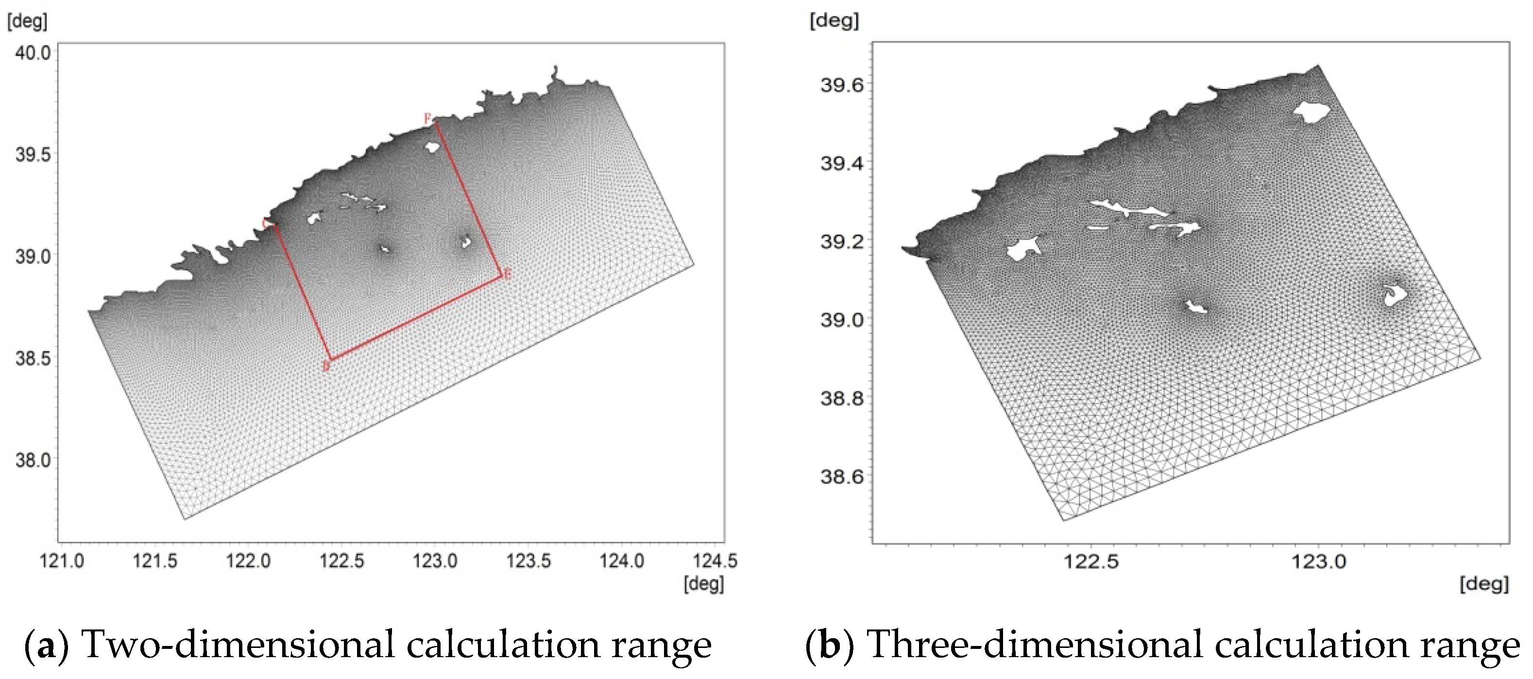
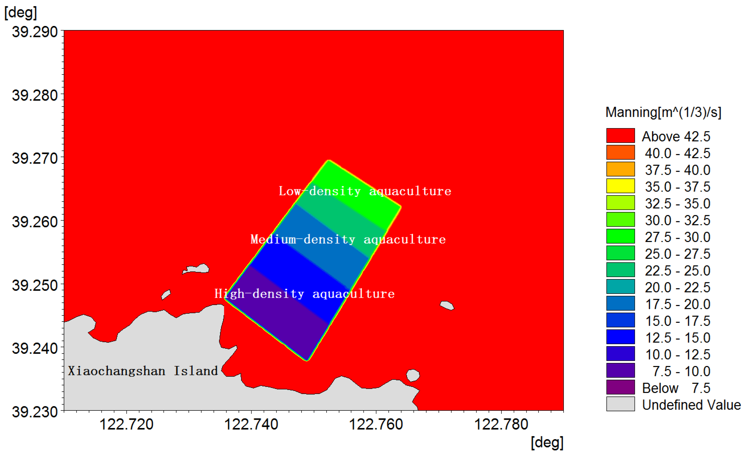
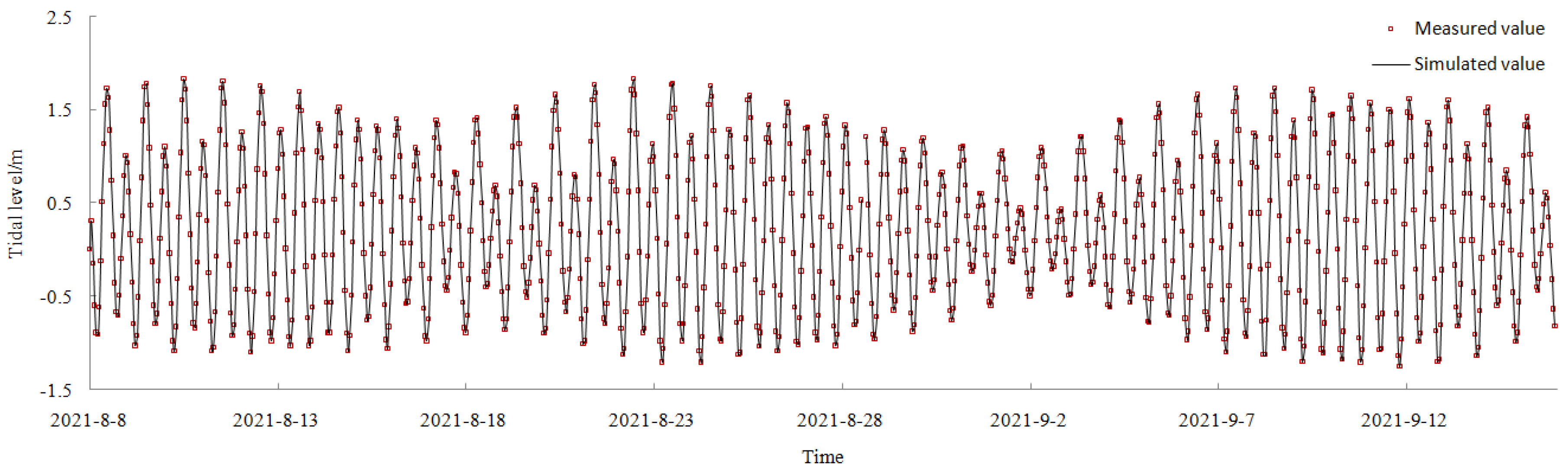
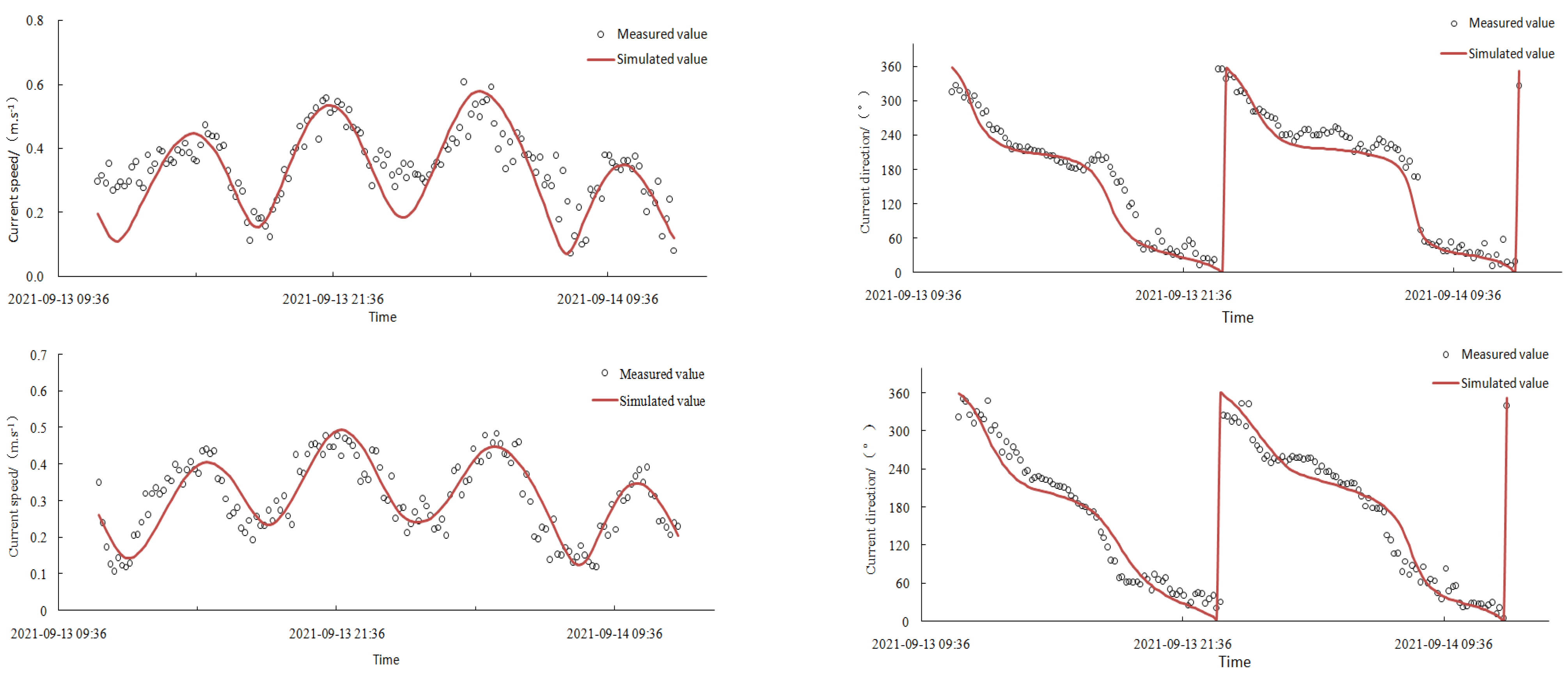
The original intention of this work was to solve some problems with floating raft aquaculture areas. In this study, a typical floating raft aquaculture area located in Changhai County, Liaoning Province, was chosen as the research area on the basis of the successful establishment of the hydrodynamic model and tracer model in these area of Liaodong Bay, in order to quantitatively explain the impact of floating raft aquaculture on the hydrodynamic environment of an open sea area. Compared with the sea area of Liaodong Bay, the study area features a higher degree of openness. Aiming to comprehensively understand the temporal and spatial distribution and variation characteristics of hydrodynamic force in the waters near the floating raft aquaculture area located in Changhai County, Dalian, the project team simulated and analyzed the hydrodynamic field and water exchange rate in the sea area near the floating raft aquaculture area. In this study, depth-averaged two-dimensional shallow-water equations and three-dimensional incompressible Reynolds-averaged Navier–Stokes equations were established for the open sea area. We described the impact of rafts (floaters, ropes, cages, cultured organisms, etc.) on hydrodynamic force in the aquaculture area by changing the Manning number of the seabed. Finally, the model was verified with the observed hydrodynamic data, and the results show that the model has great accuracy, stability, and universality, and it can provide an accurate prediction of the hydrodynamic environment of aquaculture in the raft area.

2. Materials and Methods

2.1. Observational Data

The project team set up a temporary tide-level observation station, T1, in the coastal waters of Dalian, and conducted tide-level observations for three months, from 00:00, 1 August 2021 to 23:00, 31 October 2021. Two continuous observation stations, P1 and P2, were set up for ocean current observation, where a total of 25 h of layered and synchronous continuous ocean current observations were carried out, from 11:00, 13 September 2021 to 12:00, 14 September 2021. The specific coordinates of the stations are shown in

Table 1. Coordinates of the hydrometric stations for hydrological tide tests.

Station	Longitude	Latitude
T1	121°41.12′ E	38°52.08′ N
P1	123°6.098′ E	39°7.111′ N
P2	123°12.539′ E	39°10.895′ N

, and their locations are shown in Figure 2. Refer to Section 3.1 for the specific observation values below.

2.2. Model and Methods

The model is based on the solution of the three-dimensional incompressible Reynolds-averaged Navier–Stokes equations. First, the integration of the horizontal momentum equations and the continuity equation over depth for the following two-dimensional shallow water equations was carried out [13,14,15,16]. Based on the aforesaid principle, the commercial model encapsulation platforms used in this study mainly included Hydro info, a water conservancy information system developed by Dalian University of Technology, China, and Mike, a commercial water simulation computing system developed by the Danish Hydraulic Institute (DHI).

Based on the above model and methods, the specific implementation process was completed, as follows. First, in order to accurately analyze the hydrodynamic conditions of the water area near Changhai County, two-dimensional models of the Yellow Sea and the Bohai Sea and the waters near Changhai County were created, where the open boundary of an open water area was driven by the time series file of the tidal level. Then, in order to reflect the hydrodynamic conditions of the sea area near the aquaculture area located in Changhai County in more detail, a three-dimensional model of a small area of interest in Changhai County was created with a nesting method [17,18] based on the tidal-level drive after the calibration of the two-dimensional model of Changhai County, where the calculation range mainly covered the area contained by the four control points C, D, E, and F shown in

Table 2. Coordinates of points in the range of the calculation domain.

Point	Longitude	Latitude
C	122.1380° E	39.1450° N
D	122.4400° E	38.4820° N
E	123.3560° E	38.8970° N
F	122.9990° E	39.6470° N

, and the locations of the control points are shown in Figure 3a.

2.2.1. Hydrodynamic Model

The study area is located along the northern coast of the Yellow Sea (see Figure 1), where tidal currents play a dominant role in various flow components. The three-dimensional Navier–Stokes equations for the free-surface flow of incompressible fluid in the Cartesian coordinate system were used for description; on this basis, the horizontal momentum equations and the continuity equation for the three-dimensional shallow water form were integrated in the range H = η + h to obtain the following depth-averaged two-dimensional shallow water continuity equation:

$$\frac{\partial \eta }{\partial t}+\frac{\partial }{\partial x}(hu)+\frac{\partial }{\partial y}(hv)=0$$

(1)

Momentum equations

$$\frac{du}{dt}-\frac{\partial }{\partial x}\left({\gamma }^h\frac{\partial u}{\partial x}\right)-\frac{\partial }{\partial \mathrm{y}}\left({\gamma }^{{}_h}\frac{\partial u}{\partial y}\right)-fv+\frac{gu\sqrt{u^2+v^2}}{C_Z{}^{2}H}=-g\frac{\partial \eta }{\partial x}$$

(2)

$$\frac{dv}{dt}-\frac{\partial }{\partial x}\left({\gamma }^{{}_h}\frac{\partial v}{\partial x}\right)-\frac{\partial }{\partial \mathrm{y}}\left({\gamma }^h\frac{\partial v}{\partial y}\right)+fu+\frac{gv\sqrt{u^2+v^2}}{C_Z{}^{2}H}=-g\frac{\partial \eta }{\partial y}$$

(3)

where η represents the sea surface fluctuation (tidal level) relative to the still sea surface; h represents the still water depth (the distance from the seabed to the still sea surface); H = η + h represents the total water depth; C_z = n. H^(1/6) is the Chezy coefficient; n = 1/M is Manning’s roughness coefficient, and M represents the Manning number.

Equations (1)–(3) are the basic governing equations for solving the hydrodynamic elements. In order to comply with the uniqueness of solutions, the definite conditions must be given.

(1)

Initial Conditions

The cold-start mode was used, meaning that the initial conditions were considered irrelevant to the final result of the calculation. In this study, the initial flow rate and tidal level were both determined as 0.

(2)

Boundary Conditions

For the numerical model used in this study, two boundary conditions need to be given, including open boundary and closed boundary conditions. For a tidal flat near the island coastline, the position of the land–water interface changed with the fluctuation of the tide level, and the dry–wet variation of the grid nodes in the moving boundary was taken into consideration in this work [19,20,21].

① Open boundary condition:

The open boundary condition is also known as the water boundary condition, where, on this boundary, either the flow rate is given, or the time series condition of the tidal level is given. For the open boundary in this work, calculation was performed in the following form of tidal harmonic analysis:

$${\eta }_i={\displaystyle \sum _i^m{f}_i{H}_i\cos [{\omega }_{i}t+{(V_0+u)}_i-g_i]}$$

(4)

where ω_i represents the angular velocity of the ith tidal constituent; f_i and u represent the intersection factor and epoch correction of the ith tidal constituent, respectively; H_i and g_i represent harmonic constants, which are the amplitude and epoch of each tidal constituent, respectively; V₀ represents the time angle of a tidal constituent. The time series data of the tide level at the open boundary of the model were also verified according to the global tide module.

② Closed boundary condition:

The normal flow rate at the shoreline of the given water body should be 0.

2.2.2. The Euler Model for Residual Current Calculation

As the most important environmental dynamic factor in coastal waters, the residual current plays a crucial role in the transport and diffusion of substances in seawater. In studies on ocean dynamics, Eulerian velocity is usually used to calculate residual currents. The Euler residual current in the ocean can be simply defined as the mean Eulerian velocity, which can be calculated with the following equation:

$$U_E=\frac{1}{nT}{\displaystyle {\int }_{t_0}^{t_0+nt}u\left(x_0,t\right)}dt, V_E=\frac{1}{nT}{\displaystyle {\int }_{t_0}^{t_0+nt}v\left(x_0,t\right)}dt$$

(5)

where U_E and V_E represent the mean Eulerian velocities in directions x and y, respectively; n represents the number of cycles used in the calculation; t₀ represents the start time of calculation; T represents the current cycle; u(x₀,t) and v(x₀, t) represent the component velocities in directions x and y. The numerically discrete form of Equation (6) is described below:

$$U_E=\frac{1}{N}{\displaystyle \sum _{i=1}^N{u}_i}, V_E=\frac{1}{N}{\displaystyle \sum _{i=1}^N{v}_i}$$

(6)

where N = nT/Δt and Δt represent the time step of numerical simulation.

2.2.3. Mathematical Model of Water Exchange

The tracer method was used to simulate the degree of water exchange [22,23,24], where a dissolved non-degradable and conservative substance was set in the sea area, and its concentration diffusion under the action of hydrodynamic force was investigated. For the transport of the tracer, the convection–diffusion equation based on Eulerian substance transport was used, as shown below:

$$\frac{\partial hC}{\partial t}+\frac{\partial huC}{\partial x}+\frac{\partial hvC}{\partial y}=\frac{\partial }{\partial x}\left(h{D}_x\frac{\partial C}{\partial x}\right)+\frac{\partial }{\partial y}\left(h{D}_y\frac{\partial C}{\partial y}\right)-FhC+S$$

(7)

where C represents the substance concentration; D_x and D_y represent the substance diffusion coefficients in directions x and y, respectively; F represents the substance attenuation coefficient, which is zero (F = 0) for the conservative substance; S represents the point source concentration.

The substance diffusion coefficient was calculated with the following equation:

$$D_x=\frac{E_x}{{\sigma }_T}; D_y=\frac{E_y}{{\sigma }_T}$$

(8)

where E_x = E_y represents the horizontal turbulent viscosity coefficient; σ_T represents the Prandtl number, which was determined as 1.0 in this study.

After a certain period of time, the percentage of the total amount of substance diffused from the system to open water divided by the total amount of initial substances in the system should be the water exchange rate of the overall system. The statistical calculation expression is provided below.

$$EX(t_j)=\left(1-\frac{{\displaystyle \sum _{i=1}^N{C}_i(t_j)H_i(t_j)}}{{\displaystyle \sum _{i=1}^N{C}_i(t_0)H_i(t_0)}}\right)\times 100\%$$

(9)

where EX represents the water exchange rate; C represents the substance concentration; H represents the total water depth; i represents the node number in the statistical domain; n represents the total number of nodes in the statistical domain; j represents the time number.

2.3. Grid Creation and Parameter Setting

2.3.1. Grid Creation

The calculation grid was generated with the Surface Water Model System(SMS 10.1). This grid generation program can realize a flexible and variable resolution in the horizontal direction of the grid and a large gradient, and it can create a highly smooth grid at a location where a flow tends to be generated around an island. In addition, it can partially increase the density in areas with complex terrain, such as coastal areas, estuaries, and wetlands.

The entire two-dimensional simulated domain of Changhai County consists of 32,560 nodes and 63,579 triangular elements. Figure 3a shows the calculation domain and grid distribution of the established two-dimensional model of the sea area near Changhai County. The entire simulated domain of the three-dimensional model [25] consists of 12,539 nodes and 24,281 triangular elements. Figure 3b shows the calculation domain and grid distribution of the three-dimensional model of a small area of Changhai County.

2.3.2. Model Calculation Settings

(1)

The calculation of hydrodynamic force

The calculation time step of the model was adjusted according to the CFL conditions to ensure that when the model calculation was converged, the minimum time step was 5.0 s. The seabed friction was controlled by the Manning number, with a specific value of 32–42 m^1/3/s. In many applications, a constant eddy viscosity can be used for the horizontal stress terms. Alternatively, Smagorinsky proposed to express sub-grid-scale transport by effective eddy viscosity related to a characteristic length scale. The sub-grid-scale eddy viscosity is given in [26], and the specific expression is shown below:

$$A=c_{{}_s}^2{l}^2\sqrt{2S_{ij}{S}_{ij}}$$

(10)

where c_s is a constant; l is a characteristic length; and the deformation rate is given by

$$S_{ij}=\frac{1}{2}\left(\frac{\partial u_i}{\partial x_j}+\frac{\partial u_j}{\partial x_i}\right)$$

(11)

The minimum calculation time step of the three-dimensional small-scale local model was 1.0 s. In the vertical grid, the sigma hierarchical function was adopted, and the impact of the rafts on the hydrodynamic force was described with a double-resistance model with the introduction of a secondary drag coefficient, where the frictional resistance of the seabed was controlled by secondary drag coefficient C_f, and the specific expression was determined by assuming a logarithmic profile between the seabed and a point at a distance of DZ_b above the seabed as follows:

$${\mathrm{C}}_{\mathrm{f}}=[\frac{1}{\kappa }\ln \left(\frac{D{Z}_b}{Z_0}\right){]}^{-2}$$

(12)

where $\kappa =0.4$ is the von Kármán constant; Z₀ represents the length scale of the roughness of the riverbed; when the boundary surface is rough, Z₀ depends on the roughness height, where Z₀ = mk_s, the approximate value of m is 0.033, k_s is the roughness height, ranging between 0.01 m and 0.30 m, and the value was determined as 0.05 m. In summary, the average value of the secondary drag coefficient was 0.01.

(2)

The calculation for the aquaculture area

The location of the selected aquaculture area, the range of the calculation domain, and the distribution of the seabed topography are shown in Figure 1. The aquaculture area is located in a sea area near the Changshan Archipelago in the southeast of Changhai County, and its boundaries are shown in

Table 3. Scope of the aquaculture area.

Longitude	Latitude
122.7492° E	39.2382° N
122.7642° E	39.2585° N
122.7527° E	39.2697° N
122.7363° E	39.2480° N

below.

In the post-aquaculture model, unstructured grids were also used to divide the horizontal calculation domain and locally densify the sea area where the aquaculture area was located, with a grid scale of 30 m. In other areas along the shoreline, the grid scale ranged between 50 m and 100 m; in sea areas far away from the aquaculture area, the maximum grid scale was 400 m, and the calculation domain contained 17,642 triangular grids and 9011 nodes. The Manning field considering aquaculture areas of different densities is shown in Figure 4 below.

(3)

Assessment of water exchange capacity

In this study, the water exchange rate was used as an index to describe the water exchange capacity of the aquaculture area. A dissolved conservative substance was placed in the sea area where the aquaculture area was located, which would be carried by the water body and could not be degraded. The convection and diffusion of the conservative matter directly reflect the form of movement of the water body. Based on the above considerations, in this study, a conservative substance with a concentration of 1.0 was placed in the aquaculture area; the concentration of substances in open water was set at 0.0; the attenuation coefficient was set as F = 0, and the point source concentration was set as S = 0. The substance diffusion coefficient was equal to the turbulent viscosity coefficient of water flow (σ_T = 1.0).

3. Results

3.1. Model Verification Results

The actual calculation and simulation period of the model was from 0:00, 1 August 2021 to 23:00, 31 October 2021. Figure 5 shows a time-curve-based comparison between the simulated and measured values of the tidal level during the period from 0:00, 8 August 2021 to 23:00, 15 September 2021. Figure 6 shows the comparison between P1 and P2 in terms of flow rate, flow direction, and measured value during the period from 11:20, 13 September 2021 to 12:30, 14 September 2021. To fully represent the calculation results of the numerical model, Figure 7 shows the flow rates and flow direction fields of the top, middle, and bottom layers at the same moment during a spring tide and a neap tide in the three-dimensional calculation model for Changhai County.

A comparison between Figure 5 and Figure 6 shows that the results calculated by the model are in good agreement with the measured values, where the error is within an acceptable range. According to the verification results of tidal currents and the flow field distribution maps at different moments, as shown in Figure 5, the mathematical model can reflect the flow field in the sea area near Changhai County in a more realistic manner, indicating that the model has reasonable boundaries and parameters and can be used for the calculation of subsequent working conditions. Figure 6 indicates that the trends of variation in the simulated flow rate and flow direction are generally the same as those of the measured values, where the measured maximum flow rates of P1 and P2 during 13 September and 14 September are 0.606 m/s and 0.491 m/s, respectively, and the simulated maximum flow rates are 0.577 m/s and 0.493 m/s, respectively. In general, the simulated calculated values are in good agreement with the measured values. Figure 7 shows that although grids of different scales were used in the calculation of the two-dimensional and three-dimensional models, the flow rate and flow direction in the entire spatial calculation domain reasonably changed, featuring a strong gradient and no sudden change, which indicates that the model is stable and can be used as the basis for the calculation of subsequent working conditions.

In order to verify the accuracy, the root-mean-square error (R) was used to quantitatively analyze the error between the calculation results of the model and the measured values, where R represents the mean deviation between the results of the model and the observed data. R is calculated as follows:

$$R=\sqrt{\frac{{\displaystyle {\sum }_{i=1}^n{\left(M_i-O_i\right)}^2}}{n}}$$

(13)

where M_i represents the calculated value of the model; O_i represents the observed value; and n represents the number of observed values. After calculation, the root-mean-square error in the tidal level of T1 is less than 0.18 m, generally indicating that the simulated value is in good agreement with the measured value, and the model has great accuracy and reliability.

Tracer model verification is indeed a relatively important part of the assessment of water exchange capacity, which has been verified in other studies [27,28], as described below. In these studies, one of the major tasks was the numerical simulation of the transportation of water pollutants in Liaodong Bay, the northernmost bay in the Bohai Sea in China. On the basis of a comprehensive understanding of the natural conditions of the sea area of Liaodong Bay, the impact of point source input was introduced to establish a convection-diffusion model for pollutant transport in the sea area of Liaodong Bay, with which the distribution of different nutrient elements in the sea area was simulated, and where major water quality indicators included NH₃-N and COD. The accuracy and stability of the model were verified through a comparison between the simulated values and the concentration levels of the elements obtained by field sampling and analysis in the sea area, indicating that the model features a great ability to reproduce and predict the concentration field in the sea area of Liaodong Bay. In respect of the following few years, the distribution of PO4-P, a water quality indicator, in Liaodong Bay, was reproduced, and model verification was performed, providing the simulation results of the hydrodynamic field, half exchange time, and concentration field in Liaodong Bay at different typical moments. Finally, this model was adopted in the simulation and assessment for the identification of marine pollution accidents, and it delivered satisfactory results.

3.2. Simulation Results of Tidal Current and Residual Current in the Aquaculture Area

The results regarding the distribution of the flow field in the sea area near the aquaculture area are shown in Figure 8, Figure 9, Figure 10 and Figure 11, indicating that the flow field in the aquaculture area exhibits the characteristics of reciprocating motion, where the main flow direction is NW–SE, and the flow rate magnitude during a flood tide and an ebb tide is 1.0 m/s. In accordance with the simulation result of the hydrodynamic field in the sea area of Changhai County, the Euler residual current field in the sea area near the aquaculture area was obtained. Figure 12 shows the Euler residual current fields in the cycle of a spring tide before and after the implementation of aquaculture activities, indicating that the mean residual current intensity in the aquaculture area was approximately 0.018 m/s; the direction was NE; and there was generally no significant variation before and after the implementation of aquaculture activities.

In order to quantitatively and clearly reflect the impact of surface roughness (Manning) on the calculation results, the sensitivity of the Manning number was analyzed. For the sea area near the floating raft aquaculture area, which is 180–3650 m from the shoreline, the simulated values of flow rate and flow direction at the peak of a flood tide and at the peak of an ebb tide during a spring tide in one tidal cycle were compared before and after the implementation of aquaculture, where the Manning settings under the two working conditions were as shown in Part 2. The results show that the changes in flow rate and flow direction were generally significant in the study area, especially during the flood tide, wherein the flow rate changed by more than 80% within 750 m in the aquaculture area; the mean change in flow rate was approximately 10%, and the number of points where the flow direction changed by more than 45° accounted for around 20% of the total number. This indicates that, after the establishment of aquaculture activities, as the Manning number of the aquaculture area decreased and the roughness increased, which, together with the effect of flow resistance arising from the raft net, indeed significantly affected the flow rate and flow direction of the sea area near the aquaculture area.

3.3. Simulation Results of Water Exchange Rate

Based on the aforesaid hydrodynamic simulation results, a mathematical model of water exchange, described in Equations (7)–(9), was used to study the water exchange capacity of the aquaculture area. In addition, in order to enable the model to reflect the variation in water exchange capacity before and after the implementation of aquaculture activities in a clearer and more sensitive manner, the scope of the aquaculture area was appropriately magnified according to the actual sea area, and the calculation domain and grid were rearranged and refined, where the average grid scale was 50 m, and the minimum grid scale for the key areas of interest in the aquaculture area was 30 m.

Figure 13 and Figure 14 show the initial field distribution of the tracer concentration distribution, and the overall water exchange rate–time curves before and after the implementation of aquaculture activities, respectively.

Table 4. Statistics for the water exchange rate–time curves before and after the implementation of aquaculture.

Working Condition/Time	0 d	1 d	2 d	4 d	6 d	8 d
Before the implementation of aquaculture activities	0	27.90%	47.95%	61.83%	69.71%	76.48%
After the implementation of aquaculture activities	0	22.90%	39.05%	53.43%	66.04%	75.23%

shows the statistics for the overall water exchange rate–time curves before and after the implementation of aquaculture activities, indicating that the water exchange rate after the implementation of aquaculture decreased compared with that before implementation. Before the implementation of aquaculture, the water exchange rates after 1, 4, and 8 days of water exchange were 27.90%, 61.83%, and 76.48%, respectively; after the implementation of aquaculture, the water exchange rates after 1, 4, and 8 days of water exchange were 22.90%, 53.43%, and 75.23%, respectively.

4. Discussion

4.1. Tidal Current Conditions

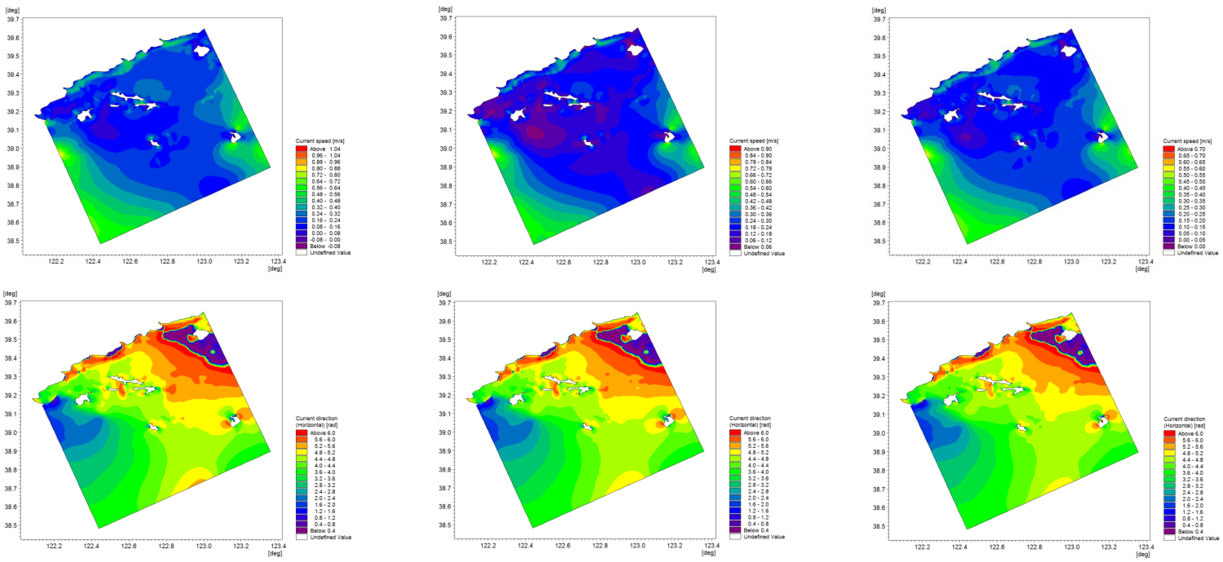
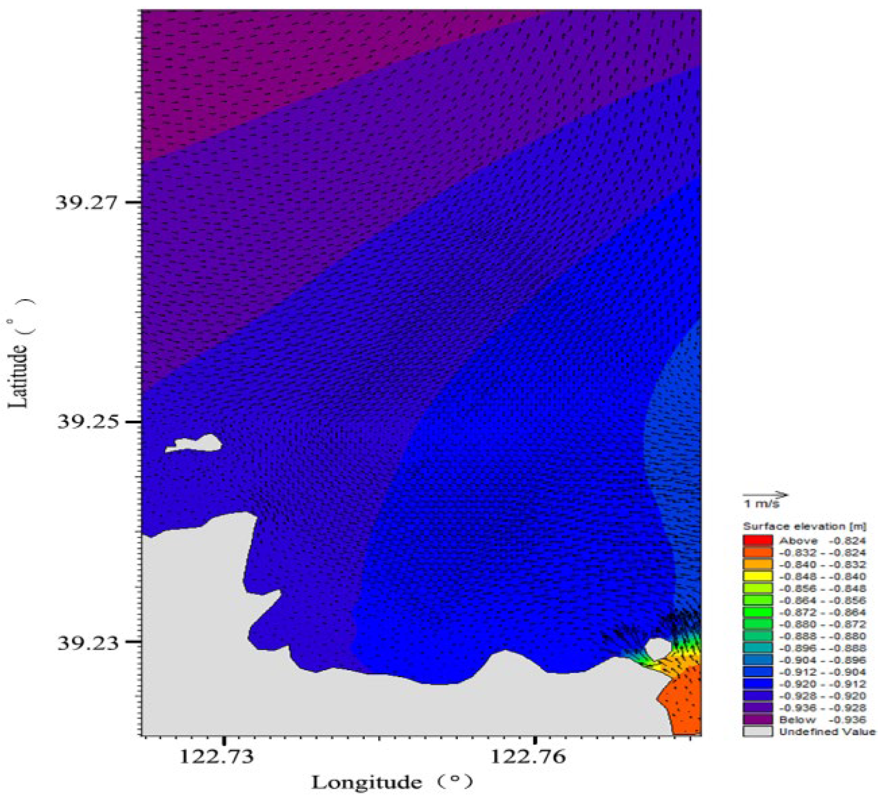
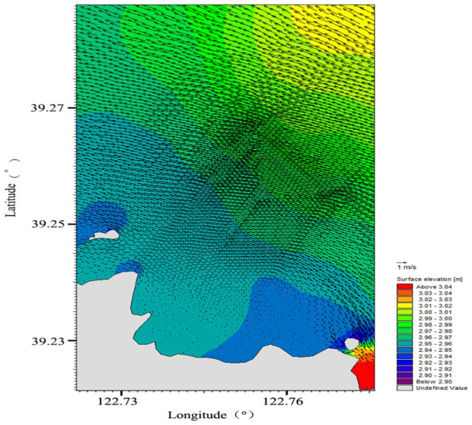
The hydrodynamic force calculation results indicate that the hydrodynamic force in the waters near Changhai County is mainly in the NW–SE direction during a spring tide, during which the tidal currents of flood and ebb tides rotate counterclockwise. During the spring tide, the tidal field shows that the tidal direction in the open waters of Changhai County was NW, the tidal field was stable, and the flow rate generally ranged between 0.50 m/s and 0.85 m/s. The nearshore current is a coastal current in essentially the same direction as the shoreline and has a lower flow rate, ranging between 0.2 m/s and 0.4 m/s. This is mainly because the flow rate is significantly reduced by the bottom friction due to the shallow water in the near-shore area. The local coastal waters are affected by the coastline, with a maximum flow rate of 1.2 m/s during a flood tide; during an ebb tide, the flow direction in the open waters is SE, and the flow rate ranges between 0.45 m/s and 0.90 m/s. Affected by the topography, coastal waters generally feature lower flow rates, with a maximum flow rate of approximately 1.1 m/s.

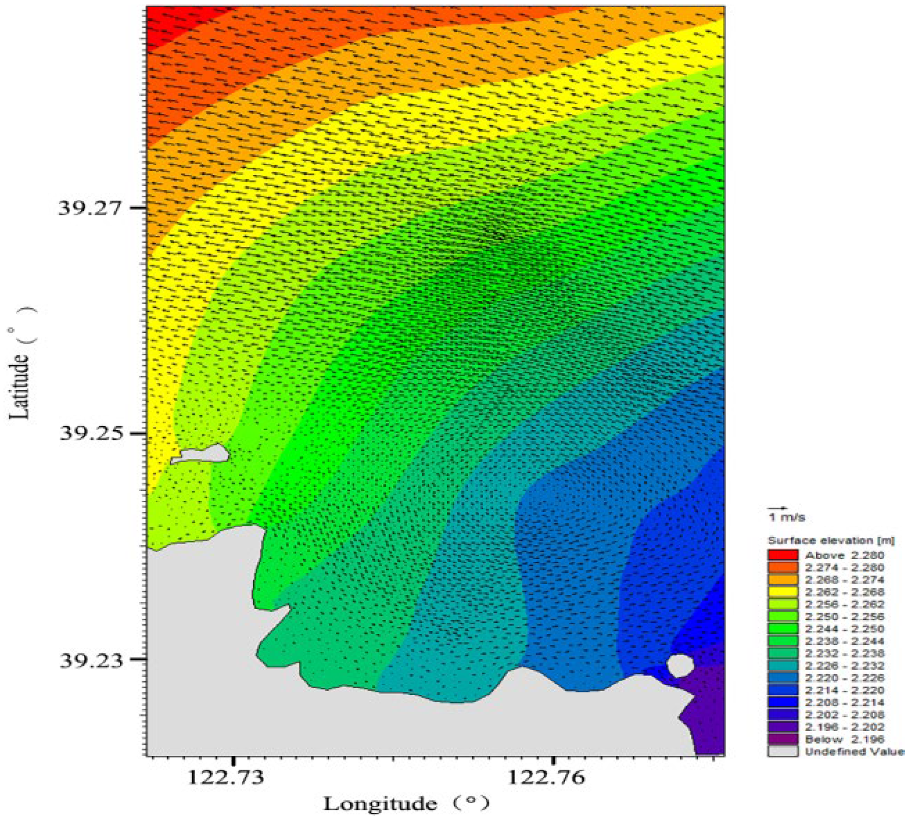
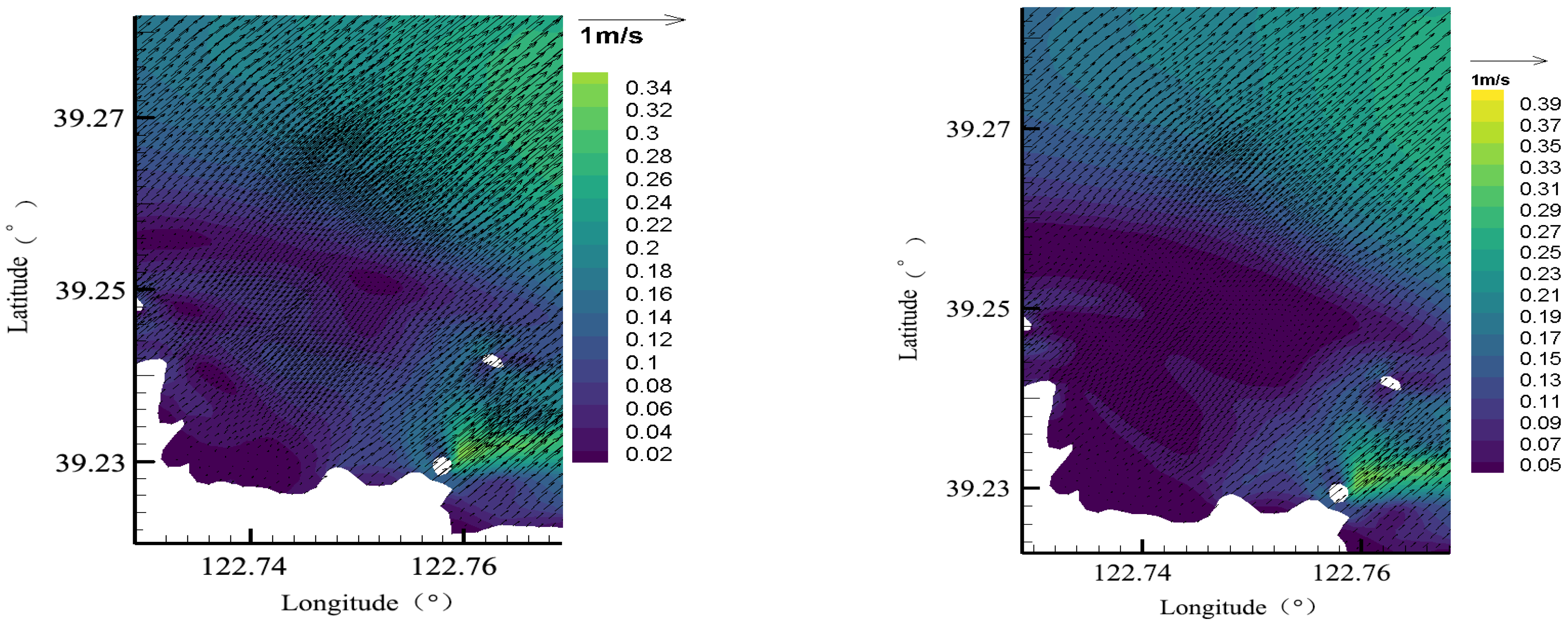
4.2. Conditions of the Aquaculture Area

The calculation of the characteristics of the flow rate in the aquaculture area shows that flow rates in the aquaculture area usually range between 0.2 m/s and 0.4 m/s. There is a small island in the SE direction in the aquaculture area, so the maximum flow rate in the aquaculture area is up to 0.7 m/s; the flow rate gradually increases from the shoreline to the sea, and it reaches 1.0 cm/s in the part of the aquaculture area that is closer to the shoreline. A comparison with the flow rate before the implementation of aquaculture activities shows that, with regard to the degree of flow resistance imposed by the floating rafts, the variation in flow rate ranges between 2.87% and 84.58% at the peak of a flood tide, and between 2.65% and 20.89% at the peak of an ebb tide from a low-density zone to a high-density zone of the aquaculture area. This indicates that the variation in flow rate caused by the floating rafts in the sea area near the aquaculture area of Changhai County is significantly greater during a flood tide than that during an ebb tide, and the flow resistance rate at the peak of a flood tide is greater than 80%. Therefore, aquaculture operators and marine environmental protection workers should pay attention to the impact of floating rafts for aquaculture. Even in open sea areas, during the setting of the orientation and density of a floating raft aquaculture area, it is crucial to first investigate the hydrodynamic conditions and the impact of aquaculture activities on the hydrodynamic conditions in the sea area, in order to scientifically implement aquaculture activities and rationally determine the layout while protecting the marine environment.

4.3. Residual Current Conditions

Residual current distribution plays a decisive role in the transport and diffusion of bait, nutritive salts, and other related substances in an aquaculture area. According to a comparison with the residual current before the implementation of aquaculture activities, the extent of variation ranged between 3.01% and 84.74% during a spring tide, and it ranged between 9.46% and 78.50% during a neap tide, indicating that the extents of variation in residual current during tides are essentially the same; they should not be underestimated. Therefore, to accurately understand the distribution of algae and bait in the floating raft aquaculture area, we must calculate and analyze the residual current in the sea area based on accurate hydrodynamic analysis. In this way, we can understand the characteristics of the transport and diffusion of floating and suspended substances in the sea area in real time, thereby providing guidance for the formulation of aquaculture plans and production activities.

4.4. Water Exchange Conditions

The quantitative calculation shows that, due to the aquaculture activities, the water exchange rates of the open sea area decreased by 17.92%, 13.59%, and 1.63% compared with those before implementation; moreover, the half-exchange cycle of the water body appeared in 2.3 d and 3.9 d, respectively, before and after the implementation of aquaculture. This indicates that even floating rafts for aquaculture located in an open sea area have a certain impact on the water exchange capacity, and the specific extent of such impact is closely related to various factors, such as the density, size, scope, and location of rafts in the aquaculture area.

5. Conclusions

In this study, a numerical simulation method was applied to a floating raft aquaculture sea area to quantitatively calculate and assess the changes in the hydrodynamic environment of the open sea area. The model is based on the solution of the three-dimensional incompressible Reynolds-averaged Navier–Stokes equations. Then, the integration of the horizontal momentum equations and the continuity equation over depth for the two-dimensional shallow water equations was carried out. In the hydrodynamic model, in order to generalize the impact of rafts on the hydrodynamic force in the aquaculture area, the Manning number of the seabed—namely the seabed roughness—in the two-dimensional mode was changed; in the three-dimensional mode, a double-resistance model of the top and bottom layers was used, with the introduction of a secondary drag coefficient. The final verification and results show that the numerical model proposed in this paper can satisfactorily simulate and predict the hydrodynamic conditions of the sea area near the aquaculture area in Changhai County; the three-dimensional flow field can reflect the variation in the spatially stratified hydrodynamic indexes of the dynamic environment in a more realistic way, which can also reflect the hindering effect of rafts on hydrodynamic force in a more accurate way, and the model features great accuracy and stability. According to the working conditions before and after the implementation of aquaculture activities, the impact of the floating rafts on the hydrodynamic environment and water exchange capacity was compared and analyzed. The results indicate that the flow resistance rate was greater than 80%; the maximum decrease in the water exchange rate was close to 20%. The quantitative results sufficiently show that, even if floating rafts are arranged with a certain density in a completely open sea area, they have a great impact on the hydrodynamic conditions of the sea area. Therefore, aquaculture operators and marine environmental protection workers must pay sufficient attention to the impact of floating rafts for aquaculture on the hydrodynamic conditions of sea area. The establishment of the method in this paper provides a basic model for the rational arrangement of a fully open raft aquaculture area and the scientific determination of breeding density, and it offers a quantitative numerical calculation method for the assessment of the water exchange capacity in aquaculture areas containing flexible objects [29] (such as rafts, vegetation, etc.).It also provides aquaculture operators with technical support in making scientific and effective decisions regarding aquaculture.

In future studies, spatial modeling for floating rafts, mainly including floaters, external aquaculture nets for hanging cages and organisms, will be added, and a fluid–structure interaction-based multiphase flow (volume of fluid, VOF) model will be used to simulate the impact of floating rafts for aquaculture on the dynamic environment and water exchange, in order to provide more accurate and comprehensive technical support for the rational arrangement of aquaculture orientation and the scientific setting of aquaculture density. Furthermore, after the accurate determination of the impact of a raft aquaculture area on the hydrodynamic conditions, it is also possible for aquaculture operators to reasonably select a site for the installation of bait casting and distribution devices, which can thus help to considerably increase the production efficiency of raft aquaculture, guarantee a stable income for aquaculture operators, and improve the social and economic benefits of raft aquaculture in sea areas in Changhai County and even in other open sea areas with floating raft aquaculture.

References

1. Zhao, Y.; Zhang, J.; Liu, Y.; Sun, K.; Zhang, C.; Wu, W.; Teng, F. Numerical assessment of the environmental impacts of deep sea cage culture in the Yellow Sea, China. Sci. Total Environ. 2019, 706, 135752.1–135752.10. [Google Scholar] [CrossRef] [PubMed]
2. Klebert, P.; Patursson, O.; Endresen, P.C.; Rundtop, P.; Birkevold, J.; Rasmussen, H.W. Three-dimensional deformation of a large circular flexible sea cage in high currents: Field experiment and modeling. Ocean Eng. 2015, 104, 511–520. [Google Scholar] [CrossRef]
3. Dong, S.; You, X.; Hu, F. Experimental investigation on the fluid–structure interaction of a flexible net cage used to farm Pacific bluefin tuna (Thunnus orientalis). Ocean Eng. 2021, 226, 1–12. [Google Scholar] [CrossRef]
4. Dong, S.; Park, S.; Kitazawa, D.; Zhou, J.; Yoshida, T.; Li, Q. Model tests and full-scale sea trials for drag force and deformation of a marine aquaculture net cage. Ocean Eng. 2021, 240, 1–17. [Google Scholar] [CrossRef]
5. Klebert, P.; Su, B. Turbulence and flow field alterations inside a fish sea cage and its wake. Appl. Ocean. Res. 2020, 98, 1–15. [Google Scholar] [CrossRef]
6. Ji, R.B.; Mao, X.H.; Zhu, M.Y. The impact of shellfish aquaculture on the gulf ecosystem. J. Oceanogr. Huanghai Bohai Seas 1998, 1, 21–27. [Google Scholar]
7. Hatcher, A.; Grant, J.; Schofield, B. Effects of suspended mussel culture (Mytilus spp.) on sedimentation, benthic respiration and sediment nutrient dynamics in a coastal bay. Mar. Ecol. Prog. Ser. 1994, 115, 219–235. [Google Scholar] [CrossRef]
8. Bouchet, V.M.P.; Sauriau, P. Influence of oyster culture practices and environmental conditions on the ecological status of intertidal mudflats in the Pertuis Charentais (SW France): A multi-index approach. Mar. Pollut. Bull. 2008, 56, 1898–1912. [Google Scholar] [CrossRef] [Green Version]
9. Panchang, V.; Cheng, G.; Newell, C. Modeling Hydrodynamics and Aquaculture Waste Transport in Coastal Maine. Estuaries 1997, 20, 14–41. [Google Scholar] [CrossRef]
10. Fan, X.; Wei, H.; Yuan, Y.; Zhao, L. Vertical structure of tidal current in a typically coastal raft-culture area. Cont. Shelf Res. 2009, 29, 2345–2357. [Google Scholar] [CrossRef]
11. Duarte, P.; Alarez-Salgado X., A.; Fernandez-Reiriz, M.J.; Piedracoba, S.; Labarta, U. A modeling study on the hydrodynamics of a coastal embayment occupied by mussel farms (Ria de Ares-Betanzos, NW Iberian Peninsula). Estuar. Coast. Shelf Sci. 2014, 147, 42–55. [Google Scholar] [CrossRef]
12. Jie, S.; Hao, W. Numerical simulation of the hydrodynamic field in a semi-enclosed high-density raft aquaculture sea area. Period. Ocean Univ. China 2009, 39, 1181. [Google Scholar]
13. Shi, F.; Dong, X. Three-dimension numerical simulation for vulcanization process based on unstructured tetrahedron mesh. J. Manuf. Process. 2016, 22, 1–6. [Google Scholar] [CrossRef]
14. Zhang, P.; Zhang, R.J.; Huang, J.M.; Sheng, Z.; Wang, S. FVCOM model-based study on tidal prism and water exchange capacity of Haizhou Bay. Water Resour. Hydropower Eng. 2021, 52, 143–151. [Google Scholar]
15. Chen, C.S.; Liu, H.D.; Beardsley, R.C. An unstructured grid, finite-volume, three-dimensional, primitive equations ocean model: Application to coastal ocean and estuaries. Atmos. Ocean. Technol. 2003, 20, 159–186. [Google Scholar] [CrossRef]
16. Zhao, C.; Ren, L.; Yuan, F.; Zhang, L.; Jiang, S.; Shi, J.; Chen, T.; Liu, S.; Yang, X.; Liu, Y.; et al. Statistical and Hydrological Evaluations of Multiple Satellite Precipitation Products in the Yellow River Source Region of China. Water 2020, 12, 3082. [Google Scholar] [CrossRef]
17. Zhao, S.; Jin, S.; Ai, C.; Zhang, N. Visual analysis of three-dimensional flow field based on WebVR. J. Hydroinformat. 2019, 21, 671–686. [Google Scholar] [CrossRef]
18. Casulli, V.; Walters, R.A. An unstructured grid, three dimensional model based on the shallow water equations. Int. J. Numer. Methods Fluids 2000, 32, 331–348. [Google Scholar] [CrossRef]
19. Minhaz, F.A.; Mazlin, B.M.; Chen, K.L.; Nuriah, A.M. Identification of Water Pollution Sources for Better Langat River Basin Management in Malaysia. Water 2022, 14, 1904. [Google Scholar]
20. Liu, X.; Ma, D.G.; Zhang, Q.H. A higher-efficient non-hydrostatic finite volume model for strong three-dimensional free surface flows and sediment transport. China Ocean. Eng. 2017, 31, 736–746. [Google Scholar] [CrossRef]
21. Stanovoy, V.V.; Eremina, T.R.; Isaev, A.V.; Neelov, I.A.; Vankevich, R.E.; Ryabchenko, V.A. Modeling of oil spills in ice conditions in the Gulf of Finland on the basis of an operative forecasting system. Marine Phys. 2012, 52, 754–759. [Google Scholar] [CrossRef]
22. Wang, S.; Zhang, P.; Xi, Y.B.; Ding, J.; Han, Y.; Zhang, R. Study on the effect of culturing floating raft on water exchange capacity in Haizhou Bay. Water Resour. Hydropower Eng. 2021, 52, 109–120. [Google Scholar]
23. Shi, J.; Wei, H.; Zhao, L.; Yuan, Y.; Fang, J.; Zhang, J. A physical–biological coupled aquaculture model for a suspended aquaculture area of China. Aquaculture 2011, 318, 412–424. [Google Scholar] [CrossRef]
24. Bilgili, A.; Proehl, J.A.; Lynch, D.R.; Smith, K.W.; Swift, M.R. Estuary/ocean exchange and tidal mixing in a Gulf of Maine Esturay: A Lagrangian modeling study. Estuar. Coast. Shelf Sci. 2005, 65, 607–624. [Google Scholar] [CrossRef]
25. Park, J.C.; Kim, M.H.; Miyata, H. Filly nor linear free-surface simulations by a 3D viscous numerical wave tank. Int. J. Numer. Methods Fluids 1999, 29, 685–703. [Google Scholar] [CrossRef]
26. Smagorinsky, J. General circulation experiments with the primitive equations: I. The basic experiment. Mon. Weather Rev. 1963, 91, 99–164. [Google Scholar] [CrossRef]
27. Wang, K.; Wang, N.B. Numerical Simulation of Water Pollutant Transport in Liaodong Bay. J. Hydrodyn. 2010, 25, 493–498. [Google Scholar]
28. Wang, K.; Guo, N.; Wang, N.; Leng, C.; Wang, Z.; Li, A.; Xu, X. Simulation of water exchange capacity in Liaodong Bay and application of conservative water quality model. Fish. Sci. 2013, 32, 475–481. [Google Scholar]
29. Wang, C.; Zhu, P.; Wang, P.F. Effects of aquatic vegetation on flow in the Nansi Lake and its flow velocitymodeling. J. Hydrodyn. 2006, 18, 640–648. [Google Scholar] [CrossRef]
Figure 1. Location and scope of the aquaculture area.
Water 14 03125 g001
Figure 2. Locations of the observation stations.
Water 14 03125 g002
Figure 3. Calculation ranges and grid distribution maps of the models.
Water 14 03125 g003
Figure 4. Distribution of Manning field after the implementation of aquaculture activities.
Water 14 03125 g004
Figure 5. Tidal-level verification map of T1.
Water 14 03125 g005
Figure 6. Verification of flow rates and directions at P1 and P2.
Water 14 03125 g006
Figure 7. Flow field distribution maps of the top, middle, and bottom layers during a spring tide in the three-dimensional calculation domain of a small area of Changhai County.
Water 14 03125 g007
Figure 8. Flow field distribution at high tide.
Water 14 03125 g008
Figure 9. Flow field distribution at low tide.
Water 14 03125 g009
Figure 10. Flow field distribution at the peak of an ebb tide.
Water 14 03125 g010
Figure 11. Flow field distribution at the peak of a flood tide.
Water 14 03125 g011
Figure 12. Residual current distribution in the sea area near the aquaculture area ((left): before aquaculture; (right): after aquaculture).
Water 14 03125 g012
Figure 13. Tracer concentration distribution at the initial time point (the red area is the statistical area for water exchange rate).
Water 14 03125 g013
Figure 14. Water exchange rate–time curves before and after the implementation of aquaculture.
Water 14 03125 g014