Perennial Groundwater Zone Formation Processes in Thin Organic Soil Layers Overlying Thick Clayed Mineral Soil Layers in a Small Serpentine Headwater Catchment

Abstract

Groundwater zone formation in the soil layers of a headwater catchment is an important factor that controls volumetric and chemical changes in streamflow; it also induces shallow landslides. Previous studies have suggested that the groundwater zone in soil layers generally forms transiently atop low-permeability layers in response to rainfall. This study focused on an unchanneled hollow in a serpentine headwater catchment, where a semi-perennial to perennial groundwater zone was observed in thin organic soil layers (OSLs) overlying thick clay mineral soil layers (CMLs), even during dry periods. We conducted detailed observations in this catchment to clarify the formation processes of the semi-perennial to perennial groundwater zone. The results showed that water is supplied from the CMLs to the OSLs as unsaturated upward flow in areas where the OSLs are dry. This water then accumulates in the downslope hollow, which sustains the groundwater zone in the OSLs during dry periods. The frequent and long-term occurrence of upward flow can be attributed to differences in the hydraulic properties of OSLs and CMLs. This process prevents the OSLs in the hollow from drying, presumably causes volumetric and chemical changes in streamflow, and reduces the stability of OSLs.

1. Introduction

The groundwater zone within the soil layers of a headwater catchment has been recognized as one of the most important factors controlling volumetric [1,2,3] and chemical [4,5] changes in streamflow and in the induction of shallow landslides [6,7]. Clarification of the formation process of the groundwater zone within soil layers is needed to predict changes in streamflow and the occurrence of shallow landslides. Based on numerous studies involving detailed field observations in various headwater catchments, including the Maimai catchment, New Zealand [8,9,10,11]; Walker Branch watershed, U.S.A. [12]; LI1 catchment at Llyn Brianne, Wales [13]; and Hitachi Ohta experimental watershed, Japan [14], the formation process of the groundwater zone can be described as follows. Rainwater vertically infiltrates into permeable soil layers. This water reaches low-permeability layers (i.e., bedrock) and flows laterally along their surfaces, transiently forming a groundwater zone above low-permeability layers in the downslope area. This groundwater zone shrinks through the discharge of water into streams after rainfall has ceased; it generally disappears (especially in small catchments) during dry periods because of the low capacity of a small headwater catchment to store water, combined with high permeability of soil layers.

Although this formation process is widely accepted in various headwater catchments, some studies have identified a groundwater zone within the soil layers, even during dry periods. Frisbee et al. [15] observed groundwater table dynamics in two hillslope transects and calculated the water balance for them. They reported that during periods of low water table position, large-volume groundwater storage was observed in a depression located near the base of the slope that maintained streamflow. Such depressions formed atop less permeable layers are presumed to increase water storage, thereby preventing the groundwater zone from drying up. Fujimoto et al. [16] conducted hydrological observations on two types of hillslopes (valley head and side slope) in a headwater catchment; they demonstrated that the hillslope with highly convergent topography continued to sustain wet conditions through the concentration of subsurface water during dry periods. These studies highlighted the importance of hillslope topography in maintaining the groundwater zone during dry periods. Moreover, although bedrock groundwater is commonly reported to exfiltrate into channels and thus influence stream discharge and quality during baseflow periods [17,18,19], some studies that included detailed hydrological, hydrochemical, and hydrothermal observations have shown that bedrock groundwater can also exfiltrate into soil layers, thereby generating a perennial groundwater zone in the soil layers. Uchida et al. [20] indicated that expansion and contraction of the groundwater zone in a soil layer at a slope base during periods of normal low flow and drought were controlled by bedrock groundwater exfiltration. Katsura et al. [21] found that a groundwater zone was present within the soil layers at a slope base in a headwater catchment during dry periods; they demonstrated that the groundwater zone was maintained by bedrock groundwater exfiltration. Thus, water flow from bedrock can contribute to the formation of a groundwater zone in the soil layer during dry periods.

In this study, we observed groundwater dynamics in a small headwater catchment (0.068 ha) with gentle topography underlain by serpentine. In this catchment, a semi-perennial to perennial groundwater zone forms in thin, high-permeability organic soil layers (OSLs) in an unchanneled hollow; it remains present during dry periods. The small catchment area, lack of a large depression, low topographic convergence, and presence of thin OSLs with high permeability in this catchment suggest that the effects of catchment topography cannot explain the observed semi-perennial to perennial groundwater zone in the OSLs. A substantial contribution from bedrock groundwater exfiltration is also unlikely due to the presence of mineral soil layers that consist of thick clay mineral layers (CMLs) with low permeability above the bedrock, which inhibit bedrock groundwater flow into the OSLs. Thus, the aforementioned formation processes of a groundwater zone in soil layers, which were based on observations in catchments with no thick clay mineral layers, cannot explain the semi-perennial to perennial groundwater zone observed in this catchment. The groundwater zone observed in this catchment appeared to be controlled by another factor. Using hydrometric, hydrochemical, and thermal observations, this study explored the formation process of the semi-perennial to perennial groundwater zone observed in the OSLs of this catchment.

2. Materials and Methods

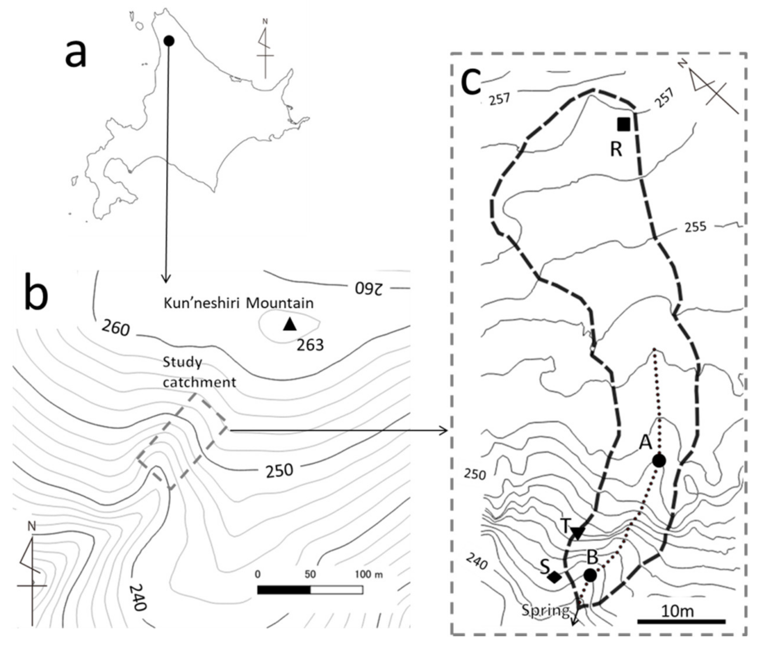
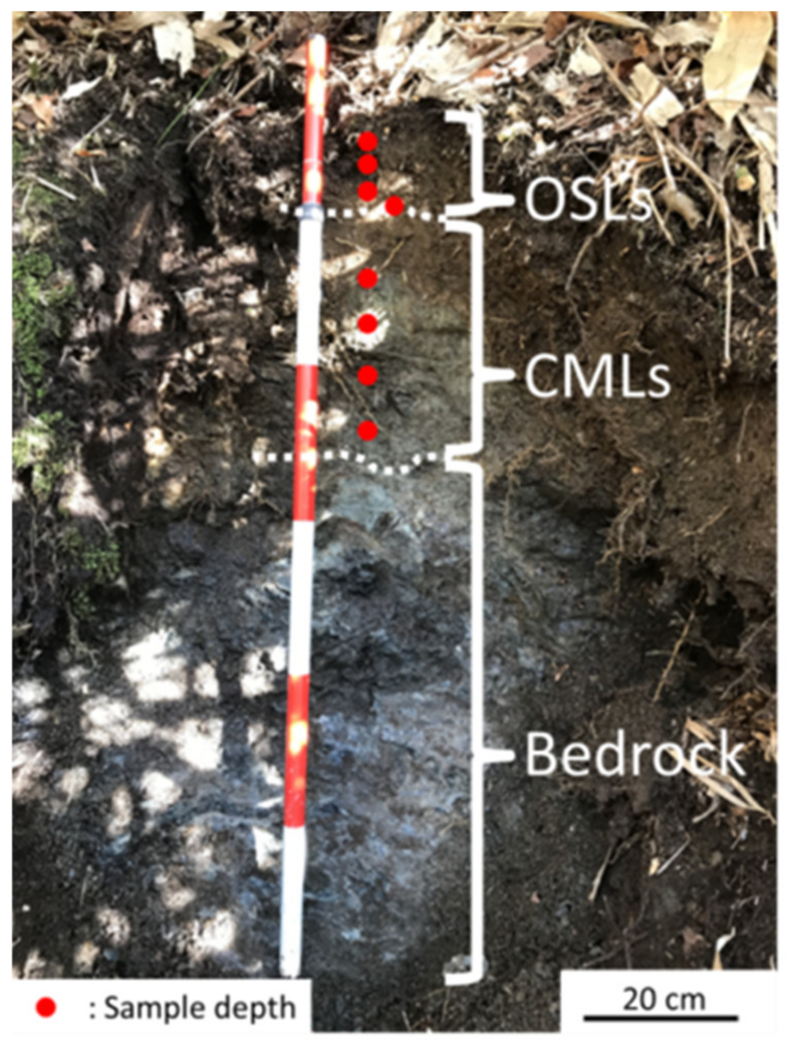
2.1. Study Site

The study was conducted in a very small forested headwater catchment (0.068 ha; 44°52′ N, 142°4′ E) on Kunneshiri Mountain in Nakagawa Experimental Forest, which is managed by Hokkaido University and located in Hokkaido, northern Japan (Figure 1). The elevation of the catchment ranges from 241 to 257 m above sea level (Figure 1c), and a spring is present at the catchment outlet. The region has a mean annual temperature of 5.9 °C (1989–2019) and precipitation of 1240 mm (1989–2019) according to data from the nearest weather station (the Japan Meteorological Agency Automated Meteorological Data Acquisition System [(AMeDAS) Nakagawa observation station, located approximately 5 km south-southwest of the catchment). The snowfall season in Nakagawa Experimental Forest is from late November through late April or early May [22], and the maximum snow depth during this season is about 1.7 ± 0.5 m [23]. The dominant tree species in Nakagawa Experimental Forest are Abies sachalinensis, Picea glehnii, Picea jezoensis, Sorbus commixta, Quercus crispula, and Acer pictum [24]; the understory is densely covered with Sasa kurilensis and Sasa senanensis [25].

The study catchment is underlain by serpentinite bedrock and features low elevation, gentle hillslopes, and a rounded ridge with a mean gradient of 14°. These topographic characteristics are consistent with the characteristics of other serpentinite catchments in Japan [26]. The surface soil type of the area underlain by serpentine is “Wet Iron Podzol” [27]. In this catchment, OSLs are very thin, with thickness ranging from 10 to 50 cm. Mineral soil layers derived from weathering of the serpentinite bedrock consist of clayey materials (referred to as CMLs in this study), with thickness ranging from 30 to 170 cm. Each layer is thicker in the middle of the slope and thinner in the upper and lower parts. Whereas macropores and pipes can form within CMLs and contribute to preferential flow in catchments with geological settings other than serpentinite [28,29], they are not observed in the study catchment because the CMLs consist of stiff clayey materials and the high concentration of nickel in serpentine soils inhibits root growth into the CMLs [30].

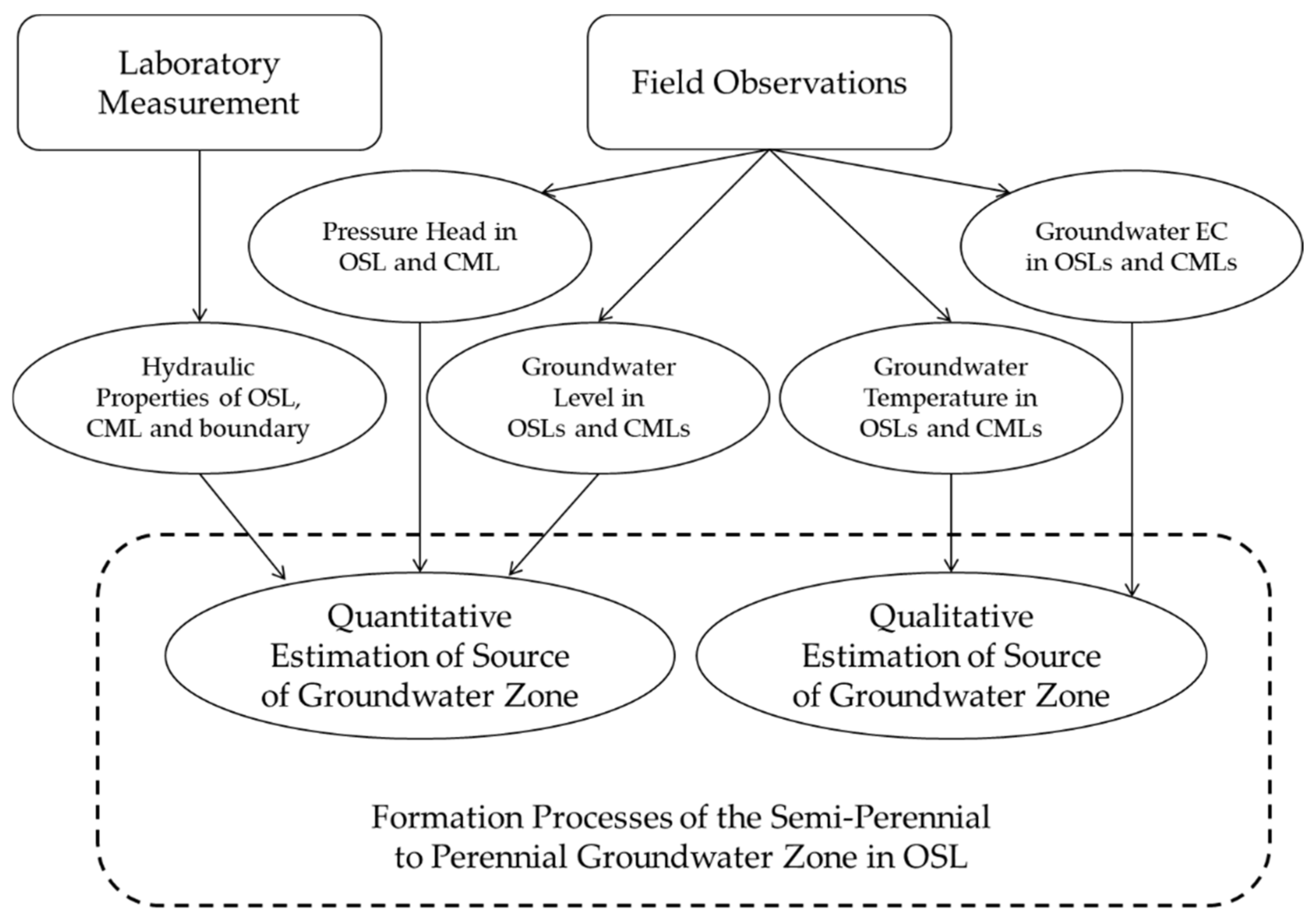
2.2. Laboratory Measurement

Figure 2 shows a flowchart of the methodology used to explore the formation process of the semi-perennial to perennial groundwater zone observed in the OSLs of this catchment. First, to measure the hydraulic properties of OSLs, CMLs, and the boundary layers between them, we collected undisturbed core samples (100 cc in volume) from a trench (Figure 3) excavated at Point S in Figure 1c. The thicknesses of the OSL and CML at this point are 10 and 33 cm, respectively. In total, three, one, and four samples were collected from the OSL, boundary layer, and CML, respectively. We confirmed that the soil and bedrock structure at this point is almost the same as the structure at other points (e.g., Points A, B, and T; mentioned later). Moreover, the area of the study catchment is very small (0.068 ha). Hence, we assumed that the collected samples were representative of each layer in the catchment.

We conducted water retention tests on all core samples in the laboratory. To obtain and characterize water retention curves for each sample, we fitted a lognormal model [31] to the observed relationship between volumetric water content, $\theta$, and pressure head, $\psi$ (cm). The lognormal model was derived by applying the lognormal distribution law to the soil pore radius distribution function, and the water retention curve is expressed as follows:

$$S_e=\frac{\theta -{\theta }_r}{{\theta }_s-{\theta }_r}=Q\left(\frac{ln\left(\psi /{\psi }_m\right)}{\sigma }\right)$$

(1)

where S_e represents the effective saturation; ${\theta }_s$ and ${\theta }_r$ are the saturated and residual volumetric water contents, respectively; ${\psi }_m$ is the pressure head at $S_e=0.5$; $\sigma$ is a dimensionless parameter characterizing the width of the pore-size distribution; and Q is the complementary normal distribution function:

$$Q\left(x\right)={{\displaystyle \int }}_x^{\infty }\frac{1}{\sqrt{2x}}\exp \left(-\frac{u^2}{2}\right)du$$

(2)

We determined the values of ${\theta }_r$, ${\psi }_m$, and $\sigma$ for each sample through minimization of the residual sum of squares, which was obtained from the measured and calculated values of $\theta$ at the applied $\psi$, with ${\theta }_s$ fixed at the measured value. Finally, the mean water retention curves of OSLs and CMLs were obtained using the mean parameter values of core samples collected from each layer (arithmetic means of ${\theta }_s$, ${\theta }_r$, and $\sigma$; geometric mean of ${\psi }_m$). The water retention curve for the OSL–CML boundary zone was obtained using parameter values determined from the OSL–CML boundary core sample.

We also measured the saturated hydraulic conductivity, $K_s$, for all core samples in the laboratory. The hydraulic conductivity curve was obtained using the model proposed by Kosugi [31]. The following functional relationship between hydraulic conductivity, $K$, and $\psi$ was obtained by combining Equation (1) with Mualem’s [32] model:

$$K\left(\psi \right)=K_s{S}_e{}^{1/2}{\left[Q\left(\frac{ln\left(\psi /{\psi }_m\right)}{\sigma }+\sigma \right)\right]}^2$$

(3)

Mean hydraulic conductivity curves for OSLs and CMLs were obtained using the geometric mean value of $K_s$ for core samples collected from each layer with the mean parameter values of ${\psi }_m$ and $\sigma$, which were determined as described above. The hydraulic conductivity curve for the OSL–CML boundary was obtained using the measured value of $K_s$ and the parameter values of ${\psi }_m$ and $\sigma$.

2.3. Field Observations

Temporal variations of $\psi$ were measured at Point T (Figure 1c) at 60 min intervals from 15 May to 1 November 2019 using tensiometers. We selected this point because it is located at the catchment boundary in the downslope area and therefore roughly represents the average degree of wetness for the whole catchment. The OSL depth is 31 cm at this location. The tensiometer installation depths were 30 (in the OSLs), 50, and 80 cm (in the CMLs).

To separately monitor groundwater levels and temperature in the OSLs and CMLs, two pairs of observation wells (for OSLs and CMLs) were manually excavated at Points A and B along an unchanneled hollow in the study catchment (Figure 1c). All wells were constructed using 6 cm diameter polyvinyl chloride pipes perforated with numerous 5 mm diameter holes. The depths of the wells for observation of the OSLs at Points A and B (equivalent to the depths to the CML surfaces at each point) were 41 and 38.5 cm, respectively. The depths of the wells for the CMLs at Points A and B were 209 and 164 cm (equivalent to the depths of the bedrock surfaces at each point), respectively. To prevent groundwater in the OSLs from directly infiltrating into the CML wells, the upper sections of the CML wells were unperforated. The depth of the unperforated section was 60 cm at Point A and 43 cm at Point B; it was greater than the OSL depth at each point. A water-level gauge with a temperature recorder was installed at the bottom of each observation well, where it measured the groundwater level and temperature simultaneously at 60 min intervals from 15 May to 1 November 2019.

For analysis of electrical conductivity (EC; μS cm⁻¹), water samples were collected at intervals of approximately 4–5 weeks from mid-May through early November 2019. Samples of groundwater in the OSLs and CMLs were collected directly from the wells. Rainwater samples were collected using a plastic bottle equipped with a mesh-covered 21-cm-diameter funnel located at Point R in a clearing in the study catchment (Figure 1c). The measured EC values were converted to values at a standard temperature of 25 °C.

All rainfall and air temperature data were obtained from the Japan Meteorological Agency AMeDAS Nakagawa observation station.

3. Results

3.1. Hydraulic Properties

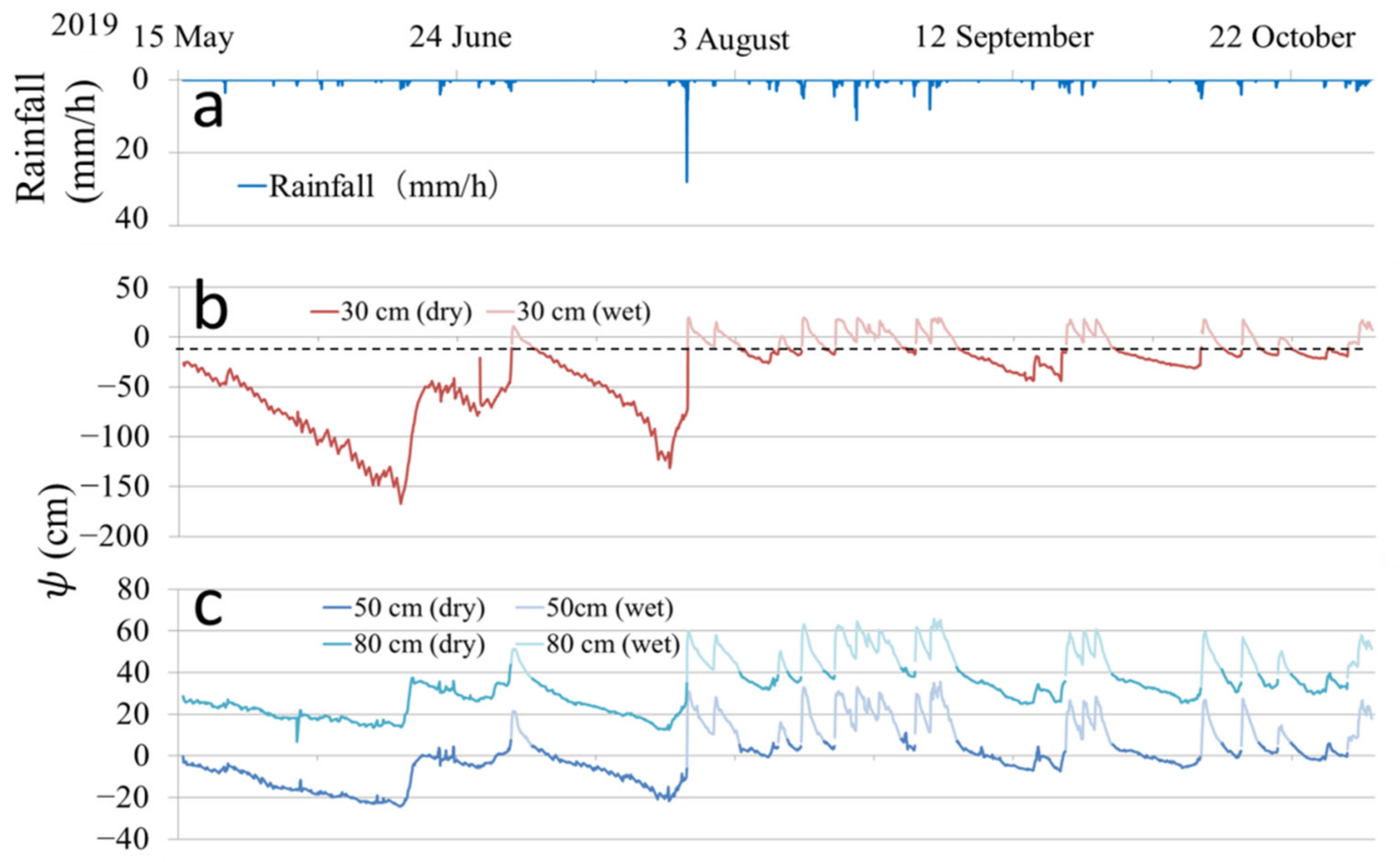
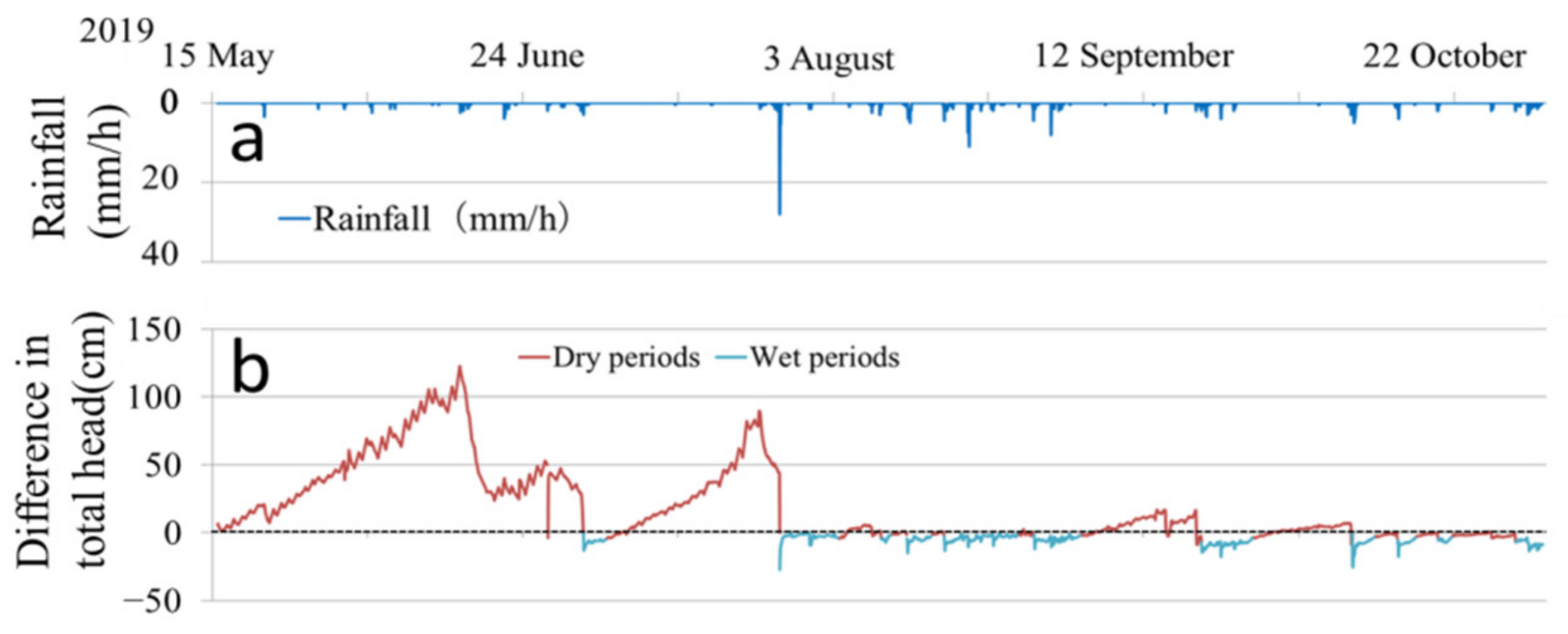
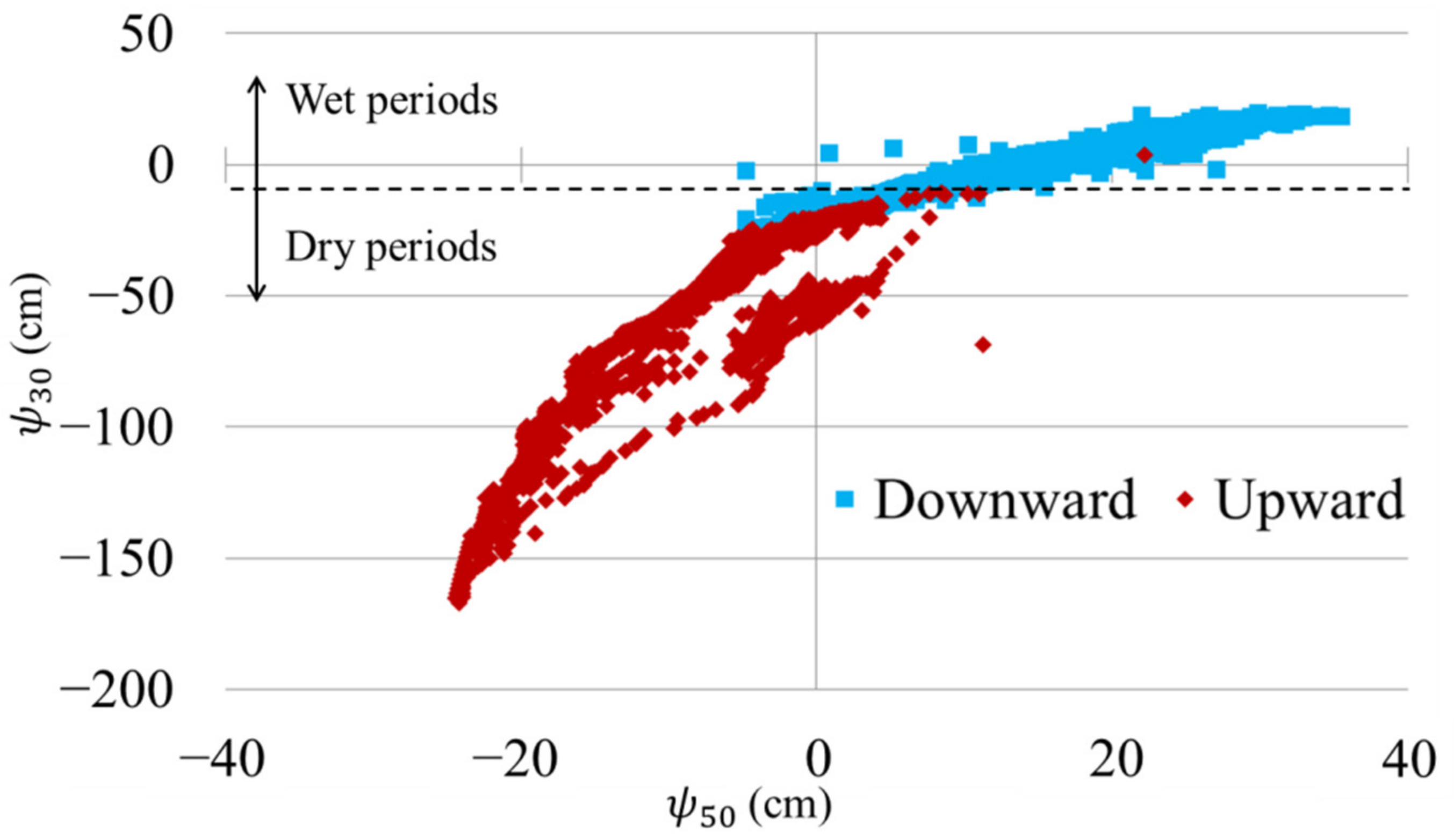
Figure 4 shows the water retention and hydraulic conductivity curves of the OSLs, CMLs, and boundary layer. The parameter values are listed in

Table 1. Parameter values for hydraulic properties.

	$K_s$ cm s−1	${\theta }_s$	${\theta }_r$	${\psi }_m$ cm	$\sigma$
OSLs	3.38 × 10−2 a	0.707 b	0.250 b	−303.4 a	3.05 b
CMLs	6.76 × 10−4 a	0.549 b	0.374 b	−303.2 a	2.10 b
Boundary	2.14 × 10−2	0.718	0.442	−200.3	2.67

Note(s): ^a Geometric mean. ^b Arithmetic mean.

. The $\theta$ value of the OSLs is large at $\psi$ = 0 cm (i.e., ${\theta }_s$ = 0.707); it shows a sharp and continuous decrease (approximately 0.204) as $\psi$ decreases to −200 cm (Figure 4a). The decrease in $\theta$ is most prominent in the wet range of $\psi$ > −10 cm (0.060). In contrast, $\theta$ in the CMLs is smaller at $\psi$ = 0 cm (${\theta }_s$ = 0.549) than in the OSLs; it decreases less sharply (0.074) from ${\theta }_s$ as $\psi$ decreases to −200 cm, with no prominent decrease in the wet range. Because ${\theta }_s$ is equivalent to the total volume of soil pores and water drains earlier from larger pores than from smaller pores as $\psi$ decreases, these water retention curves suggest that the OSLs contain many pores of various sizes from very large (as indicated by the prominent change in $\theta$ in the wet range) to small, whereas the CMLs have only a few large pores. The $\theta$ value of the OSL–CML boundary is similar to the $\theta$ value of OSLs at $\psi$ = 0 cm (${\theta }_s$ = 0.718), and it shows an intermediate rate of decrease (0.138) as $\psi$ decreases to −200 cm.

The measured $K_s$ values of the OSLs ranged from 1.07 × 10⁻² to 6.06 × 10⁻² cm s⁻¹, with a geometric mean of 3.38 × 10⁻² cm s⁻¹; these values were larger than the $K_s$ of CMLs, which ranged from 2.37 × 10⁻⁴ to 6.08 × 10⁻³ cm s⁻¹, with a geometric mean of 6.76 × 10⁻⁴ cm s⁻¹ (Table 1). Figure 4b depicts hydraulic conductivity curves for the OSLs, CMLs, and OSL–CML boundary; it shows that the $K$ of the OSLs rapidly decreases from 3.38 ×10⁻² cm s⁻¹ to 2.34 × 10⁻⁵ cm s⁻¹ as $\psi$ decreases from 0 to −10 cm. In contrast, the reduction in the $K$ values of CMLs across the same $\psi$ range is smaller (6.76 × 10⁻⁴ cm s⁻¹ to 6.58 × 10⁻⁵ cm s⁻¹). Therefore, although OSLs have a larger $K_s$ ($K$ at $\psi$ = 0 cm) than CMLs, OSLs have a smaller $K$ than CMLs in the range of $\psi$ < −1.5 cm ($K$ < 3.00 × 10⁻⁴ cm s⁻¹). At the OSL–CML boundary, $K$ decreases from 2.14 × 10⁻² to 7.50 × 10⁻⁵ cm s⁻¹ as $\psi$ decreases from 0 to −10 cm. In the range of $\psi$ < −10 cm, OSLs, CMLs, and the OSL–CML boundary all show gentler changes in $K$ than in the range of $\psi$ > −10 cm.

3.2. Pressure Head

Figure 5 shows hourly rainfall and $\psi$ in the OSL (30 cm depth) and CMLs (50 and 80 cm depths) at Point T. Total precipitation during the study period was 468.5 mm. Positive and negative $\psi$ values indicate saturated and unsaturated conditions, respectively. The OSLs showed a rapid increase in $\psi$ and often reached saturation in response to rainfall, whereas periods without rainfall resulted in $\psi$ decreases and severe drying. Careful examination of Figure 5b demonstrates that $\psi$ in the OSL displayed a rapid decrease from saturation to approximately −10 cm, followed by a gentler decrease as $\psi$ decreased further. This tendency can be attributed to the water retention curve of OSLs (Figure 4a). The observed rapid decrease in $\psi$ from saturation to $\psi$ = −10 cm presumably reflects rapid drainage of water through very large pores. Based on the tendencies described here, we defined wet and dry periods in this study as periods with OSL $\psi$ of >−10 cm and <−10 cm, respectively. The variations of $\psi$ are shown in Figure 5b, c for wet and dry periods, respectively. The 80 cm sampling depth in the CMLs showed smaller $\psi$ responses to rainfall and was constantly saturated in both wet and dry periods. The 50 cm sampling depth in the CMLs became saturated in response to rainfall and gradually returned to unsaturation after rainfall ceased. The $\psi$ fluctuated less at 50 cm than at 30 cm (in the OSLs); it remained close to saturation even when $\psi$ values at depths upward of 20 cm indicated severely dry conditions. These $\psi$ dynamics indicate wetter conditions in the CMLs than in the OSLs, especially during dry periods.

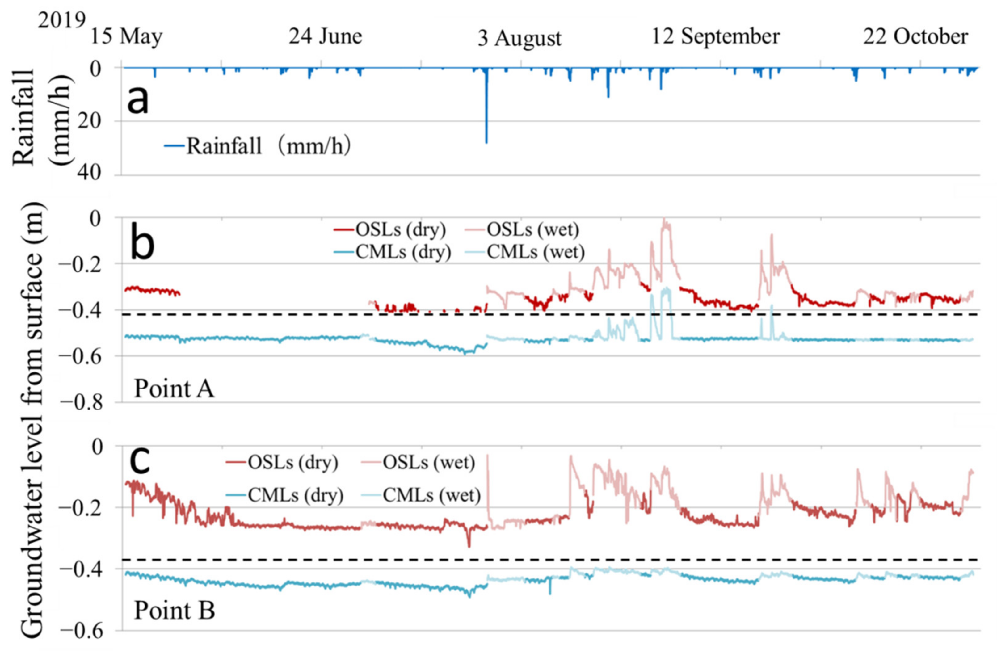
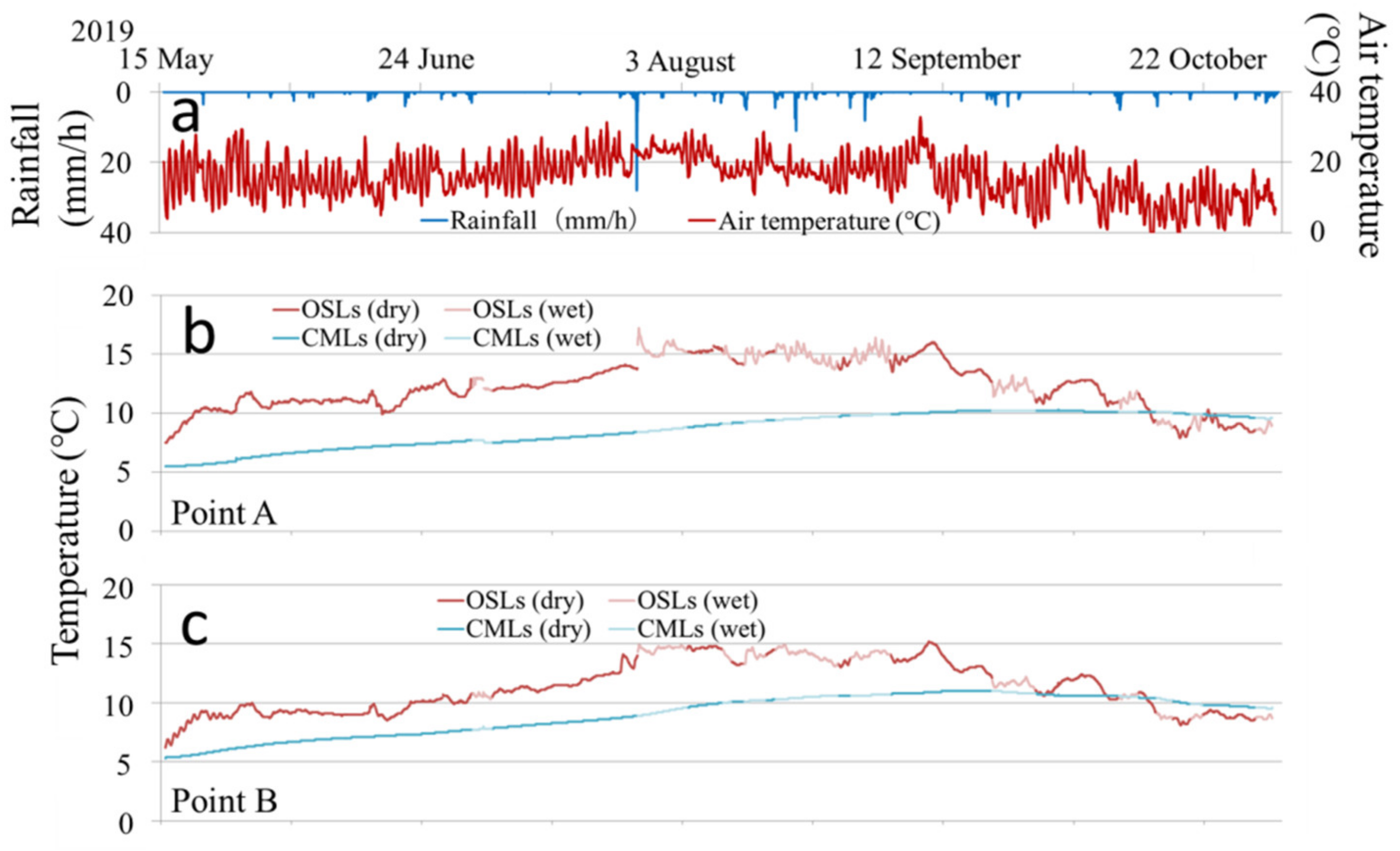
3.3. Groundwater Level and Temperature

Figure 6 shows hourly rainfall and the groundwater level in the OSLs and CMLs at Points A and B. The groundwater level is presented as the depth below the ground surface, and the OSL–CML boundary is denoted with a dashed line. In the study catchment, we observed two distinct groundwater levels, in OSLs and CMLs (OSL groundwater and CML groundwater, respectively). Observation data for OSL groundwater at Point A are missing because of equipment failure from 26 May at 13:00 through 3 July at 10:00.

At Point A, the OSL groundwater showed rapid fluctuations in response to rainfall; it was present throughout the observation period except in July, when low precipitation and high evapotranspiration during the summer drought period in Hokkaido [33] caused the groundwater level to intermittently decrease to zero (Figure 6b). Notably, OSL groundwater was sustained from 2 September through 17 September despite extremely low rainfall (5.0 mm) during this period. In contrast, the CML groundwater level was less responsive to rainfall. The CML groundwater level generally did not reach the OSL–CML boundary, although a few rainfall events increased the CML groundwater level above the OSL–CML boundary. Even during such periods, the CML groundwater level did not match the OSL groundwater level, suggesting distinct groundwater zones in the OSLs and CMLs. The minimum groundwater level in the CMLs was −0.593 m, which was observed on 22 July at 16:00 during the drought period; this level was 0.183 m below the boundary.

At Point B, the groundwater level in the OSLs was observed continuously; it showed steep increases and decreases in response to rainfall (Figure 6c). Excluding the rapid decrease and recovery of the groundwater level within the OSLs from 23 July at 1:00 to 14:00 during the summer drought period, the minimum groundwater level was −0.282 m on 17 July at 16:00 (in a dry period), which was 0.103 m above the boundary; this finding indicated that groundwater was permanently present at approximately 10 cm above the OSL–CML boundary, even during dry periods. Conversely, the CML groundwater response to rainfall was gentle and small. The CML groundwater level did not reach the OSL–CML boundary throughout the observation period. The minimum groundwater level in the CMLs was −0.492 m, which was observed on 23 July at 14:00 (in a dry period) and was 0.107 m below the boundary. Note that the groundwater level dynamics at Points A and B were similar to the pressure head dynamics at Point T (Figure 5), except that Points A and B, located in the hollow, were wetter.

Figure 7 shows rainfall, air temperature, and the temperature measured at the bottom of each observation well. Because groundwater was nearly always present in all wells, we hereafter refer to the temperature in the wells as the groundwater temperature. The groundwater temperature in the OSLs at Points A and B showed diurnal variations that can be attributed to changes in air or rainwater temperature, as well as a seasonal trend with a peak in early August. In contrast, the groundwater temperature in the CMLs at each point was minimally affected by diurnal air temperature changes or rainwater; it showed gentle seasonal variations with a peak in mid-September. The dynamics of groundwater temperature did not differ between dry and wet periods.

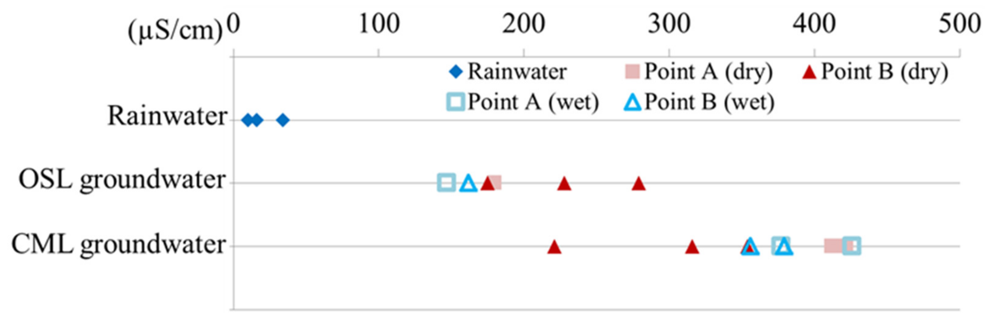
3.4. Electrical Conductivity

Figure 8 shows the EC values of water samples. Rainwater EC (ranging from 9 to 34 μS cm⁻¹) was significantly lower than the values of other samples based on the two-tailed t-test (p < 0.05). Two water samples from the OSLs at Point A showed EC of 147 and 180 μS cm⁻¹. The EC of OSL groundwater at Point B ranged from 162 to 279 μS cm⁻¹; this overlapped the values of CML groundwater. Greater variation in groundwater EC in the CML was observed at Point B than at Point A (from 221 to 379 μS cm⁻¹ and from 377 to 426 μS cm⁻¹, respectively). Overall, the OSL groundwater had significantly lower values than the CML groundwater (p < 0.05). Figure 8 also shows that the EC values of OSL groundwater tended to be higher during dry periods than during wet periods. No such tendency was recognized for CML groundwater.

4. Discussion

4.1. Sources of Groundwater

While semi-perennial to perennial groundwater zones were present in both OSLs and CMLs within the unchanneled hollow, their fluctuation characteristics differed. The responses of CML groundwater to rainfall were small and gentle (Figure 6), presumably because of the hydraulic properties of CMLs, which have low permeability even under saturated conditions and contain small numbers of large pores (Figure 4). Additionally, $\psi$ in the CMLs at Point T was consistently high, even during dry periods (Figure 5c), because the large number of small pores in the CMLs prevents drainage of water stored in the pores during dry periods. In contrast, the OSL groundwater level in the hollow and $\psi$ at Point T showed rapid fluctuations in response to rainfall (Figure 5b and Figure 6). These fluctuations during wet periods suggest rapid rainwater infiltration into and drainage from large pores, reflecting the hydraulic properties of OSLs (Figure 4). The process of groundwater generation in OSLs in the hollow during wet periods can be explained by the conventional conceptual model described in the Introduction section: rainwater vertically infiltrates into the highly permeable OSLs until it reaches the less permeable CMLs. Water then laterally flows along the CML surface, forming a groundwater zone above CMLs in the downslope area. The EC of OSL groundwater tended to be lower during wet periods than during dry periods (Figure 8), suggesting that the infiltration of rainwater with low EC (Figure 8) affected the OSL groundwater during wet periods.

Surprisingly, the groundwater zone remained present for a long period of time in the OSLs in the hollow during dry periods (Figure 6). The high permeability of the OSLs does not allow groundwater in the OSLs to be maintained consistently during dry periods. Additionally, because the study catchment is small, with gentle hillslopes and thin OSLs, no large depression or convergent topography is available to provide water storage. The EC values of OSL groundwater collected from a depth of several tens of centimeters during dry periods were high (175 to 279 μS cm⁻¹; Figure 8). In Japan, reported EC values in soil layers at a few centimeters directly below leaf litter were high (>300 μS cm⁻¹), especially in autumn when many broadleaf trees drop their leaves; these values decreased with infiltration into OSLs [34,35]. Sakuma and Sato [34] showed that the EC values of water collected from OSLs overlying pyroclastic fall deposits in Hokkaido, Japan, were in the range of approximately 30–70 μS cm⁻¹. Miyata et al. [36] reported that, in OSLs at the depth of 20 cm in a granitic catchment in Gifu Prefecture, Japan, the mean EC value of stored water was 17.36 μS cm⁻¹. In a catchment consisting of volcanic rock and sedimentary rock in Akita, Japan, the EC of water stored at approximately 20–40-cm depth in an OSL was 51 μS cm⁻¹ [35]. Compared with the EC values measured in these previous studies, the OSL groundwater EC values observed in the present study during dry periods were surprisingly high. This comparison suggests that the high values of OSL groundwater EC during dry periods are influenced by CML groundwater, which has high EC values (Figure 8); moreover, CML groundwater is an important source of groundwater present in the OSLs during dry periods.

One possible explanation for the contribution of CML groundwater to the groundwater zone in the OSLs involves runoff of CML groundwater into the OSLs via macropores or pipes within the CMLs. However, no such structures were observed in the study catchment. The results of temperature observations (Figure 7) suggested that such runoff of CML groundwater into the OSLs was unlikely; the groundwater temperature in the CMLs showed moderate seasonal variations and minimal impact from diurnal air or rainwater temperature, whereas water in the OSLs was sensitive to air and rainwater temperature. If macropores or pipes had contributed to water flow, the CML groundwater temperature would be affected by air or rainwater temperature, such that it would show sensitive fluctuation during wet periods; during dry periods, the OSL groundwater temperature would show moderate fluctuations driven by runoff of CML groundwater. The EC values of CML groundwater showed no clear difference between dry and wet periods (Figure 8), which is consistent with these inferences.

These findings suggest that CML groundwater contributed to maintenance of the groundwater zone in OSLs in the hollow during dry periods through a mechanism that did not involve runoff of CML groundwater into the OSLs via macropores or pipes.

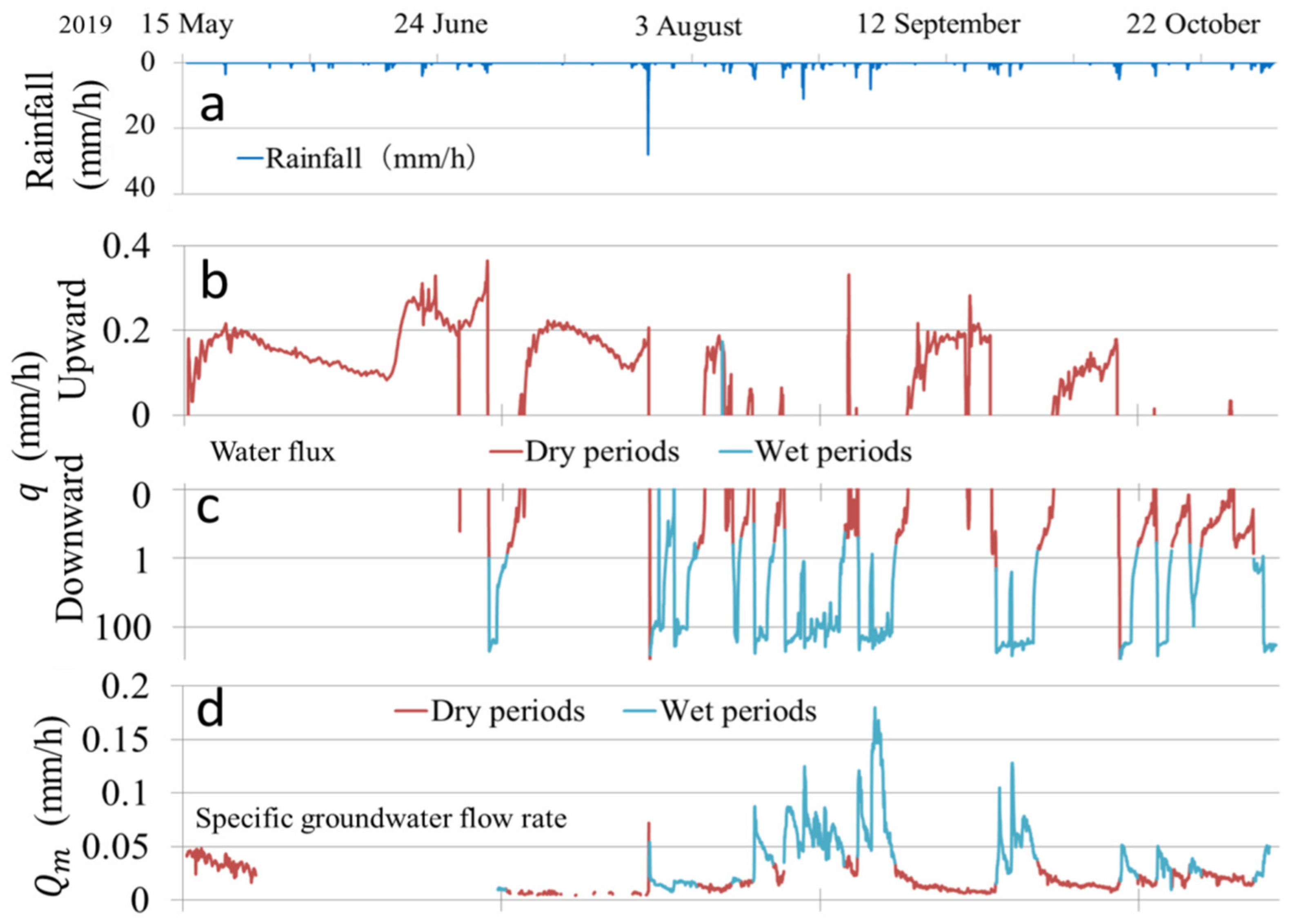
4.2. Water Flow Direction and Flux Analysis across OSL-CML Boundary

4.2.1. Flow Direction Analysis

To examine the contribution of CML groundwater to the OSL groundwater zone in the hollow during dry periods, we analyzed the water flow direction between OSLs and CMLs using the $\psi$ values recorded at Point T. We focused on the flow direction between the 30 and 50 cm tensiometers, which were located immediately above and below the OSL–CML boundary (depth: 31 cm). Figure 9 shows the temporal variations in the difference in total head, $H$, defined as the sum of $\psi$ and the elevation head, between 30 and 50 cm. We used the ground surface as the reference level for calculating elevation head. A positive value of $H$ indicates upward flow from the CMLs into the OSLs, whereas a negative value indicates downward flow from the OSLs into the CMLs. Figure 9 demonstrates that the main flow direction during wet periods was downward.

Figure 10 shows the relationship between simultaneous $\psi$ measurements from the 30 and 50 cm tensiometers (${\psi }_{30}$ and ${\psi }_{50}$, respectively); in this plot, two groups are distinguished according to the flow direction (upward or downward). During wet periods, downward flow was observed for 1104 h, whereas upward flow was observed for only 1 h. Thus, downward flow from the OSLs to the CMLs occurred mainly during wet periods including rainfall periods, indicating that a portion of the rainwater infiltrated into the CMLs and recharged the CML groundwater. Conversely, after the cessation of rainfall, downward flow decreased and the flow direction switched from downward to upward; upward flow was observed during dry periods (Figure 9). Upward and downward flows were observed during a dry period at 2296 and 662 h, respectively (Figure 10). Thus, upward flow consistently occurred during dry periods. The OSLs, with high permeability under saturated conditions and a large number of large pores, became unsaturated and dried up during dry periods. The CMLs, with low permeability under saturated conditions and no large pores, remained nearly saturated even during dry periods. The frequent and long-term occurrence of upward flow can be attributed to these differences in hydraulic properties between OSLs and CMLs.

4.2.2. Upward Flux Analysis during Dry Periods

Next, we analyzed the vertical water flux across the OSL–CML boundary at Point T using $H$. According to Darcy’s Law, water flux, $q$, at the boundary can be calculated as follows:

$$q=-K_{bo}\left({\psi }_{31}\right)\frac{H}{s}$$

(4)

where $K_{bo}$ is the hydraulic conductivity of the OSL–CML boundary, ${\psi }_{31}$ is $\psi$ at the boundary (at 31 cm depth), and $s$ is the distance in the direction of flow (20 cm). We computed ${\psi }_{31}$ as follows:

$${\psi }_{31}=\frac{{\psi }_{50}{s}_{30}+{\psi }_{30}{s}_{50}}{s}$$

(5)

where $s_{30}$ and $s_{50}$ are the vertical distances from the boundary to the 30 and 50 cm tensiometers (i.e., 1 and 19 cm), respectively. $K_{bo}\left({\psi }_{31}\right)$ was calculated using the hydraulic conductivity curve of the OSL–CML boundary shown in Figure 4b.

Figure 11b, c shows the temporal variations in upward and downward $q$, respectively. Note that downward $q$ in Figure 11c is plotted on a logarithmic scale. The maximum upward flux during dry periods was 0.36 mm h⁻¹, observed on 1 July at 17:00, which was extremely small compared to the maximum downward flux during wet periods of 983 mm h⁻¹, which was observed on 9 October at 0:00. However, the upward flux during dry periods averaged 0.16 mm h⁻¹ and totaled 360 mm, equivalent to three-quarters of the total precipitation (468.5 mm). This similarity suggests that the accumulation of water that moved upward from the CMLs into the OSLs in areas where the OSLs were dry ($\psi$ < −10 cm; Figure 10) contributed to the maintenance of the groundwater zone in the OSLs along the hollow (including Points A and B) during dry periods.

To determine whether the calculated upward $q$ can explain the observed groundwater level in the OSLs in the hollow during dry periods, we conducted a crude calculation of the specific groundwater flow rate in the OSLs at the midpoint between Points A and B. The rate of specific groundwater flow in the OSLs at the midway point, $Q_m$, can be approximated as follows:

$$Q_m=\frac{q_m A_C}{A_m}$$

(6)

where $q_m$ is groundwater flux at the midway point, $A_C$ is the cross-sectional area of the groundwater zone at the midway point calculated assuming a triangular area, and $A_m$ is the catchment area at the midway point (0.056 ha). By applying Darcy’s law to saturated groundwater flow in the OSLs between Points A and B, $q_m$ can be approximated as follows:

$$q_m=K_{s\_OSLs}\frac{H_{AB}}{S_s}$$

(7)

where $K_{s\_OSLs}$ is the mean saturated hydraulic conductivity of OSLs (3.38 × 10⁻² cm s⁻¹), $H_{AB}$ is the difference in elevation of the groundwater table in the OSLs between Points A and B, and $S_s$ is the slope length from Points A to B (19.0 m).

Figure 11d shows the temporal variations of $Q_m$ (data are missing from 26 May at 13:00 though 3 July at 10:00 due to the lack of the groundwater level data at Point A). The maximum $Q_m$ was 0.18 mm h⁻¹, observed on 31 August at 14:00 during a wet period. During dry periods, $Q_m$ reached its maximum (0.072 mm h⁻¹) on 27 July at 3:00 and averaged 0.018 mm h⁻¹. The findings in Figure 11b,d indicate that upward $q$ was larger than $Q_m$ for nearly the entire observation period when upward flux was generated. The sums of upward $q$ and $Q_m$ during dry periods with upward flux from 1 July to 31 October were 172.5 and 9.76 mm, respectively. Kondo et al. [37] estimated that mean transpiration in July through October in this region (including the study catchment) was 172 mm. Comparison of these values suggests that most of the upward $q$ is consumed by transpiration (some water that flowed only through the OSLs was presumably also consumed by transpiration), whereas the remaining $q$ could generate the observed saturated groundwater flow in the OSL in the hollow. Thus, water supplied from the CMLs to OSLs as upward flux accumulated and contributed to the groundwater zone in the OSLs in the hollow during dry periods.

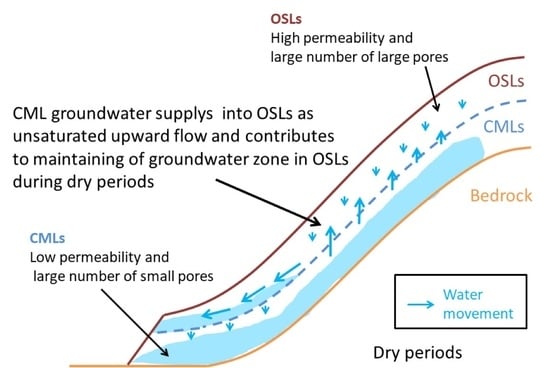
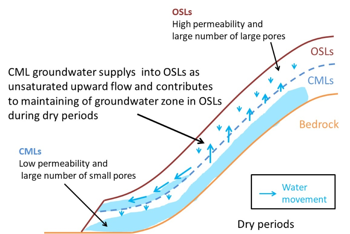
4.3. Conceptual Model of Formation Process of OSL Groundwater Zone

Based on the discussion above, Figure 12 illustrates the formation processes of the groundwater zone in the OSLs in the hollow of the study catchment. During wet periods including rainfall periods (Figure 12a), rainwater vertically infiltrates into the highly permeable OSLs until it reaches the less permeable CMLs; it then becomes perched groundwater above the OSL–CML boundary. The perched groundwater flows downslope along the OSL–CML boundary as saturated lateral flow, thereby expanding or increasing the depth of the groundwater zone in the OSLs in the hollow. In areas where the OSLs are wet ($\psi$ > −10 cm), a portion of this water infiltrates into the CMLs as downward flux (Figure 10) and slowly recharges the CML groundwater.

In contrast, during dry periods (Figure 12b), the contribution of rainwater to the OSL groundwater zone decreases and upward flow from the CMLs occurs mainly in areas where the OSLs are dry ($\psi$ < −10 cm) (Figure 10). This water then flows downslope along the OSL–CML boundary as unsaturated or saturated lateral flow, forming the groundwater zone in the OSLs in the hollow of the downslope area.

4.4. Importance of Water Supply from CMLs to OSLs as Upward Flux during Dry Periods

Upward flux in a headwater catchment has been reported previously [20,38,39], and two mechanisms of upward flux generation have been proposed. One mechanism is unsaturated upward flux resulting from the balance of the matrix potential of soil layers (i.e., unsaturated matrix flow), as observed in this study, which occurs as soil layers become dry and the groundwater level decreases [39,40,41,42]. The other mechanism is saturated upward flux, which occurs in association with the local exfiltration of bedrock groundwater into soil layers through fissures and cracks in the bedrock [20,38,43,44,45]. Although saturated upward flux is often considered as an important water supply process for soil layers, unsaturated upward flux caused by matrix flow has attracted minimal attention because of the small fluxes involved relative to saturated upward fluxes. Frisbee et al. [15] reported large-volume groundwater storage in a depression located near the base of the slope in a 0.60 ha catchment during periods of low water table position. In this case, the soil thickness of the depression was as much as approximately 4 m. From the results of this study, unsaturated upward flux may be an important process that sustains wet soil layers during dry periods in still smaller headwater catchments with thinner soil layers and without saturated upward flux from bedrock.

At Point T in the study catchment, upward flux from the CMLs to the OSLs generally occurred as unsaturated flow during dry periods. Although the maximum upward flux was small (0.36 mm h⁻¹), the total upward flux over the entire observation period was large (360 mm). This continuous upward flux contributed to the maintenance of the groundwater zone in the OSLs in the hollow of the downslope area during dry periods, which presumably caused subsequent volumetric and chemical changes in streamflow. Moreover, in a serpentinite catchment in Hokkaido, Japan, Aipassa [46] described the occurrence of surface slides (a type of slope failure) with the slip surface located at the OSL–CML boundary; such slides were reported to occur on steep slopes when rainfall is sufficiently heavy to saturate the slip surface. Although no traces of such slides were found in the study catchment, presumably because of the low gradient, continuous unsaturated upward flux can influence such slides by raising the groundwater level or expanding the groundwater zone in the OSLs of hollows during rainfall periods through the generation of a small groundwater zone before the rainfall, which reduces the stability of the OSLs. Thus, the present findings emphasize the important role of water supply from CMLs to OSLs during dry periods in the formation of a groundwater zone in OSLs in hollows, in addition to its effects on streamflow and shallow landslides.

5. Conclusions

Detailed hydrological, hydrochemical, and thermal observations in a forested serpentinite headwater catchment containing mineral soil layers composed of thick clayey materials produced by weathering of bedrock (i.e., CMLs), along with hydraulic property measurements in the laboratory, were conducted to elucidate the formation process of the semi-perennial to perennial groundwater zone observed in thin OSLs within an unchanneled hollow in the study catchment, even during dry periods. The groundwater temperature and chemistry suggested that runoff of the CML groundwater into the OSLs via macropores or pipes is unlikely. Instead, water flux analysis across the OSL–CML boundary revealed that unsaturated upward flow from the CMLs into OSLs occurs in areas where the OSLs are dry (pressure head < −10 cm). Accumulation of this upward flux can explain the groundwater zone observed in the OSLs of the hollow during dry periods. We conclude that water infiltrates from the OSLs into CMLs during wet periods (including rainfall periods) and then is supplied into the OSLs as upward flux during dry periods; this upward flux contributes to the generation of a semi-perennial to perennial groundwater zone in the OSLs in the hollow. Land users and management organizations of catchments underlain by thick CMLs should pay attention to volumetric and chemical changes in streamflow and the surface slides that could be caused by the semi-perennial to perennial groundwater zone. In future research, detailed observations of other serpentinite catchments and catchments underlain by other bedrock types with thick CMLs (e.g., mudstone and slate catchments) are needed to determine the generalizability of the present findings.

References

1. Katsuyama, M.; Ohte, N. Determining the sources of stormflow from the fluorescence properties of dissolved organic carbon in a forested headwater catchment. J. Hydrol. 2002, 268, 192–202. [Google Scholar] [CrossRef]
2. Detty, J.M.; McGuire, K.J. Threshold changes in storm runoff generation at a till-mantled headwater catchment. Water Resour. Res. 2010, 46, W07525. [Google Scholar] [CrossRef] [Green Version]
3. Martínez-Carreras, N.; Hissler, C.; Gourdol, L.; Klaus, J.; Juilleret, J. Storage controls on the generation of double peak hydrographs in a forested headwater catchment. J. Hydrol. 2016, 543, 255–269. [Google Scholar] [CrossRef]
4. Bishop, K.; Seibert, J.; Köhler, S.; Laudon, H. Resolving the double paradox of rapidly mobilized old water with highly variable responses in runoff chemistry. Hydrol. Process. 2004, 18, 185–189. [Google Scholar] [CrossRef]
5. Gannon, J.P.; Bailey, S.W.; Mcguire, K.J.; Shanley, J.B. Flushing of distal hillslopes as an alternative source of stream dissolved organic carbon in a headwater catchment. Water Resour. Res. 2015, 51, 8114–8128. [Google Scholar] [CrossRef] [Green Version]
6. Van Asch, T.; Buma, T.; VanBreek, L. A view on some hydrological triggering systems in landslides. Geomorphology 2005, 30, 25–32. [Google Scholar] [CrossRef]
7. Sidle, R.C.; Bogaard, T.A. Dynamic earth system and ecological controls of rainfall-initiated landslides. Earth-Sci. Rev. 2016, 159, 275–291. [Google Scholar] [CrossRef]
8. Mosley, M.P. Streamflow generation in a forested watershed, New Zealand. Water Resour. Res. 1979, 15, 795–806. [Google Scholar] [CrossRef]
9. Mosley, M.P. Subsurface flow velocities through selected forest soils South Island, New Zealand. J. Hydrol. 1982, 55, 65–92. [Google Scholar] [CrossRef]
10. Pearce, A.J.; Stewart, M.K.; Sklash, M.G. Storm runoff generation in humid headwater catchments. 1. Where does the water come from? Water Resour. Res. 1986, 22, 1263–1272. [Google Scholar] [CrossRef]
11. McGlynn, B.L.; McDonnell, J.J.; Brammer, D.D. A review of the evolving perceptual model of hillslope flowpaths at the Maimai catchments, New Zealand. J. Hydrol. 2002, 257, 1–26. [Google Scholar] [CrossRef]
12. Wilson, G.V.; Jardine, P.M.; Luxmoore, R.J.; Zelazny, L.W.; Todd, D.E.; Lietzke, D.A. Hydrogeochemical processes controlling subsurface transport from an upper subcatchment of walker branch watershed during storm events. 2. Solute transport processes. J. Hydrol. 1991, 123, 317–336. [Google Scholar] [CrossRef]
13. Soulsby, C. Hydrological controls on acid runoff generation in an afforested headwater catchment at Llyn Brianne, Mid-Wales. J. Hydrol. 1992, 138, 431–448. [Google Scholar] [CrossRef]
14. Sidle, R.C.; Tsuboyama, T.; Noguchi, S.; Hosoda, I.; Fujieda, M.; Shimizu, T. Stormflow generation in steep forested headwaters: A linked hydrogeomorphic paradigm. Hydrol. Process. 2000, 14, 369–385. [Google Scholar] [CrossRef]
15. Frisbee, M.D.; Allan, C.J.; Thomasson, M.J.; Mackereth, R. Hillslope hydrology and wetland response of two small zero-order boreal catchments on the Precambrian Shield. Hydrol. Process. 2007, 21, 2979–2997. [Google Scholar] [CrossRef]
16. Fujimoto, M.; Ohte, N.; Tani, M. Effects of hillslope topography on hydrological responses in a weathered granite mountain, Japan: Comparison of the runoff response between the valley-head and the side slope. Hydrol. Process. 2008, 22, 2581–2594. [Google Scholar] [CrossRef]
17. Uhlenbrook, S.; Frey, M.; Leibundgut, C.; Maloszewski, P. Hydrograph separations in a mesoscale mountainous basin at event and seasonal timescales. Water Resour. Res. 2002, 38, 1096. [Google Scholar] [CrossRef] [Green Version]
18. Gabrielli, C.P.; McDonnell, J.J.; Jarvis, W.T. The role of bedrock groundwater in rainfall-runoff response at hillslope and catchment scales. J. Hydrol. 2012, 450–451, 117–133. [Google Scholar] [CrossRef]
19. Zhao, S.; Hu, H.; Harman, C.J.; Tian, F.; Tie, Q.; Liu, Y.; Peng, Z. Understanding of storm runoff generation in a weathered, fractured granitoid headwater catchment in northern China. Water 2019, 11, 123. [Google Scholar] [CrossRef] [Green Version]
20. Uchida, T.; Asano, Y.; Ohte, N.; Mizuyama, T. Analysis of flowpath dynamics in a steep unchannelled hollow in the Tanakami Mountains of Japan. Hydrol. Process. 2003, 17, 417–430. [Google Scholar] [CrossRef]
21. Katsura, S.; Kosugi, K.; Mizutani, T.; Okumura, S.; Mizuyama, T. Effects of bedrock groundwater on spatial and temporal variations in soil mantle groundwater in a steep granitic headwater catchment. Water Resour. Res. 2008, 44, W09430. [Google Scholar] [CrossRef] [Green Version]
22. Hiura, T.; Uejima, N.; Okuda, A.; Hojo, H.; Ishida, T.; Okuyama, S. Crowding effects on diameter growth for Abies sachalinensis, Quercus crispula and Acer mono trees in a northern mixed forest, Nakagawa Experimental Forest. Res. Bull. Hokkaido Univ. For. 1998, 55, 255–261, (In Japanese with English Summary). [Google Scholar]
23. Kobayashi, M.; Templer, P.H.; Katayama, A.; Seki, O.; Takagi, K. Early snowmelt by an extreme warming event affects understory more than overstory trees in Japanese temperate forest. Ecosphere 2022, 13, e4182. [Google Scholar]
24. Hiura, T.; Sato, G.; Hayashi, I. Long-term forest dynamics in response to climate change in northern mixed forests in Japan: A 38-year individual-based approach. For. Ecol. Manag. 2019, 449, 117469. [Google Scholar] [CrossRef]
25. Hiura, T.; Fujiwara, K. Density-dependence and co-existence of conifer and broad-leaved trees in a Japanese northern mixed forest. J. Veg. Sci. 1999, 10, 843–850. [Google Scholar] [CrossRef]
26. Suzuki, T. Formative processes of specific features of serpentinite mountains. Trans. Jpn. Geomorphol. Union 2006, 27, 417–460. [Google Scholar]
27. Nakata, N.; Kojima, S. Effects of serpentine substrate on vegetation and soil development with special reference to Picea glehnii forest in Teshio District, Hokkaido, Japan. For. Ecol. Manag. 1987, 20, 265–290. [Google Scholar] [CrossRef]
28. Tani, M. Runoff generation processes estimated from hydrological observations on a steep forested hillslope with a thin soil layer. J. Hydrol. 1997, 200, 84–109. [Google Scholar] [CrossRef]
29. Newman, B.D.; Campbell, A.R.; Wilcox, B.P. Lateral subsurface flow pathways in a semiarid ponderosa pine hillslope. Water Resour. Res. 1998, 34, 3485–3496. [Google Scholar] [CrossRef]
30. Gabbrielli, R.; Pandolfini, T.; Vergnano, O.; Palandri, M.R. Comparison of two serpentine species with different nickel tolerance strategies. Plant Soil 1990, 122, 271–277. [Google Scholar] [CrossRef]
31. Kosugi, K. Lognormal distribution model for unsaturated soil hydraulic properties. Water Resour. Res. 1996, 32, 2697–2703. [Google Scholar] [CrossRef]
32. Mualem, Y. A new model for predicting the hydraulic conductivity of unsaturated porous media. Water Resour. Res. 1976, 12, 513–522. [Google Scholar] [CrossRef] [Green Version]
33. Ishii, Y.; Kodama, Y.; Nakamura, R.; Ishikawa, N. Water balance of a snowy watershed in Hokkaido, Japan. In Northern Research Basins Water Balance (Proceedings of a Workshop Held at Victoria, Canada, March 2004); IAHS Publication: Oxfordshire, UK, 2004; Volume 290, pp. 13–27. [Google Scholar]
34. Sakuma, T.; Satoh, F. Dynamics of inorganic elements in soils under deciduous forest (Part 1). Res. Bull. Coll. Exp. For. 1978, 44, 537–552, (In Japanese with English Summary). [Google Scholar]
35. Hayakawa, A.; Ota, H.; Asano, R.; Murano, H.; Ishikawa, Y.; Takahashi, T. Sulfur-based denitrification in streambank subsoils in a headwater catchment underlain by marine sedimentary rock in Akita, Japan. Front. Environ. Sci. 2021, 9, 664488. [Google Scholar] [CrossRef]
36. Miyata, S.; Uchida, T.; Asano, Y.; Ando, H.; Mizuyama, T. Effects of bedrock groundwater seepage on runoff generation at a granitic first order stream. J. Jpn. Soc. Eros. Control. Eng. 2003, 56, 13–19, (In Japanese with English Abstract). [Google Scholar]
37. Kondo, J.; Nakazono, M.; Watanabe, T.; Kuwagata, T. Hydrological climate in Japan (3) Evapotranspiration from forest. J. Jpn. Soc. Hydrol. Water Resour. 1992, 5, 8–18. [Google Scholar] [CrossRef]
38. McGlynn, B.L.; McDonnell, J.J.; Shanley, J.B.; Kendall, C. Riparian zone flowpath dynamics during snowmelt in a small headwater catchment. J. Hydrol. 1999, 222, 75–92. [Google Scholar] [CrossRef]
39. Harria, A.H.; Shand, P. Near-stream soil water-groundwater coupling in the headwaters of the Afon Hafren, Wales: Implications for surface water quality. J. Hydrol. 2006, 331, 567–579. [Google Scholar] [CrossRef]
40. Tsujimura, M. Behavior of subsurface water in a steep forested slope covered with a thick soil layer. J. Jpn. Assoc. Hydrol. Sci. 1993, 23, 3–18, (In Japanese with English Abstract). [Google Scholar]
41. Tsurita, T.; Yoshinaga, S.; Abe, T. Estimation of vertical water flux through forest subsoil using Buckingham-Darcy Equation. J. Jpn. For. Soc. 2009, 91, 151–158, (In Japanese with English Abstract). [Google Scholar] [CrossRef] [Green Version]
42. Gannon, J.P.; McGuire, K.J.; Bailey, S.W.; Bourgault, R.R.; Ross, D.S. Lateral water flux in the unsaturated zone: A mechanism for the formation of spatial soil heterogeneity in a headwater catchment. Hydrol. Process. 2016, 31, 3568–3579. [Google Scholar] [CrossRef] [Green Version]
43. Montgomery, D.R.; Dietrich, W.E.; Torres, R.; Anderson, S.P.; Heffner, J.T.; Loague, K. Hydrologic response of a steep, unchanneled valley to natural and applied rainfall. Water Resour. Res. 1997, 33, 91–109. [Google Scholar] [CrossRef]
44. Haga, H.; Matsumoto, Y.; Matsutani, J.; Fujita, M.; Nishida, K.; Sakamoto, Y. Flow paths, rainfall properties, and antecedent soil moisture controlling lags to peak discharge in a granitic unchanneled catchment. Water Resour. Res. 2005, 41, W12410. [Google Scholar] [CrossRef]
45. Masaoka, N.; Kosugi, K.; Yamakawa, Y.; Tsutsumi, D. Processes of bedrock groundwater seepage and their effects on soil water fluxes in a foot slope area. J. Hydrol. 2016, 535, 160–172. [Google Scholar] [CrossRef]
46. Aipassa, M.I. Landslide debris movement and its effects on slope and river channel in mountainous watershed. Res. Bull. Coll. Exp. For. 1991, 48, 375–418. [Google Scholar]
Figure 1. Maps of (a) Hokkaido, (b) the Kunneshiri Mountain area in Nakagawa Experimental Forest, and (c) the study catchment. In panel (b), black and gray contours represent intervals of 10 and 2 m, respectively. In panel (c), the contour interval is 1 m. Dotted and dashed lines in panel (c) indicate an unchanneled hollow in the study catchment and the catchment boundary, respectively.
Water 14 03122 g001
Figure 2. Flowchart of methodology of this study.
Water 14 03122 g002
Figure 3. Photograph of the trench at Point S. White dotted lines indicate boundaries between the OSLs and CMLs and between the CMLs and bedrock. Solid red circles indicate the depths at which undisturbed core samples were collected.
Water 14 03122 g003
Figure 4. (a) Water retention curves and (b) hydraulic conductivity curves of the OSLs, CMLs, and boundary zone between the OSLs and CMLs.
Water 14 03122 g004
Figure 5. (a) Rainfall and ψ in the (b) OSLs (30 cm) and (c) CMLs (50 and 80 cm). Dashed line in panel (b) represents ψ = −10 cm.
Water 14 03122 g005
Figure 6. (a) Rainfall and groundwater levels at (b) Point A and (c) Point B. The groundwater level is presented as depth below the ground surface. Dashed lines in panels (b,c) indicate the boundary between the OSLs and CMLs.
Water 14 03122 g006
Figure 7. (a) Rainfall and air temperature and groundwater temperature at (b) Point A and (c) Point B.
Water 14 03122 g007
Figure 8. EC of collected water samples.
Water 14 03122 g008
Figure 9. (a) Rainfall and (b) the difference in total head between the depths of 30 and 50 cm at Point T.
Water 14 03122 g009
Figure 10. Relationship between simultaneous ψ 30 and ψ 50 observations. Dashed line represents ψ = −10 cm.
Water 14 03122 g010
Figure 11. (a) Rainfall, (b) upward and (c) downward water flux at Point T, and (d) rate of specific groundwater flow at the midpoint between Points A and B.
Water 14 03122 g011
Figure 12. Formation processes of the groundwater zone within the OSLs in the study catchment during (a) wet periods and (b) dry periods.
Water 14 03122 g012