

Effects of Artificial Water Withdrawal on the Terrestrial Water Cycle in the Yangtze River Basin


1
State Key Laboratory of Simulation and Regulation of Water Cycle in River Basin, China Institute of Water Resources and Hydropower Research, Beijing 100038, China
2
Department of Water Resources, China Institute of Water Resources and Hydropower Research, Beijing 100038, China
*
Author to whom correspondence should be addressed.
Water 2022, 14(19), 3117; https://doi.org/10.3390/w14193117
Submission received: 10 August 2022
/
Revised: 27 September 2022
/
Accepted: 28 September 2022
/
Published: 3 October 2022
(This article belongs to the Special Issue Impacts of Anthropogenic Activities on Watersheds in a Changing Climate Ⅱ)
Abstract
:Clarifying the response of the terrestrial water cycle to the influence of climate change and human activities and accurately grasping the variations in the water cycle and water resources under the changing environment are the scientific basis for achieving the sustainable development of the Yangtze River Economic Belt. In this paper, a dataset of rasterized water consumption in the Yangtze River Basin was constructed, and an artificial water withdrawal module considering the process of water intake, water consumption and drainage was designed, which was coupled with the land surface model CLM4.5. Based on the multi-scale validation in the Yangtze River Basin, two numerical simulation experiments were carried out to reveal the impact of artificial water withdrawal on the water cycle process in the Yangtze River Basin. The results indicate that artificial water withdrawal leads to an 0.1–0.3 m increase in groundwater table depth in most areas of the basin, and agricultural irrigation leads to a 0–0.03 mm3/mm3 increase in soil moisture in most areas. Climate change dominates the variation of discharge in the Yangtze River basin and leads to an increase in discharge at most stations.
1. Introduction
For a long time, the natural water cycle process and the evolution of water resources in the Yangtze River Basin have undergone certain changes due to the influence of various natural and human factors, such as the continuously increasing population pressure, high-intensity development of water and soil resources, and the decreasing stability of the water system under climate change [1]. Frequent water disasters, aggravated water pollution and water shortage in some regions are still prominent, leading to an imbalance between socio-economic development and the carrying capacity of resources and the environment, which has become a major bottleneck restricting the sustainable development of the Yangtze River Basin [2,3]. Therefore, it is of great scientific value and practical significance to analyze the spatio-temporal distribution characteristics of the terrestrial water cycle in the Yangtze River Basin under the influence of climate change and human activities [4] and to reveal the changes and causes of various elements of the water cycle process, which will support the implementation of the national strategy of the protection of the Yangtze River and the green development of the Yangtze River Economic Belt [5].
Models are the main tools to study the impact of climate change and human activities on the water cycle process, and there are usually two types of models, namely the distributed hydrological models and the land surface models. The distributed hydrological model is a mathematical model with a physical mechanism to describe the water cycle process in the basin [6,7]. It can accurately describe the two-dimensional hydrological process and reflect the state and variations of fluxes in the water cycle process [8]. The grid-based land surface model can better reflect the water and energy exchange between the land and atmosphere and the vegetation growth process [9,10,11,12]. However, the traditional hydrological models fail to fully consider the effects of surface radiation, humidity, wind speed and other factors, and they struggle to fully reveal the impact of climate change on the terrestrial water cycle process [13]. Most land surface models have a rough description of the natural-social dualistic water cycle process [14], mainly focus on the variation of water cycle fluxes in the vertical direction, and lack the description of the lateral routing process [15]. Therefore, it can be seen that the current terrestrial water cycle models have huge differences in considering the impact of climate change and human activities on the water cycle process.
To shed light on the effects of human activities on the water cycle process, extensive efforts have been carried out to improve the model. These studies can be roughly divided into two categories. One is to add a natural water cycle process module to the model, while the other is to couple a social water cycle process module in the model. For the former, many researchers have coupled the runoff and routing module of the hydrological model to the land surface model to form a land surface-hydrological model. For instance, Jiao et al. developed the mesoscale eco-hydrological model CLM-GBHM, which realized the simulation of runoff, land surface processes, and vegetation dynamics by coupling CLM4.0 with the distributed hydrological model GBHM. The model was used to carry out several numerical simulation experiments, and the mutual-feedback relationship between vegetation and climate change was revealed [16]. Beoit et al. coupled the land surface model CLASS with the distributed hydrological model WATFLOOD to develop the land surface and hydrological coupling model WATCLASS, which realized the coupling with the mesoscale climate model [17]. For the latter, researchers have coupled modules such as water consumption, which represent social water cycle processes, directly into land surface models to reveal the effects of water intake processes. For example, a water transfer model was developed and coupled with the land surface model BATS by Chen et al. [18]. On this basis, it was further coupled with the regional climate model RegCM3. The influence of water transfer in the middle route of the South-to-North Water Diversion Project on regional climate was carried out by the coupled model. Zou et al. [19] coupled the groundwater exploitation scheme to CLM3.5 and coupled the improved CLM3.5 model to the regional climate model RegCM3 to simulate the impact of water withdrawal on the climate in the Haihe River Basin [20]. The studies mostly focus on the impact of human activities on meteorological elements but less on the impact of human activities on water cycle elements, such as soil moisture and evapotranspiration. Therefore, in this study, an artificial water withdrawal scheme was developed and coupled with the CLM4.5 land surface model in the Yangtze River Basin. On the basis of the multi-scale validation, the impact of artificial water withdrawal on the water cycle process was revealed through two numerical simulation experiments.
2. Materials and Methods
2.1. Study Area
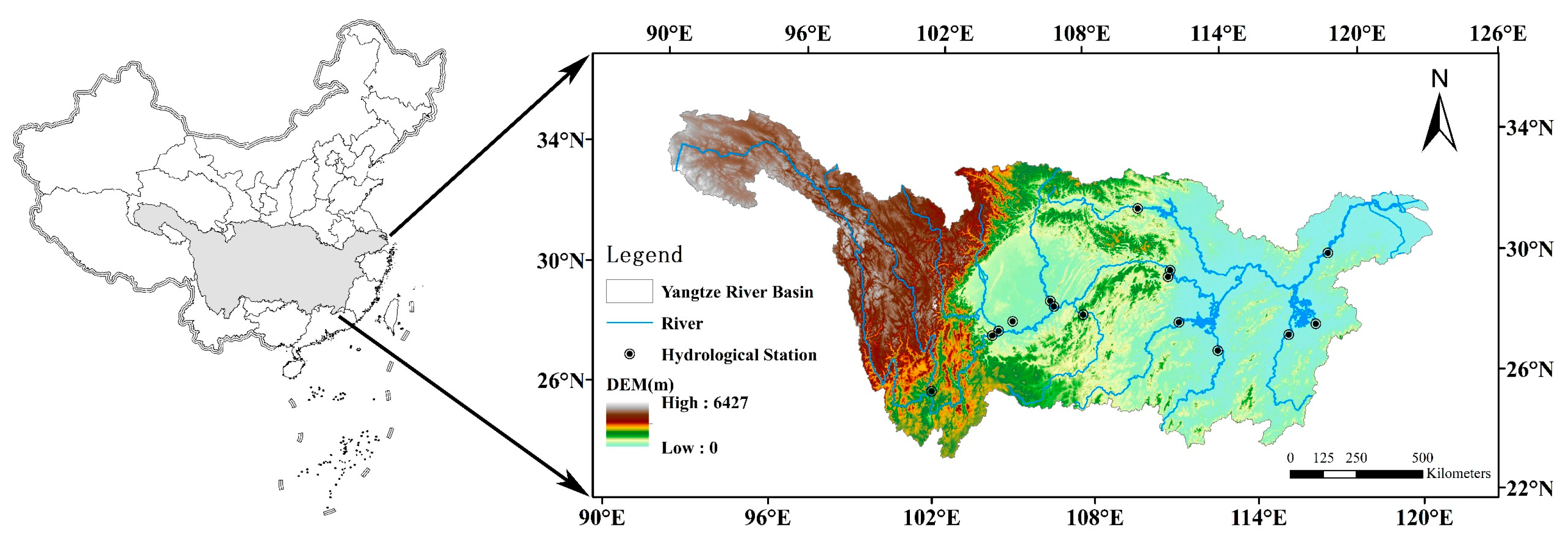
The Yangtze River Basin is located between 90°33′~122°25′ E and 24°30′~35°45′ N, with a mainstream of more than 6300 km in length. Figure 1 shows the topography and river stream of the Yangtze River Basin. The upper reaches of the Yangtze River, from the headwaters to Yichang, are about 4500 km long and control a drainage area of about 1 million km2. The main tributaries of the upper reaches are the Yalong River, the Min River, the Tuo River, the Jialing River and the Wu River. The middle reaches of the Yangtze River, from Yichang to the mouth of Poyang Lake, are about 950 km long and control a drainage area of about 680,000 km2. The main tributaries of the middle reaches are the Qing River, the Han River, the Dongting Lake, and the Poyang Lake. The lower reaches of the Yangtze River, from Hukou to the mouth of the Yangtze River, are about 930 km long and control a drainage area of about 120,000 km2. The main tributaries in the lower reaches are the Qingyi River and the Shuiyang River. There are many types of landforms in the basin, including plateaus, mountains, hills, plains, basins and lakes. The Yangtze River Basin is dominated by mountains and hills, accounting for 40.6% and 30.8%, respectively. The complex geographical environment and topography of the Yangtze River Basin have created different climate types. The climate at the headwaters of the Yangtze River Basin is cold and dry with a plateau climate; other regions are controlled by the cold high pressure of Siberia and Mongolia in winter and the subtropical high pressure in summer, which is a typical subtropical monsoon climate. Except for headwaters, the average annual temperature in other regions is above 12 °C, with a distribution of high temperatures in the southeast and low temperatures in the northwest. The lowest temperature in January is below 0 °C on average, and the highest temperature in July is close to 20 °C on average. Affected by the subtropical monsoon climate, the temporal and spatial distribution of precipitation in the basin is uneven. Spatially, the distribution generally decreases from southeast to northwest; temporally, the precipitation is mainly concentrated from April to October, accounting for about 80% of the annual precipitation [21].
2.2. Data
The data used in this paper include meteorological data, hydrological data, land surface data assimilation products, and socio-economic data. The meteorological data came from the China meteorological forcing dataset (1979–2015) [22] (hereinafter referred to as CMFD). It was used to drive the land surface model with a temporal resolution of 3 h and a horizontal spatial resolution of 0.1 degrees. The dataset was produced by merging a variety of data sources, including China Meteorological Administration station data, TRMM satellite precipitation analysis data, GLDAS data, GEWEX-SRB radiation data, and Princeton forcing data. The dataset included seven elements, near-surface air temperature, near-surface air pressure, near-surface air specific humidity, near-surface wind speed, surface downward shortwave radiation, surface downward longwave radiation, and a precipitation rate. Compared with GLDAS, TRMM and other datasets, CMFD had higher accuracy in mean bias error (MBE), root-mean-square error (RMSE) and coefficient of determination (R2) [23]. The hydrological data came from the Hydrological Yearbook, including the monthly discharge data of 15 hydrological stations. The information is shown in Table 1, and the station distribution is shown in Figure 1.
The Global Land Data Assimilation System (GLDAS-Noah) version 2.0 (NASA, Washington, DC, USA) was used to verify the simulation results of the land surface model. The dataset had a temporal resolution of 1 month and a horizontal spatial resolution of 0.25 degrees, including the fluxes of various elements in the water cycle process, such as soil moisture and evapotranspiration, and energy balance processes, such as sensible heat and latent heat [24].
The socio-economic data came from the China Water Resources Bulletin and China Statistical Yearbook from 1997 to 2015. The China Water Resources Bulletin data included the water consumption for domestic, industrial, agricultural and ecological purposes of cities in the Yangtze River Basin. The China Statistical Yearbook included the irrigated area, population and GDP of cities in the Yangtze River Basin. In order to spatially rasterize the socio-economic data to match the land surface model, the proportion of global irrigated area data with a spatial resolution of 0.1 degrees [25], the population density data with a 1 km resolution in six periods (1980, 1990, 2000, 2005, 2010, 2015) [26] and the GDP data with a 1 km resolution in five periods (1995, 2000, 2005, 2010, 2015) [27] were also collected.
2.3. Methodology
2.3.1. Description of CLM Model
The land surface model CLM4.5 was used to simulate the land surface and hydrological process in the Yangtze River Basin. CLM4.5 was developed by the National Center for Atmospheric Research [28], and it is the land component of the community earth system model (CESM) 1.2.0 [29]. The CLM4.5 is a process-based model which can simultaneously simulate surface energy flux processes, water cycle processes, and biogeochemical cycles. The model takes the grid as the basic computing unit, and a three-level nested subgrid hierarchy is used to represent the spatial surface heterogeneity of grid cells. Each grid is composed of multiple land units, columns and PFTs. A land unit is the first subgrid level to capture the widest spatial patterns of subgrid heterogeneity, including vegetation, lakes, glaciers, cities and crops. The second subgrid level is a column, which is used to characterize the potential variability in the soil and snow state variables within a land unit. It can be divided into up to fifteen layers, including a maximum of five layers of snow and a fixed ten layers of soil. The third subgrid level involves PFTs, which mainly represent the differences in the biophysical and biogeochemical parameters between broad categories of plants. The model is simulated independently at each subgrid level, and each subgrid level has its own diagnostic variables.
The model parameterizes interception, throughfall, canopy drip, snow accumulation and melt, water transfer between snow layers, infiltration, evaporation, surface runoff, sub-surface drainage, redistribution within the soil column, and groundwater discharge and recharge to simulate changes in canopy water, surface water, snow water, soil water, and soil ice, and water in the unconfined aquifer. The total water balance of the system could be expressed as follows:
where is the liquid part of precipitation, is the solid part of precipitation, is ET from vegetation, is ground evaporation, is surface runoff, is runoff from surface water storage, is subsurface drainage, and are liquid and solid runoff from glaciers, wetlands, and lakes, and runoff from other surface types due to snow capping, is the number of soil layers, and is the time step.
2.3.2. Artificial Water Withdrawal Module
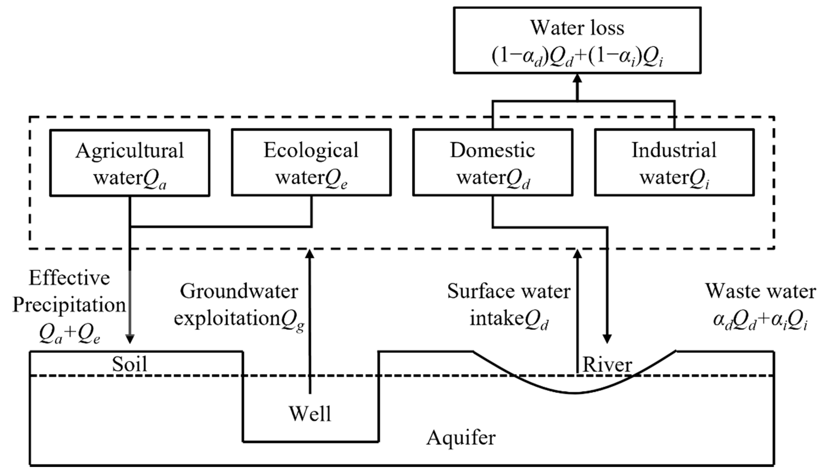
In order to reflect the influence of artificial water intake on the water cycle process, an artificial water withdrawal module was built and coupled with the CLM model [30]. Since land surface simulations are usually oriented to a large scale, and water delivery and other processes in the social water cycle involve complex and elaborate urban pipe networks [31,32,33], only the processes of water intake, water use, and drainage were initially considered in this scheme, which is shown in Figure 2.
We assumed that humans took water from rivers and groundwater wells and that groundwater was directly exploited from the grid cell, while surface water was preferentially taken from the grid cell. If the storage volume of the grid cell cannot meet the requirements, the deficit water would be drawn from adjacent grid cells according to the topology of the river network. The surface water intake can be expressed as follows:
where S and are the surface water amount before and after water withdrawal, respectively, is the surface water intake rate, and is the water intake time.
Groundwater exploitation leads to an increase in the depth of groundwater, so groundwater exploitation can be expressed as follows:
where is the groundwater pumping rate, s is the grid area, and and are the groundwater table depth before and after pumping, respectively. and are the water storage volume of the underground aquifer before and after pumping, respectively.
Water consumption was divided into four categories: agricultural, industrial, domestic and ecological. The total water consumption should satisfy the following equilibrium equation:
where , , , and are the water consumption rates for agricultural, industrial, domestic and ecological water use, respectively. , , and are the proportions of groundwater intaken for agricultural, industrial, domestic and ecological water use, respectively.
In the drainage process, agricultural water and ecological water directly enter the soil surface in the form of effective precipitation after being used and participate in the subsequent natural water cycle process. The process can be expressed as follows:
where and are the rate of water entering the soil before and after agricultural and ecological water withdrawal, respectively.
After the industrial water and domestic water were used, part of the water was dissipated and returned to the atmosphere in the form of evaporation, and the remaining part flowed into the river in the form of wastewater to participate in the subsequent natural water cycle process. The process can be expressed as follows:
where and are the efficiency of domestic and industrial water use, respectively. and are the river flow before and after domestic and industrial water use, respectively. and are the evaporation before and after domestic and industrial water use, respectively.
2.3.3. Experimental Design
In order to reveal the influence of artificial water withdrawal on the water cycle process, two experiments were designed for comparative analysis. The scheme is shown in Table 2. The model used in Experiments 1 and 2 and the simulation period were exactly the same; the only difference was that the model did not consider the artificial water withdrawal in Experiment 1. Therefore, by comparing the results of Experiments 1 and 2, the influence of artificial water withdrawal on various elements of the hydrological process could be revealed. In order to ensure a stable initial state of the model, the meteorological data from 1981 to 1990 was used to drive the model, and the model was simulated 5 times for a total of 50 years to balance the initial condition. The final state was saved as the initial state.
3. Results
3.1. Water Consumption Estimate
Since the spatial resolution of the simulation was 0.1 degrees, the agricultural, industrial and domestic water use data were spatially rasterized according to the following formula.
where , and are the agricultural, industrial and domestic water consumption of each grid cell, respectively. , and are the agricultural, industrial and domestic water consumption of the city where each grid unit is located. area, gdp and pop are the irrigated area, GDP and population of each grid cell, respectively. AREA, GDP and POP are the irrigated area, GDP and population of the city where each grid cell is located. For ecological water consumption, it was assumed that the proportion of each grid cell was equal to the proportion of the city where it was located.
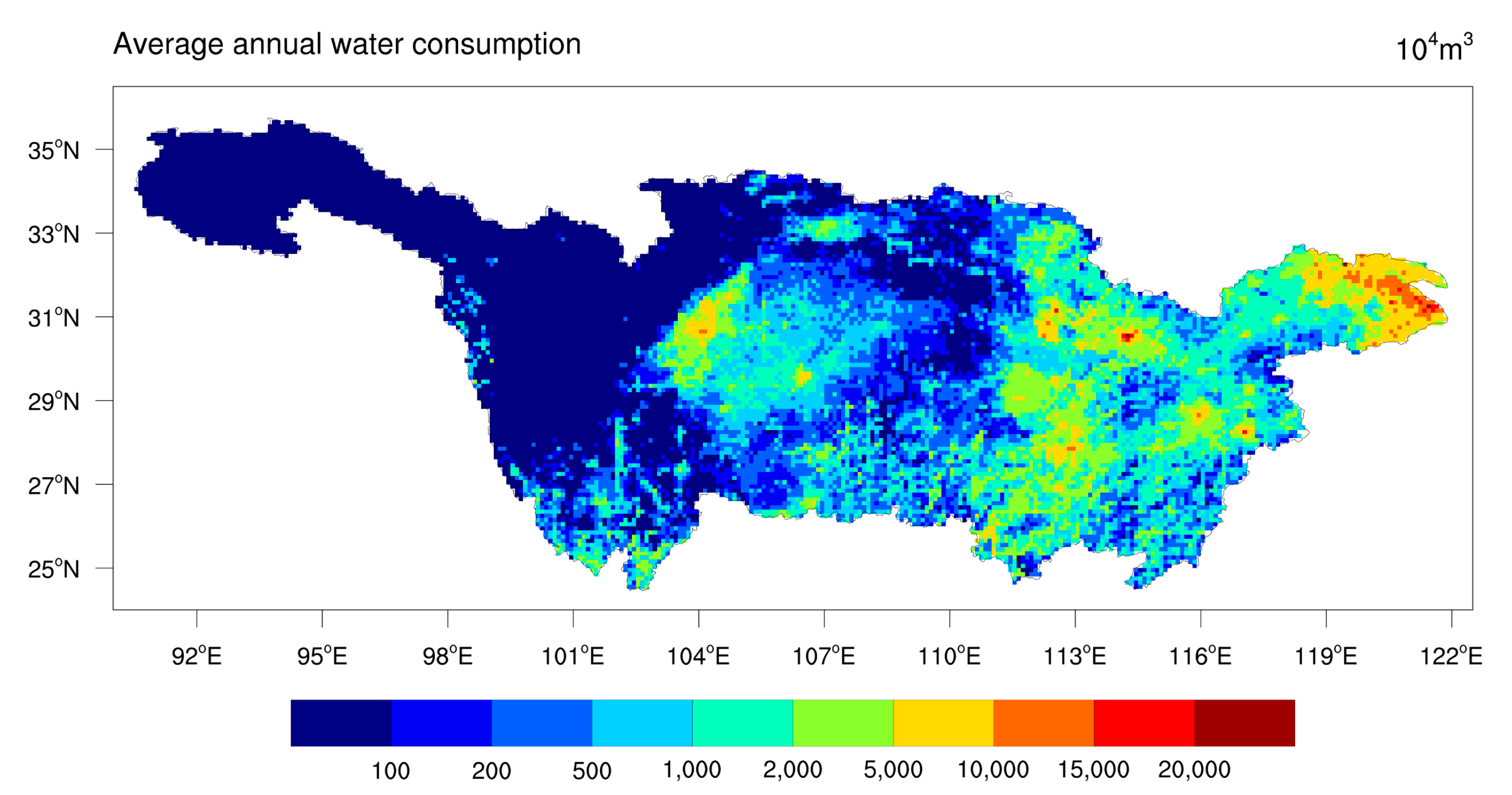
The annual average water consumption in the Yangtze River Basin from 1979 to 2015 is shown in Figure 3. The water consumption was more in the regions with large populations and rapid economic development, such as the Yangtze River Delta urban agglomeration. The water consumption of each grid cell here was more than 10 million m3, and some parts of the Yangtze River Delta could even reach more than 100 million m3. The upper reaches of the Jinsha River Basin were mostly ethnic minority autonomous regions, with vast land, sparsely populated areas, backward industries, and less available arable land, so the total water consumption was very low: the average annual water consumption of each grid cell was less than 1 million m3.
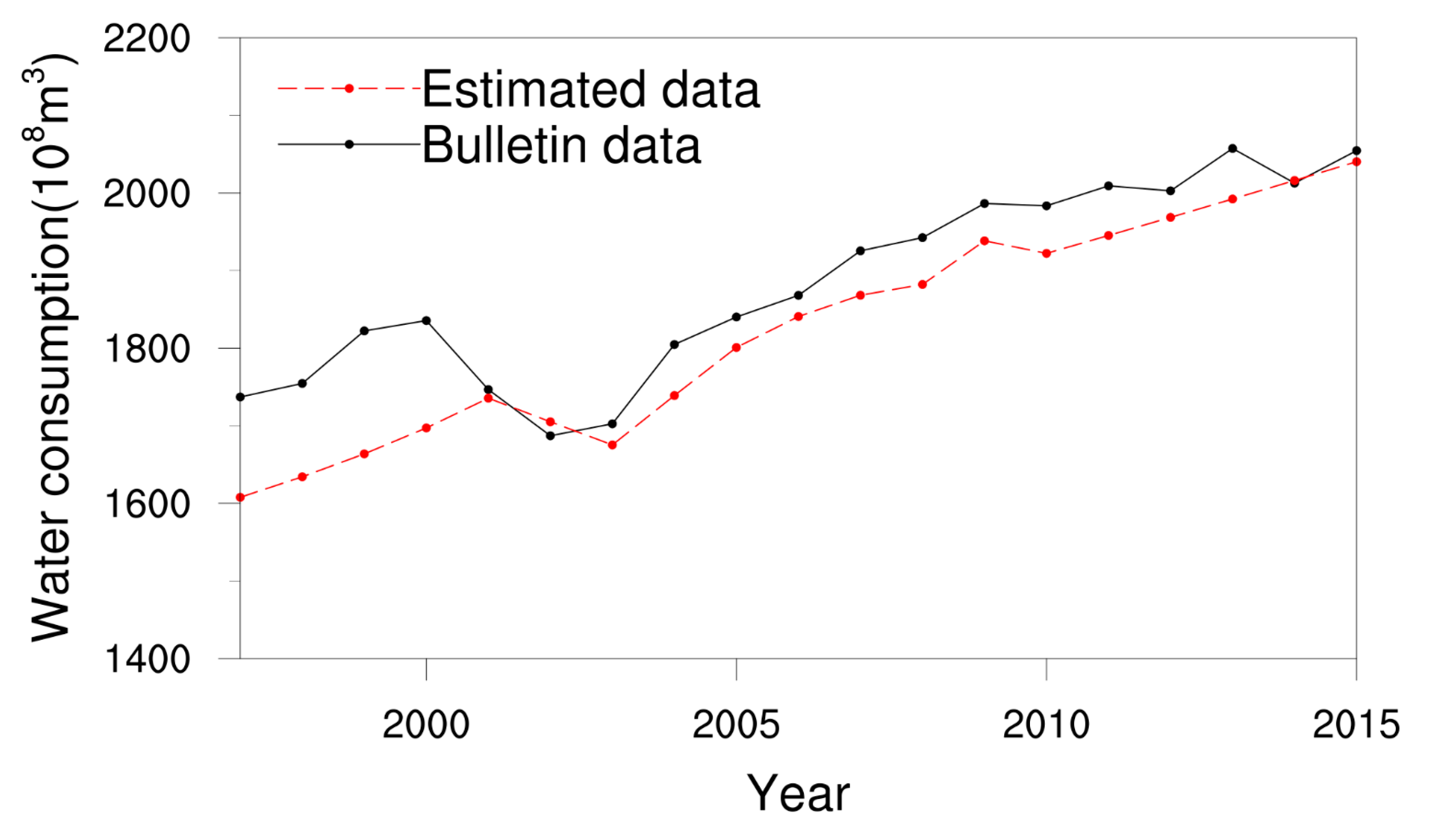
In order to verify the accuracy of the estimated water consumption, the water consumption of each grid cell was accumulated to obtain the total water consumption of the Yangtze River Basin, which was compared with the annual water consumption data from the Yangtze River Basin Water Resources Bulletin since 1997. The results are shown in Figure 4. The variation trend between the two was basically the same, and the error was not more than ±10%. Therefore, the estimated data could be considered accurate. Due to the limited period of data, the water consumption data from 1979 to 1996 were estimated based on the average growth rate of water consumption from 1997 to 2015.
3.2. Model Validation
3.2.1. Discharge Validation
The measured monthly discharge data from 15 hydrological stations were used to validate the discharge processes. The Nash–Sutcliffe efficiency coefficient (NSE) [34] and relative error (PBIAS) [35] were applied to assess the model performance. The NSE reflects the matching degree between the simulated value and the observed value. The closer it is to 1, the better the simulation performance is. The PBIAS reflects the average deviation between the simulated value and the observed value, and the smaller the value, the better the simulation performance. The formulas were expressed as follows:
Where means the observed discharge, means the simulated discharge, means the average observed discharge, and is the number of time steps.
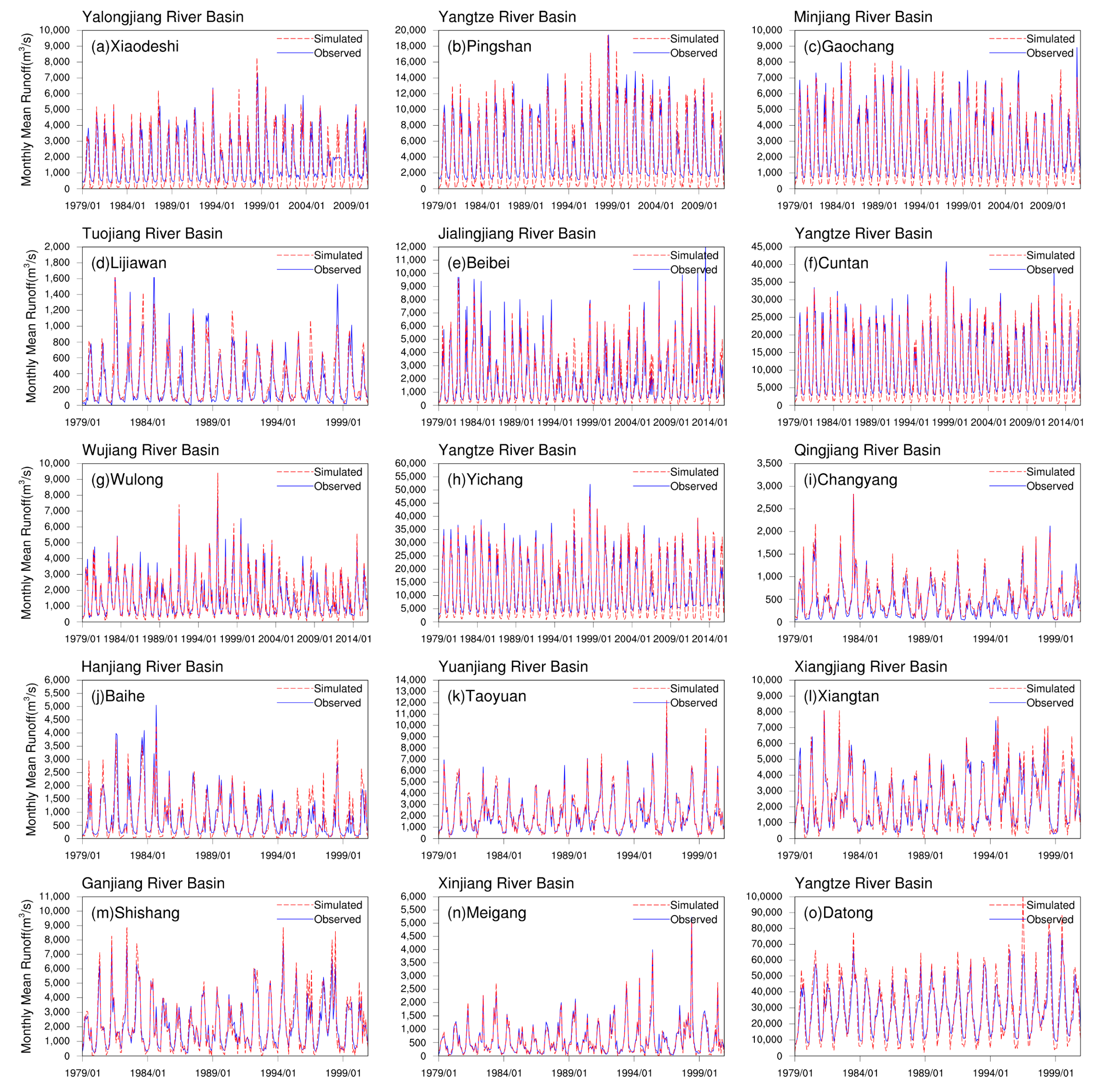
The CLM model can simulate both the water cycle process and the energy balance process, and the description of the internal spatial differences of the grid cells was very detailed, involving a large number of parameters. Table 3 lists the parameters that need to be calibrated, their meanings, and the calibrated values. Figure 5 shows the simulated and observed discharge process of 15 hydrological stations in the main and tributaries of the Yangtze River Basin. Table 4 lists the simulation performance of the model for the monthly discharge process of 15 hydrological stations in the Yangtze River Basin. In general, the simulated discharge of each station was in good agreement with the measured discharge. Except for the Xiaodeshi station, the NSE of the other stations was above 0.7, and the PBIAS was not more than ±20%, indicating that the model could well reflect the discharge process of the Yangtze River Basin.
3.2.2. Water and Heat Fluxes Validation
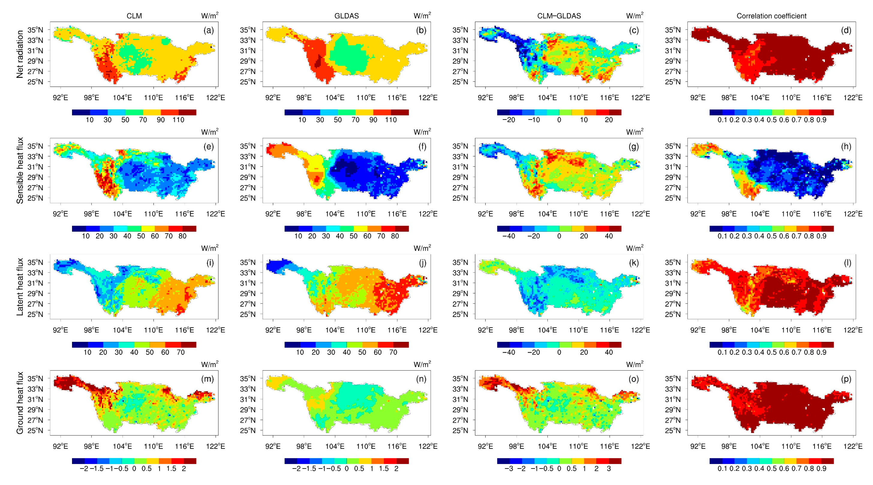
In order to further validate the simulation performance, the simulation results of water cycle and energy balance process elements were interpolated to a spatial resolution of 0.25 degrees and compared with GLDAS-Noah data. Figure 6 shows the spatial distribution of the mean energy fluxes, including net radiation, sensible heat flux, latent heat flux, and soil heat flux output from CLM and Noah during 1979–2015, the differences between the two results, and the correlation coefficient of the two series. It can be seen from the figure that the spatial distribution of the simulated values of these four elements was relatively consistent with the observed values, and the net radiation was the highest in the Jinsha River Basin, reaching more than 90 W/m2, which was related to the higher altitude and drier air. The spatial distribution of sensible heat flux and latent heat flux was exactly the opposite. Due to the high altitude and dry climate in the source region of the Yangtze River, the soil temperature and humidity were low, the evaporable water was relatively small, and it was not easy to vaporize to absorb heat, but convert most of the net radiation into sensible heat. The opposite was true in the middle and lower reaches of the Yangtze River Basin. The soil heat flux, which was mainly calculated according to the principle of surface energy balance in the model, was relatively small and had little spatial difference. Except for sensible heat flux, the spatial correlation coefficients of the other energy fluxes were high, indicating that the CLM simulation results had high similarity with GLDAS-Noah, especially in most regions below the Jinsha River Basin.
Figure 7 shows the spatial distribution of soil moisture derived from CLM and GLDAS-Noah at soil depths of 10, 40, 100 and 200 cm. It can be seen that the spatial distribution of the two was relatively consistent, showing a decreasing spatial distribution from southeast to northwest. The soil moisture in the middle and lower reaches of the basin was relatively high, mostly between 0.3 and 0.4 mm3/mm3, while the headwater region was lower, less than 0.2 mm3/mm3. The spatial distribution of soil moisture was highly consistent at soil depths of 10, 40, and 100 cm, indicating that the spatial distribution of soil moisture was not greatly affected by soil depth within 1 m. However, at a soil depth of 200 cm, the soil moisture of CLM in parts of the Sichuan Basin had decreased while it was increased with GLDAS-Noah, resulting in a large bias in the region. From the perspective of simulation bias, except for the Han River Basin and Jinsha River Basin, the simulation in other regions was relatively low. The deviation in the middle and lower reaches within 100 cm of soil depth ranged from −0.05 to 0.05 mm3/mm3, and the deviation distribution of surface soil moisture was similar to that of latent heat flux in Figure 6, indicating that evapotranspiration was closely related to surface soil moisture. However, the deviation was further increased at 200 cm of soil depth, ranging from −0.1 to 0 mm3/mm3. From the perspective of the correlation coefficient, with the increase in soil depth, the correlation coefficient increased. The highest correlation coefficient was found in the lower Jinsha River Basin, followed by Dongting Lake and Poyang Lake, and the correlation coefficient was poor in other regions.
Overall, the energy fluxes and soil water fluxes of CLM and GLDAS-Noah had good consistency in spatial distribution. However, because the atmospheric forcing data CMFD used in this paper was different from that used in GLDAS-Noah, and the structures of the CLM and Noah and the parameterization schemes for calculating sensible heat and soil water were also different, the sensible heat flux and soil water fluxes were less correlated. In addition, the spatial resolution of CLM was 0.1 degrees, and that of GLDAS-Noah was 0.25 degrees. In order to facilitate the comparison between the two, the results derived from CLM are interpolated, which may also cause bias.
3.3. Influence of Artificial Water Withdrawal on Water Cycle Process
3.3.1. Variation of Groundwater Table Depth
Figure 8 shows the spatial distribution of average annual groundwater table depth and its variation and groundwater consumption from 1981 to 2010. The distribution of groundwater table depth was consistent with the topographical distribution of the Yangtze River Basin. The groundwater table depth in the plains was shallow, and the shallowest point did not exceed 3 m, while it was deep in the hilly regions, and the deepest point could reach more than 10 m. Due to the large urban population density, high industrialization, and more arable land in the plains, the water consumption was much greater than that in the hilly regions. After artificial water withdrawal, groundwater resources were used to meet the needs of agricultural and industrial development, human life and the ecosystem, resulting in increased groundwater table depth. As shown in Figure 8c, the groundwater table depth in most regions increased by 0.1–0.3 m. It increased significantly in the regions with a large water consumption demand, such as the Yangtze River Delta urban agglomeration, which was highly consistent with the spatial distribution of groundwater consumption in Figure 8d. However, some areas in the upper reaches of the Jinsha River and Jialing River have seen groundwater recovery. The reason was that these areas had fewer water resources and could not meet their own water demand. In the model, the deficit water was obtained from the surrounding grid cells, and the remaining wastewater was directly discharged into the grid cell after water consumption, which further recharged the groundwater and led to groundwater recovery.
3.3.2. Variation in Soil Moisture
Surface soil moisture is most significantly affected by climate change and human activities and is also closely related to land surface and hydrological elements such as evapotranspiration and runoff. Therefore, the variation of surface soil moisture was mainly concerned. Figure 9 shows the spatial distribution of average annual surface soil moisture and its variation and the agricultural water consumption from 1981 to 2010. The soil moisture in the basin below the Jinsha River was relatively high, ranging from 0.25 to 0.4 mm3/mm3. The climate of the upper reaches was dry, the soil was mostly alpine soil, and the soil moisture was low, generally not more than 0.2 mm3/mm3. The plains in the middle and lower reaches of the Yangtze River Basin and the Sichuan Basin in the upper reaches of the Yangtze River Basin had a large area of arable land, resulting in a large amount of agricultural water consumption, with an annual average of more than 50 mm. Since there was very little arable land in the Jinsha River Basin, the agricultural water consumption was also very small, with an annual average of not more than 2 mm. Agricultural irrigation had significantly changed the state of soil moisture, and soil moisture had increased by 0–0.03 mm3/mm3 in most areas. In the commercial grain production bases such as the Western Sichuan Plain, Jianghan Plain, Dongting Lake Plain, and Taihu Plain, the soil moisture increased by 0.03–0.05 mm3/mm3, which corresponded to the area with large agricultural water consumption in Figure 9d. However, soil moisture decreased in some grid cells, which basically corresponded to the grid cells with decreased groundwater table depth in Figure 8c. It can be seen from Figure 8a that the groundwater table depth in this area was deep below the 10th soil layer of the model, and the bottom soil recharged the groundwater in the form of gravity drainage, which was the main reason for the decrease in soil moisture.
3.3.3. Variation in Discharge
In this paper, it was assumed that the variation of measured discharge was the result of the combined effects of climate change, land use change and artificial water withdrawal. The variation in discharge in Experiment 1 was the result of climate change, while the variation in discharge in Experiment 2 was the result of the combined effects of climate change and artificial water withdrawal. Therefore, the contribution rate of each factor to the variation in discharge could be separated by comparing the results of each experiment. Table 5 listed the contribution rate of various factors to the variation of discharge of 15 hydrological stations in the Yangtze River Basin. Due to the different lengths of the measured data of each station, the time series were selected as 1979–2000 for convenience.
It can be seen from Table 5 that during the period from 1979 to 2000, climate change played a dominant role in the variation of discharge in the Yangtze River Basin, leading to an increase in discharge at most stations. Artificial water withdrawal reduced discharge, and its contribution was low. In addition, the contribution rate of land use change cannot be ignored, which led to a reduction in discharge at most stations. In general, the discharge in the Jinsha River Basin, Dongting Lake and Poyang Lake has been greatly increased due to the influence of climate change, which was also the main reason for the increase in discharge in the downstream mainstream.
4. Discussion
4.1. Attribution Analysis of Soil Moisture Change
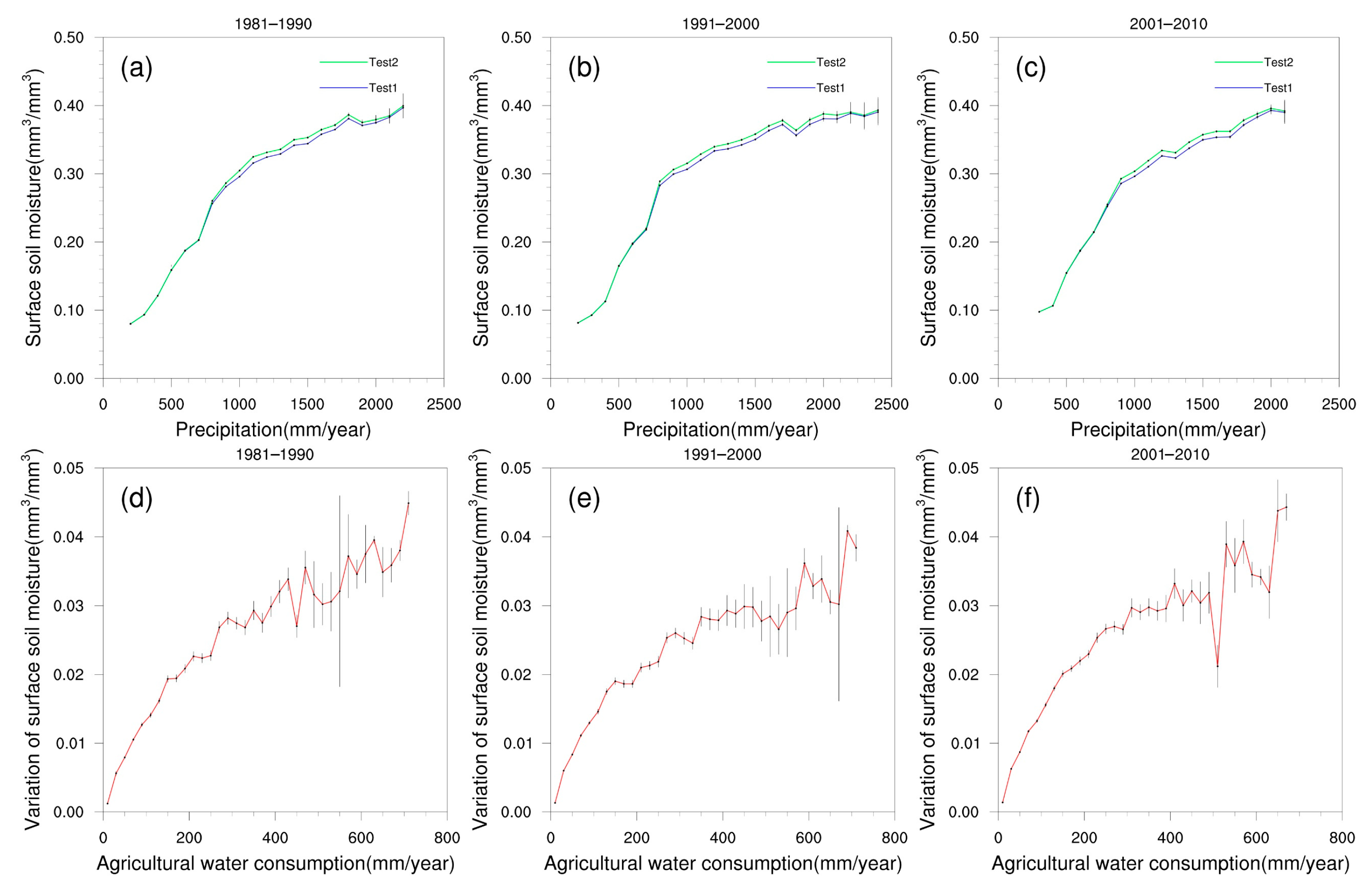
Soil moisture controls the water and heat exchange between the land surface and atmosphere and affects the evaporation and runoff in the water cycle. Therefore, soil moisture was the research focus of the land surface process. In order to further explore the effect of agricultural water consumption on the variation of surface soil moisture, the agricultural water consumption of 20 mm/year was taken as the statistical interval, and the variation in soil moisture in different agricultural water consumption intervals was counted with the grid cell as the unit. At the same time, in order to consider the influence of climate change, 100 mm/year of precipitation was taken as the statistical interval, and the relationship between precipitation and soil moisture in different decades was calculated (Figure 10). In Figure 10a–c, the abscissa was the different precipitation intervals in the two experiments, the ordinate was the average soil moisture in each precipitation interval, and the black line represented the range of standard error of soil moisture in each statistical interval. Similarly, in Figure 10d–f, the abscissa was the different agricultural water consumption intervals, the ordinate was the average variation of soil moisture in each agricultural water consumption interval, and the black line represented the range of standard error of soil moisture change in each statistical interval.
According to Figure 10a–c, the precipitation in the 1990s was the highest, followed by the 1980s and the 2000s. No matter which decade, soil moisture increased with the increase in precipitation, and the variation in soil moisture increased with the increase in agricultural water consumption. In the same decade, agricultural irrigation significantly increased soil moisture only in areas where precipitation exceeded a certain range. In the 1980s and 1990s, the humidification effect of agricultural irrigation was more obvious in areas where precipitation was greater than 800 mm/year, while in the 2000s, the humidification effect was more significant in areas where precipitation was greater than 900 mm/year. Areas where precipitation was less than 800 mm/year highly coincided with areas where agricultural water consumption was less than 30 mm/year. The increase in soil moisture caused by agricultural irrigation in this area was small, not exceeding 0.01 mm3/mm3. In fact, it can be seen from Figure 10d–f that in areas where agricultural water consumption was less than 150 mm/year, the variation in soil moisture was not large, the maximum was not more than 0.02 mm3/mm3, and there were no obvious differences among the three decades. In areas where agricultural water consumption was between 150 and 400 mm/year, the variation in soil moisture began to be different between decades. The variation in soil moisture was the largest in the 2000s, followed by the 1980s and 1990s. In areas where agricultural water consumption was greater than 400 mm/year, the variation in soil moisture showed great fluctuations in the three decades. This was because there were few grid cells of agricultural water consumption above 400 mm/year in the same statistical interval of different decades. Therefore, the statistical results showed some deviation, and the standard error increased significantly.
In general, agricultural irrigation did not significantly increase soil moisture in areas where agricultural water consumption was less than 150 mm/year. In areas where the agricultural water consumption was greater than 150 mm/year, agricultural irrigation can significantly humidify the soil, and the variation in soil moisture was different between decades, while the differences were not obvious, indicating that agricultural irrigation was still the main reason for the variation in soil moisture.
4.2. Modeling Uncertainties
Although the CLM4.5 land surface model had a good performance in simulating the water cycle process over the Yangtze River Basin, it was still worthwhile to explore the uncertainties of the modeling results. First, the simulated discharge showed a slight underestimation in the upper reaches, especially in winter, which indicated that the model could be improved in terms of precipitation identification and snowmelt mechanism. In addition, a large number of reservoirs had been built in the Yangtze River Basin. However, the regulation of the reservoirs was not considered in the CLM4.5 model, which also brought uncertainty to the discharge simulation. Secondly, vegetation had an important influence on the water and energy fluxes. However, dynamic changes in vegetation were not considered in the model, which resulted in a certain deviation of sensible heat and soil moisture. Finally, the time step of the model was 30 min, while the temporal resolution of the atmospheric forcing data was 3 h, which created uncertainty in the temporal interpolation. Therefore, a new module that considered the reservoir operation process and the dynamic change of vegetation is likely to be developed, and a high-resolution input dataset is needed to carry out future research.
5. Conclusions
An artificial water withdrawal scheme was developed and coupled with the CLM4.5 land surface model to assess the impact of water consumption on the water cycle process in the Yangtze River Basin. Two experiments were conducted to analyze the variation in groundwater table depth, surface soil moisture, as well as the contribution of climate change, LUCC and artificial water withdrawal to discharge. The following conclusions can be reached:
(1) A parameterization scheme of artificial water withdrawal considering the process of water intake, water use and drainage was developed. Based on the socio-economic data and water consumption data of cities in the Yangtze River Basin, a rasterized water consumption dataset of the Yangtze River Basin was established. Compared with the data of the Yangtze River Basin Water Resources Bulletin, the maximum annual water consumption error was not more than ±10%, and the data accuracy can meet the needs.
(2) The Nash efficiency coefficients (NSE) of the monthly discharge of the 15 hydrological stations ranged from 0.66 to 0.96, and the relative error (PBIAS) ranged from −13.5% to 16.5%. Overall, the model can well reflect the discharge process of the mainstream and tributaries of the Yangtze River Basin.
(3) For the surface energy flux, the simulated values of net radiation, latent heat, and soil heat flux were in good agreement with the observed values except for sensible heat. For the soil water flux, the spatial distribution of the simulated and observed soil moisture at different depths was consistent, while the soil moisture was underestimated. The differences in atmospheric forcing data, model structure and the parameterization scheme may be the main reason for the errors between the simulated and observed results.
(4) Artificial water withdrawal led to a 0.1–0.3 m increase in groundwater table depth in most areas of the basin, which led to an increase in soil moisture in the corresponding areas. In areas where agricultural water consumption was less than 150 mm/year, agricultural irrigation did not significantly increase soil moisture. In areas where agricultural water consumption was greater than 150 mm/year, agricultural irrigation could significantly increase surface soil moisture, and the variation in soil moisture was different over the decades. Climate change was the main factor for the variation of annual discharge at most stations in the Yangtze River Basin, and the discharge of Jinsha River Basin, Dongting Lake and Poyang Lake increased more under the influence of climate change.
Author Contributions
Conceptualization, H.W. (Hejia Wang) and M.Y.; methodology, H.W. (Hao Wang); software, B.H.; validation, H.W. (Hejia Wang) and W.X.; formal analysis, B.H.; investigation, B.H.; data curation, M.Y.; writing—original draft preparation, H.W. (Hejia Wang); writing—review and editing, B.H.; visualization, M.Y.; supervision, H.W. (Hao Wang); funding acquisition, W.X. All authors have read and agreed to the published version of the manuscript.
Funding
This research was funded by the National Natural Science Foundation of China, grant number 51779271.
Data Availability Statement
The data used in this study are available on request from the corresponding author.
Acknowledgments
The authors are grateful to their colleagues at the National SuperComputer Center in Tianjin for their help porting and running the CLM4.5 model.
Conflicts of Interest
The authors declare no conflict of interest.
References
- Wang, Y.H.; Liao, W.H.; Ding, Y.; Wang, X.; Jiang, Y.Z.; Song, X.S.; Lei, X.H. Water resource spatiotemporal pattern evaluation of the upstream Yangtze River corresponding to climate changes. Quat. Int. 2015, 380–381, 187–196. [Google Scholar] [CrossRef]
- Zhou, X.Y.; Lei, K. Influence of human-water interactions on the water resources and environment in the Yangtze River Basin from the perspective of multiplex networks. J. Clean. Prod. 2020, 265, 121783. [Google Scholar] [CrossRef]
- Cao, L.J.; Zhang, Y.; Shi, Y. Climate change effect on hydrological processes over the Yangtze River basin. Quat. Int. 2011, 244, 202–210. [Google Scholar] [CrossRef]
- Xu, J.J.; Yang, D.W.; Yi, Y.H.; Lei, Z.D.; Chen, J.; Yang, W.J. Spatial and temporal variation of runoff in the Yangtze River basin during the past 40 years. Quat. Int. 2008, 186, 32–42. [Google Scholar] [CrossRef]
- Xu, X.B.; Yang, G.S.; Tan, Y.; Liu, J.P.; Hu, H.Z. Ecosystem services trade-offs and determinants in China’s Yangtze River Economic Belt from 2000 to 2015. Sci. Total Environ. 2018, 634, 1601–1614. [Google Scholar] [CrossRef]
- Yang, D.W.; Yang, Y.T.; Xia, J. Hydrological cycle and water resources in a changing world: A review. Geogr. Sustain. 2021, 2, 115–122. [Google Scholar]
- Döll, P.; Kaspar, F.; Lehner, B. A global hydrological model for deriving water availability indicators: Model tuning and validation. J. Hydrol. 2003, 270, 105–134. [Google Scholar] [CrossRef]
- Rodrigo, C.D.; Water, C.; Diogo, C.B. Validation of a full hydrodynamic model for large-scale hydrologic modelling in the Amazon. Hydrol. Process. 2013, 27, 333–346. [Google Scholar]
- Sellers, P.J.; Mintz, Y.; Sud, Y.C.; Dalcher, A. A simple biosphere model (SiB) for use within general circulation models. J. Atmos. Sci. 1986, 43, 505–531. [Google Scholar] [CrossRef]
- Sellers, P.J.; Randall, D.A.; Collatz, G.J.; Berry, J.A.; Field, C.B.; Dazlich, D.A.; Zhang, C.; Collelo, G.D.; Bounoua, L. A revised land surface parameterization (SiB2) for atmospheric GCMs. Part I: Model formulation. J. Clim. 1996, 9, 676–705. [Google Scholar] [CrossRef]
- Dai, Y.J.; Zeng, Q.C. A land surface model (IAP94) for climate studies. Part I: Formulation and validation in off-line experiments. Adv. Atmos. Sci. 1997, 14, 433–460. [Google Scholar]
- Dai, Y.J.; Zeng, X.B.; Dickinson, R.E.; Baker, I.; Bonan, G.B.; Bosilovich, M.G.; Denning, S.; Dirmeyer, P.; Houser, P.R.; Niu, G.Y.; et al. The common land model. Bull. Am. Meteorol. Soc. 2003, 84, 1013–1023. [Google Scholar] [CrossRef] [Green Version]
- Bierkens, M.F.P. Global hydrology 2015: State, trends, and directions. Water Resour. Res. 2015, 51, 4923–4947. [Google Scholar] [CrossRef]
- Zhao, W.; Li, A.N. A review on land surface processes modelling over complex terrain. Adv. Meteorol. 2015, 2015, 607181. [Google Scholar] [CrossRef] [Green Version]
- Maayar, M.E.; Price, D.T.; Chen, J.M. Simulating daily, monthly and annual water balances in a land surface model using alternative root water uptake schemes. Adv. Water Resour. 2009, 32, 1444–1459. [Google Scholar] [CrossRef]
- Jiao, Y.; Lei, H.M.; Yang, D.W.; Huang, M.Y.; Liu, D.F.; Yuan, X. Impact of vegetation dynamics on hydrological processes in a semi-arid basin by using a land surface-hydrology coupled model. J. Hydrol. 2017, 551, 116–131. [Google Scholar] [CrossRef]
- Benoit, R.; Pellerin, P.; Kouwen, N.; Ritchie, H.; Donaldson, N.; Joe, P.; Soulis, E.D. Toward the use of coupled atmospheric and hydrologic models at regional scale. Mon. Weather Rev. 2000, 128, 1681–1706. [Google Scholar] [CrossRef]
- Chen, F.; Xie, Z.H. Effects of interbasin water transfer on regional climate: A case study of the Middle Route of South-to-North Water Transfer Project in China. J. Geophys. Res. 2010, 115, D11112. [Google Scholar] [CrossRef] [Green Version]
- Zou, J.; Xie, Z.H.; Zhan, C.S.; Qin, P.H.; Sun, Q.; Jia, B.H.; Xia, J. Effects of anthropogenic groundwater exploitation on land surface processes: A case study of the Haihe River Basin, northern China. J. Hydrol. 2015, 524, 625–641. [Google Scholar] [CrossRef]
- Zou, J.; Xie, Z.H.; Yu, Y.; Zhan, C.S.; Sun, Q. Climatic responses to anthropogenic groundwater exploitation: A case study of the Haihe River Basin, Northern China. Clim. Dyn. 2014, 42, 2125–2145. [Google Scholar] [CrossRef]
- Gao, B.; Yang, D.W.; Yang, H.B. Impact of the Three Gorges Dam on flow regime in the middle and lower Yangtze River. Quat. Int. 2013, 304, 43–50. [Google Scholar] [CrossRef]
- Yang, K.; He, J.; Tang, W.J.; Qin, J.; Cheng, C. On downward shortwave and longwave radiations over high altitude regions: Observation and modeling in the Tibetan Plateau. Agric. For. Meteorol. 2010, 150, 38–46. [Google Scholar] [CrossRef]
- He, J.; Yang, K.; Tang, W.J.; Lu, H.; Qin, J.; Chen, Y.Y.; Li, X. The first high-resolution meteorological forcing dataset for land process studies over China. Sci. Data 2020, 7, 25. [Google Scholar] [CrossRef] [PubMed]
- Zeng, J.H.; Yuan, X.; Ji, P.; Shi, C.X. Effects of meteorological forcings and land surface model on soil moisture simulation over China. J. Hydrol. 2021, 603, 126978. [Google Scholar] [CrossRef]
- Stefan, S.; Verena, H.; Karen, F.; Jacob, B. Global Map of Irrigation Areas Version 5; Rheinische Friedrich-Wilhelms-University: Bonn, Germany; Food and Agriculture Organization of the United Nations: Rome, Italy, 2013. [Google Scholar]
- Center for International Earth Science Information Network-CIESIN-Columbia University. Gridded Population of the World, Version 4 (GPWv4): Population Density Adjusted to Match 2015 Revision UN WPP Country Totals, Revision 11; NASA Socioeconomic Data and Applications Center (SEDAC): Palisades, NY, USA, 2018. [Google Scholar] [CrossRef]
- Liu, H.; Jiang, D.; Yang, X.; Luo, C. Spatialization Approach to 1km Grid GDP Supported by Remote Sensing. J. Geo-Inf. Sci. 2005, 7, 120–123. [Google Scholar]
- Oleson, K.; Lawrence, D.; Bonan, G.; Drewniak, B.; Huang, M.; Koven, C.; Levis, S.; Li, F.; Riley, W.; Subin, Z. Technical Description of Version 4.5 of the Community Land Model (CLM), 1st ed.; National Center for Atmospheric Research: Boulder, CO, USA, 2013; pp. 1–11. [Google Scholar]
- Hurrell, J.W.; Holland, M.M.; Gent, P.R.; Ghan, S.; Kay, J.E.; Kushner, P.J.; Lamarque, J.F.; Large, W.G.; Lawrence, D.; Lindsay, K.; et al. The community earth system model: A framework for collaborative research. Bull. Am. Meteorol. Soc. 2013, 94, 1339–1360. [Google Scholar] [CrossRef]
- Zeng, Y.J.; Xie, Z.H.; Yu, Y.; Liu, S.; Wang, L.Y.; Zou, J.; Qin, P.H.; Jia, B.H. Effects of anthropogenic water regulation and groundwater lateral flow on land processes. J. Adv. Model. Earth Syst. 2016, 8, 1106–1131. [Google Scholar] [CrossRef]
- Wada, Y.; Wisser, D.; Bierkens, M.F.P. Global modeling of withdrawal, allocation and consumptive use of surface water and groundwater resources. Earth Syst. Dyn. 2014, 5, 15–40. [Google Scholar] [CrossRef] [Green Version]
- Qin, D.Y.; Lu, C.Y.; Liu, J.H.; Wang, H.; Wang, J.H.; Li, H.H.; Chu, J.Y.; Chen, G.F. Theoretical framework of dualistic nature–social water cycle. Chin. Sci. Bull. 2014, 59, 810–820. [Google Scholar] [CrossRef]
- Lu, S.B.; Zhang, X.L.; Bao, H.J.; Skitmore, M. Review of social water cycle research in a changing environment. Renew. Sustain. Energy Rev. 2016, 63, 132–140. [Google Scholar] [CrossRef] [Green Version]
- Nash, J.E.; Sutcliffe, J.V. River flow forecasting through conceptual models part I—A discussion of principles. J. Hydrol. 1970, 10, 282–290. [Google Scholar] [CrossRef]
- Gupta, H.V.; Sorooshian, S.; Yapo, P.O. Status of automatic calibration for hydrologic models: Comparison with multilevel expert calibration. J. Hydrol. Eng. 1999, 4, 135–143. [Google Scholar] [CrossRef]
Figure 1.
Topography and river stream of the Yangtze River Basin.

Figure 2.
Artificial water withdrawal scheme.

Figure 3.
Spatial distribution of average annual water consumption in the Yangtze River Basin.

Figure 4.
Validation of water consumption data in the Yangtze River Basin.

Figure 5.
Simulated and observed discharge process of main hydrological stations in the Yangtze River Basin. (a) Xiaodeshi, (b) Pingshan, (c) Gaochang, (d) Lijiawan, (e) Beibei, (f) Cuntan, (g) Wulong, (h) Yichang, (i) Changyang, (j) Baihe, (k) Taoyuan, (l) Xiangtan, (m) Shishang, (n) Meigang, (o) Datong.

Figure 6.
Spatial distribution of mean energy flux elements of CLM and GLDAS-Noah. (a,e,i,m) is net radiation, sensible heat flux, latent heat flux and ground heat flux for CLM. (b,f,j,n) is net radiation, sensible heat flux, latent heat flux and ground heat flux for GLDAS. (c,g,k,o) is the differences of net radiation, sensible heat flux, latent heat flux and ground heat flux between CLM and GLDAS. (d,h,l,p) is the correlation coefficient of net radiation, sensible heat flux, latent heat flux and ground heat flux between CLM and GLDAS.

Figure 7.
Spatial distribution of soil moisture of CLM and GLDAS-Noah at different soil depths. (a,e,i,m) is soil moisture for CLM at 10, 40, 100 and 200 cm. (b,f,j,n) is soil moisture for GLDAS at 10, 40, 100 and 200 cm. (c,g,k,o) is the differences of soil moisture between CLM and GLDAS at 10, 40, 100 and 200 cm. (d,h,l,p) is the correlation coefficient of soil moisture between CLM and GLDAS at 10, 40, 100 and 200 cm.

Figure 8.
Spatial distribution of groundwater consumption, groundwater table depth and its variation. (a) is groundwater table depth for experiment1. (b) is groundwater table depth for experiment2. (c) is the difference of groundwater table depth between experiment1 and experiment2. (d) is mean annual groundwater consumption.

Figure 9.
Spatial distribution of agricultural water consumption, surface soil moisture and its variation. (a) is Surface soil moisture for experiment1. (b) is surface soil moisture for experiment2. (c) is the difference of surface soil moisture between experiment1 and experiment2. (d) is mean annual agricultural water consumption.

Figure 10.
Effects of precipitation and agricultural water consumption on surface soil moisture and its changes. The relationship between precipitation and soil moisture in (a) 1980s, (b) 1990s and (c) 2000s. The relationship between agricultural water consumption and variation of surface soil moisture in (d) 1980s, (e) 1990s and (f) 2000s.


Table 1.
Main hydrological stations of the mainstream and tributaries of the Yangtze River Basin.
| Station | Longitude (°) | Latitude (°) | Subbasin | Period |
|---|---|---|---|---|
| Xiaodeshi | 101.87 | 26.72 | Yalong River Basin | 1979–2010 |
| Pingshan | 104.17 | 28.65 | Jinsha River Basin | 1979–2011 |
| Gaochang | 104.42 | 28.81 | Min River Basin | 1979–2012 |
| Lijiawan | 104.97 | 29.13 | Tuo River Basin | 1979–2000 |
| Beibei | 106.46 | 29.81 | Jialing River Basin | 1979–2015 |
| Cuntan | 106.6 | 29.62 | Upper Yangtze River Basin | 1979–2015 |
| Wulong | 107.75 | 29.32 | Wu River Basin | 1979–2015 |
| Yichang | 111.28 | 30.69 | Upper Yangtze River Basin | 1979–2015 |
| Changyang | 111.18 | 30.48 | Qing River Basin | 1979–2000 |
| Baihe | 110.11 | 32.83 | Han River Basin | 1979–2000 |
| Taoyuan | 111.49 | 28.92 | Yuan River Basin | 1979–2000 |
| Xiangtan | 112.93 | 27.87 | Xiang River Basin | 1979–2000 |
| Shishang | 115.72 | 28.18 | Gan River Basin | 1979–2000 |
| Meigang | 116.82 | 28.44 | Xin River Basin | 1979–2000 |
| Datong | 117.63 | 30.77 | Lower Yangtze River Basin | 1979–2006 |
Table 2.
Land surface simulation experiments in the Yangtze River Basin.
| Experiment | Simulation Period | Artificial Water Withdrawal |
|---|---|---|
| Experiment 1 | 1981–2010 | No |
| Experiment 2 | 1981–2010 | Yes |
Table 3.
Parameters, meanings and calibrated values of CLM model.
| Parameter | Meaning | Calibrated Value |
|---|---|---|
| dewmx | Maximum dew | 0.1 |
| hksat | Hydraulic conductivity at saturation | 0.005 |
| porosity | Soil porosity | 0.5 |
| sucsat | Minimum soil suction | 250 |
| wtfact | Fraction of model area with high water table | 0.3 |
| bsw | Clapp and hornbereger “b” parameter | 5 |
| wimp | Water impermeable if porosity less than wimp | 0.05 |
| zlnd | Roughness length for soil | 0.01 |
| pondmx | Ponding depth | 10 |
| csoilc | Drag coefficient for soil under canopy | 0.004 |
| zsno | Roughness length for snow | 0.0024 |
| capr | Tuning factor to turn first layer T into surface T | 0.34 |
| cnfac | Crank–Nicholson factor between 0 and 1 | 0.375 |
| z0m | Aerodynamic roughness length | 0.175 |
| ssi | Irreducible water saturation of snow | 0.035 |
Table 4.
Simulation performance of discharge process at 15 hydrological stations in the Yangtze River Basin.
Table 4.
Simulation performance of discharge process at 15 hydrological stations in the Yangtze River Basin.
| Station | Subbasin | NSE | PBIAS |
|---|---|---|---|
| Xiaodeshi | Yalong River Basin | 0.66 | −12.2% |
| Pingshan | Jinsha River Basin | 0.74 | −13.5% |
| Gaochang | Min River Basin | 0.86 | −11.9% |
| Lijiawan | Tuo River Basin | 0.81 | 10.8% |
| Beibei | Jialing River Basin | 0.87 | 2.8% |
| Cuntan | Upper Yangtze River Basin | 0.87 | −9.3% |
| Wulong | Wu River Basin | 0.89 | 2.8% |
| Yichang | Upper Yangtze River Basin | 0.88 | −6.9% |
| Changyang | Qing River Basin | 0.89 | 16.5% |
| Baihe | Han River Basin | 0.81 | −1.8% |
| Taoyuan | Yuan River Basin | 0.94 | 7.5% |
| Xiangtan | Xiang River Basin | 0.92 | 1.9% |
| Shishang | Gan River Basin | 0.86 | 4.4% |
| Meigang | Xin River Basin | 0.96 | −3.2% |
| Datong | Lower Yangtze River Basin | 0.77 | 1.8% |
Table 5.
The contribution rate of various factors to the variation in the discharge of 15 hydrological stations in the Yangtze River Basin.
Table 5.
The contribution rate of various factors to the variation in the discharge of 15 hydrological stations in the Yangtze River Basin.
| Station | Climate Change | Artificial Water Withdrawal | LUCC | Discharge Change | |||
|---|---|---|---|---|---|---|---|
| Value (m3/s) | Contribution (%) | Value (m3/s) | Contribution (%) | Value (m3/s) | Contribution (%) | Value (m3/s) | |
| Xiaodeshi | 12.8 | 77.3 | −0.003 | 0.0 | 3.7 | 22.7 | 16.5 |
| Pingshan | 43.9 | 90.6 | −0.078 | 0.2 | −4.5 | 9.2 | 39.4 |
| Gaochang | −0.7 | 6.5 | −0.337 | 3.2 | −9.5 | 90.3 | −10.5 |
| Lijiawan | −3.7 | 80.8 | −0.163 | 3.6 | −0.7 | 15.6 | −4.5 |
| Beibei | −14.6 | 31.6 | −0.089 | 0.2 | −31.6 | 68.2 | −46.3 |
| Cuntan | 16.8 | 55.0 | −0.002 | 0.0 | −13.8 | 45.0 | 3.1 |
| Wulong | 22.0 | 82.9 | −0.694 | 2.6 | −3.8 | 14.5 | 17.5 |
| Yichang | 8.7 | 57.7 | −0.519 | 3.5 | −5.8 | 38.8 | 2.3 |
| Changyang | −4.2 | 60.0 | −0.001 | 0.0 | 2.8 | 40.0 | −1.4 |
| Baihe | −11.1 | 38.6 | −0.021 | 0.1 | −17.7 | 61.4 | −28.8 |
| Taoyuan | 33.4 | 73.3 | −0.375 | 0.8 | −11.8 | 25.9 | 21.2 |
| Xiangtan | 44.6 | 68.4 | −1.135 | 1.7 | −19.4 | 29.8 | 24.0 |
| Shishang | 28.6 | 58.9 | −0.448 | 0.9 | −19.5 | 40.2 | 8.6 |
| Meigang | 12.5 | 91.6 | −0.090 | 0.7 | 1.1 | 7.7 | 13.4 |
| Datong | 251.5 | 66.4 | −0.650 | 0.2 | −126.5 | 33.4 | 124.4 |
Publisher’s Note: MDPI stays neutral with regard to jurisdictional claims in published maps and institutional affiliations. |
© 2022 by the authors. Licensee MDPI, Basel, Switzerland. This article is an open access article distributed under the terms and conditions of the Creative Commons Attribution (CC BY) license (https://creativecommons.org/licenses/by/4.0/).
Share and Cite
MDPI and ACS Style
Wang, H.; Hou, B.; Yang, M.; Xiao, W.; Wang, H. Effects of Artificial Water Withdrawal on the Terrestrial Water Cycle in the Yangtze River Basin. Water 2022, 14, 3117. https://doi.org/10.3390/w14193117
AMA Style
Wang H, Hou B, Yang M, Xiao W, Wang H. Effects of Artificial Water Withdrawal on the Terrestrial Water Cycle in the Yangtze River Basin. Water. 2022; 14(19):3117. https://doi.org/10.3390/w14193117
Chicago/Turabian StyleWang, Hejia, Baodeng Hou, Mingxiang Yang, Weihua Xiao, and Hao Wang. 2022. "Effects of Artificial Water Withdrawal on the Terrestrial Water Cycle in the Yangtze River Basin" Water 14, no. 19: 3117. https://doi.org/10.3390/w14193117
Note that from the first issue of 2016, this journal uses article numbers instead of page numbers. See further details here.