Numerical Modeling of COD Transportation in Liaodong Bay: Impact of COD Loads from Rivers Flowing into the Sea

Abstract

Pollution loads pose a major threat to the health of the marine environment and the long-term viability of the coastal economy. The present study developed a coupling model to simulate the chemical oxygen demand (COD) transport in upper rivers (1D) and subsequent diffusion in the coastal zone (2D) in Liaodong Bay, based on the HydroInfo system. Three main seagoing rivers, including Daliao, Liao, and Daling Rivers, were selected and investigated for hydrodynamic and hydrochemical analyses. The mathematical model was evaluated by monitoring data from state-controlled cross-sections scattered along the three rivers, and the observation data showed good agreement with simulated values, confirming the model’s accuracy in terms of spatial and temporal distribution. The transport and propagation process of COD in inlet rivers, such as Daliao, Liao, and Daling, including the sea area of Liaodong Bay, were simulated and analyzed. Simulated results revealed that the pollution range of COD in Liaodong Bay was 258–391 km² in different seasons. The pollutant leakage scenarios for the three rivers entering the sea were simulated utilizing the developed mathematical model. The study simulated and predicted that, in the event of a sudden water pollution accident (e.g., sneak discharge and leakage at various sections of sea-entering rivers, such as Daliao, Liao, and Daling), pollutants might take 2–11 days to reach the sea-entering mouth, and the sea area would take 8–32 days to reach the maximum pollution range. Our numerical modeling may be used to analyze and make decisions on pollution control in Liaodong Bay and major sea-entry rivers, and be useful to water environment management in sea-entry rivers and Liaodong Bay, and water pollution emergency responses.

1. Introduction

The eastern coast is the most dynamic and fastest-growing region in China. With rapid economic and social development, a large amount of urban and rural sewage from coastal areas is discharged into the sea through entering rivers [1], seriously threatening the ecological safety and economic development of seas [2]. Chemical oxygen demand (COD) is an indicator of the amount of reducing substances in water, which is generally employed to represent the total amount of organic substances in wastewater. Both COD and TOC could be selected for simulation, but our main purpose was to verify the effectiveness of the simulation method. Moreover, in the water quality evaluation system of surface water and seawater, COD is regarded as an important water quality evaluation index, and many scholars pay attention to the influence of COD concentration in surface water on the change of COD concentration in marine water, so we chose COD as the target pollutant in this simulation. COD is an essential component in determining how to respond to the pollution state of marine waterways [3]. It is also a factor in determining how to reduce pollution in marine regions at a national level. The interplay of sea and land in nearshore waters, the complex hydrodynamic environment, and the land–sea ecology are influenced by interconnected physical, chemical, and biological factors, all adding to the uncertainty of water quality forecasts. Given that the problem of offshore pollution worsens as coastal business and society develops [4], investigating the impact of COD from rivers entering the sea on near-shore waters, and utilizing this information to design pollution reduction methods are critical [5,6]. Due the complexity mentioned above, it is relatively difficult to simulate and predict COD concentration changes by the general linear prediction model, necessitating the adoption of a numerical model with a coupling mechanism.

Scholars in the United States and overseas have conducted many studies which have shown the contamination of near-shore marine regions caused by rivers entering into the sea. Mike21, DelftT3D and other measurement methods were used to establish a hydrodynamically derived pollutant transport model in the sea region. Scholars have also extensively investigated the distribution features of COD, dissolved oxygen (DO), eutrophication, petroleum species, and heavy metals in sea areas [7,8,9,10,11,12,13]. Accurately predicting the scope of COD impact of rivers into seas, and the effects of sudden water pollution events in rivers flowing into seas using the remote sensing of water quality and field monitoring is difficult. The HYDROINFO numerical simulation model is a complete simulation software created independently by the Dalian University of Technology. It may be used to simulate water environment conditions in rivers, estuaries, near-shore seas, oceans, and other water environments. It also features easy and versatile pre- and post-processing functions, data extraction functions, quick computation speeds, and broad application ranges. Researchers have utilized the HYDROINFO numerical simulation model to simulate pollution incidents in the Songhua River basin and to accurately predict the dispersion time of pollutants. Moreover, saltwater intrusion in the Pearl River was also investigated through the HYDROINFO model and obtained analytical results which showed good agreement with actual monitoring ones.

Our goal was to create a numerical simulation model by employing the HYDROINFO system for Liaodong Bay and its inlet rivers, which could mimic the near-shore water environment in Liaodong Bay and produce accurate predictions and forecasts in the event of pollutant leakage. Liaodong Bay is a semi-enclosed bay with seawater having poor self-purification ability [14]. With the growth of Dalian, Huludao, Yingkou, Jinzhou, Panjin, and other coastal cities and towns, a considerable number of pollutants enter Liaodong Bay via rivers, causing the water quality in the bay entrance to deteriorate. COD, which accounts for more than 90% of the contaminants delivered by rivers into seas, is the most common [15,16]. As a result, COD was chosen as the characteristic index. The transport process of COD in rivers and sea areas, the influence range of sea area pollution, the time of pollutants reaching the sea inlet and the maximum pollution range of sea area in the event of a sudden pollutant leakage in various rivers were simulated. Our findings may be used as a scientific foundation for pollution control in Liaodong Bay and major rivers into seas, for water environment management in rivers into seas and Liaodong Bay, and water pollution emergency responses.

2. Theory and Numerical Simulation Method

The HYDROINFO system was used to create a combined 1D and 2D hydrodynamic and water quality model of Liaodong Bay and the key inflow rivers for this research [17,18,19].

2.1. D hydrodynamic Model Construction

The scope of the 1D hydrodynamic model was the lower reaches of Daliao, Liao, and Daling Rivers. For the 1D river solution issue, the model uses a semi-implicit finite element approach [20,21,22]. This approach is used to solve the water depth and flow of the river channel independently; it iteratively computes the coupling connection between the two, which may significantly enhance calculation efficiency [23]. The finite element approach is used to combine the river level equation and the branching point water depth equation into a generic equation that is stable and converges well [24,25].

(1)

System of St. Venant equations

Continuous equation:

$$\frac{\partial \mathrm{A}}{\partial \mathrm{t}}+\frac{\partial \mathrm{Q}}{\partial \mathrm{S}}{=\mathrm{q}+\mathsf{\delta }\mathrm{Q}}_{\mathrm{c}}$$

(1)

Equation of motion:

$$\frac{\partial \mathrm{Q}}{\partial \mathrm{t}}+\frac{\partial {(\mathrm{Q}}^2/\mathrm{A})}{\partial \mathrm{S}}=-\mathrm{gA}\frac{\partial \mathrm{z}}{\partial \mathrm{S}}-\mathrm{gA}\frac{{\mathrm{Q}}^2}{{\mathrm{K}}^2}$$

(2)

(2)

Branch point connection equation

Nodal mass conservation:

$$\frac{\partial \mathsf{\Omega }}{\partial \mathrm{t}}{=\mathrm{A}}_{\mathrm{c}}\frac{\partial \mathrm{z}}{\partial \mathrm{t}}={{\displaystyle \sum }}^{}{\mathrm{Q}}_{\mathrm{i}}$$

(3)

where Ω is the storage capacity, z is the water level, ${\mathrm{A}}_{\mathrm{c}}$ is the area for water storage, ${\mathrm{Q}}_{\mathrm{i}}$ is the access to branching traffic, Z is the branch point water depth, i is the cross-section of a river channel.

2.2. D hydrodynamic Model Construction

(1)

Shallow water equation

The motion of a large-scale free fluid was simulated [26,27,28], and the fluid’s scale of motion in the pendent direction was generally and considerably less than the plane scale [29,30,31], necessitating the use of shallow water assumption to simplify conservation equations [28]. To complete the averaging process, the pressure in the vertical direction adhered to the distribution criteria for hydrostatic pressure [29], whereas the mass and momentum conservation equations were integrated in the vertical direction [32,33,34,35,36].

Continuous equation:

$$\frac{\partial \mathrm{H}}{\partial \mathrm{t}}+\frac{\partial \mathrm{Hu}}{\partial \mathrm{x}}+\frac{\partial \mathrm{Hv}}{\partial \mathrm{y}}=0$$

(4)

Motion equations:

$$\frac{\partial \mathrm{Hu}}{\partial \mathrm{t}}+\frac{\partial \left(\mathrm{Huu}\right)}{\partial \mathrm{x}}+\frac{\partial \left(\mathrm{Hvu}\right)}{\partial \mathrm{y}}=-\mathrm{gH}\frac{\partial \mathsf{\varsigma }}{\partial \mathrm{x}}-\mathrm{gu}\frac{\sqrt{{\mathrm{u}}^2{+\mathrm{v}}^2}}{{\mathrm{C}}^2}+\mathsf{\epsilon }(\frac{\partial {}^2\mathrm{Hu}}{\partial {\mathrm{x}}^2}+\frac{\partial {}^2\mathrm{Hu}}{\partial {\mathrm{y}}^2})$$

(5)

$$\frac{\partial \mathrm{Hv}}{\partial \mathrm{t}}+\frac{\partial \left(\mathrm{Huv}\right)}{\partial \mathrm{x}}+\frac{\partial \left(\mathrm{Hvv}\right)}{\partial \mathrm{y}}=-\mathrm{gH}\frac{\partial \mathsf{\varsigma }}{\partial \mathrm{y}}-\mathrm{gv}\frac{\sqrt{{\mathrm{u}}^2{+\mathrm{v}}^2}}{{\mathrm{C}}^2}+\mathsf{\epsilon }(\frac{\partial {}^2\mathrm{Hv}}{\partial {\mathrm{x}}^2}+\frac{\partial {}^2\mathrm{Hv}}{\partial {\mathrm{y}}^2})$$

(6)

where H is the water depth, u, v is the vertical mean flow rate, x, y are the plane coordinates, t refers to time, C is the Chézy factor, and ε is the Eddy viscosity.

Transport of bottom sand mass conservation equation:

$${\mathsf{\gamma }}_{\mathrm{S}}\frac{\partial {\mathrm{z}}_{\mathrm{b}}}{\partial \mathrm{t}}+\frac{\partial {\mathrm{q}}_{\mathrm{x}}}{\partial \mathrm{x}}+\frac{\partial {\mathrm{q}}_{\mathrm{y}}}{\partial \mathrm{y}}=0$$

(7)

where ${\mathrm{q}}_{\mathrm{x}}{,\mathrm{q}}_{\mathrm{y}}$ is the sand transport rate in the x, y directions on the plane.

(2)

Finite element discretization

The semi-discrete equation was obtained after divisional integration in the weak solution format of the shallow water equation:

$$\mathrm{M}\frac{\partial {\mathrm{H}}_{\mathrm{j}}}{\partial \mathrm{t}}{=\mathrm{C}}_{\mathrm{ij}}{\mathrm{H}}_{\mathrm{j}}$$

$$\mathrm{M}\frac{\partial \mathrm{Hu}}{\partial \mathrm{t}}{=\mathrm{C}}_{\mathrm{ij}}{\left(\mathrm{Hu}\right)}_{\mathrm{j}}{+\mathrm{D}}_{\mathrm{ij}}{\left(\mathrm{Hu}\right)}_{\mathrm{j}}+\mathrm{Fx}-\mathsf{\alpha }\mathrm{MHu}$$

$$\mathrm{M}\frac{\partial \mathrm{Hv}}{\partial \mathrm{t}}{=\mathrm{B}}_{\mathrm{ij}}{\left(\mathrm{Hv}\right)}_{\mathrm{j}}{+\mathrm{D}}_{\mathrm{ij}}{\left(\mathrm{Hv}\right)}_{\mathrm{j}}+\mathrm{Fx}-\mathsf{\alpha }\mathrm{MHv}$$

(8)

where M is the quality matrix, B is the convection matrix, D is the diffusion matrix, and F is the source item.

2.3. Construction of a Water Quality Model

Convective diffusion equation for the transport of substances in water bodies:

$$\frac{\partial \mathsf{\phi }}{\partial \mathrm{t}}+\frac{\partial \left(\mathrm{u}\mathsf{\phi }\right)}{\partial \mathrm{x}}=\frac{\partial }{\partial \mathrm{x}}\left(\mathrm{k}\frac{\partial \mathsf{\phi }}{\partial \mathrm{x}}\right)+\mathrm{S}\left(\mathsf{\phi }\right)$$

(9)

where x is the coordinate component, u is the velocity fraction, φ is the substance concentration, k is the diffusion coefficient, and S(φ) is the source item.

3. Materials and Methods

3.1. Study Area

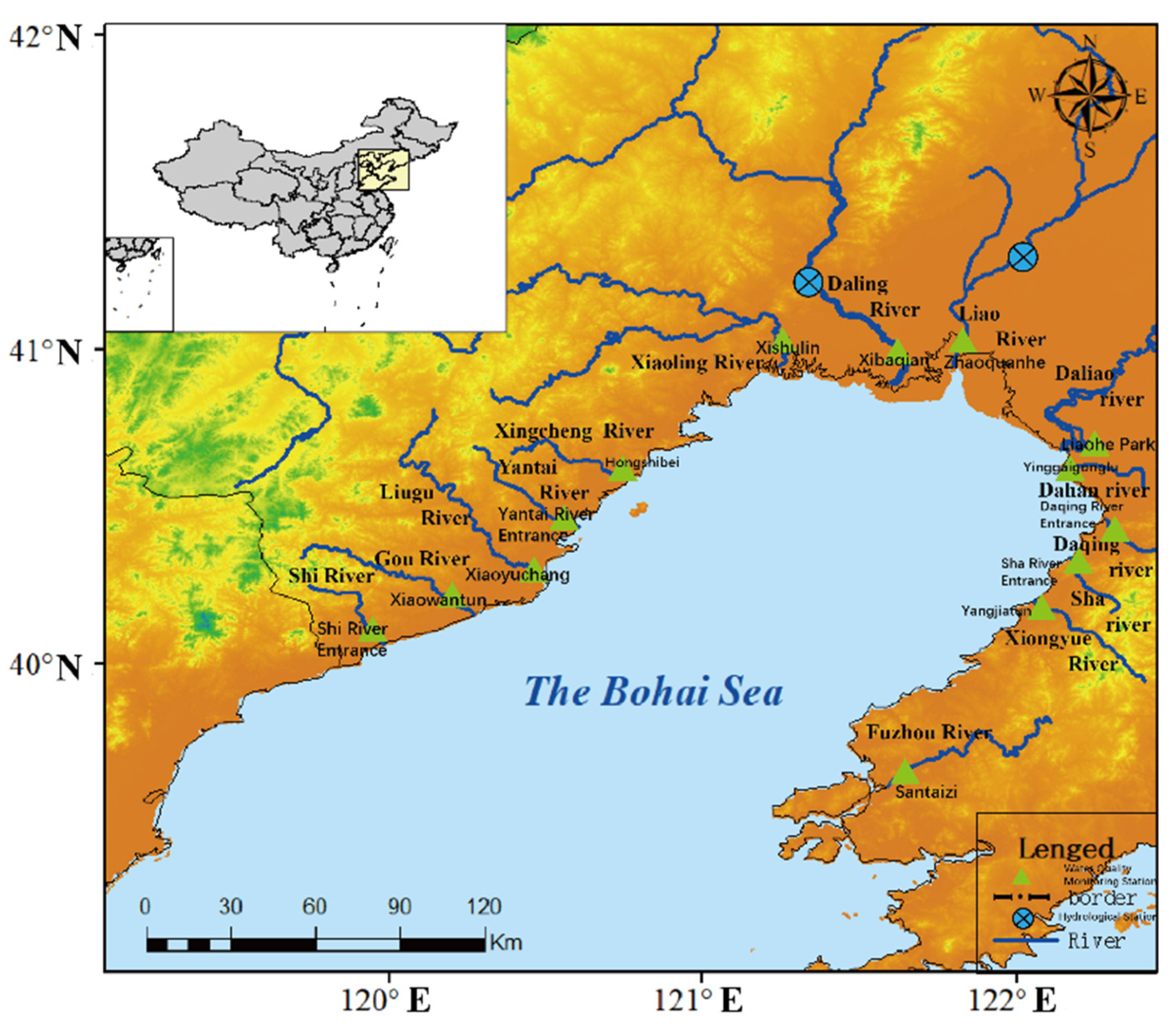
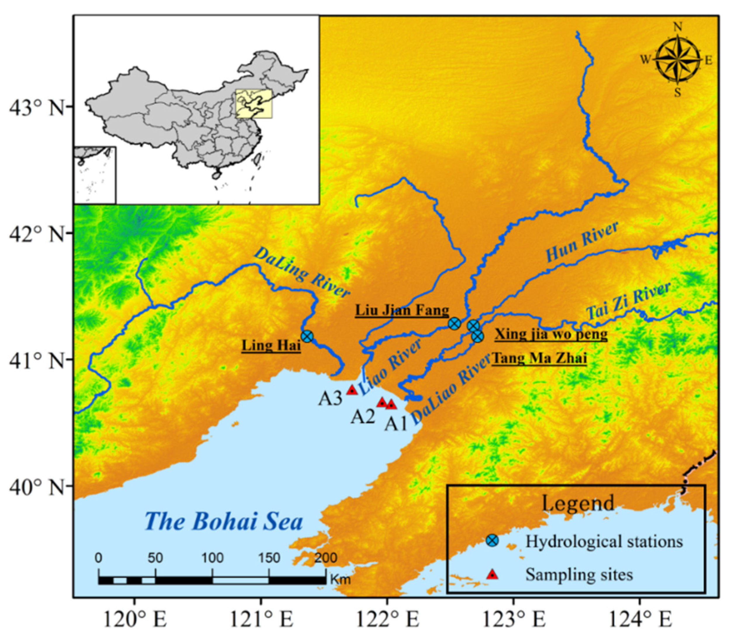
The area of the study was the Bohai sea area and the rivers entering in Liaodong Bay, as shown in Figure 1. The rivers entering into the Liaodong Bay include Daliao (Upstream is Hun and Taizi Rivers), Liao Daling, Xiaoling, Xingcheng, Yantai, Liugu, Dog, Shi, Dali, Daqing, Sha, Xiongyue, and Fuzhou Rivers [37]. Among the above rivers, Daliao, Liao, and Daling Rivers have an average annual runoff of more than 1 billion m³. Daliao River has a watershed area of 26,556 km², a total length of 470 km, and an average annual runoff of 4.76 billion m³; the watershed area of Liao River is 219,000 km², with a total length of 1396 km and an average multiyear runoff of 3.54 billion m³; the total length of Daling River is 447 km, with a basin area of 23,263 km² and an average multiyear runoff of 1.26 billion m³. We selected sea-entry rivers in the Liaodong Bay region, including Daliao, Liao, and Daling Rivers [38].

3.2. Sample Collection

The COD content of rivers entering the Liaodong Bay area was calculated using actual monitoring data in 2018. The potassium dichromate method was utilized for the determination of COD.

Table 1. Data of 14 rivers that enter Liaodong Bay.

	Rivers	Flow (m3/s)	Monitoring Section	Detected Concentrations of COD (mg/L)
1	Daling River	40	Xibaqian	23.4
2	Daliao River	151	Liaohe Park	13.56
3	Liao River	112.3	Zhaoquanhe	18.8
4	Xiaoling River	14.4	Xishulin	42.25
5	Xingcheng River	5	Hongshibei	0.5
6	Yantai River	5	Yantai River Entrance	0.5
7	Liugu River	18.8	Xiaoyuchang	0.17
8	Gou River	4	Xiaowantun	0.5
9	Shi River	3	Shi River Entrance	0.5
10	Dahan River	5.2	Yinggaigonglu	22.58
11	Daqing River	2	Daqing River Entrance	21.67
12	Sha River	3	Sha River Entrance	19.91
13	Xiongyue River	2	Yangjiatun	14.58
14	Fuzhou River	7.4	Santaizi	20.58

shows the multiyear average flow of rivers in Liaodong Bay and the measured amounts of COD in 2018.

3.3. Model Input

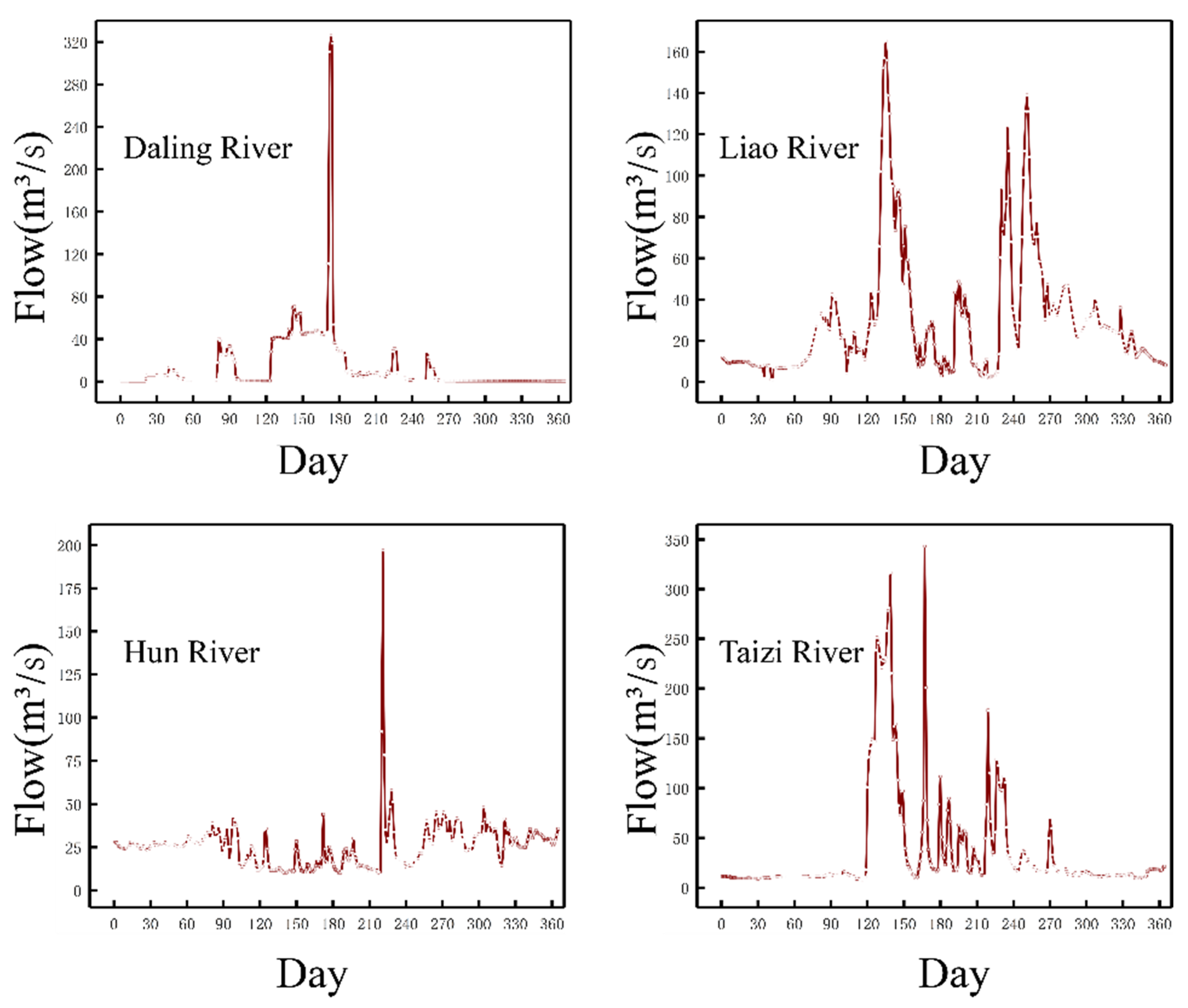
The model river’s topography data were based on genuine big cross-section data: 55 cross-sections of Daliao and Hun Rivers, nine cross-sections of Taizi River, 67 cross-sections of Liao and Liao Rivers, and 48 cross-sections of Daling River. The river flow and water depth statistics were based on genuine hydrological station measurements from 2018. The flow velocity of rivers is shown in Figure 2. Nautical chart data were used to create water region topography. The initial value of water depth was taken as 0 for the 1D river model calculation. Moreover, the initial head was used as that for the model calculation after the head was stabilized. The starting tide level and flow velocity for the sea region were set to 0 m and 0 m/s, respectively. The tide level and flow velocity after the model computation were set as the initial conditions.

A 1D (river) and 2D (sea) linked hydrodynamic water quality model was employed in this investigation. The lower sections of Daling, Liao, and Daliao Rivers were selected by the 1D non-constant flow calculation model of the river channel. Daling River was selected by the river mouth to Linghai hydrological station with a length of 60.6 km. Liao River was selected as the hydrological station from the mouth of the river to Liujianfang on the Liao River, with a length of 106.7 km. Daliao River was selected as two river sections, one from the mouth of the river to Xingjiawopu hydrological station on the Hun River, with a length of 151 km, and the other from the mouth of the river to Tangmazhai hydrological station on the Prince Edward River, with a length of 142.1 km. Due to a lack of significant cross-sectional data, the 11 other rivers, such as Xiaoling River, were incorporated into the model as point source contamination. The whole Bohai Marine was the research region for 2D modeling, and the Liaodong Bay sea area was the center of study and topography encryption.

3.4. Model Setup and Calibration

Linghai hydrological station for Daling River, Liujianfang hydrological station for Liao River, Xingjiawopu hydrological station for Hun River, and Tangmazhai hydrological station for Taizi River were the beginning locations for the 1D river model. The 1D river channel model was created using the daily average flow of the aforementioned five rivers in 2018 as the inflow conditions for computation. The flow boundary established a link between the 1D river cross-section and the 2D sea cross-section. The breadth of the 1D river and its connection defined the node number of the 2D region, and the matching criteria of water depth and flow had to meet at the connection point. Flow boundaries and flow distribution accorded with Manning’s formula on 1D and 2D connection cross-sections [39]. The 2D model of the sea domain first calculated the unstructured grid in planar dimensions by the Euler–Lagrange theorem, and then solved the discrete diving equations by using the unstructured volume method [40,41,42]. Numerical simulation was performed to calculate the flow process of tidal currents [43]. The 2D model was created using the chart’s elevation points and closed polylines to establish the border extent. Unstructured triangular meshes were horizontally selected. The model edge points were diluted once to confirm mesh production and cell scale quality. The model’s grid scale was 4000 m, and the grid in Liaodong Bay was encrypted. The local encryption grid scale was 200 m, based on the computer processing efficiency and model accuracy.

River roughness was calculated using data from the river hydrological station’s measured runoff and water depth. Daliao and Liao Rivers had a roughness of around 0.025, whereas Daling River had a roughness of about 0.045. River roughness was compared with relevant literature and was essentially chosen fairly. The near-shore sea had a rate roughness of approximately 0.016. We considered the effect of organic matter attenuation on the simulation results. We calibrated the attenuation parameters through the measured water quality data from 2014 to 2017, and selected the comprehensive attenuation coefficient of COD as 0.006, so as to minimize the uncertainty of the simulation results and the measured results.

4. Results

4.1. Model Validation

(1)

Validation of the 1D hydrodynamic model for river channel

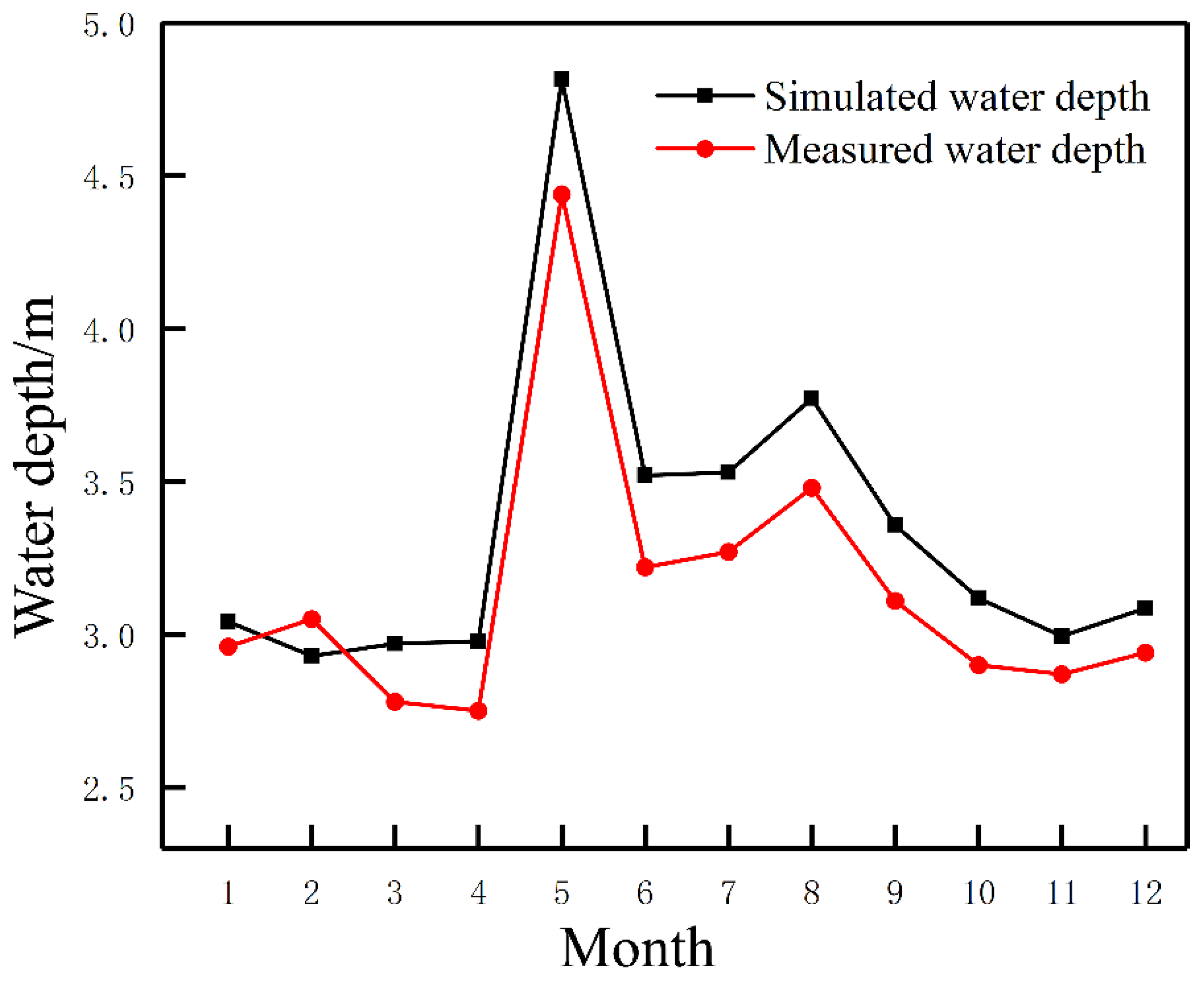
The simulation period was from 1 January 2018 to 31 December 2018, and 8760 h of flow and water depth processes were simulated and computed. We could collect statistics on water depth, flow rate, and water depth at different points of each node when the simulation was over. Tangmazhai hydrological station (120°43′, 41°11′) on Taizi River was chosen for 1D river model validation, and the simulation validation results of water depth are given in Figure 3.

To assess the measured and simulated values for the river 1D non-constant flow validation, three approaches were selected: root mean square error (RMSE), mean relative error (MRE), and R² simulation superiority. The evaluation results are displayed in

Table 2. Calculated water depth evaluation in the cross-section of Tangmazhai.

Month	Simulated Water Level (m)	Measured Water Level (m)	RMSE (m)	MRE (%)	R2
1	3.042	2.960	0.082	0.028	0.999
2	2.930	3.050	0.120	0.039	0.998
3	2.970	2.780	0.190	0.068	0.995
4	2.978	2.750	0.228	0.083	0.994
5	4.816	4.440	0.376	0.085	0.993
6	3.520	3.220	0.300	0.093	0.991
7	3.531	3.270	0.261	0.080	0.994
8	3.772	3.480	0.292	0.084	0.994
9	3.358	3.110	0.248	0.080	0.995
10	3.118	2.900	0.218	0.075	0.994
11	2.995	2.870	0.125	0.043	0.998
12	3.085	2.940	0.145	0.049	0.998

. The simulated water depth variation pattern in each month of the year was consistent with the real data, with R² more than 0.99 in each month, MRE between 0.028% and 0.093%, and RMSE between 0.082 and 0.376, indicating few errors and good fit.

(2)

Validation of the 2D sea hydrodynamic model

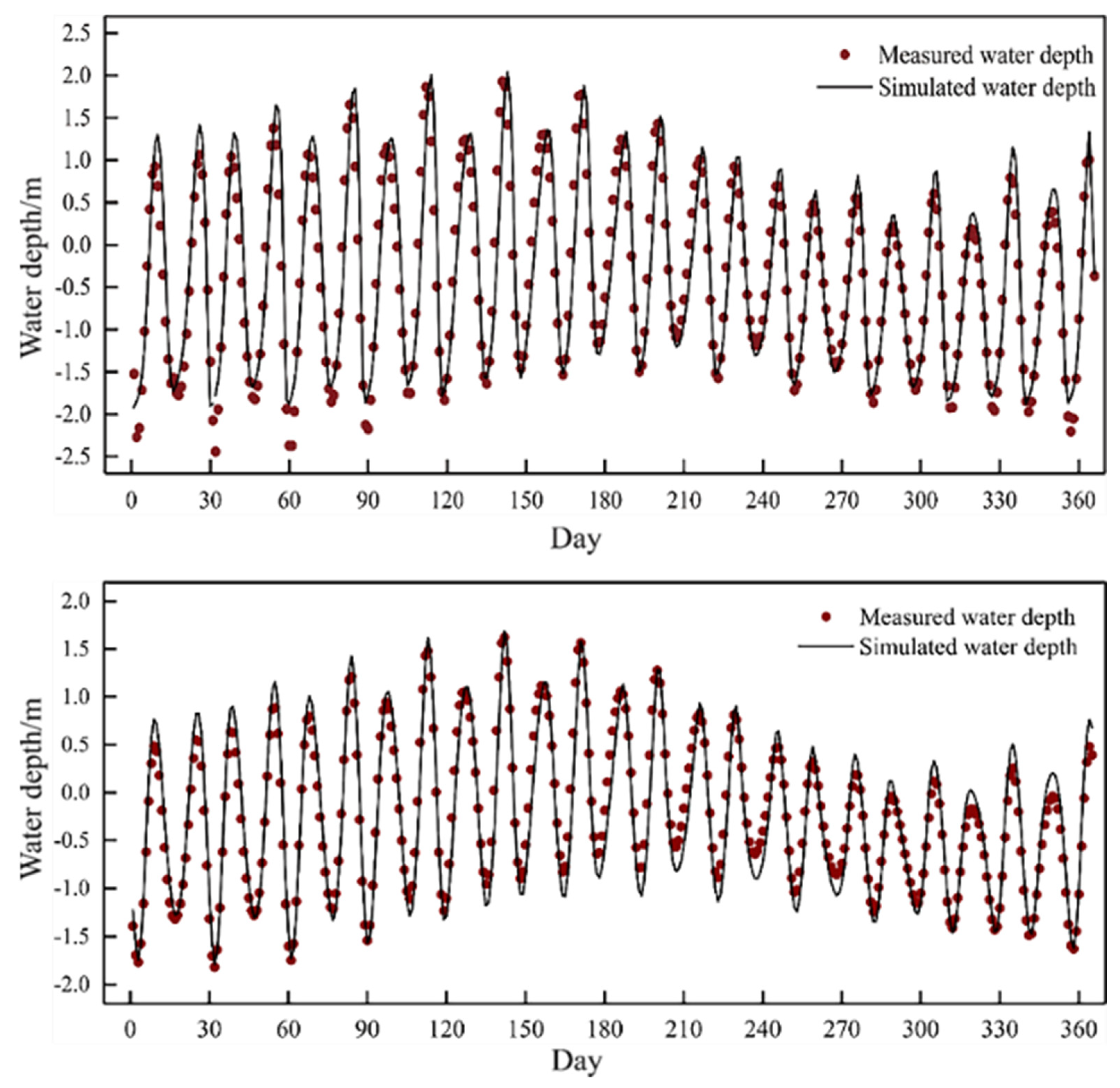
For the sea simulation validation, two tide stations, Huludao and Yingkou, were chosen. The validation results are given in Figure 4, where the solid line represents the simulated tide level and the scattered dots represent the actual observed tide levels.

Wilmott’s skill approach was used for the validation assessment of the 2D non-constant flow in the sea domain [44], and the skill equation is as follows:

$$\mathrm{Skill}=1-\frac{{{\displaystyle \sum }}_{i=1}^N|M-D{|}^2}{{{\displaystyle \sum }}_{i=1}^n{(|M-\overline{D}|+|D-\overline{D}|)}^2},$$

(10)

where M represents the calculated value; D represents the measured value; and $\overline{\mathrm{D}}$ represents the measured mean. The skill value shows the correlation between the deviation of the measured value and the measured mean, including the deviation of the model computed value and the measured mean. Skill evaluation is separated into six categories, with 1 being total agreement between simulation and real measurement, 0.65–1 being excellent, 0.5–0.65 being excellent, 0.2–0.5 being good, 0–0.2 being poor, and 0 being utterly incompatible. The tidal level is simulated for 365 days a year, with 329 days (90.1%) reaching very excellent, very good, and good and with 306 days (83.8%) being very good; 14 days being very good; and nine days being good.

(3)

Validation of the water quality model in the sea

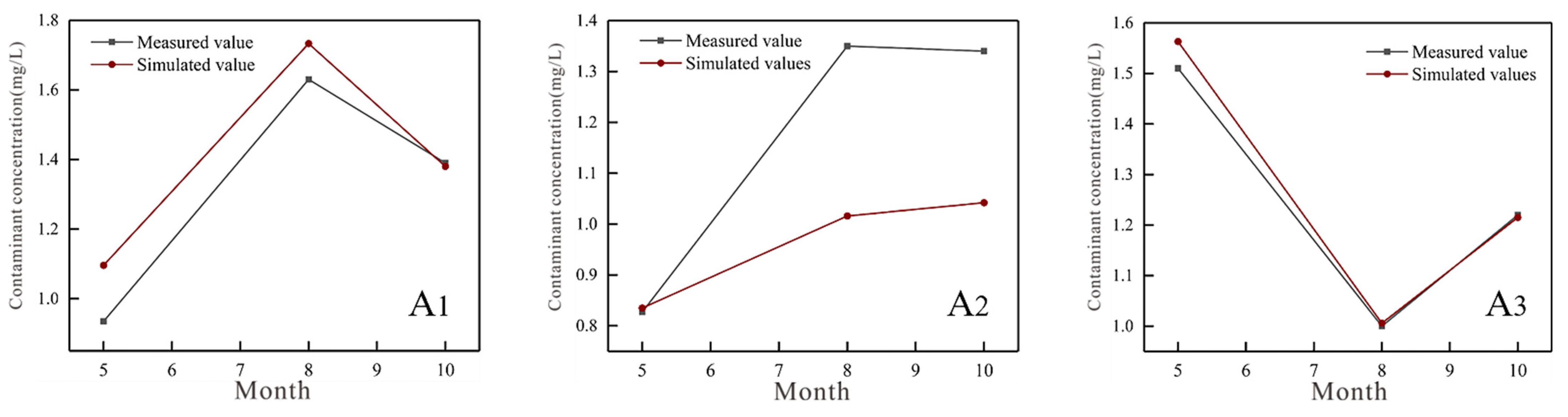
Marine COD was measured three times a year, in spring (May), summer (August), and autumn (October). The study simulated the transport propagation of COD in Liaodong Bay from 1 January 2018 to 31 December 2018. The locations of the real and simulated measurements are illustrated in Figure 5; the simulation and real validation results are displayed in Figure 6, respectively. Wilmott’s skill approach was also adopted for the validation evaluation of the marine pollution transport model, which compared measured and simulated values [45]. The evaluation result of point A1 in August and October was excellent, and May and the whole year was inconsistent; point A2 in May and the whole year was excellent, and August and October was inconsistent; point A3 in May, August, and the whole year was excellent, and October was inconsistent. The following were the main causes of the errors: the model calculated the monthly average of COD, whereas actual monitoring is COD concentration at a specific time; the model calculated the vertical average concentration, whereas actual monitoring is COD concentration at a specific water depth. In addition, the lack of discharge data from some industrial enterprises that discharge directly into the sea, including the influence of COD pollution sources outside Liaodong Bay, were factors.

4.2. Effects of Major Inlet Rivers on COD in Liaodong Bay

The study simulated the seaward process of COD in major rivers, such as Daliao, Liao, and Daling Rivers, from 1 January 2018 to 31 December 2018 [46], the distribution in Liaodong Bay, the influence range, and the change of pollutant concentration in different sea areas.

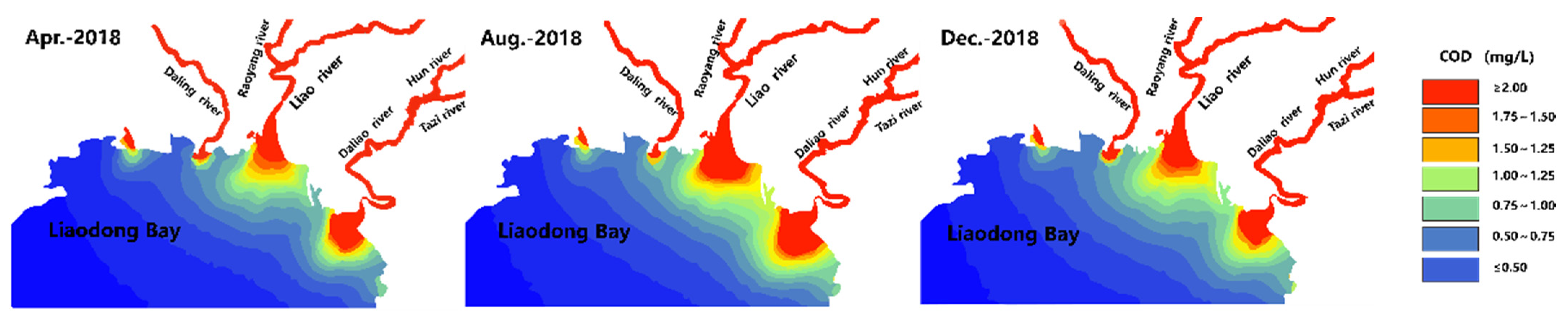
It also stimulated and estimated COD contamination in the Liaodong Bay marine region by major inlet rivers under runoff circumstances in spring (April), summer (August), and winter (December) of 2018. According to the simulation, the influence of pollutants from the main rivers to the sea on the water quality of Liaodong Bay was greatest in summer (August), covering 391.88 km²; the influence range was similar in spring and winter, covering 258.86 km² in spring (April) and 257.89 km² in winter (December).

Table 3. Major rivers into the sea corresponding to the sea COD more than the Class I sea water quality standard range.

	Daling River (km2)	Liao River (km2)	Daliao Rive (km2)	Total (km2)
April	10.79	126.84	121.23	258.86
August	11.12	191.72	189.04	391.88
December	10.48	129.89	117.52	257.89

and Figure 7 illustrate the distribution of marine regions in Liaodong Bay with COD values surpassing the Class I seawater quality requirement.

The simulated water quality (in terms of COD) in Liaodong Bay in summer 2018 (August) was 139.81 km² for Class II, 73.55 km² for Class III, 62.11 km² for Class IV, and 116.41 km² for poor Class IV. In summer 2018 (August), Daliao River had the highest effect on Liaodong Bay’s water quality with 191.7 km²; Liao River had 189.0 km²; which was similar to Daliao River’s influence, and Daling River haf a lower influence with 11.1 km². The simulated areas of various water quality levels in Liaodong Bay waters in summer (August) are shown in

Table 4. Water quality area (COD) of major rivers entering the sea corresponding to various types of water in Liaodong Bay waters in August 2018.

	Class II (km2)	Class III (km2)	Class IV (km2)	Poor IV (km2)	Total (km2)
Daling River	4.51	1.6	2.21	2.8	11.12
Liao River	53.39	54.6	30.08	50.97	189.04
Daliao River	81.91	17.35	29.82	62.64	191.72
Total	139.81	73.55	62.11	116.41	391.88

* Note: Class II is Class II water quality Sea area. Class III is Class III water quality Sea area. Class IV is Class IV water quality Sea area. Poor IV is Poor IV water quality Sea area.

.

4.3. Sudden Water Pollution Accident Simulation Study

Water pollution incidents have occurred in recent years [47], and the Liaodong Bay region has yet to build an emergency water pollution accident warning system [48,49]. In this study, the selected pollutant to be leaked in a water pollution accident was a substance containing zinc, and the transport process of the pollutant in the main inlet rivers, the time of reaching the inlet, the time of reaching the maximum concentration of the pollutant in the inlet, the time of reaching the maximum influence range of the pollution mass, and the time of returning the inlet to Class I water quality when the sudden water pollution event occurred in Daliao, Liao, and Daling Rivers were simulated.

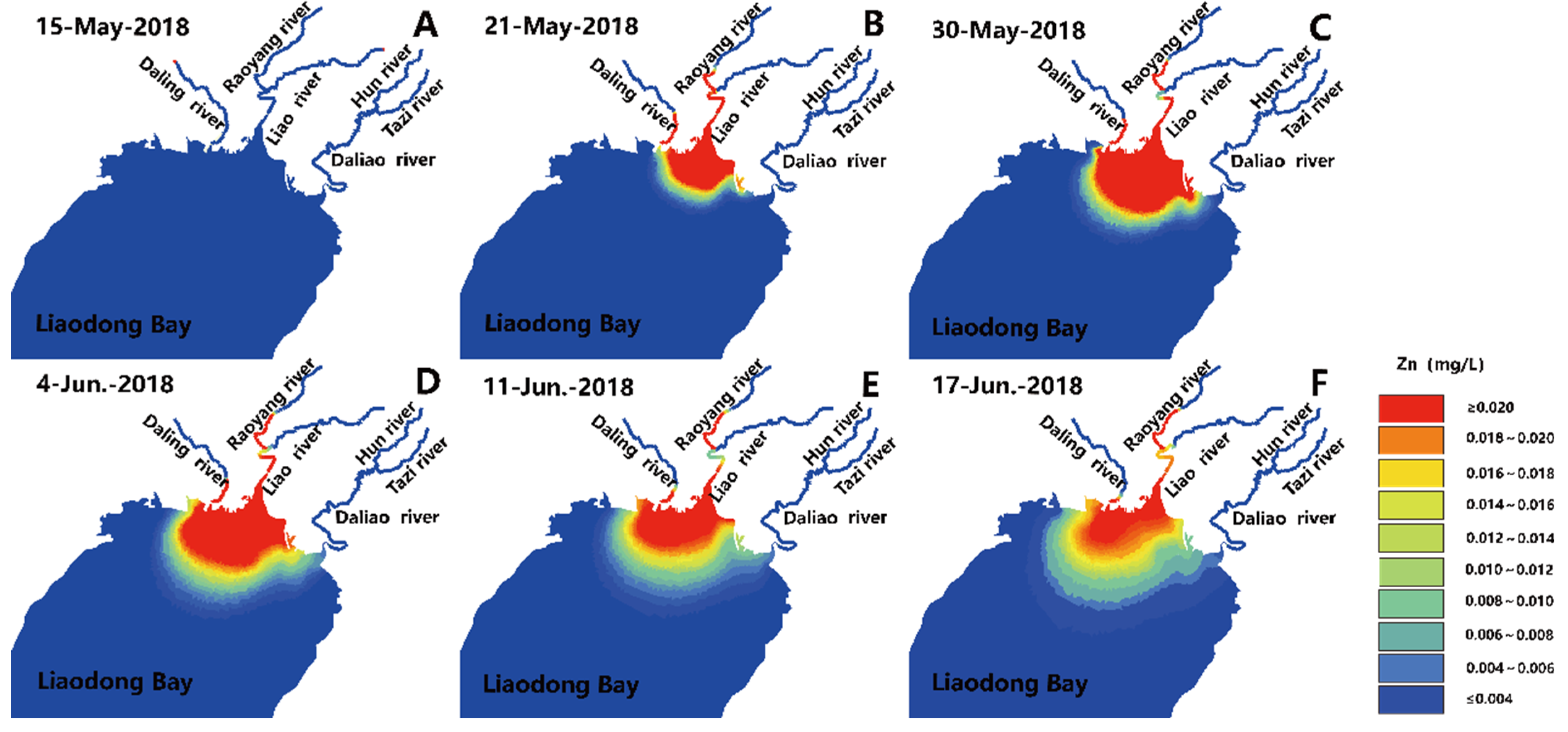
If a spill of zinc-containing pollutants occurred at the Daling River Linghai station section on 15 May 2018, assuming that the peak pollutant concentration at the Daling River Linghai station was 20 mg/L, then, according to the simulation results, after 60.6 km of river transport, the front of the pollutant mass would reach the sea inlet on 21 May (day 7), the maximum pollutant concentration would reach the sea inlet on May 30 (day 16), with a maximum value of 1.28 mg/L, the sea pollution range would reach its maximum on 4 June (day 21), and the mouth of the sea pollutant concentration would drop to 0.02 mg/L or less and return to Class I water quality standard on 17 June (day 34). The pollutant transmission and propagation from the Daling River outbreak are illustrated in Figure 8.

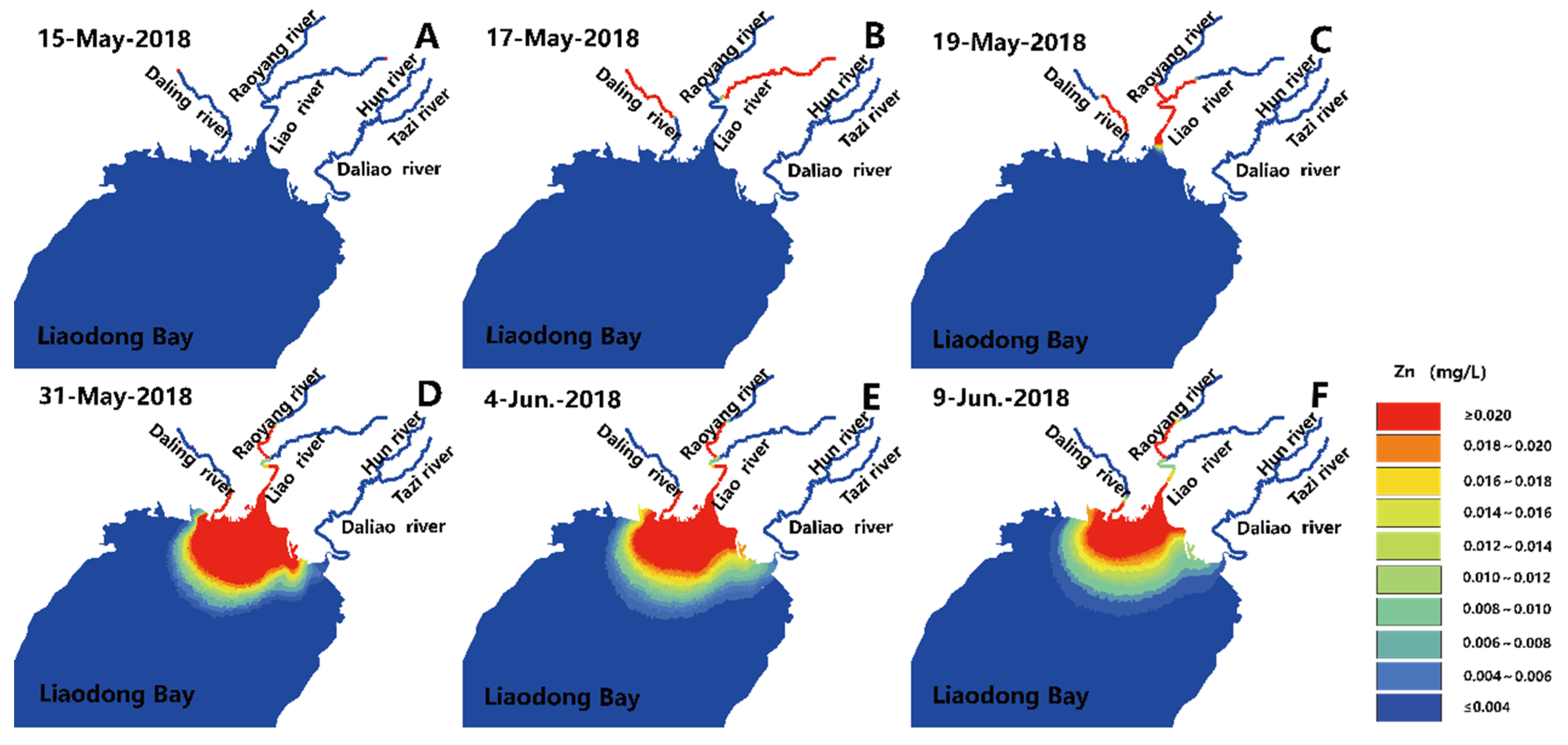
If a sudden leakage of zinc-containing pollutants at the Liusafang hydrological station section of Liao River occurred on 15 May 2018, assuming that the peak pollutant concentration at the Liujianfang hydrological station section was 20 mg/L, then, according to the simulation calculation results, after 106.7 km of river transport, the pollutant front would reach the sea inlet on 17 May (day 3), the pollutant concentration at the sea inlet would reach its maximum on 19 May (day 5), with the maximum value of 4.35 mg/L, the sea pollution range would reach its maximum on 31 May (day 17), the concentration at the mouth of the sea would drop to below 0.02 mg/L and return to Class I water quality standard on June 9 (day 26). The pollutant transportation and propagation in the sudden water pollution accident in Liao River are shown in Figure 9.

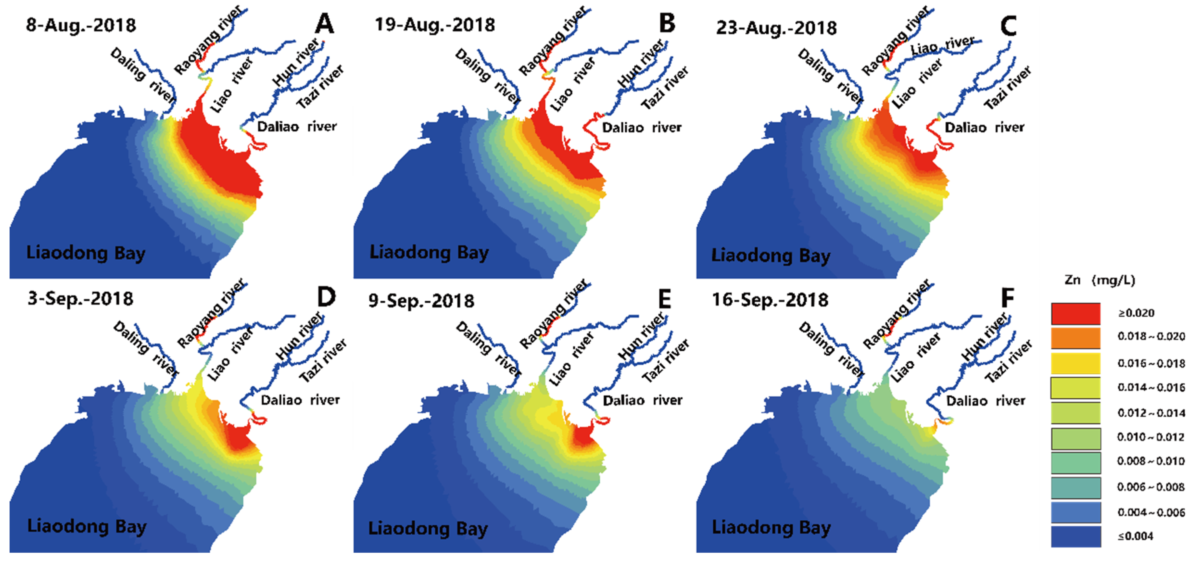
If a sudden leakage of zinc-containing pollutants occurred in Hun River on 8 August 2018 at Xingjiawopu hydrological station, assuming that the maximum concentration of pollutants at Xingjiawopu hydrological station section was 20 mg/L, then, according to the simulation calculation results, after 151 km of river transport, the pollutants would reached the sea inlet on 19 August (day 12), the pollutant concentration at the sea inlet would reach its maximum on 23 August (day 16), with the maximum value of 0.51 mg/L, the pollution range of the sea would reached its maximum on 3 September (day 27), and the pollutant concentration at the mouth of the sea would drop to below 0.02 mg/L and return to Class I water quality standard on 16 September (day 40). The pollutant transmission and propagation from the sudden water pollution accident in Hun River are displayed in Figure 10.

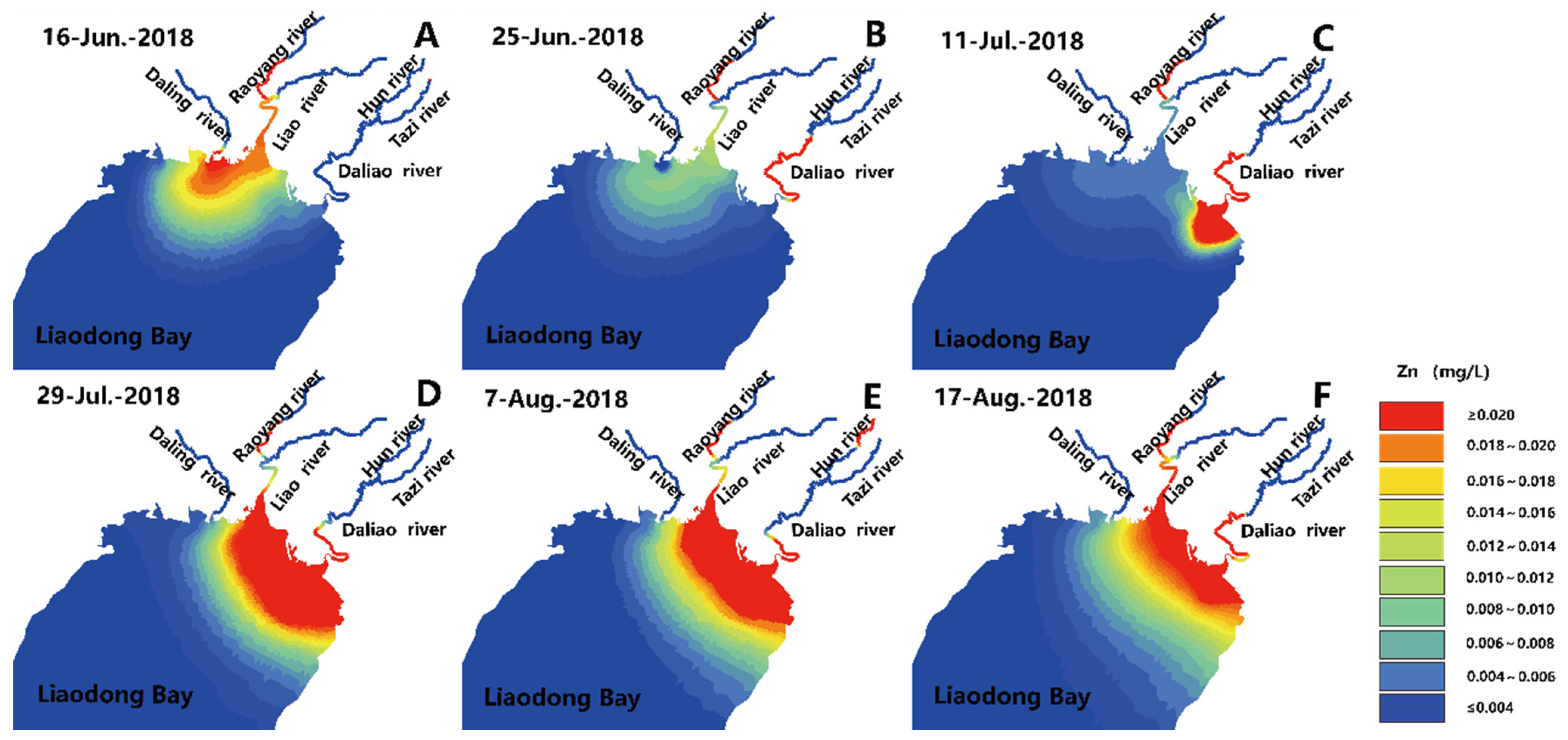
If the zinc pollutant spill occurred in Taizi River on 16 June 2018 at Tangmazhai station section, assuming that the maximum pollutant concentration at Tangmazhai station section was 20 mg/L, according to the simulation calculation results, after 142.1 km of river transport, the pollutant would reach the sea inlet on 25 June (day 10), the pollutant at the sea inlet would reach its maximum on 11 July (day 26), with the maximum value of 4.66 mg/L, the pollution range of the sea would reach its maximum on 29 July (day 44), and the pollutants at the mouth of the inlet would drop to below 0.02 mg/L and return to Class I water quality standard on 17 August (day 63). The pollutant transmission and spread from the sudden water pollution accident in the Taizi River are shown in Figure 11.

The transmission speed of the zinc-containing pollution group in the Liao River was the quickest, following a sudden water pollution event in rivers entering the sea. The pollution group might reach the entrance of the sea and have an influence on it after two days via 106.7 km of river transport. Given that the reaction time to a sudden water pollution incident is limited and the response is tough, we must develop an emergency plan and prepare ahead of time. The pollution mass in the Daling River spread six days after entering the sea, despite the fact that reaction planning time was insufficient. The Hun River had a 151 km river channel with an 11-day transmission propagation time, whereas the Taizi River had a 142 km river channel with a nine-day transmission propagation time. The sudden water pollution event response preparation time was relatively long, and response work was relatively easy.

Following the entry of Zn-containing pollution masses from several rivers entering the sea, the polluted area of the sea reached its maximum after 14 days in the case of Daling River, 15 days for Liao River, 15 days for Hun River, and 34 days for Taizi River. The pollution event timing, the incoming river flow, the pollutant concentration overlaid on each river, and other elements all had roles.

Table 5. Pollutants into the sea, peak present and receding times of the sudden water pollution accident of the river into the sea.

River	Accident Occurred	Time of Arrival	Time of Peak	Restore Class I
Daling River	15 May 2018	21 May 2018	30 May 2018	17 June 2018
Liao River	15 May 2018	17 May 2018	19 May 2018	9 June 2018
Hun River	8 August 2018	19 August 2018	23 August 2018	16 September 2018
Taizi River	16 June 2018	25 June 2018	11 July 2018	17 August 2018

* Note: Accident occurred is the time for pollution accident occurred. Time of arrival is the time of arrival of pollutants in the estuary. Time of peak is the time of peak pollution concentration in the estuary. Restore Class I is the time for the estuary to restore Class I water quality.

shows various water pollution episodes in rivers that led to marine pollution, including peak present and retreating times.

5. Conclusions

This study built a hydrodynamic deriving pollutant transport model of Liaodong Bay area and its main inlet rivers. It concluded that in summer (August), the main inlet rivers carried COD to the bay in an area of 392 km², including 140 km² of Class II water quality, 74 km² of Class III, 62 km² of Class IV, and 116 km² of poor Class IV. The influence range on the sea area in April (spring) and December (winter) was relatively small, about 258 km² (water quality below Class II). The influence range of Daliao River on the water quality of Liaodong Bay in August (summer) was 191.7 km² (water quality below Class II). The influence range of Liao River was 189.0 km² (water quality below Class II), which was close to the influence range of Daliao River. The influence range of Daling River was small, at 11.1 km² (water quality below Class II). When a sudden water pollution accident containing zinc pollutants in rivers entering the sea occurred at the Liujianfang section of Liao River, the pollutants arrived at the mouth of the sea on day 3, which was the shortest time. The preparation work for the accident was short and difficult. When it occurred at the Xingjiawopu section of Hun River, pollutants entered the sea on day 12. If the accident occurred at the Tangmazhai section of Prince Edward River, pollutants entered the sea on day 10. The pollutant transmission and propagation time in Hun River and Prince Edward River exceeded 10 days, and the preparation work for the accident was relatively adequate. When the pollution occurred at Linghai section of Daling River, the pollutants entered the sea on day 7. The preparation time for accident response was longer than that of Liao River and shorter than that of Hun and Prince Rivers. The six-day work was also tight for emergency preparation. This study fills the gap in the research on the response to sudden water pollution incidents in Liaodong Bay waters and major inlet rivers. It also has important reference value and guidance for pollution management.

References

- Qiao, Y.; Feng, J.; Cui, S.; Zhu, L. Long-term changes in nutrients, chlorophyll a and their relationships in a semi-enclosed eutrophic ecosystem, Bohai Bay, China. Mar. Pollut. Bull. 2017, 117, 222–228. [Google Scholar] [CrossRef] [PubMed]
- Nixon, S.W. Coastal marine eutrophication: A definition, social causes, and future concerns. Ophelia 1995, 41, 199–219. [Google Scholar] [CrossRef]
- Smith, V.H.; Tilman, G.D.; Nekola, J.C. Eutrophication: Impacts of excess nutrient inputs on freshwater, marine, and terrestrial ecosystems. Environ. Pollut. 1999, 100, 179–196. [Google Scholar] [CrossRef]
- Heisler, J.; Glibert, P.M.; Burkholder, J.M.; Anderson, D.M.; Cochlan, W.; Dennison, W.C.; Dortch, Q.; Gobler, C.J.; Heil, C.A.; Humphries, E.; et al. Eutrophication and harmful algal blooms: A scientific consensus. Harmful Algae 2008, 8, 3–13. [Google Scholar] [CrossRef] [PubMed] [Green Version]
- Mao, X.; Kuang, C.; Gu, J.; Kolditz, O.; Chen, K.; Zhang, J.; Zhang, W.; Zhang, Y. Analysis of chlorophyll-a correlation to determine nutrient limitations in the Coastal Waters of the Bohai Sea, China. J. Coast. Res. 2017, 33, 396–407. [Google Scholar] [CrossRef]
- Hao, Z.; Xu, H.; Feng, Z.; Zhang, C.; Zhou, X.; Wang, Z.; Zheng, J.; Zou, X. Spatial distribution, deposition flux, and environmental impact of typical persistent organic pollutants in surficial sediments in the Eastern China Marginal Seas (ECMSs). J. Hazard. Mater. 2021, 407, 124343. [Google Scholar] [CrossRef] [PubMed]
- Steele, J.H. A comparison of terrestrial and marine ecological systems. Nature 1985, 313, 355–358. [Google Scholar] [CrossRef]
- Xin, M.; Wang, B.; Xie, L.; Sun, X.; Wei, Q.; Liang, S.; Chen, K. Long-term changes in nutrient regimes and their ecological effects in the Bohai Sea, China. Mar. Pollut. Bull. 2019, 146, 562–573. [Google Scholar] [CrossRef]
- Yin, Y.; Zhang, Y.; Liu, X.; Zhu, G.; Qin, B.; Shi, Z.; Fen, L. Temporal and spatial variations of chemical oxygen demand in Lake Taihu, China, from 2005 to 2009. Hydrobiologia 2011, 665, 129–141. [Google Scholar] [CrossRef]
- Vigiak, O.; Grizzetti, B.; Udias-Moinelo, A.; Michela, Z.; Chiara, D.; Fayçal, B.; Alberto, P. Predicting biochemical oxygen demand in European freshwater bodies. Sci. Total Environ. 2019, 666, 1089–1105. [Google Scholar] [CrossRef]
- Liang, J.; Liu, J.; Xu, G.; Chen, B. Distribution and transport of heavy metals in surface sediments of the Zhejiang nearshore area, East China Sea: Sedimentary environmental effects. Mar. Pollut. Bull. 2019, 146, 542–551. [Google Scholar] [CrossRef] [PubMed]
- Romanou, A.; Chassignet, E.P.; Sturges, W. Gulf of Mexico circulation within a high-resolution numerical simulation of the North Atlantic Ocean. J. Geophys. Res. Oceans. 2004, 109, C01003. [Google Scholar] [CrossRef]
- Guerzoni, S.; Frignani, M.; Giordani, P.; Frascari, F. Heavy metals in sediments from different environments of a Northern Adriatic Sea area, Italy. Econ. Environ. Geol. 1984, 6, 111–119. [Google Scholar] [CrossRef]
- Xu, B.; Yang, X.; Gu, Z.; Zhang, Y.; Chen, Y.; Lv, Y. The trend and extent of heavy metal accumulation over last one hundred years in the Liaodong Bay, China. Chemosphere 2009, 75, 442–446. [Google Scholar] [CrossRef] [PubMed]
- Feng, H.; Jiang, H.; Gao, W.; Weinstein Michael, P.; Zhang, Q.; Zhang, W.; Yu, L.; Yuan, D.; Tao, J. Metal contamination in sediments of the western Bohai Bay and adjacent estuaries, China. J. Environ. Manage. 2011, 92, 1185–1197. [Google Scholar] [CrossRef] [PubMed]
- Bu, H.; Song, X.; Zhang, Y. Using multivariate statistical analyses to identify and evaluate the main sources of contamination in a polluted river near to the Liaodong Bay in Northeast China. Environ. Pollut. 2019, 245, 1058–1070. [Google Scholar] [CrossRef]
- Stynes, M. Steady-state convection-diffusion problems. Acta Numer. 2005, 14, 445–508. [Google Scholar] [CrossRef]
- Borthwick, A.; Barber, R. River and reservoir flow modelling using the transformed shallow water equations. Int. J. Numer. Methods Fluids 1992, 14, 1193–1217. [Google Scholar] [CrossRef]
- Yeung, R.W. Numerical methods in free-surface flows. Annu. Rev. Fluid Mech. 1982, 14, 395–442. [Google Scholar] [CrossRef]
- Ming, P.; Duan, W. Numerical simulation of sloshing in rectangular tank with VOF based on unstructured grids. J. Hydrodynam B 2010, 22, 856–864. [Google Scholar] [CrossRef]
- Szymkiewicz, R. Finite-element method for the solution of the Saint Venant equations in an open channel network. J. Hydrol. 1991, 122, 275–287. [Google Scholar] [CrossRef]
- Molls, T.; Molls, F. Space-time conservation method applied to Saint Venant equations. ISH J. Hydraul. Eng. 1998, 124, 501–508. [Google Scholar] [CrossRef]
- Perthame, B.; Simeoni, C. A kinetic scheme for the Saint-Venant system¶ with a source term. Calcolo 2001, 38, 201–231. [Google Scholar] [CrossRef]
- Yamazaki, D.; De Almeida, G.A.M.; Bates, P.D. Improving computational efficiency in global river models by implementing the local inertial flow equation and a vector-based river network map. Water Resour. Res. 2013, 49, 7221–7235. [Google Scholar] [CrossRef]
- Choi, H.; Moin, P. Effects of the computational time step on numerical solutions of turbulent flow. J. Comput. Phys. 1994, 113, 1–4. [Google Scholar] [CrossRef]
- Weare, T.J. Instability in tidal flow computational schemes. J. Hydraul. Eng. 1976, 102, 569–580. [Google Scholar] [CrossRef]
- Shafroth, P.B.; Wilcox, A.C.; Lytle, D.A.; Hickey, J.T.; Andersen, D.C.; Beauchamp, V.B.; Hautzinger, A.; Mcmullen, L.E.; Warner, A. Ecosystem effects of environmental flows: Modelling and experimental floods in a dryland river. Freshw. Biol. 2010, 55, 68–85. [Google Scholar] [CrossRef]
- Anastasiou, K.; Chan, C. Solution of the 2D shallow water equations using the finite volume method on unstructured triangular meshes. Int. J. Numer. Methods Fluids 1997, 24, 1225–1245. [Google Scholar] [CrossRef]
- Namin, M.; Lin, B.; Falconer, R.A. Modelling estuarine and coastal flows using an unstructured triangular finite volume algorithm. Adv. Water Resour. 2004, 27, 1179–1197. [Google Scholar] [CrossRef]
- Alcrudo, F.; Garcia-Navarro, P. A high-resolution Godunov-type scheme in finite volumes for the 2D shallow-water equations. Int. J. Numer. Methods Fluids 1993, 16, 489–505. [Google Scholar] [CrossRef]
- Cea, L.; French, J.; Vázquez-Cendón, M. Numerical modelling of tidal flows in complex estuaries including turbulence: An unstructured finite volume solver and experimental validation. Int. J. Numer. Methods Eng. 2006, 67, 1909–1932. [Google Scholar] [CrossRef]
- Stansby, P.K. Semi-implicit finite volume shallow-water flow and solute transport solver with k–ε turbulence model. Int. J. Numer. Methods Fluids 1997, 25, 285–313. [Google Scholar] [CrossRef]
- Kim, C.; Lee, J. A three-dimensional PC-based hydrodynamic model using an ADI scheme. Coast. Eng. 1994, 23, 271–287. [Google Scholar] [CrossRef]
- Casulli, V.; Cattani, E. Stability, accuracy and efficiency of a semi-implicit method for three-dimensional shallow water flow. Comput. Math. Appl. 1994, 27, 99–112. [Google Scholar] [CrossRef] [Green Version]
- Abualtayef, M.; Kuroiwa, M.; Tanaka, K.; Matsubara, Y.; Nakahira, J. Three-dimensional hydrostatic modeling of a bay coastal area. J. Mar. Sci. Technol. 2008, 13, 40–49. [Google Scholar] [CrossRef]
- Wang, K. Characterization of circulation and salinity change in Galveston Bay. J. Eng. Mech. 1994, 120, 557–579. [Google Scholar] [CrossRef]
- Dou, Y.; Li, J.; Zhao, J.; Wei, H.; Yang, S.; Bai, F.; Zhan, D.; Ding, X.; Wang, L. Clay mineral distributions in surface sediments of the Liaodong Bay, Bohai Sea and surrounding river sediments: Sources and transport patterns. Cont. Shelf Res. 2014, 73, 72–82. [Google Scholar] [CrossRef]
- Tan, L.; He, M.; Men, B.; Lin, C. Distribution and sources of organochlorine pesticides in water and sediments from Daliao River estuary of Liaodong Bay, Bohai Sea (China). Estuar. Coast. Shelf Sci. 2009, 84, 119–127. [Google Scholar] [CrossRef]
- Engel, B.; Storm, D.; White, M.; Arnold, J.; Arabi, M. A hydrologic/water quality model Applicati11. J. Am. Water Resour. Assoc. 2007, 43, 1223–1236. [Google Scholar] [CrossRef]
- Ewen, J.; Parkin, G.; O’connell, P.E. SHETRAN: Distributed river basin flow and transport modeling system. J. Hydrol. Eng. 2000, 5, 250–258. [Google Scholar] [CrossRef]
- Li, C.; Wu, W.; Yin, Y. Hierarchical elimination selection method of dendritic river network generalization. PLoS ONE 2018, 13, e0208101. [Google Scholar] [CrossRef] [PubMed]
- Madsen, N.K. Divergence preserving discrete surface integral methods for maxwell’s curl equations using non-orthogonal unstructured grids. J. Comput. Phys. 1995, 119, 34–45. [Google Scholar] [CrossRef] [Green Version]
- Ai, T.; Liu, Y.; Huang, Y. The hierarchical watershed partitioning and generalization of river network. Acta Geod. Et Cartogr. Sin. 2007, 36, 231–236. [Google Scholar]
- Willmott, C.J. On the validation of models. Phys. Geogr. 1981, 2, 184–194. [Google Scholar] [CrossRef]
- Qu, L.; Yao, D.; Cong, P. Inorganic nitrogen and phosphate and potential eutrophication assessment in Liaodong Bay. Huan Jing Ke Xue 2006, 27, 263–267. [Google Scholar]
- Xia, K.; Guo, J.; Han, Z.; Dong, M.; Xu, Y. Analysis of the scientific and technological innovation efficiency and regional differences of the land–sea coordination in China’s coastal areas. Ocean Coast. Manag. 2019, 172, 157–165. [Google Scholar] [CrossRef]
- Wu, X.; Hu, J.; Jia, A.; Peng, H.; Wu, S.; Dong, Z. Determination and occurrence of retinoic acids and their 4-oxo metabolites in Liaodong Bay, China, and its adjacent rivers. Environ. Toxicol. Chem. 2010, 29, 2491–2497. [Google Scholar] [CrossRef]
- Meng, W.; Qin, Y.; Zheng, B.; Zhang, L. Heavy metal pollution in Tianjin Bohai bay, China. J. Environ. Stud. 2008, 20, 814–819. [Google Scholar] [CrossRef]
- Guo, B.; Jiao, D.; Wang, J.; Lei, K.; Lin, C. Trophic transfer of toxic elements in the estuarine invertebrate and fish food web of Daliao River, Liaodong Bay, China. Mar. Pollut. Bull. 2016, 113, 258–265. [Google Scholar] [CrossRef]
Figure 1.
Study area and location.
Figure 2.
The flow velocity of rivers.
Figure 3.
Calculated and observed water depth of Tangmazhai station.
Figure 4.
Actual and calculated tide level at Huludao and Yingkou.
Figure 5.
Illustration of Liaodong Bay’s water quality measuring locations.
Figure 6.
Measured and simulated situations of sea area points A1, A2 and A3.
Figure 7.
Water quality distribution of seawater with COD concentration exceeding Class I in April, August, and December 2018.
Figure 8.
Daling River outbreak water pollution accident pollutant transport spread.
Figure 9.
Pollutant transmission and propagation in the sudden water pollution accident in Liao River.
Figure 10.
Hun River outbreak of water pollution accident pollutant transport spread.
Figure 11.
Sudden water pollution accident in the Taizi River pollutant transport spread.