
Calibrating a Hydrological Model in an Ungauged Mountain Basin with the Budyko Framework


1
Flood Control Guarantee and Rural Water Conservancy Center of Guangdong Province, Guangzhou 510635, China
2
Center for Water Resources and Environment, Sun Yat-sen University, Guangzhou 510275, China
3
School of Hydrology and Water Resources, Nanjing University of Information Science and Technology, Nanjing 210044, China
*
Authors to whom correspondence should be addressed.
Water 2022, 14(19), 3112; https://doi.org/10.3390/w14193112
Submission received: 29 August 2022
/
Revised: 27 September 2022
/
Accepted: 28 September 2022
/
Published: 2 October 2022
(This article belongs to the Special Issue Challenges of Hydrological Drought Monitoring and Prediction)
Abstract
:Calibrating spatially distributed hydrological models in ungauged mountain basins is complicated due to the paucity of information and the uncertainty in representing the physical characteristics of a drainage area. In this study, an innovative method is proposed that incorporates the Budyko framework and water balance equation derived water yield (WYLD) in the calibration of the Soil and Water Assessment Tool (SWAT) with a monthly temporal resolution. The impact of vegetation dynamics (i.e., vegetation coverage) on Budyko curve shape parameter ω was considered to improve the Budyko calibration. The proposed approach is applied to the upstream Lancang-Mekong River (UL-MR), which is an ungauged mountain basin and among the world’s most important transboundary rivers. We compared the differences in SWAT model results between the different calibration approaches using percent bias (PBIAS), coefficient of determination (R2), and Nash–Sutcliffe efficiency (NSE) coefficient. The results demonstrated that the Budyko calibration approach exhibited a significant improvement against an unfitted priori parameter run (the non-calibration case) though it did not perform as good as fitting of the calibration by the observed streamflow. The NSE value increased by 44.59% (from 0.46 to 0.83), the R2 value increased by 2.30% (from 0.87 to 0.89) and the PBIAS value decreased by 55.67% (from 39.7 to 17.6) during the validation period at the drainage outlet (Changdu) station. The outcomes of the analysis confirm the potential of the proposed Budyko calibration approach for runoff predictions in ungauged mountain basins.
1. Introduction
The plateau mountain basins are the birthplaces of the world’s large rivers, known as the world water tower [1,2]. The hydrologic conditions of the mountain basins has a direct impact on the supply of water resources, socio-economic development, and environmental changes in the downstream areas [3]. Under changing climatic conditions, significant changes are occurring in the water resources of the mountain basins, which affects the sustainable development of the downstream economy and society [4]. However, the plateau mountain basins have very few hydrological stations. The accurate simulation of the hydrological process in mountain ungauged basins plays an important role in water resource prediction and management [5,6,7,8].
Hydrological information is critical for coping with natural disasters and managing water resources. Hydrological models can provide information, but the traditional calibration method requires hydrological data, which are usually of low quality or unavailable in mountain basins (such as the Tibetan Plateau, Appalachian Plateau and Edwards Plateau) [9,10,11]. Therefore, hydrologists have been looking for various new calibration procedures and data assimilation methods to improve the accuracy of water resource management and prediction in mountain basins without data [12,13].
Over the last decades, several authors have proposed methods to improve the determination of parameters in ungauged mountain basins [14]. Currently, a common approach is parameter regionalization, which means that key parameter values of ungauged regions are inferred from those of gauged basins based on spatial proximity [15,16,17], physical similarity [18,19], and regression [20,21]. However, these regionalization methods depend on the availability of gauged basins and are affected by the uncertainty of the hydrological model structure and a poor understanding of watershed spatial heterogeneity. On the other hand, due to the latest development of remote sensing technology, many attempts have been made to combine multi-source satellite remote sensing data with quasi-globally available topographic data to improve the model performance [22]. Using remote sensing data to estimate various parameters such as evapotranspiration [23], surface soil moisture [24], total water storage [25], river hydraulic geometry parameters [26], snow and ice cover [27], leaf area index (LAI) [28] and normalized difference vegetation index (NDVI) [29] provides additional an input for model configuration, model calibration and data assimilation.
Budyko postulated that precipitation and potential evapotranspiration are the two main variables controlling the long-term average water balance. The Budyko framework is considered to be one of the most important frameworks linking climatic conditions with runoff and actual evapotranspiration in the catchment area [30], and has been successfully used to study the interaction between hydrological processes, climate variability and landscape characteristics [31]. The Budyko framework can be considered as a lumped model, providing a fast first-order estimate of the distribution of precipitation partitioning into evaporation and runoff. The model is simple and has low input requirements compared to complex hydrological models such as the semi-distributed or fully distributed model [32]. In addition to the first-order estimation of evaporation, the Budyko framework is used to study the sensitivity of runoff to changes in climate variables and catchment characteristics, to investigate the impact of climate change on the hydrological response of the catchment, to understand the long-term availability of water resources management, determines water volume, and separates the effects of natural climate variability and direct human activity on changes in annual mean runoff [32,33,34,35]. A series of empirical formulas have been developed for the Budyko curve based on theoretical research and a case study of regional water balance over the past 50 years. Among them, the Fu [33,34] equation has been widely used. In addition, the controlling parameter ω (in the Fu equation) is linearly correlated [35]. Burek used the Budyko framework to calibrate the Community water model (CWATM) of unmeasured basins in the world, instead of conducting calibrations using several stations with existing data of unmeasured basins and trying to regionalize the results [36]. However, a default Budyko curve shape parameter (ω = 2.6) was used for all stations without considering that there existed differences in the vegetation and climate seasonality index. Actually, these characteristics have a significant effect on the controlling parameter ω [37,38,39,40]. In addition, there was an obvious Budyko-type relationship between precipitation, potential evaporation, and actual evapotranspiration in each basin for the annual scale. i.e., the annual scale and shape parameter ω are different in different regions [41]. Therefore, the Budyko framework for calibrating the CWATM did not significantly improve the simulation performance in some catchments due to the fact that the variation in Budyko curve shape parameter ω was not considered [36], and the CWATM was mainly applied to the assessment of the water supply and human and environmental water demands. Hence, we attempt to calibrate a physically based hydrological model using the Budyko framework with consideration of the impact of vegetation dynamics (i.e., vegetation coverage) on the Budyko curve shape parameter ω to improve its calibration.
Over the last decades, quantitative hydrological models have become useful tools for water resource management [42]. Reliable hydrological models are important, especially in data-scarce watersheds [43]. Conceptual hydrological models are parsimonious and can achieve accurate simulation after calibration with the observed discharge [44]. In contrast, physically based distributed hydrological models are better at representing spatial variability and can produce more reliable results when describing water cycle processes [44]. In these models, the semi-distributed hydrological model soil and water assessment tool (SWAT) has been widely used to simulate hydrological processes at the basin scale [45]. The SWAT is a conceptual physically based hydrological model which was developed for water resource management, soil erosion, and water quality; it has also been used to assess the impacts of land management practices, and climate effects on hydrological processes in diverse environmental conditions [46,47,48]. For example, the SWAT model has been used to evaluate the impact of land cover changes on the hydrological processes in rapidly developing catchments [49,50]. Furthermore, the SWAT model has been identified as a successful model for simulating hydrological processes in mountain basins because it can consider the impact of snow, the snowmelt cycle and frozen soil on the hydrological cycle through a strong physical mechanism [51,52,53]. The estimated value of SWAT evapotranspiration was consistent with the estimated value of the Budyko curve [54]. Thus, it is feasible to apply SWAT coupled with the Budyko framework to simulate streamflow in the mountain basins.
Therefore, the purpose of this study is to provide a new calibration approach by integrating the Budyko framework and the water balance equation in complex ungauged mountain basins, i.e., by combining the Budyko framework and a hydrological model (SWAT) by considering the variation of parameter ω and applying the model to complex mountain regions that lack hydrometeorological information. We focus on the upstream Lancang-Mekong River (UL-MR) in the Tibetan Plateau, which suffers from data scarcity as demonstrated in many previous studies [55]. The data scarcity motivated us to explore the applicability of the new calibration approaches. The proposed calibration method is unique for the following reasons: (1) precipitation and evaporation are available for all sites, and the Budyko curve parameter ω is calculated by using a simple semi-empirical formula based on Fu’s equation in which the impact of vegetation dynamics (i.e., vegetation coverage) on ω was considered; (2) the results of Budyko calibration are significantly improved compared with those of uncalibrated parameters though it is not as good as the observed water flow calibration.
2. Study Area and Datasets
2.1. Study Area
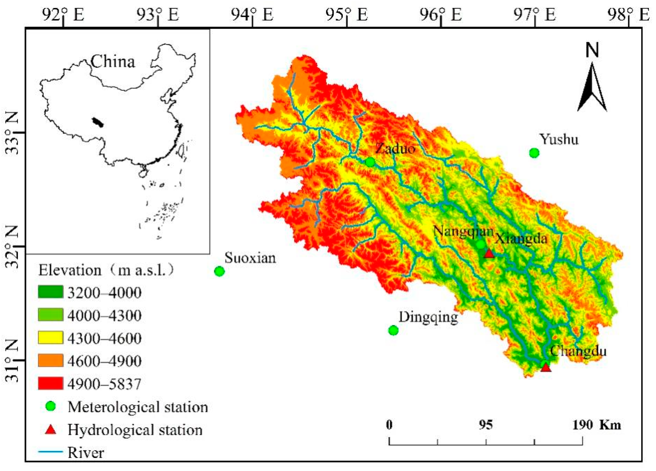
Lancang-Mekong River, the largest cross-border river in Asia, originates from the Guozongmucha Mountain on the Qinghai Tibetan Plateau and flows through the South China Sea through seven climatic zones and six countries (China’s Yunnan Province, Myanmar, Lao, Thailand, Cambodia, and Vietnam) [56,57]. The UL-MR was defined as the catchment area above the Changdu (31°11′ N, 97°11′ E) hydrologic station which covers a drainage area of about 53,720 km2, and is directed to the Zaqu and Angqu rivers in the Qinghai-Tibetan Plateau (Figure 1). It has different topographical conditions and various climatic zones due to the existence of many high mountains and deep valleys in southwestern China. The altitude ranges from approximately 3500 m to 5500 m, which is characterized by a low annual average temperature of −3 °C to 3 °C. Most of the region is cold and dry with a long winter, frequent wind and large temperature difference between day and night. The UL-MR is located in the east of the Qinghai Tibet Plateau and is affected by the East Asian monsoon in summer and by mid-latitude westerlies in winter. The annual precipitation ranges from 400 mm to 700 mm, and 70% of annual rainfall occurs during the wet season (June–September). Direct anthropogenic disturbances are nearly absent in the most remote and least developed areas in southwest China due to the highly rugged terrain, high altitudes, and a particularly cold climate. Moreover, the hydrological stations network is quite sparse in UL-MR due to the harsh environment [55].
2.2. Data
2.2.1. Hydrometeorological Data
The meteorological data (such as daily precipitation, daily maximum temperature, minimum temperature, daily mean wind speed, daily mean relative humidity and solar radiation from 1979 to 2014) were downloaded from the official website of the Meteorological Data Center of the China Meteorological Administration in this study (http://data.cma.cn/, (accessed on 1 May 2021)) (Figure 1). Monthly streamflow data during 1961–2013 for the Xiangda and Changdu hydrological stations were derived from the Qinghai Provincial Bureau of Hydrology and Water Resources Survey (http://water.sanjiangyuan.org.cn, (accessed on 1 May 2021)). Streamflow data were used to calibrate and validate the SWAT model in streamflow simulations. The specific information of hydrometeorological stations is shown in Table 1.
2.2.2. Spatial Data
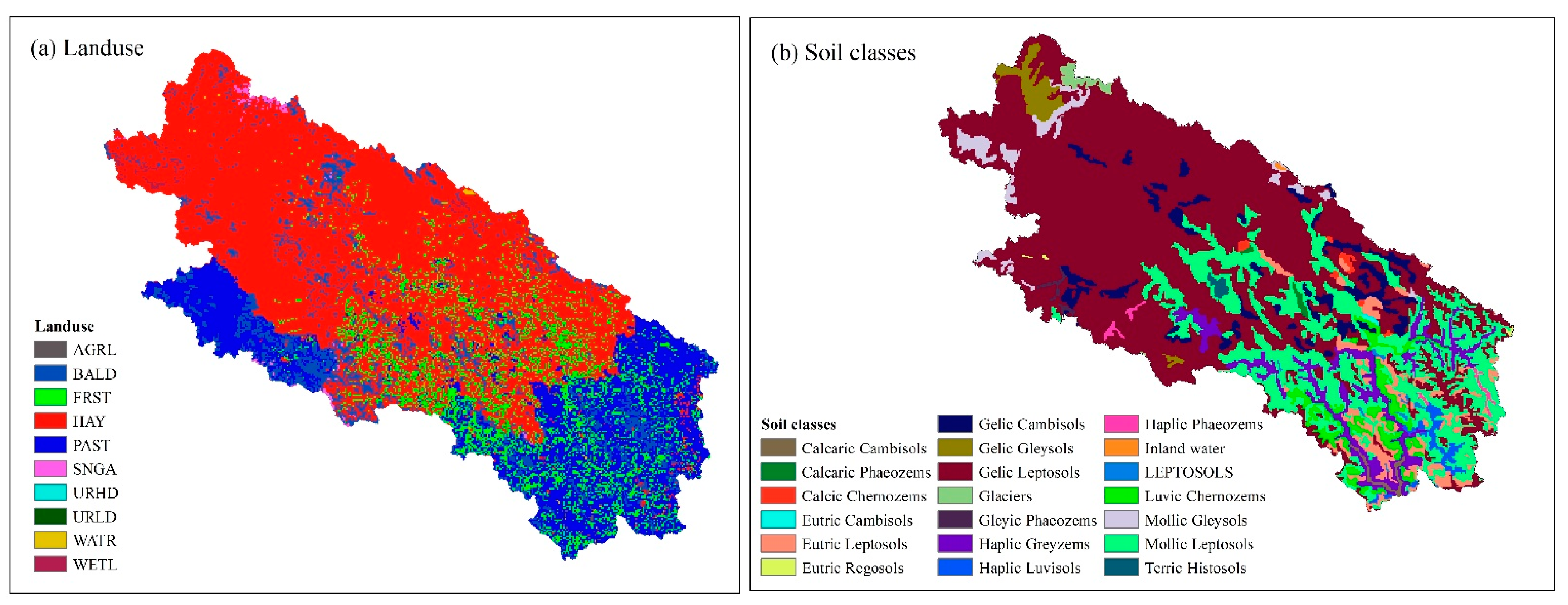
Th land use, soil, terrain and NDVI data used in UL-MR to develop SWAT model are summarized in Table 2. The 2000 LULC map was obtained from a supervised classification of Landsat Thematic Mapper images which were classified as the standard LULC classification of SWAT (Figure 2a). Watershed boundaries and the stream network were extracted from 90 m digital elevation model (DEM) data from the Space Shuttle Radar Terrain Mission (SRTM). The 1:500,000 scale soil map which was developed by the Food and Agriculture Organization (FAO) was downloaded from the website of http://www.fao.org/soils-portal/soil-survey/soil-maps-and-databases/ (accessed on 1 May 2021). This soil data map reflects the distribution and characteristics of the different soil types (Figure 2b). Soil water characteristics such as hydraulic conductivity and effective water capacity are calculated by using the SPAW model. A 10 km NDVI dataset was used to calculate vegetation characteristics for UL-MR which were obtained using the NOAA Advanced Very High Resolution Radiometer sensor [58]. Annual NDVI values of long-term averages (from 1981 to 2006) were obtained from the above datasets.
3. Methodology
The goal of this study is to provide a hydrological model (SWAT) with the data calculated using the Budyko framework for parameter calibration in order to solve the problem of runoff prediction and simulation in ungauged regions. Therefore, the main method is to calibrate the parameters of the SWAT model based on the calculation of the water yield derived from the Budyko framework.
3.1. Budyko Framework
The Budyko framework assumes that the water balance is stable over a long period of time, and changes in water storage in the catchment are negligible [59]. The evapotranspiration (E) is determined by the dynamic water balance in a natural basin as follows:
where P, E, and R represent precipitation, evapotranspiration and runoff, respectively, and ΔS represents the change in terrestrial water storage. When ΔS is negligible in the long-term water balance, the annual mean precipitation (P) is divided into the annual mean actual evapotranspiration (E) and runoff (R). This partitioning is achieved by using the Budyko equation, a simple water balance model (E/P = f (EP/P)), where EP means annual potential evapotranspiration. The model proposed by Fu [33] and popularized by Zhang [34] is widely used and has the following expression:
E = P − R − ΔS
E, EP are the annual average actual evapotranspiration and the annual average potential evapotranspiration, respectively, calculated using the Penman–Monteith equation outlined in FAO-56 [60].
ω is an empirical parameter, which determines the shape of the Budyko curve and reflects the influence of other factors such as climate seasonality and land surface characteristics on water and energy balances. The soil properties and topography are relatively stable, although it will affect the change of water balance in the catchment area. Therefore, vegetation dynamics (such as vegetation coverage) were selected to represent changes in surface conditions. The vegetation coverage (M) was estimated with the following equation, which represents the percentage of total surface area covered by vegetation [35]:
As described in previous studies, NDVImax is the NDVI value of dense green vegetation and NDVImin is the NDVI value of bare soil [35,37]. NDVImax and NDVImin are global constants that are independent of vegetation/soil type, as was demonstrated by Gutman and Ignatov [61]. In our study, we used the NDVImax of dense forest (0.80) and NDVImin of bare soil (0.05), as described in the literature. We use the semi-empirical equation proposed by Li to calculate the empirical parameter ω [37]; this method is only based on remote sensing vegetation information and simple parameterization in a specific basin. It achieved good performance in simulating annual evapotranspiration.
ω = 2.36 × M + 1.16
3.2. Hydrological Data
3.2.1. SWAT Model Setup
The SWAT model was developed by the United States Department of Agriculture (USDA) to simulate the hydrological processes, water quality, and soil erosion of large complex watersheds [62,63,64]. An interface between ArcSWAT 2012 and ArcGIS was used to establish a model in this work. For use in the ArcSWAT 2012, the UL-MR was subdivided into 10 sub-watersheds and the hydrologic response units (HRUs), which is the smallest spatial unit for calculating hydrological processes. HRUs are generated according to the combination of land use, soil type and slope of the sub basin [65]. Two major phases were considered in the hydrological simulation of the SWAT model. For the land phase, the quantity of water loads from the land to the main channel was calculated according to the soil–water balance in the hydrological cycle simulation function of the SWAT model. In this phase, the Soil Conservation Service-Curve Number (SCS-CN) was used for estimating the runoff yield [66]. The movement of these loads through the channel network to the outlet of the watershed was controlled by the routing phase. Manning’s formula was used to define the velocity and rate of channel flow and channel routing was represented by variable storage routing in this study. The Penman–Monteith method was chosen to calculate potential evapotranspiration because it is relatively common and the estimated potential evapotranspiration is more accurate than other calculation methods if there are sufficient weather data such as wind speed, relative humidity, and solar radiation [67].
3.2.2. Calibrating the SWAT Model Based on the Budyko Framework
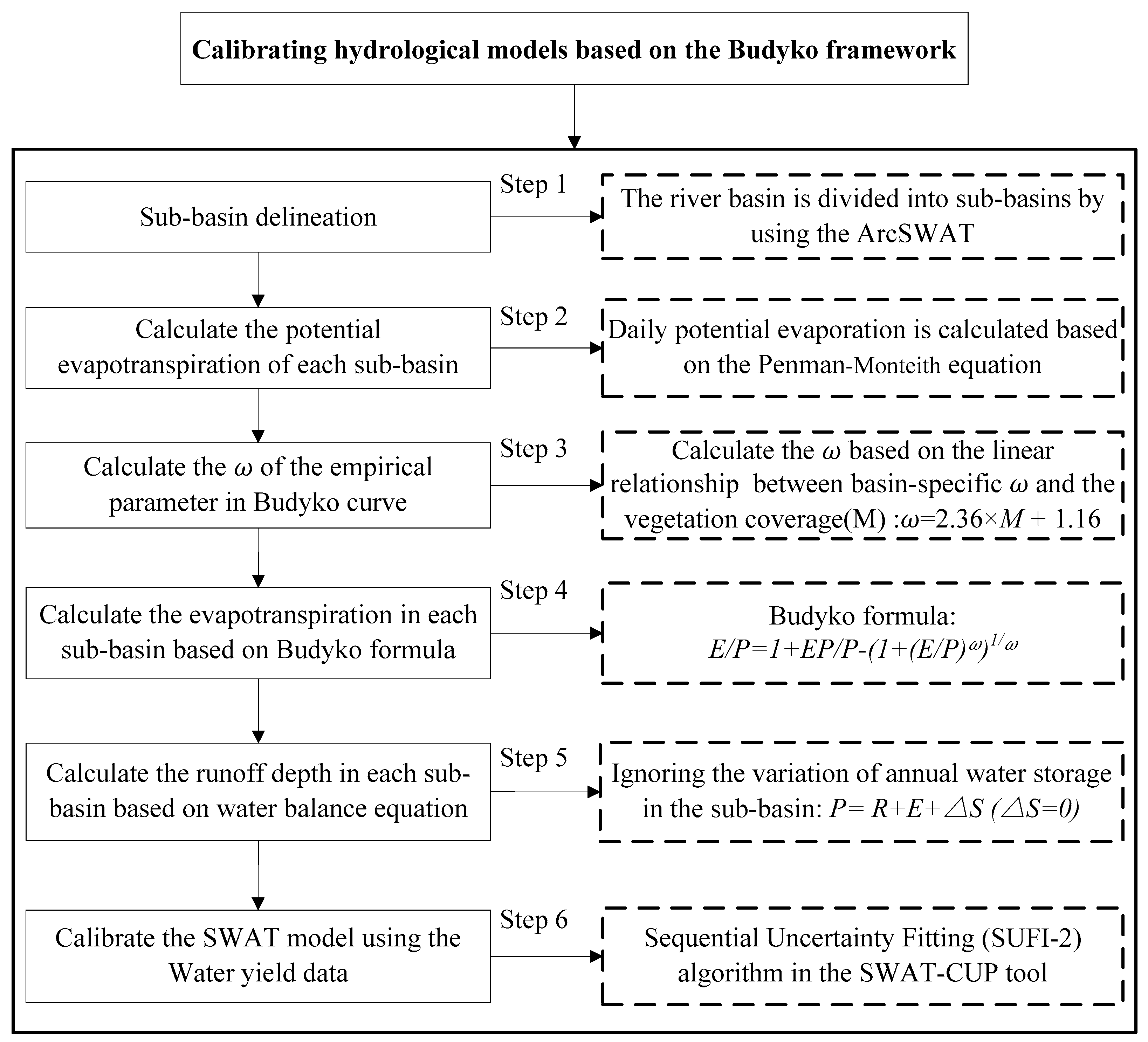
Taking the UL-MR basin as a case study for hydrological modeling of the ungauged basin, the SWAT model was calibrated using water yield data derived from the Budyko framework and water balance equation. Figure 3 briefly describes the schematic diagram of the method. The calibration approach is based on the following two assumptions: (1) the changes in the water storage at the annual scale in the sub-basins are ignored; (2) the objective of the calibration method is to calibrate the hydrological model in the ungauged regions. The calibration method includes the following steps:
Step 1: Delineation of the sub-basins. The river basin is divided into several sub-basins by using the watershed delineation tool in ArcSWAT.
Step 2: Calculation of the potential evapotranspiration of the sub-basins. The daily potential evaporation is calculated using the Penman–Monteith formula. The SWAT model (ArcSWAT interface) automatically assigns the meteorological data to the sub-basins by using the data of one measurement station closest to the centroid of each sub basin [68].
Step 3: Calculation of the empirical parameter ω in the Budyko curve. The suitable linear relationship between the vegetation coverage (M) and the basin-specific ω is calculated by Equation (4).
Step 4: Calculation of the evapotranspiration in each sub-basin based on Fu’s equation (Equation (2)).
Step 5: Calculation of runoff depth in each sub-basin using the water balance formula with an annual scale. The changes in the annual water storage in the sub-basins were ignored and the annual runoff depth of each sub-basin was calculated by using the equation of the annual water balance as follows:
Step 6: Calibration of the SWAT model using the runoff depth data in each sub-basin. The annual runoff depth is roughly equivalent to the annual water yield. We used the annual water yield to calibrate the SWAT model for all sub-basins with an annual scale by using the SUFI-2 algorithm of the SWAT-CUP tool. The SWAT model parameters of each sub-basin obtained from the water yield was used to simulate the monthly discharge during the validation period.
3.2.3. Model Assessment Criteria
We used NSE, PBIAS, and R2 as three general indicators to evaluate the model performance (the 1500 simulations from each SWAT model scenario were compared). The three general indicators are widely used in hydrological simulation, as well as in the evaluation of model simulation effects to study the relationship between climate, environment, soil, ecology and hydrological processes [48,68], and they are defined as follows:
where , , and are measured, simulated average measured and average simulated values in each time step i, and n is the number of data points. This study followed the criteria proposed by Moriasi to evaluate the performance of the model [69].
3.3. Evaluation of the Budyko Calibration
In this study, another two calibration cases for the SWAT model were examined to test whether the Budyko calibration approach (hereafter referred to as the Sim Budyko) was able to optimize the model performance in the UL-MR. The first calibration case involved calibration with runoff data alone (hereafter referred to as the Sim streamflow). In the second calibration case, the SWAT model was used with priori parameters which were not calibrated (hereafter referred to as non-calibration).
The SWAT model was run on a monthly timescale, where the first two years (1959–1960) were considered a warm-up period to eliminate the influence of the initial conditions of model simulation. The period of 1961–1987 served as the calibration period during which the sensitive parameters were calibrated to fit the measured monthly runoff. The remaining period of 1988–2007 was used to validate the simulated flow at the outlet of the watershed (Changdu). The observed streamflow records at Xiangda hydrologic station during 2008–2012 were used for the model validation due to the lack of long-time series flow data.
Automatic calibration of monthly flow simulation was performed using the sequential uncertainty fitting (SUFI-2) algorithm from the SWAT-CUP tool [70]. The sensitivity analysis was performed with a one-at-a-time procedure for sensitive hydrological parameters for the UL-MR. According to previous research [2,62], the thirteen common sensitive hydrological parameters (SURLAG, CN2, ALPHA_BNK, GWQMN, GW_DELAY, GW_REVAP, ESCO, SOL_AMC(1), SOL_BD(1), CH_N2, SOL_K(1), CH_K2, SFTMP, SMTMP, TIMP) were considered and eight parameters (CN2, GW_DELAY, GWQMN, ESCO, SOL_K(1), CH_N2, ALPHA_BNK, SOL_BD(1)) were ultimately determined as highly sensitive parameters (Table 3). The calibration procedures were performed in three iterations, with 500 simulations per iteration (a total of 1500 simulations during calibration) using the NSE coefficient as the objective function [71]. After each iteration, the parameter ranges was updated (usually narrowed) according to the new parameters range suggested by SWAT-CUP and the appropriate physical ranges.
4. Results and Discussion
4.1. The Variability of Parameter ω
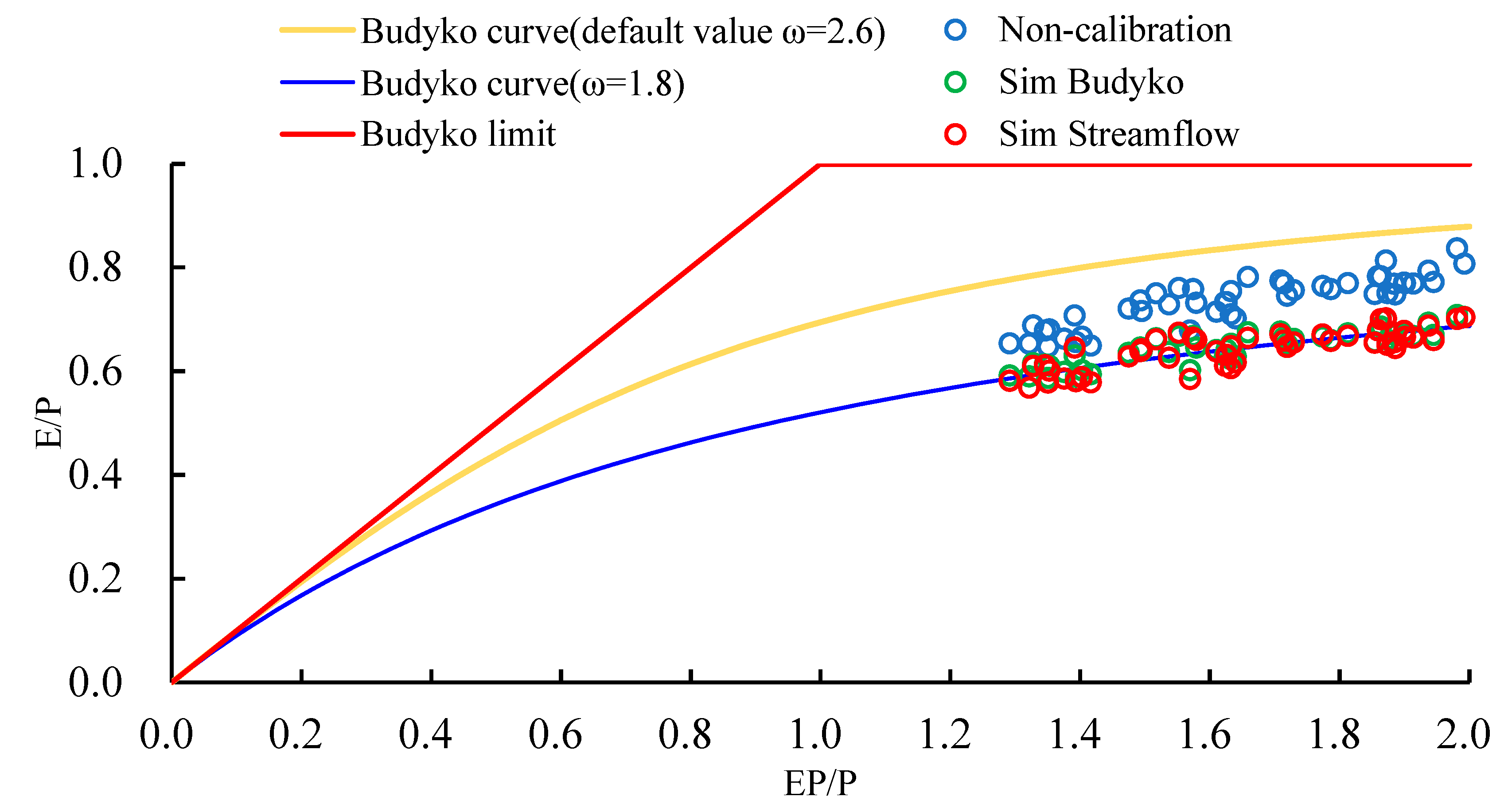
The basin-specific ω value is derived from the simple parameterization equation, as described in Section 3.3 (see also Figure 4). The annual NDVI values of the UL-MR are obtained from the global NDVI dataset and averaged from 1984 to 2012; subsequently, the long-term averaged annual vegetation coverage is calculated using Equation (3). The basin-specific ω value is significantly different from the default value of 2.6 and the fitted ted value of Equation (4) of 1.8. Figure 4 shows the Budyko curves obtained from the different basin-specific ω values. The red dots represent the results of the actual streamflow calibration, the green dots represent the results of the Budyko calibration, and the blue dots represent the results from the non-calibrated SWAT model. It is evident that the red dots and the green dots are close to each other, and they are closely distributed around the Budyko curve (ω = 1.8). The Budyko curve (with the default ω value 2.6) is notably different from the fitted value 1.8. It is obvious that Fu’s expression with the basin-specific ω value, which is calculated using the semi-empirical equation, is able to grasp the interannual variability of the regional energy and water balance among different climate zones.
Burek [36] used the Budyko framework to calibrate a global hydrological model (e.g., CWATM) in ungauged basins and a fixed ω (ω = 2.6) was used to calculate the evapotranspiration values for all basins. However, the curve shape parameter ω in Fu’s formula controls how much water is available for evaporation given the available energy. Previous research revealed that the vegetation and climate zone significantly affect changes in the controlling parameter ω [37]. Hence, the use of the fixed value ω = 2.6 did not provide good results for the Budyko calibration in some regions of the world.
4.2. Streamflow Simulation Performance for Different Calibration Approaches
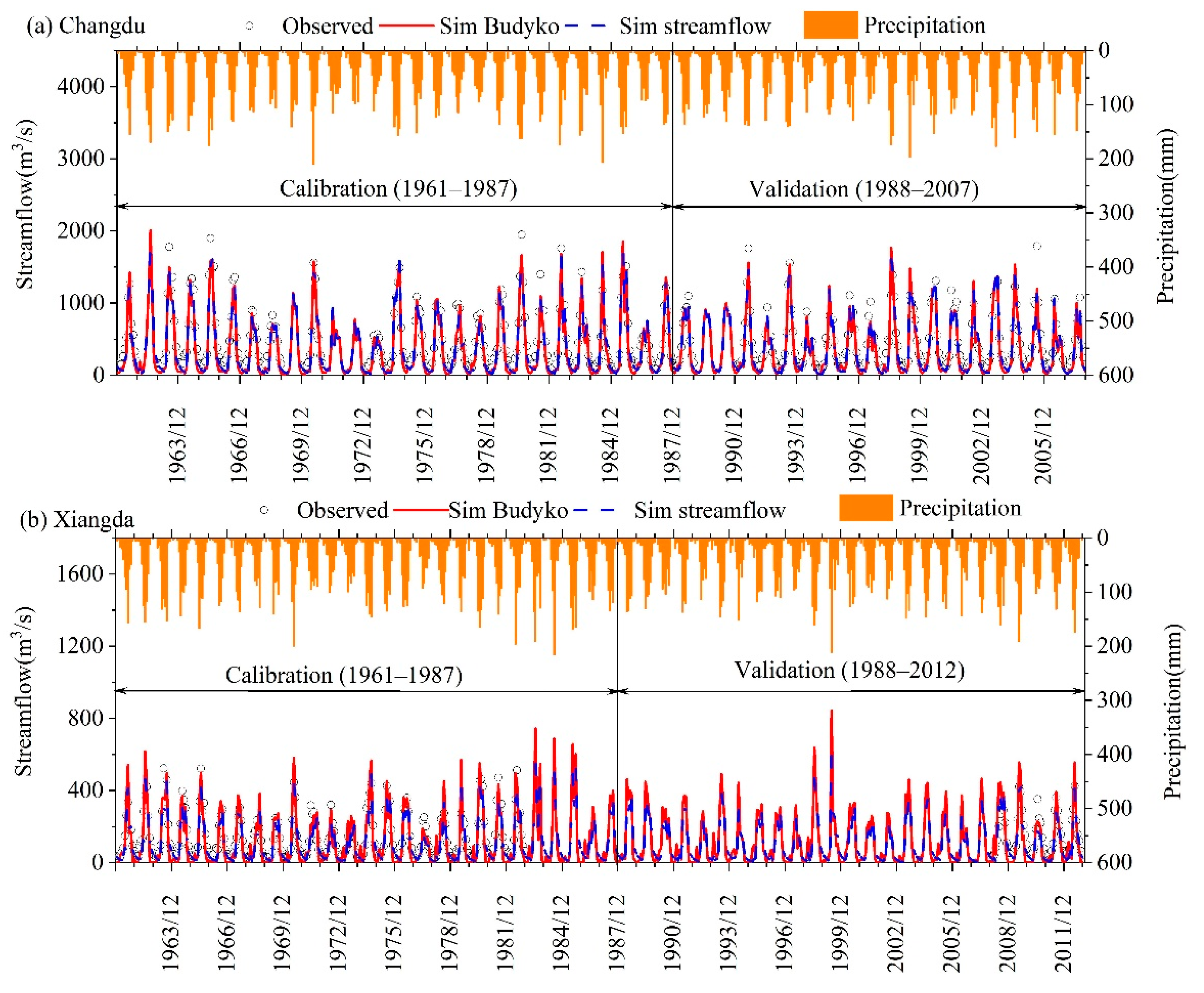
Figure 5 shows the comparison of the measured and simulated monthly streamflow hydrographs obtained from ‘Sim Budyko’ and ‘Sim streamflow’ calibrations with the optimal parameter values. It is observed that the simulated streamflow hydrographs with the ‘Sim streamflow’ calibration exhibited a closer agreement with the observed streamflow hydrographs, whereas the model simulation using the Budyko calibration approach exhibited worse performance and there was a tendency of the SWAT model to underestimate the streamflow in the dry season. It seems that the Budyko calibration approach is well suited for monthly streamflow simulation in this mountain ungauged basin with good precision.
In the calibration period, the ‘Sim streamflow’ calibration achieved very good results at the Changdu station, with an NSE coefficient of 0.88, a PBIAS of 17.69, and an R2 of 0.93. The ‘Sim Budyko’ calibration also produced very good results with an NSE of coefficient 0.84, a PBIAS of 22.38, and an R2 of 0.91. During the validation period, the NSE values were 0.83 (Changdu) and 0.44 (Xiangda) and the calculated relative streamflow errors were 17.6% (Changdu) and 14.78% (Xiangda), respectively. Furthermore, the relatively high R2 values (0.76–0.89) indicated that the ‘Sim Budyko’ approach performs well in explaining the measured flow variation.
Figure 5 also clearly and intuitively shows the difference in the simulation results using the Budyko calibration approach. It can be seen that the simulation results are significantly better than those without calibration; that is, the NSE value increased by 44.59 % (from 0.46 to 0.83), the R2 value increased by 2.30% (from 0.87 to 0.89) and the PBIAS value decreased by 55.67% (from 39.7 to 17.6) during the validation period of Changdu station. Similarly, during the validation period of Xiangda station, the NSE value increased by 29.55 % (from 0.31 to 0.44), the R2 value increased by 26.32% (from 0.56 to 0.76) and the PBIAS value decreased by 68.94% (from 47.87 to 14.87) (Table 4).
Referring to the judgment standard of Moriasi [69], the model was well calibrated and suitable for monthly flow simulation in the study area. However, due to the complexity of natural processes, and due to errors in driving data and runoff observations, it is never possible to obtain a perfect model fit in hydrological modeling [71]. Etter indicated that uncertain streamflow estimates can be useful for model calibration but that the estimates by scientists need to be improved by performing training or more advanced data filtering before they are useful for model calibration [72]. Marco confirmed the potential of a MODIS snow map as additional data to inform hydrological models leading to more reliable and accurate discharge estimates [73]. Bouslihim showed that the quality and resolution of soil data affect all hydrological cycle components, mainly the soil water content and water production, but do not lead to significant differences in runoff simulation, especially after the model calibration [74]. Therefore, the upper benchmark should not be an unrealistic perfect simulation but should take into account potential errors in the data. We encourage further discussions and exploration of the impact of hydroclimatic situations and data quality on a perfect model fit in future research.
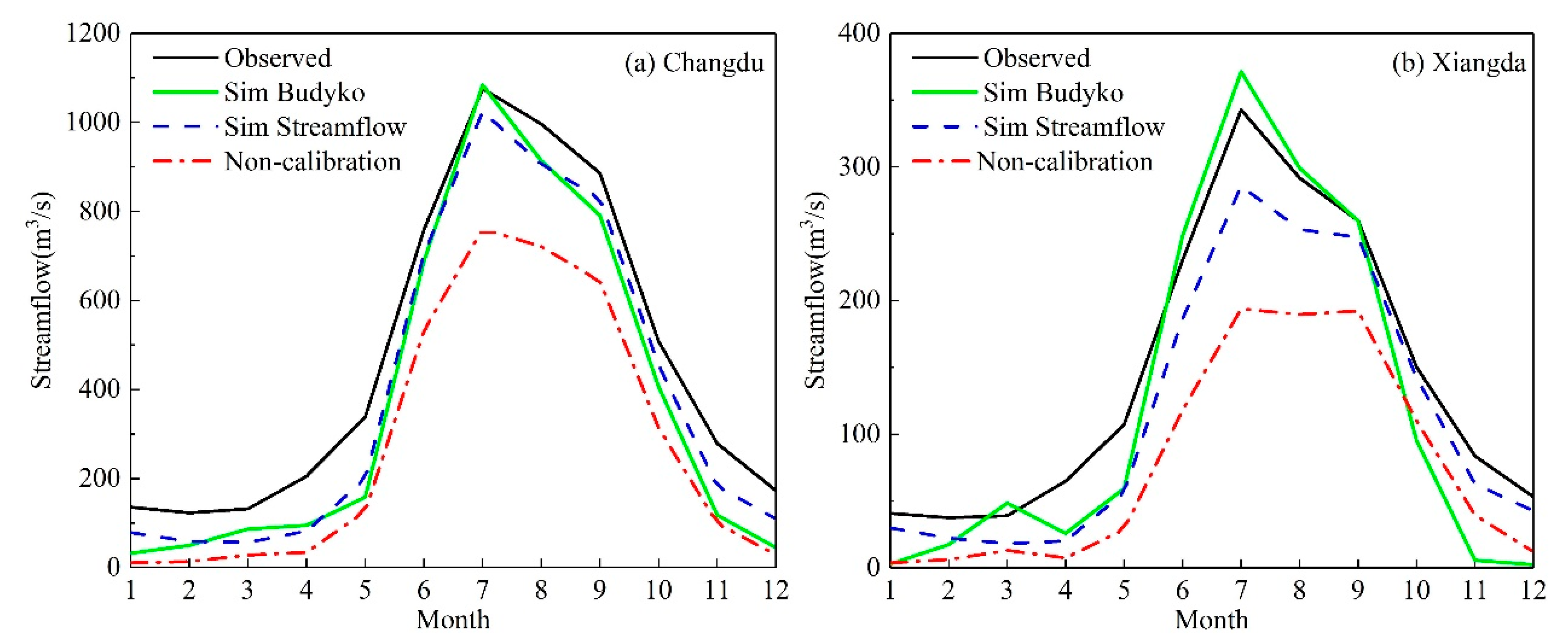
Figure 6 shows the average monthly streamflow hydrograph simulated with different calibration methods. It is observed that the two cases of calibration approaches resulted in good performance of the simulated monthly streamflow in the test catchment. All calibrated approaches provided better results than the non-calibrated model. In the wet season, the simulation results of the monthly average streamflow for the ‘Sim Budyko’ and ‘Sim streamflow’ calibrations are close to the measured data and are far superior to the non-calibration model. However, in the dry season, the simulation results of the model are relatively poor. The reason is that SWAT suffers from the aforementioned disadvantages (i.e., poor model performance in the dry season, large differences between dry and rainy season) [75]. It should be noted that there are two main reasons for the poor performance of the model in the dry season. First, the calibrated objective functions tend to rely on flood characteristics and do not take into account dry periods. Second, the temporal variation of the sub-watershed model parameters is not considered. For example, Muleta found that the sensitivities of the main parameters of the SWAT model were significantly different in dry and wet periods [76]. Additionally, as reported in studies using other hydrological models, model efficiency is consistently lower during dry periods than during wet periods [77].
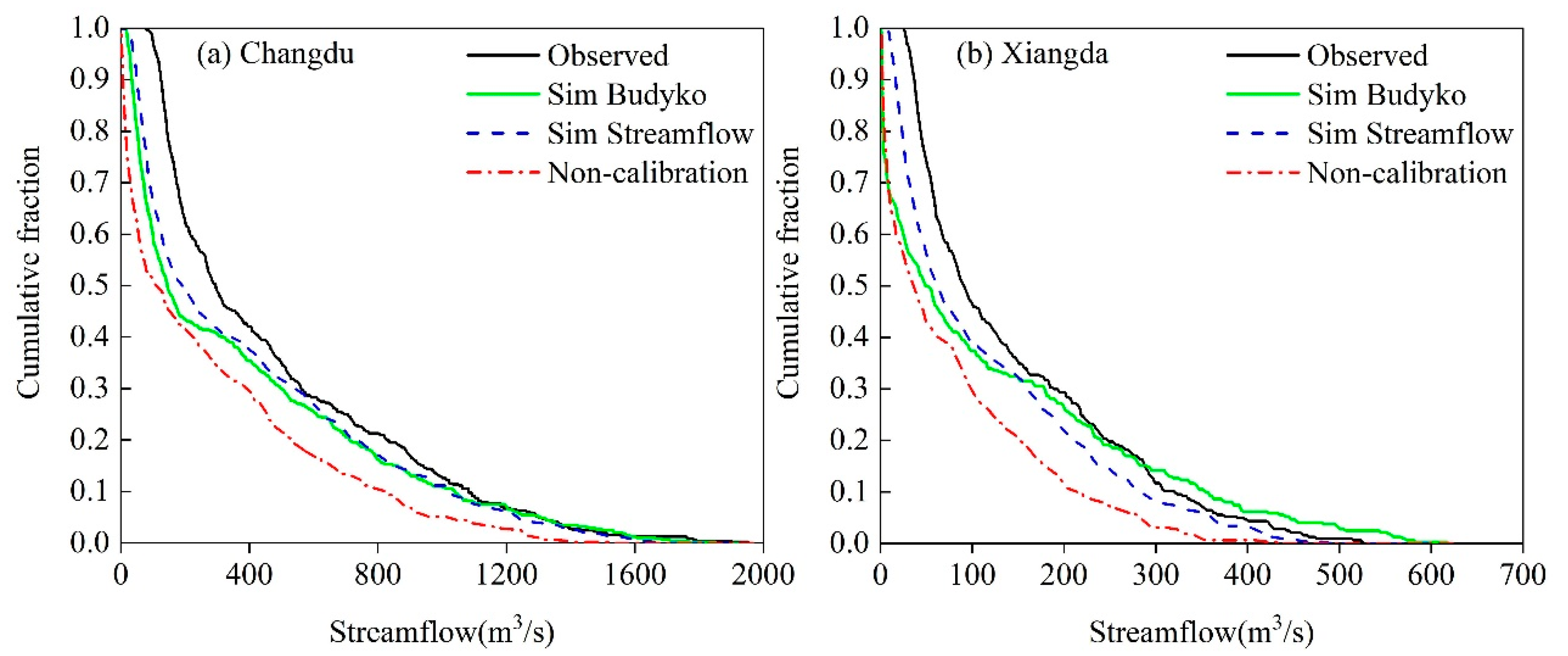
The empirical cumulative density function (CDF) of the monthly runoff distribution for the three calibration methods was calculated. Flow duration curves of simulated and observed values are often used and compared to assess the goodness of fit of the model. Figure 7 shows the CDF of the monthly streamflow of the three calibration approaches. It is apparent that the ‘Sim Budyko’ and ‘Sim streamflow’ calibrations offered a good fit. The simulation result is good in the high streamflow period, but worse in the low streamflow period. However, the portion of the curve related to streamflow shows a large discrepancy between simulated and observed values indicates poor simulation performance during the dry season.
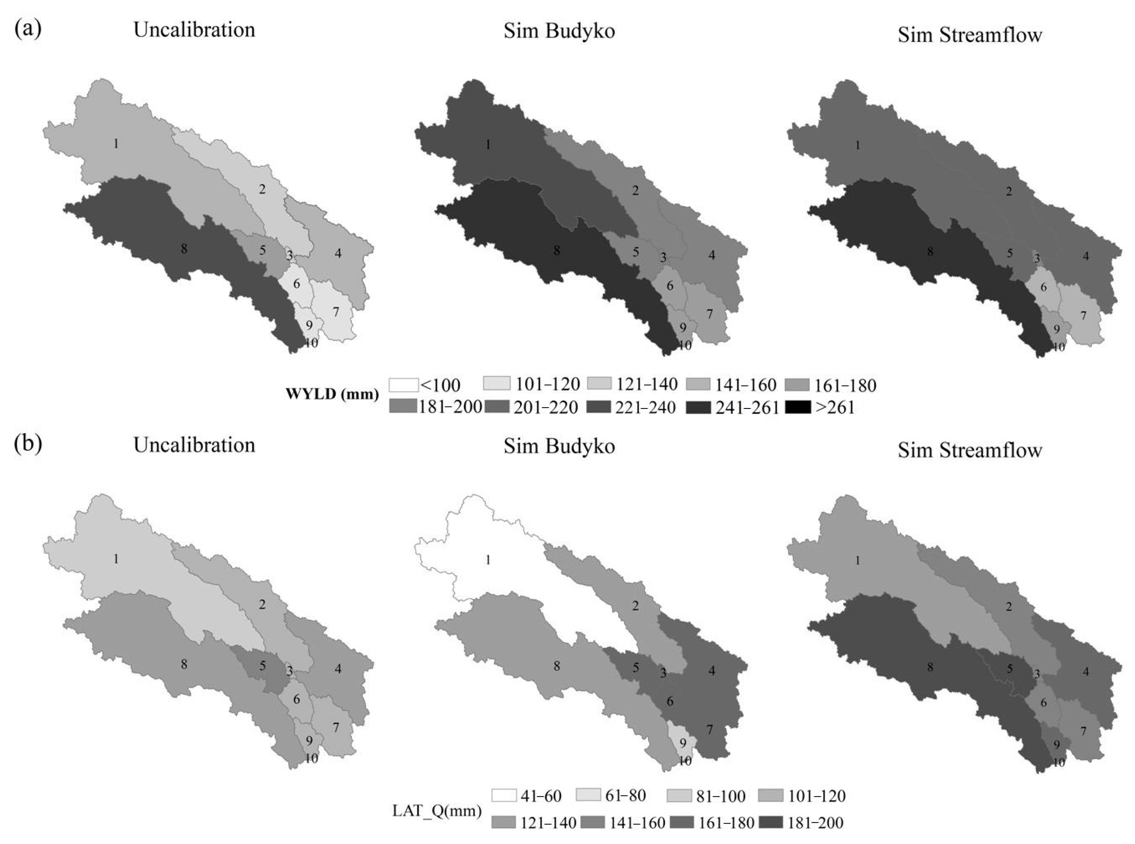
Water yield is one of the important parameters estimated by this model for effective water resource management and when planning the research area. The contribution made by each sub-basin in the watershed area to the total water yield during the simulation period was examined using the three calibration approaches (Sim Budyko, Sim streamflow and non-calibration). Figure 8 shows the water yield and lateral flow spatial variation of sub-basins in the period of 1961~2013. The average annual water yield of the UL-MR obtained by ‘Sim Budyko’ calibration and ‘Sim streamflow’ calibration is close; the results are, respectively, 192.6 and 195.6 mm. However, the average annual water yield of the UL-MR obtained by ‘uncalibration’ is only 135.8 mm. The water yield spatial variation of sub-basins obtained by ‘Sim Budyko’ calibration and ‘Sim streamflow’ calibration is basically consistent. It was noted that sub-basin 8 has the highest water yield of above 240 mm. The lateral flow obtained based on the ‘Sim Budyko’ calibration is obviously different from the ‘Sim streamflow’ calibration, because the ‘Sim Budyko’ calibration fails to fully consider the influence of the concentration parameters. The lateral flow was higher in the high infiltration region and lower in flat land. It was observed that the southwest region contributed a high lateral flow to streamflow.
4.3. Comparison of Calibrated Parameters
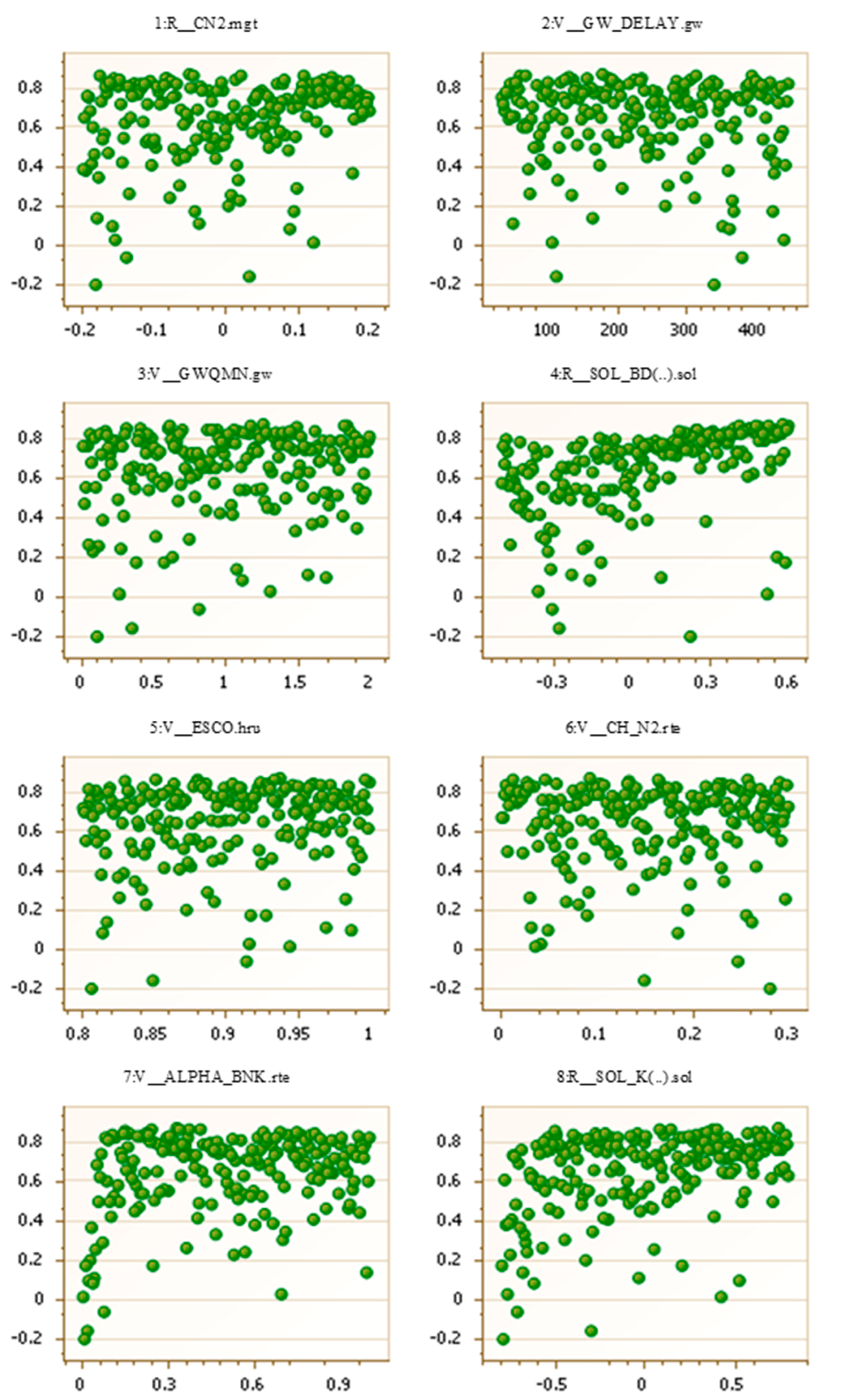
The sensitivity of the parameters was evaluated by considering the p-value [68]. For ‘Sim Budyko’ calibration, three parameters (SOL_K(1), SOL_BD(1), CN2) were significantly sensitive at low p-values (<0.05) during the calibration period for most sub-basins (Table 5). The remaining parameters were found to have no significant impact on discharge simulations and caused no significant changes in the model surface runoff output with p-values > 0.05, thus increasing model uncertainties in the catchment. For ‘Sim streamflow’ calibration, Figure 9 shows the relationship between parameters and objective function using NSE. Each graph shows the NS value as a function of the eight parameter values. Looking at the scatter plots created during calibration, significant distribution parameter values were observed for most of the parameters according to the global sensitivity analysis. In regions with a high NSE, many parameters exhibit equifinality phenomenon. These features also show that most parameters in the model simulation results have low uncertainty. However, model parameters CN2, SOL_K(1) and SOL_BD(1) were more distinguishable, showing more variance than the other parameters. It should be noted that the degree of aggregation of NSE decreases as the values of the CN2, SOL_K(1) and SOL_BD(1) decrease, which indicates that the CN2, SOL_K(1) and SOL_BD(1) have a significant effect on the uncertainty of the simulation results. This indicated that the remaining model parameters were the primary source of streamflow uncertainty in the UL-MR. We should fully understand the real structure information of the model to reduce errors caused by the structure and parameters uncertainty. The SWAT model runs on a large number of parameters to account for uncertainties, and the large number of parameters further complicates the process of the model’s parameterization and calibration [49].
Table 6 shows the optimal values of the calibration parameters of the different calibration approaches using SWAT-CUP. The ‘Sim Budyko’ parameter value is the average of all sub-basins. The models using different calibration methods had different optimal parameter sets; however, upon closer inspection, we found that the values of both parameter sets were very different. In other words, the model using different calibration methods still yielded similarly good performance but had different optimal parameter values. This reflects the effect of parameter equifinality [78]. In general, the calibrated parameters using observed streamflow and water yield were different. For example, the ‘Sim Budyko’ calibration led to a decrease in the value of the CN2 parameter by 4%, respectively, whereas the ‘Sim streamflow’ calibration led to a slight increase in CN2 by 4%. An increase in CN2 generally leads to an increase in runoff in the model. For the GW_DELAY, the two calibration approaches produced similarly large values, which resulted in slower recharge and discharge to rivers from shallow aquifers [79]. The GWQMN represents base flow and its value decreased from 1.94 to 1.15. Regarding channel parameters, the CH_N2 increased from 0.12 to 0.19 and the ALPHA_BNK increased from 0.19 to 0.28; a larger ALPHA_BNK value results in greater bank storage, which contributes to the flow reaching the main channel or sub-basin. The channel water routing parameters (CH_N2, ALPHA_BNK) were not sensitive to the objective function of the Budyko calibration because the Budyko calibration takes more consideration of runoff generation and evaporation at the sub-basin scale; the routing processes and the runoff concentration are not sensitive to the objective function of the Budyko calibration. The ESCO is an important parameter related to soil evaporation, and as the ESCO value decreased from 1.00 to 0.86, the model was able to extract a greater evaporation demand from the lower levels. The parameter SOL_AWC is the effective water capacity of the soil layer, and its value decreased from 0.94 to 0.51. A reduction in SOL_AWC usually results in a reduction in runoff [65].
In summary, during the calibration, the different parameter values compensated for the difference in different calibration approaches, resulting in good consistency with the observed streamflow at the outlet of the basin. This can lead to different hydrological compartments (e.g., surface runoff, base flow, and groundwater flow). Therefore, although the traditional calibration and Budyko calibration provided good fits between the simulated and observed streamflow, the division of the water balance components may differ for different calibration approaches [68]. Numerous studies have already emphasized that modeling other water balance components with models calibrated only with outlet flow should be used with great caution [80]. This is the inherent limitation of calibrating and validating a model based on only flow at the outlet of the watershed. It is important to validate models using other hydrological components such as snow coverage measurements, soil moisture and satellite-based evapotranspiration [81]. If there are sufficient data, a multi-site and multi-objective calibration should be performed to remove this uncertainty [81]. In this regard, research has been carried out to explore whether combining remote sensing datasets with spatially distributed datasets can improve the overall performance of the hydrological model in some regions [82]. Topics in multi-variable and multi-site calibration are of great interest to us and we plan to conduct further studies on this topic in ungauged mountain basins in the Tibetan Plateau.
5. Conclusions
Due to the lack of ground-based measurements in many mountainous areas in the Tibetan Plateau, this study assessed the potential of calibrating the UL-MR hydrological model using the Budyko framework for the UL-MR. Furthermore, the SWAT model was calibrated using the water yield data. The Budyko calibration approach was compared with the traditional calibration and non-calibration approaches and the model performances for simulating streamflow were determined. This approach is independent of the observed streamflow data and provides more realistic water projections in ungauged basins. We reached the following main conclusions: (1) the simple parameterization of the basin-specific ω resulted in better performance in modeling annual evapotranspiration than the original Budyko model (ω=2.6); (2) the Budyko calibration approach, which considered the variation in the parameter ω, achieved satisfactory simulation of daily streamflow and further proved the applicability of the SWAT model in the mountain watershed; (3) using different calibration approaches resulted in different optimal parameters; therefore, simulations of other water balance components in the model calibrated only with outlet flow should be used with great caution. Multi-site and multi-objective calibration is a promising approach for minimizing uncertainties.
We believe that the proposed approach is a valuable tool for predicting the streamflow in watersheds with no data. In addition, the performance of the Budyko calibration approach requires further investigation under different temporal and spatial scales, and the added value of the currently available satellite products in limiting calibration and the spatial assessment of hydrological models should be further explored, particularly in sparsely gauged and ungauged mountain basins.
Author Contributions
Conceptualization, Z.Y.; methodology, Z.Y.; writing—original draft preparation, Z.Y.; writing—review and editing, X.C. and J.W.; supervision, X.C.; funding acquisition, X.C. and J.W. All authors have read and agreed to the published version of the manuscript.
Funding
This research support by the National Natural Science Foundation of China (Grant No. U1911204, 51861125203), National Key R&D Program of China (2021YFC3001000), Natural Science Foundation of Jiangsu Province, China (Grant No. BK20210652).
Institutional Review Board Statement
Not applicable.
Informed Consent Statement
Not applicable.
Data Availability Statement
Not applicable.
Conflicts of Interest
The authors declare no conflict of interest.
References
- Viviroli, D.; Dürr, H.H.; Messerli, B.; Meybeck, M.; Weingartner, R. Mountains of the world, water towers for humanity: Typology, mapping, and global significance. Water Resour. Res. 2007, 43, W07447. [Google Scholar] [CrossRef] [Green Version]
- Yu, Z.; Wu, J.; Chen, X. An approach to revising the climate forecast system reanalysis rainfall data in a sparsely-gauged mountain basin. Atmos. Res. 2019, 220, 194–205. [Google Scholar] [CrossRef]
- Huss, M.; Farinotti, D.; Bauder, A.; Funk, M. Modelling runoff from highly glacierized alpine drainage basins in a changing climate. Hydrol. Process. 2008, 22, 3888–3902. [Google Scholar] [CrossRef]
- Shinohara, Y.; Kumagai, T.; Otsuki, K.; Kume, A.; Wada, N. Impact of climate change on runoff from a mid-latitude mountainous catchment in central Japan. Hydrol. Process. 2009, 23, 1418–1429. [Google Scholar] [CrossRef] [Green Version]
- Satgé, F.; Bonnet, M.; Gosset, M.; Molina, J.; Lima, W.H.Y.; Zolá, R.P. Assessment of satellite rainfall products over the Andean plateau. Atmos. Res. 2016, 167, 1–14. [Google Scholar] [CrossRef]
- Shortridge, J.E.; Guikema, S.D.; Zaitchik, B.F. Machine learning methods for empirical streamflow simulation: A comparison of model accuracy, interpretability, and uncertainty in seasonal watersheds. Hydrol. Earth Syst. Sci. 2016, 20, 2611–2628. [Google Scholar] [CrossRef] [Green Version]
- Xu, Q.; Chen, J.; Peart, M.R.; Ng, C.N.; Hau, B.C.; Law, W.W. Exploration of severities of rainfall and runoff extremes in ungauged catchments: A case study of Lai Chi Wo in Hong Kong, China. Sci. Total Environ. 2018, 634, 640–649. [Google Scholar] [CrossRef]
- Choubin, B.; Solaimani, K.; Rezanezhad, F.; Roshan, M.H.; Malekian, A.; Shamshirband, S. Streamflow regionalization using a similarity approach in ungauged basins: Application of the geo-environmental signatures in the Karkheh River Basin, Iran. Catena 2019, 182, 104128. [Google Scholar] [CrossRef]
- Ragettli, S.; Zhou, J.; Wang, H.; Liu, C.; Guo, L. Modeling flash floods in ungauged mountain catchments of China: A decision tree learning approach for parameter regionalization. J. Hydrol. 2017, 555, 330–346. [Google Scholar] [CrossRef]
- Mohamoud, Y.M. Prediction of daily flow duration curves and streamflow for ungauged catchments using regional flow duration curves. Hydrol. Sci. J. 2008, 53, 706–724. [Google Scholar] [CrossRef]
- Sang, J.; Allen, P.; Dunbar, J.; Arnold, J.G.; White, J.D. Sediment Yield Dynamics during the 1950s Multi-Year Droughts from Two Ungauged Basins in the Edwards Plateau, Texas. J. Water Resour. Prot. 2015, 7, 1345–1362. [Google Scholar] [CrossRef] [Green Version]
- Bergström, S. Principles and Confidence in Hydrological Modelling. Hydrol. Res. 1991, 22, 123–136. [Google Scholar] [CrossRef]
- Blöschl, G.; Sivapalan, M.; Wagener, T.; Viglione, A.; Savenije, H. Runoff Prediction in Ungauged Basins: Synthesis across Processes, Places and Scales; Cambridge University Press: Cambridge, UK, 2013. [Google Scholar]
- Sun, W.; Ishidaira, H.; Bastola, S. Calibration of hydrological models in ungauged basins based on satellite radar altimetry observations of river water level. Hydrol. Process. 2012, 26, 3524–3537. [Google Scholar] [CrossRef]
- Hrachowitz, M.; Savenije, H.H.G.; Blöschl, G.; Mcdonnell, J.J.; Sivapalan, M.; Pomeroy, J.W.; Arheimer, B.; Blume, T.; Clark, M.P.; Ehret, U.; et al. A decade of Predictions in Ungauged Basins (PUB)—A review. Hydrol. Sci. J. 2013, 58, 1198–1255. [Google Scholar] [CrossRef]
- Lebecherel, L.; Andréassian, V.; Perrin, C. On evaluating the robustness of spatial-proximity-based regionalization methods. J. Hydrol. 2016, 539, 196–203. [Google Scholar] [CrossRef] [Green Version]
- Swain, J.B.; Patra, K.C. Streamflow estimation in ungauged catchments using regionalization techniques. J. Hydrol. 2017, 554, 420–433. [Google Scholar] [CrossRef]
- Oudin, L.; Andréassian, V.; Perrin, C.; Michel, C.; Le Moine, N. Spatial proximity, physical similarity, regression and ungaged catchments: A comparison of regionalization approaches based on 913 French catchments. Water Resour. Res. 2008, 44, W03413. [Google Scholar] [CrossRef]
- Athira, P.; Sudheer, K.P.; Cibin, R.; Chaubey, I. Predictions in ungauged basins: An approach for regionalization of hydrological models considering the probability distribution of model parameters. Stoch. Environ. Res. Risk Assess. 2016, 30, 1131–1149. [Google Scholar] [CrossRef]
- Lee, H.; McIntyre, N.; Kim, J.; Kim, S.; Lee, H. Prediction of Typhoon-Induced Flood Flows at Ungauged Catchments Using Simple Regression and Generalized Estimating Equation Approaches. Water 2018, 10, 647. [Google Scholar] [CrossRef] [Green Version]
- Ouali, D.; Cannon, A.J. Correction to: Estimation of rainfall intensity–duration–frequency curves at ungauged locations using quantile regression methods. Stoch. Environ. Res. Risk Assess. 2018, 32, 2837. [Google Scholar] [CrossRef]
- Grimaldi, S.; Li, Y.; Pauwels, V.R.N.; Walker, J.P. Remote Sensing-Derived Water Extent and Level to Constrain Hydraulic Flood Forecasting Models: Opportunities and Challenges. Surv. Geophys. 2016, 37, 977–1034. [Google Scholar] [CrossRef]
- Zhang, Y.; Chiew, F.H.S.; Zhang, L.; Li, H. Use of Remotely Sensed Actual Evapotranspiration to Improve Rainfall-Runoff Modeling in Southeast Australia. J. Hydrometeorol. 2009, 10, 969–980. [Google Scholar] [CrossRef]
- Li, Y.; Grimaldi, S.; Pauwels, V.R.N.; Walker, J.P. Hydrologic model calibration using remotely sensed soil moisture and discharge measurements: The impact on predictions at gauged and ungauged locations. J. Hydrol. 2018, 557, 897–909. [Google Scholar] [CrossRef]
- Bai, P.; Liu, X.; Liu, C. Improving hydrological simulations by incorporating GRACE data for model calibration. J. Hydrol. 2018, 557, 291–304. [Google Scholar] [CrossRef]
- Gleason, C.J.; Smith, L.C.; Lee, J. Retrieval of river discharge solely from satellite imagery and at-many-stations hydraulic geometry: Sensitivity to river form and optimization parameters. Water Resour. Res. 2014, 50, 9604–9619. [Google Scholar] [CrossRef]
- Qiu, L.; You, J.; Qiao, F.; Peng, D. Simulation of snowmelt runoff in ungauged basins based on MODIS: A case study in the Lhasa River basin. Stoch. Environ. Res. Risk Assess. 2014, 28, 1577–1585. [Google Scholar] [CrossRef]
- Li, H.; Zhang, Y.; Chiew, F.H.S.; Xu, S. Predicting runoff in ungauged catchments by using Xinanjiang model with MODIS leaf area index. J. Hydrol. 2009, 370, 155–162. [Google Scholar] [CrossRef]
- Du, J.P.; Sun, R. Estimation of evapotranspiration for ungauged areas using MODIS measurements and GLDAS data. Procedia Environ. Sci. 2012, 13, 1718–1727. [Google Scholar] [CrossRef] [Green Version]
- Donohue, R.J.; Roderick, M.L.; McVicar, T.R. On the importance of including vegetation dynamics in Budyko’s hydrological model. Hydrol. Earth Syst. Sci. 2007, 11, 983–995. [Google Scholar] [CrossRef] [Green Version]
- Lee, S.; Kim, S.U. Quantification of hydrological responses due to climate change and human activities over various time scales in South Korea. Water 2017, 9, 34. [Google Scholar] [CrossRef]
- Mianabadi, A.; Davary., K.; Pourreza-Bilondi., M.; Coenders-Gerrits, A.M.J. Budyko framework; towards non-steady state conditions. J. Hydrol. 2020, 588, 125089. [Google Scholar] [CrossRef]
- Fu, B.P. On the calculation of the evaporation from land surface. Sci. Atmos. Sin. 1981, 5, 23–31. (In Chinese) [Google Scholar]
- Jiang, C.; Xiong, L.; Wang, D.; Liu, P.; Guo, S.; Xu, C.Y. Separating the impacts of climate change and human activities on runoff using the Budyko-type equations with time-varying parameters. J. Hydrol. 2015, 522, 326–338. [Google Scholar] [CrossRef]
- Yang, D.; Shao, W.; Yeh, P.J.F.; Yang, H.; Kanae, S.; Oki, T. Impact of vegetation coverage on regional water balance in the nonhumid regions of China. Water Resour. Res. 2009, 45, 450–455. [Google Scholar] [CrossRef] [Green Version]
- Greve, P.; Burek, P.; Wada, Y. Using the Budyko framework for calibrating a global hydrological model. Water Resour. Res. 2020, 56, e2019WR026280. [Google Scholar] [CrossRef]
- Li, D.; Pan, M.; Cong, Z.; Wood, E. Vegetation control on water and energy balance within the Budyko framework. Water Resour. Res. 2013, 49, 969–976. [Google Scholar] [CrossRef]
- Greve, P.; Gudmundsson, L.; Orlowsky, B.; Seneviratne, S.I. Introducing a probabilistic Budyko framework. Geophys. Res. Lett. 2015, 42, 2261–2269. [Google Scholar] [CrossRef]
- Zhang, S.; Yang, H.; Yang, D.; Jayawardena, A.W. Quantifying the effect of vegetation change on the regional water balance within the Budyko Framework. Geophys. Res. Lett. 2016, 43, 1140–1148. [Google Scholar] [CrossRef]
- Berry, S.L.; Mackey, B. On modelling the relationship between vegetation greenness and water balance and land use change. Sci. Rep. 2018, 8, 9066. [Google Scholar] [CrossRef]
- Sun, F.B. Study on Watershed Evapotranspiration Based on the Budyko Hypothesis. Ph.D. Thesis, Tsinghua University, Beijing, China, 2007. (In Chinese). [Google Scholar]
- Devia, G.K.; Ganasri, B.P.; Dwarakish, G.S. A Review on Hydrological Models. Aquat. Procedia 2015, 4, 1001–1007. [Google Scholar] [CrossRef]
- Kumari, N.; Srivastava, A.; Sahoo, B.; Raghuwanshi, N.S.; Bretreger, D. Identification of suitable hydrological models for streamflow assessment in the Kangsabati River Basin, India, by using different model selection scores. Nat. Resour. Res. 2021, 30, 4187–4205. [Google Scholar] [CrossRef]
- Darbandsari, P.; Coulibaly, P. Inter-comparison of lumped hydrological models in data-scarce watersheds using different precipitation forcing data sets: Case study of Northern Ontario, Canada. J. Hydrol.-Reg. Stud. 2020, 31, 100730. [Google Scholar] [CrossRef]
- Gudowicz, J. Influence of spatial data quality on modelling of water circulation in the Parseta drainage basin. Rocz. Geomatyki XIV 2016, 4, 437–446. [Google Scholar]
- Gassman, P.W.; Reyes, M.R.; Green, C.H.; Arnold, J.G. The Soil and Water Assessment Tool: Historical Development, Applications, and Future Research Directions. Trans. ASABE 2007, 50, 1211–1250. [Google Scholar] [CrossRef] [Green Version]
- Luo, Y.; Ficklin, D.L.; Liu, X.; Zhang, M. Assessment of climate change impacts on hydrology and water quality with a watershed modeling approach. Sci. Total Environ. 2013, 450, 72–82. [Google Scholar] [CrossRef]
- Francesconi, W.; Srinivasan, R.; Pérez-Miñana, E.; Willcock, S.P.; Quintero, M. Using the Soil and Water Assessment Tool (SWAT) to model ecosystem services: A systematic review. J. Hydrol. 2016, 535, 625–636. [Google Scholar] [CrossRef]
- Lin, F.; Chen, X.; Yao, H.; Lin, F. SWAT model-based quantification of the impact of land-use change on forest-regulated water flow. Catena 2022, 211, 105975. [Google Scholar] [CrossRef]
- Li, J.; Bortolot, Z.J. Quantifying the impacts of land cover change on catchment-scale urban flooding by classifying aerial images. J. Clean. Prod. 2022, 344, 130992. [Google Scholar] [CrossRef]
- Abbaspour, K.C.; Rouholahnejad, E.; Vaghefi, S.; Srinivasan, R.; Yang, H.; Kløve, B. A continental-scale hydrology and water quality model for Europe: Calibration and uncertainty of a high-resolution large-scale SWAT model. J. Hydrol. 2015, 524, 733–752. [Google Scholar] [CrossRef] [Green Version]
- Qi, J.; Li, S.; Li, Q.; Xing, Z.; Bourque, C.P.A.; Meng, F.R. Assessing an Enhanced Version of SWAT on Water Quantity and Quality Simulation in Regions with Seasonal Snow Cover. Water Resour. Manag. 2016, 30, 5021–5037. [Google Scholar] [CrossRef]
- Wang, Y.; Bian, J.; Zhao, Y.; Tang, J.; Jia, Z. Assessment of future climate change impacts on nonpoint source pollution in snowmelt period for a cold area using SWAT. Sci. Rep. 2018, 8, 2402. [Google Scholar] [CrossRef] [PubMed] [Green Version]
- Malagò, A.; Bouraoui, F.; De Roo, A. Diagnosis and Treatment of the SWAT Hydrological Response Using the Budyko Framework. Sustainability 2018, 10, 1373. [Google Scholar] [CrossRef]
- He, Z.; Hu, H.; Tian, F.; Ni, G.; Hu, Q. Correcting the TRMM rainfall product for hydrological modelling in sparsely-gauged mountainous basins. Hydrol. Sci. J. 2017, 62, 306–318. [Google Scholar] [CrossRef]
- MRC. State of the Basin Report 2010; Mekong River Commission: Vientiane, Laos, 2010. [Google Scholar]
- Zhou, C.; Guan, Z. The source of lancangjiang (mekong) river. Geogr. Res. 2001, 20, 184–190. (In Chinese) [Google Scholar]
- Buermann, W.; Dong, J.; Zhou, L.; Zeng, X.; Dickinson, R.E.; Potter, C.S.; Myneni, R.B. Analysis of a Multi-year Global Vegetation Leaf Area Index Data Set. J. Geophys. Res. Atmos. 2002, 107, 4646. [Google Scholar] [CrossRef] [Green Version]
- Wang, D.; Alimohammadi, N. Responses of annual runoff, evaporation, and storage change to climate variability at the watershed scale. Water Resour. Res. 2012, 48, 5546. [Google Scholar] [CrossRef] [Green Version]
- Allen, R.G.; Pereira, L.S.; Raes, D.; Smith, M. Crop Evapotranspiration-Guidelines for Computing Crop Water Requirements-FAO Irrigation and Drainage Paper 56; FAO: Rome, Italy, 1998; Volume 300, p. D05109. [Google Scholar]
- Gutman, G.; Ignatov, A. The derivation of the green vegetation fraction from NOAA/AVHRR data for use in numerical weather prediction models. Int. J. Remote Sens. 1998, 19, 1533–1543. [Google Scholar] [CrossRef]
- Zhang, Y.; Zhang, S.; Zhai, X.; Xia, J. Runoff variation and its response to climate change in the Three Rivers Source Region. J. Geogr. Sci. 2012, 22, 781–794. [Google Scholar] [CrossRef]
- Maier, N.; Dietrich, J. Using SWAT for Strategic Planning of Basin Scale Irrigation Control Policies: A Case Study from a Humid Region in Northern Germany. Water Resour. Manag. 2016, 30, 3285–3298. [Google Scholar] [CrossRef]
- Malagó, A.; Bouraoui, F.; Vigiak, O.; Grizzetti, B.; Grizzetti, B.; Pastori, M. Modelling water and nutrient fluxes in the Danube River Basin with SWAT. Sci. Total Environ. 2017, 603, 196–218. [Google Scholar] [CrossRef] [PubMed]
- Neitsch, S.L.; Arnold, J.G.; Kiniry, J.R.; Williams, J.R. Soil and Water Assessment Tool Theoretical Documentation Version 2009; Texas Water Resources Institute Technical Repor No. 406; Texas A&M University: College Station, TX, USA, 2011. [Google Scholar]
- Mockus, V. National Engineering Handbook, Section 4: Hydrology; US Soil Conservation Service: Washington, DC, USA, 1972.
- Penman, H.L.; Keen, B.A. Natural evaporation from open water, bare soil and grass. Proceedings of the Royal Society of London. Series, A. Math. Phys. Sci. 1948, 193, 120–145. [Google Scholar]
- Tuo, Y.; Duan, Z.; Disse, M.; Chiogna, G. Evaluation of precipitation input for SWAT modeling in Alpine catchment: A case study in the Adige river basin (Italy). Sci. Total Environ. 2016, 573, 66–82. [Google Scholar] [CrossRef] [PubMed] [Green Version]
- Moriasi, D.N.; Arnold, J.G.; Van Liew, M.W.; Bingner, R.L.; Harmel, R.D.; Veith, T.L. Model evaluation guidelines for systematic quantification of accuracy in watershed simulations. Trans. ASABE 2007, 50, 885–900. [Google Scholar] [CrossRef]
- Seibert, J.; Vis, M.J.P.; Lewis, E.; Meerveld, H.V. Upper and lower benchmarks in hydrological modelling. Hydrol. Process. 2018, 32, 1120–1125. [Google Scholar] [CrossRef]
- Nash, J.E.; Sutcliffe, J.V. River flow forecasting through conceptual models part I—A discussion of principles. J. Hydrol. 1970, 10, 282–290. [Google Scholar] [CrossRef]
- Etter, P.C. Underwater Acoustic Modeling and Simulation; CRC Press: Boca Raton, FL, USA, 2018. [Google Scholar]
- Marco, N.D.; Avesani., D.; Righetti., M.; Zaramella, M.; Majone, B.; Borga, M. Reducing hydrological modelling uncertainty by using MODIS snow cover data and a topography-based distribution function snowmelt model. J. Hydrol. 2021, 599, 126020. [Google Scholar] [CrossRef]
- Bouslihim, Y.; Rochdi, A.; Paaza, N.E.; Liuzzo, L. Understanding the effects of soil data quality on SWAT model performance and hydrological processes in Tamedroust watershed (Morocco). J. Arf. Earth Sci. 2019, 160, 103616. [Google Scholar] [CrossRef]
- Zhang, D.; Chen, X.; Yao, H.; Lin, B. Improved calibration scheme of SWAT by separating wet and dry seasons. Ecol. Model 2015, 301, 54–61. [Google Scholar] [CrossRef] [Green Version]
- Muleta, M.K. Improving Model Performance Using Season-Based Evaluation. J. Hydrol. Eng. 2012, 17, 191–200. [Google Scholar] [CrossRef]
- Demirel, M.; Booij, M.; Hoekstra, A. The skill of seasonal ensemble low-flow forecasts in the Moselle River for three different hydrological models. Hydrol. Earth Syst. Sci. 2015, 19, 275–291. [Google Scholar] [CrossRef] [Green Version]
- Beven, K.; Binley, A. The future of distributed models: Model calibration and uncertainty prediction. Hydrol. Process. 1992, 6, 279–298. [Google Scholar] [CrossRef]
- Radcliffe, D.E.; Mukundan, R. PRISM vs. CFSR Precipitation Data Effects on Calibration and Validation of SWAT Models. J. Am. Water Resour. Assoc. 2017, 53, 89–100. [Google Scholar] [CrossRef]
- Bitew, M.M.; Gebremichael, M. Evaluation of satellite rainfall products through hydrologic simulation in a fully distributed hydrologic model. Water Resour. Res. 2011, 47, W06256. [Google Scholar] [CrossRef]
- Tuo, Y.; Marcolini, G.; Disse, M.; Chiogna, G. A multi-objective approach to improve SWAT model calibration in alpine catchments. J. Hydrol. 2018, 559, 347–360. [Google Scholar] [CrossRef]
- Herman, M.R.; Nejadhashemi, A.P.; Abouali, M.; Hernandez-Suarez, J.S.; Daneshvar, F.; Zhang, Z. Evaluating the role of evapotranspiration remote sensing data in improving hydrological modeling predictability. J. Hydrol. 2018, 556, 39–49. [Google Scholar] [CrossRef]
Figure 1.
Location of the research basin and spatial distribution of the stations.

Figure 2.
(a) Landuse and (b) soil classes maps used in Soil Water Assessment Tool (SWAT).

Figure 3.
Flowchart of calibrating SWAT model based on Budyko framework.

Figure 4.
Budyko’s curves for the UL-MR. The dots represent the data of the basins in the UL-MR interpolated by Fu’s curves. The Budyko limit curve is dashed. The red dots represent the results of the actual streamflow calibration, the green dots represent the results of the Budyko calibration, and the blue dots represent the results of non-calibrated model.

Figure 5.
Observed and simulated monthly streamflow for different calibration approaches((Sim Budyko, Sim Streamflow, Non-calibration)) in the UL-MR. (a) Changdu hydrological station; (b) Xiangda hydrological station.
Figure 5.
Observed and simulated monthly streamflow for different calibration approaches((Sim Budyko, Sim Streamflow, Non-calibration)) in the UL-MR. (a) Changdu hydrological station; (b) Xiangda hydrological station.

Figure 6.
Average monthly streamflow hydrograph simulated with different calibration approaches (Sim Budyko, Sim streamflow, non-calibration) in the UL-MR. (a) Changdu hydrological station; (b) Xiangda hydrological station.
Figure 6.
Average monthly streamflow hydrograph simulated with different calibration approaches (Sim Budyko, Sim streamflow, non-calibration) in the UL-MR. (a) Changdu hydrological station; (b) Xiangda hydrological station.

Figure 7.
Cumulative distribution functions of monthly streamflow of the three calibration approaches (Sim Budyko, Sim Streamflow, Non-calibration). (a) Changdu hydrological station; (b) Xiangda hydrological station.
Figure 7.
Cumulative distribution functions of monthly streamflow of the three calibration approaches (Sim Budyko, Sim Streamflow, Non-calibration). (a) Changdu hydrological station; (b) Xiangda hydrological station.

Figure 8.
(a)Lateral flow and (b)water yield spatial variation of sub-basins for 1961~2013. Numbers represent subbasins code.
Figure 8.
(a)Lateral flow and (b)water yield spatial variation of sub-basins for 1961~2013. Numbers represent subbasins code.

Figure 9.
Objective function NSE versus sensitive parameters showing the sensitivity of model parameters for streamflow.
Figure 9.
Objective function NSE versus sensitive parameters showing the sensitivity of model parameters for streamflow.


Table 1.
Summary of hydrological and meteorological stations.
| Station Type | Station Name | Latitude | Longitude | Elevation (m) | Data Length |
|---|---|---|---|---|---|
| Hydrological stations | Xiangda | 32°15′ | 96°28′ | 4050 | 1961–1981; 2008–2013 |
| Changdu | 31°11′ | 97°11′ | 3306 | 1961–1981; 1983–1988; 1991–2007 | |
| Meteorological stations | Zaduo | 32°54′ | 95°18′ | 4066 | 1961–2013 |
| Yushu | 33°25′ | 97°03′ | 3681 | ||
| Suoxian | 31°53′ | 93°47′ | 4022 | ||
| Dingqing | 31°25′ | 95°36′ | 3873 | ||
| Nangqian | 32°12′ | 96°29′ | 3643 | ||
| Changdu | 31°11′ | 97°11′ | 3306 |
Table 2.
Data sources and description.
| Data type | Scale | Data Source |
|---|---|---|
| DEM | 90 m × 90 m | Shuttle Radar Topography Mission (SRTM) produced by Consortium for Spatial Information (CGIAR-CSI) |
| Land use map | 30 m × 30 m | Chinese Academy of Science |
| Soil map | 1:1500,000 | Food and Agriculture Organization (FAO) |
| Climate input | Meteorological Data Center of the China Meteorological Administration | |
| Monthly streamflow | Meteorology Agency and Water Conservation Agency of Qinghai Province | |
| NDVI | 1000 m × 1000 m | National Oceanic &Atmospheric Administration (NOAA) (http://www.noaa.gov, (accessed on 1 May 2021)) |
Table 3.
Parameters for calibrating the SWAT models with different calibration approaches.
| Category | Parameter Name | Definition |
|---|---|---|
| Runoff | CN2.mgt | SCS runoff curve number |
| Groundwater | GW_DELAY.gw | Groundwater delays (days) |
| GWQMN.gw | Threshold depth of water in the shallow aquifer required for return flow to occur (mm) | |
| Soil | ESCO.hru | Soil evaporation compensation factor |
| SOL_BD(1) | Moist bulk density (g/cm3) | |
| SOL_K(1) | Soil conductivity (mm/h) | |
| Channel | CH_N2.rte | Manning’s “n” value for the main channel |
| ALPHA_BNK.rte | Baseflow alpha factor for bank storage(days) |
Table 4.
Performance of the SWAT model for monthly streamflow simulation using three calibration approaches (Sim Budyko, Sim Streamflow, Non-calibration).
Table 4.
Performance of the SWAT model for monthly streamflow simulation using three calibration approaches (Sim Budyko, Sim Streamflow, Non-calibration).
| Calibration Approaches | Changdu Station | Xiangda Station | ||||||||||
|---|---|---|---|---|---|---|---|---|---|---|---|---|
| Calibration Period (1961–1987) | Validation Period (1988–2007) | Calibration Period (1961–1981) | Validation Period (2008–2013) | |||||||||
| NSE | PBIAS (%) | R2 | NSE | PBIAS (%) | R2 | NSE | PBIAS (%) | R2 | NSE | PBIAS (%) | R2 | |
| Non-calibration | 0.33 | 41.86 | 0.91 | 0.46 | 39.70 | 0.87 | 0.52 | 45.84 | 0.81 | 0.31 | 47.87 | 0.56 |
| Sim Budyko | 0.84 | 22.38 | 0.91 | 0.83 | 17.60 | 0.89 | 0.68 | 15.78 | 0.82 | 0.44 | 14.87 | 0.76 |
| Sim Streamflow | 0.88 | 17.69 | 0.93 | 0.86 | 14.78 | 0.90 | 0.82 | 19.32 | 0.87 | 0.73 | 20.85 | 0.83 |
Table 5.
Sensitivity analysis of SWAT model parameters in different subbasins for the calibration period.
Table 5.
Sensitivity analysis of SWAT model parameters in different subbasins for the calibration period.
| Parameters Name | p-Value | |||||||||
|---|---|---|---|---|---|---|---|---|---|---|
| Sub1 | Sub2 | Sub3 | Sub4 | Sub5 | Sub6 | Sub7 | Sub8 | Sub9 | Sub10 | |
| r_CN2.mgt | 0.00 | 0.02 | 0.00 | 0.00 | 0.33 | 0.59 | 0.01 | 0.50 | 0.00 | 0.01 |
| v_GW_DELAY.gw | 0.07 | 0.12 | 0.13 | 0.49 | 0.20 | 0.17 | 0.18 | 0.18 | 0.09 | 0.28 |
| v_GWQMN.gw | 0.15 | 0.05 | 0.41 | 0.14 | 0.07 | 0.60 | 0.46 | 0.04 | 0.37 | 0.93 |
| v_CH_N2.rte | 0.02 | 0.02 | 0.23 | 0.23 | 0.04 | 0.59 | 0.49 | 0.02 | 0.38 | 0.86 |
| v_ALPHA_BNK.rte | 0.89 | 0.82 | 0.39 | 0.38 | 0.47 | 1.00 | 0.82 | 0.48 | 0.81 | 0.37 |
| v_ESCO.hru | 0.95 | 0.59 | 0.07 | 0.99 | 0.67 | 0.73 | 0.71 | 0.49 | 0.99 | 0.25 |
| r_SOL_K(1).sol | 0.00 | 0.00 | 0.00 | 0.30 | 0.10 | 0.00 | 0.00 | 0.19 | 0.00 | 0.00 |
| r_SOL_BD(1).sol | 0.00 | 0.00 | 0.00 | 0.84 | 0.66 | 0.00 | 0.00 | 0.36 | 0.00 | 0.00 |
Note. The initial letter of the parameter name represents the adjustment method of parameters. “R” denotes the relative change by multiplying and “V” denotes replacement of the initial value.
Table 6.
Optimal parameters calibrated for two calibration approaches.
| Parameters Name | Sim Budyko | Sim Streamflow |
|---|---|---|
| r_CN2.mgt | −0.04 | 0.04 |
| v_GW_DELAY.gw | 303.46 | 442.20 |
| v_GWQMN.gw | 1.15 | 1.94 |
| v_CH_N2.rte | 0.19 | 0.12 |
| v_ALPHA_BNK.rte | 0.28 | 0.19 |
| v_ESCO.hru | 0.86 | 1.00 |
| r_SOL_K(1).sol | 0.51 | 0.94 |
| r_SOL_BD(1).sol | 0.55 | 0.85 |
Note. The initial letter of the parameter name represents the adjustment method of parameters. “R” donates relative change by multiplying and “V” donates replacement of the initial value.
Publisher’s Note: MDPI stays neutral with regard to jurisdictional claims in published maps and institutional affiliations. |
© 2022 by the authors. Licensee MDPI, Basel, Switzerland. This article is an open access article distributed under the terms and conditions of the Creative Commons Attribution (CC BY) license (https://creativecommons.org/licenses/by/4.0/).
Share and Cite
MDPI and ACS Style
Yu, Z.; Chen, X.; Wu, J. Calibrating a Hydrological Model in an Ungauged Mountain Basin with the Budyko Framework. Water 2022, 14, 3112. https://doi.org/10.3390/w14193112
AMA Style
Yu Z, Chen X, Wu J. Calibrating a Hydrological Model in an Ungauged Mountain Basin with the Budyko Framework. Water. 2022; 14(19):3112. https://doi.org/10.3390/w14193112
Chicago/Turabian StyleYu, Zexing, Xiaohong Chen, and Jiefeng Wu. 2022. "Calibrating a Hydrological Model in an Ungauged Mountain Basin with the Budyko Framework" Water 14, no. 19: 3112. https://doi.org/10.3390/w14193112
Note that from the first issue of 2016, this journal uses article numbers instead of page numbers. See further details here.