
Water Hammer in Steel–Plastic Pipes Connected in Series

1
Faculty of Building Services, Hydro and Environmental Engineering, Warsaw University of Technology, 00-653 Warsaw, Poland
2
Faculty of Mechanical Engineering and Mechatronics, West Pomeranian University of Technology in Szczecin, 70-310 Szczecin, Poland
*
Author to whom correspondence should be addressed.
Water 2022, 14(19), 3107; https://doi.org/10.3390/w14193107
Submission received: 31 August 2022
/
Revised: 22 September 2022
/
Accepted: 27 September 2022
/
Published: 2 October 2022
(This article belongs to the Special Issue About an Important Phenomenon—Water Hammer)
Abstract
:This paper experimentally and numerically investigates the water hammer phenomenon in serially connected steel and HDPE pipes with different diameters. The aim of the laboratory tests was to obtain the time history of the pressure head at the downstream end of the pipeline system. Transient tests were conducted on seven different pipeline system configurations. The experimental results show that despite the significantly smaller diameter of the HDPE pipe compared to the steel pipe, introducing an HDPE section makes it possible to suppress the valve-induced pressure surge. By referring to the results of the experimental tests conducted, the comparative numerical calculations were performed using the fixed-grid method of characteristics. To reproduce pressure wave attenuation in a steel pipe, Brunone-Vitkovský instant acceleration-based model of unsteady friction was used. To include the viscoelastic behavior of the HDPE pipe wall, the one-element Kelvin–Voigt model was applied. By calibrating the unsteady friction coefficient and creep parameters, satisfactory agreement between the calculated and observed data was obtained. The calibrated values of parameters for a single experimental test were introduced in a numerical model to simulate the remaining water hammer runs. It was demonstrated that using the same unsteady friction coefficient and creep parameters in slightly different configurations of pipe lengths can be effective. However, this approach fails to reliably reproduce the pressure oscillations in pipeline systems with sections of significantly different lengths.
1. Introduction
Any rapid alteration in the fluid flow velocity results in a pressure wave that propagates through the pipeline system. Such events, known as hydraulic transients or water hammer, can cause serious problems. It is well known that violent pressure surges may lead to pipe bursts, hydraulic device failures or water contamination [1,2]. Due to the fact that pipeline systems are subjected to a wide variety of operating conditions, transient flows commonly occur. For this reason, in recent decades, numerous studies have been conducted on this topic. In practice, pressurized fluid distribution systems often consist of serially connected pipes with different properties, i.e., different pipe-wall materials and different diameters. Nevertheless, to date, only a few researchers have addressed the problem of hydraulic transients in complex multi-pipe systems.
Gong et al. [3] investigated the possibility of replacing a metallic pipe with a plastic section in order to attenuate the pressure waves. They demonstrated that it is feasible to mitigate pressure surges in water distribution systems if the branch that links the transient source and the water main is connected to a plastic section instead of steel pipe. Garg and Kumar [4] studied the water hammer in a pipeline with two different materials and their combined configuration and reported that pipes made of viscoelastic material can be used to renovate existing water pipelines to effectively control the water hammer. Triki [5] proposed a protection technique based on replacing a short section of the transient sensitive regions of the existing piping system by another one made of polymeric material. Ferrante [6] investigated the effect of the junction between two pipes with different polymeric materials on the transient pressure wave and proved that the reflection coefficient at the junction between the two pipes depends on the viscoelastic parameters and on the transient time-history. Bettaieb et al. [7] studied the performance of metallic–polymeric pipe configurations under transient conditions caused by pump failure and demonstrated that wave reflections from junction connections significantly affect the pressure wave in water distribution systems.
Despite this interest, no one—to the best of our knowledge—has studied the water hammer phenomenon in a serially connected steel–plastic pipeline system with significantly different inner diameters and for several different lengths of each section. The present work aimed to experimentally and numerically investigate a valve-induced water hammer phenomenon in serially connected pipes with different properties, in terms of both the pipe dimensions and the pipe-wall material. The measurements were taken on a setup from which it was possible to collect transient data in a pipeline that consisted of steel and high-density polyethylene (HDPE) sections connected in series. Moreover, the experiments were carried out for various lengths of steel and HDPE sections, while maintaining a constant total length of the pipeline system. By referring to the results of the conducted experimental tests, the comparative numerical calculations were performed using the fixed-grid method of characteristics.
This paper is divided into six sections. In the second section, some theoretical aspects of hydraulic transients in pressurized pipes are presented. Experimental tests are outlined in the third section. Numerical calculations are addressed in Section 4 and Section 5. Conclusions are drawn in the final section.
2. Mathematical Description of Hydraulic Transients in Pressure Pipes
The 1D unsteady pressure pipe flow is governed by the system of first-order hyperbolic partial differential equations resulting from mass and momentum conservation [8]:
where f is the friction factor (−), c is the pressure wave velocity (m/s), H is the piezometric head (m), V is the mean flow velocity (m/s), g is the gravity acceleration (m/s2), x is the space coordinate (m), t is time (s), and D is the internal pipe diameter (m).
Equation (1) is the momentum equation and Equation (2) is called the continuity equation. In classic (elastic) water hammer theory, the pressure wave velocity is defined by:
where α is the parameter dependent on the pipe diameter and constraints (−), K is the bulk modulus of elasticity of the liquid (Pa), ρ is the fluid density (m3/s), E is the modulus of elasticity of the pipe-wall material (Pa) and s is the pipe-wall thickness (m).
Traditionally, transient analyses were carried out by incorporating a steady or quasi-steady friction factor into the momentum equation. It is well known that this approach overestimates pressure oscillations during fast transient events [9]. For this reason, the efforts of many researchers have been focused on identifying the dynamic effects accounting for pressure wave damping. Generally, two types of models have been proposed in the literature to reduce discrepancies between the measurements and calculation results: unsteady friction models and viscoelastic models. In the following subsections, the models used in this paper were briefly described.
2.1. Unsteady Friction
In general, two approaches are widely used to take into account unsteady friction: the weighting function-based (WFB) method and instantaneous acceleration-based (IAB) method. The WFB method involves including the friction term in the form of convolution related to the instantaneous flow velocity and to the weighted past velocity changes. This approach, first proposed by Zielke [10] for unsteady laminar flow, was later adapted for transient turbulent flow [11,12]. In the IAB method, the unsteady friction coefficient depends on the local and instantaneous convective acceleration of flowing liquid. Due to its simplicity, probably the best-known example of this method is the model proposed by Brunone [13,14] and later improved by Vítkovský [15] by including an additional sign operator in the convection term. To date, Brunone-Vítkovský model is the only unsteady friction model used in some of the available commercial software tools for simulation of hydraulic transients [16]. In this approach, the friction factor is given by the following equation:
where fq is the quasi-steady friction factor (−), kV is the unsteady friction coefficient (−) and sign(V) = (+ 1 for V > 0 or −1 for V < 0).
The sign term in Equation (4) gives the correct sign of the convective term for all possible flow [17]. The presented approach combines local inertia and wall friction unsteadiness. In order to analytically determine kV, the Vardy and Brown shear decay coefficient can be used [18]:
where for laminar flow, C* is equal to:
and for turbulent flow, C* is given by:
where Re—Reynolds number (−).
2.2. Viscoelastic Behavior of Polymer Pipes
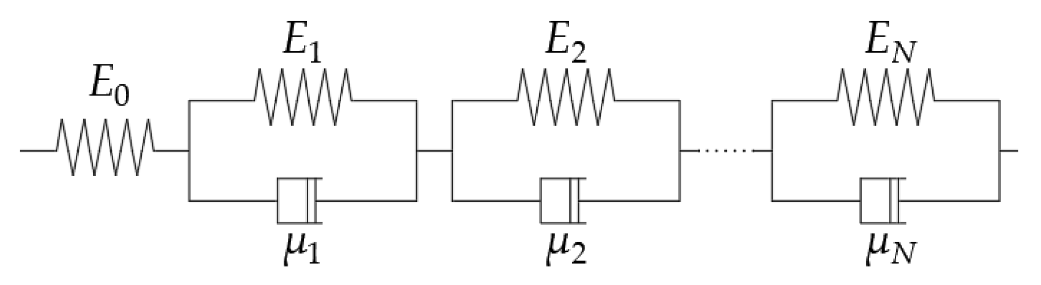
In contrast to elastic materials, viscoelastic materials exhibit a retarded strain after initial instantaneous strain upon applied loading [20]. For this reason, the classic formulation of the continuity equation is no longer suitable for describing unsteady flow in polymer pipes. Polymers exhibit both elastic and viscous characteristics. In order to correctly mathematically describe this property, the response of viscoelastic material is often represented by the mechanical response of an elastic spring connected to the viscous dashpot [21]. This approach, known as “mechanical analogs”, is widely used in simulating hydraulic transients in plastic pipes. Figure 1 presents the scheme of the generalized Kelvin–Voigt model.
Figure 1 shows a series of N Kelvin–Voigt elements with a modulus of elasticity Ek (subscript k denotes the number of a particular element), viscosity of μk, creep compliance Jk = 1/Ek and compliance J0 = 1/E0. The creep function corresponding to the generalized Kelvin–Voigt model is given by:
where τ is the retardation time of the k-th Kelvin–Voigt element (s).
The viscoelasticity of plastic pipes can be incorporated by adding a retarded strain term to the continuity equation [22,23]:
where ε—radial strain of the k-th Kelvin–Voigt element (−).
Equation (9) and Equation (1) describe the unsteady fluid flow in polymer pipes. Further detailed mathematical description of the 1D viscoelastic behavior of polymer pipes during transient flow can be found, e.g., in [23,24,25]. The analysis of transients in viscoelastic pipelines by means of 2D Kelvin-Voigt model is detailed in [26,27].
3. Laboratory Tests
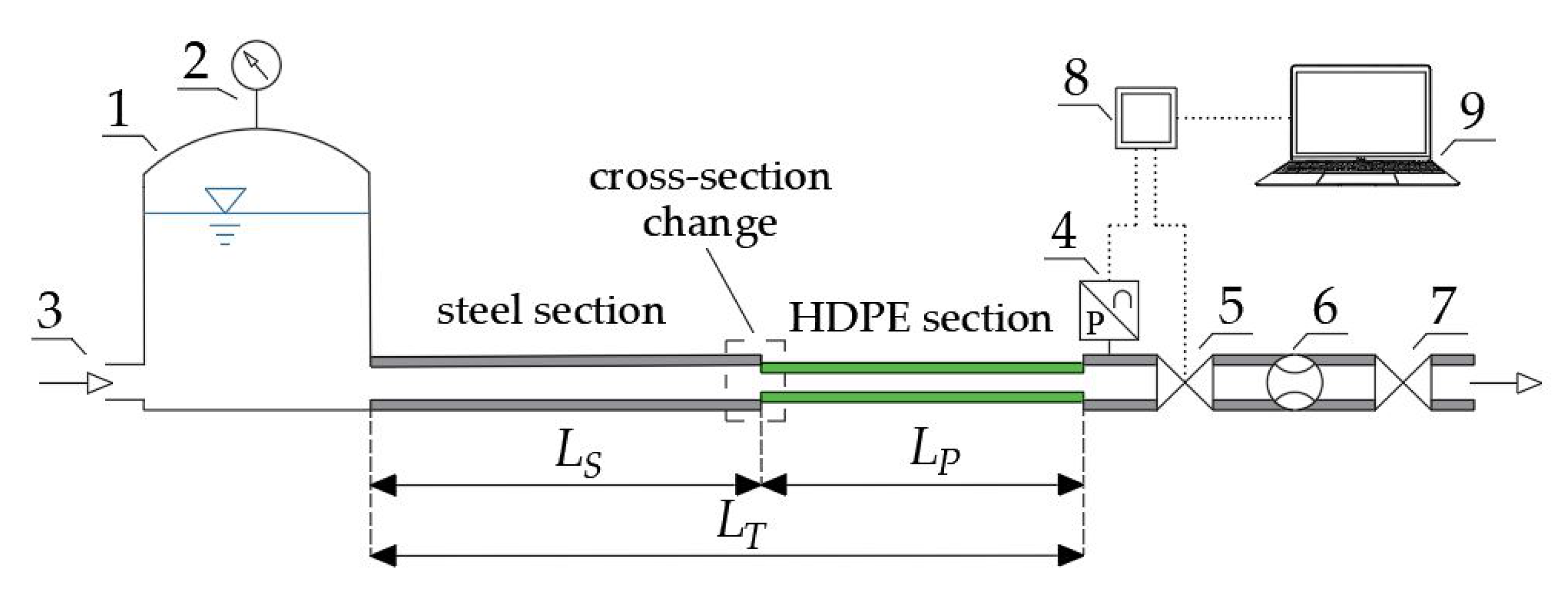
The aim of the experiments presented in this paper was to record pressure changes during a valve-induced water hammer in a horizontal pipeline system that consists of serially connected pipes with different pipe-wall materials, with different inner diameters and with different lengths. Transient data were collected on a laboratory setup that consisted of three essential elements: a pressure tank, pipeline with fittings, and data acquisition system. Two different conduits were used—steel pipe with an inner diameter of DS = 0.053 m and HDPE pipe with an inner diameter of DP = 0.032 m and wall thickness of sP = 0.0024 m (DS/DP = 1.65). In order to capture the influence of the length of each section on pressure changes, tests were performed for different proportions of the length of both pipes, keeping the total length of the system constant. To reduce complexity, the order in which the pipes were fitted was always the same, i.e., the steel pipeline was always connected to the pressure tank that supplied the system. The scheme of the laboratory setup is presented in Figure 2.
The valve that initiated the water hammer as well as the pressure sensor were connected to the short steel section at the downstream end of the pipeline system with the same diameter as the main steel pipe. The distances between the end of the HDPE pipe and pressure sensor (element 4 in Figure 2) and between the end of the HDPE and the valve (element 5 in Figure 2) were 10 cm and 30 cm, respectively. All pipeline sections were rigidly fixed to the floor. The data acquisition system consisted of an inductive flowmeter, a piezoresistive pressure sensor with the range of −0.1–1.2 MPa, and a valve closing timer connected to the laptop through a data logger. Pressure samples were recorded with a frequency of 500 Hz. As mentioned before, the main goal was to perform water hammer tests for different lengths of steel and HDPE sections. Six different steel–plastic configurations were considered. An additional water hammer run was conducted in a straight steel pipeline (without any HDPE section). Overall, seven different configurations of the pipeline systems were considered. In order to be able to compare individual experiments, for each pipeline system configuration, the water hammer phenomenon was initiated for a constant steady-state discharge of approximately 9.167 × 10⁻⁴ m3/s. Due to the fact that the water temperature significantly affects the pressure wave during transient flow in plastic pipes [28], the experiments were conducted, taking care to maintain a constant water temperature (19 °C) for each system configuration. The water hammer was initiated by a manual valve closure. For each run, the registered valve closing time was between 0.04–0.11 s. The main parameters of the pipeline system along with the values of the mean flow velocity during steady flow conditions are listed in Table 1.
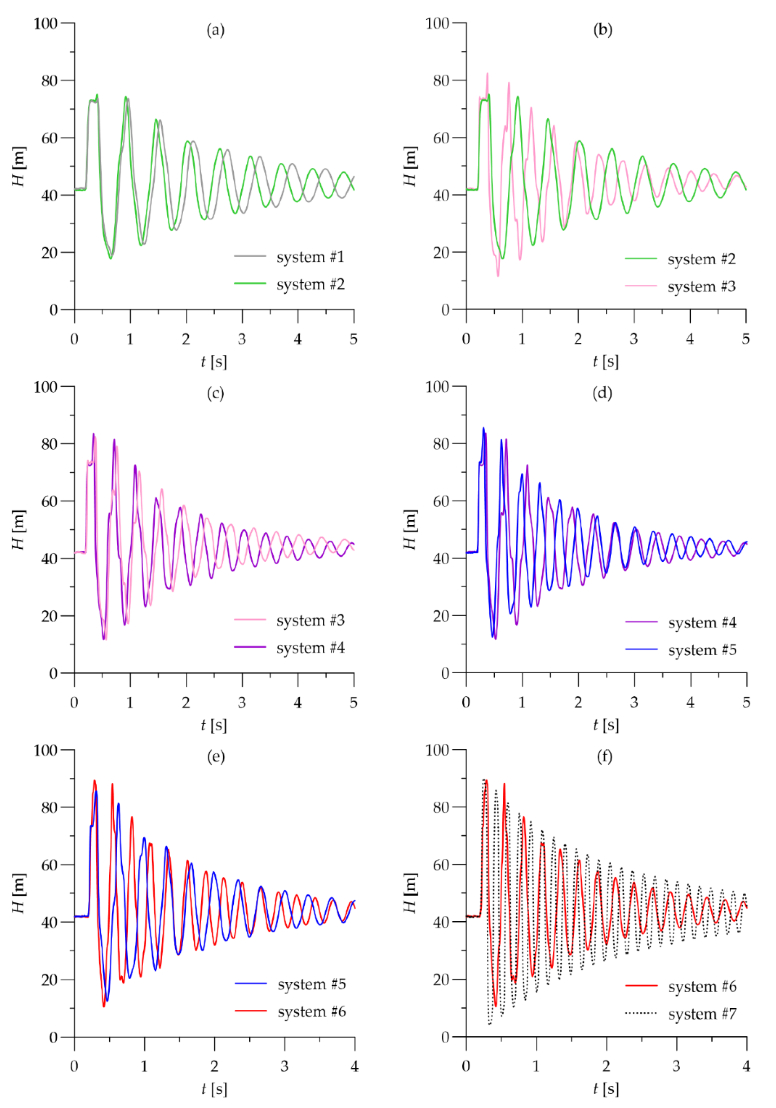
It is worth highlighting that the internal diameters of the pipes used in this setup differ significantly. Hence, for a given initial discharge, the mean flow velocity in the plastic section is much higher than that in the steel section. Since the plastic section is located at the downstream side of the pipeline system and connected near the valve that initiates unsteady flow, this consequently translates into a higher pressure increase during a water hammer event. In order to compare the pressure signals obtained in each water hammer run, the collected transient data are summarized in Figure 3.
As expected, it is apparent from Figure 3 that, with the increase in the share of the steel section in the total length of the pipeline system, the mean pressure wave velocity of the entire pipeline system increases. This can be observed as each subsequent pressure signal shifts to the left, i.e., the return time of the wave reflected from the tank shortens. Interestingly, even despite the much higher initial flow velocity in the HDPE section than in the steel section (during steady state conditions V0P/V0S = 2.26), the maximum pressure increase in each system configuration with a plastic section (systems from #1 to #6) is lower than that in the steel pipeline (system #7). This is due to the viscoelastic properties of the HDPE pipe, which result in less severe transients for the same flow change compared to steel pipe. It can be observed in Figure 3e,f that the second positive pressure peak recorded in system #6 (red line) is practically the same as the first one. Apparently, for this particular LS/LT ratio, the overlapping of pressure waves due to sudden pipeline contraction occurs. Furthermore, similarly to the results of water hammer experiments in viscoelastic pipeline systems with sudden cross-section changes [29,30], the effect of the diameter change is only visible in the first phases of pressure oscillations. Unlike in the case of water hammer in a steel pipeline with sudden contractions and expansions [31], after a couple of consecutive amplitudes, the pressure wave becomes smoothed and resembles oscillations in a simple, single-diameter pipeline. In order to compare differences in the first pressure peak, transient data obtained from all runs are compiled in Figure 4.
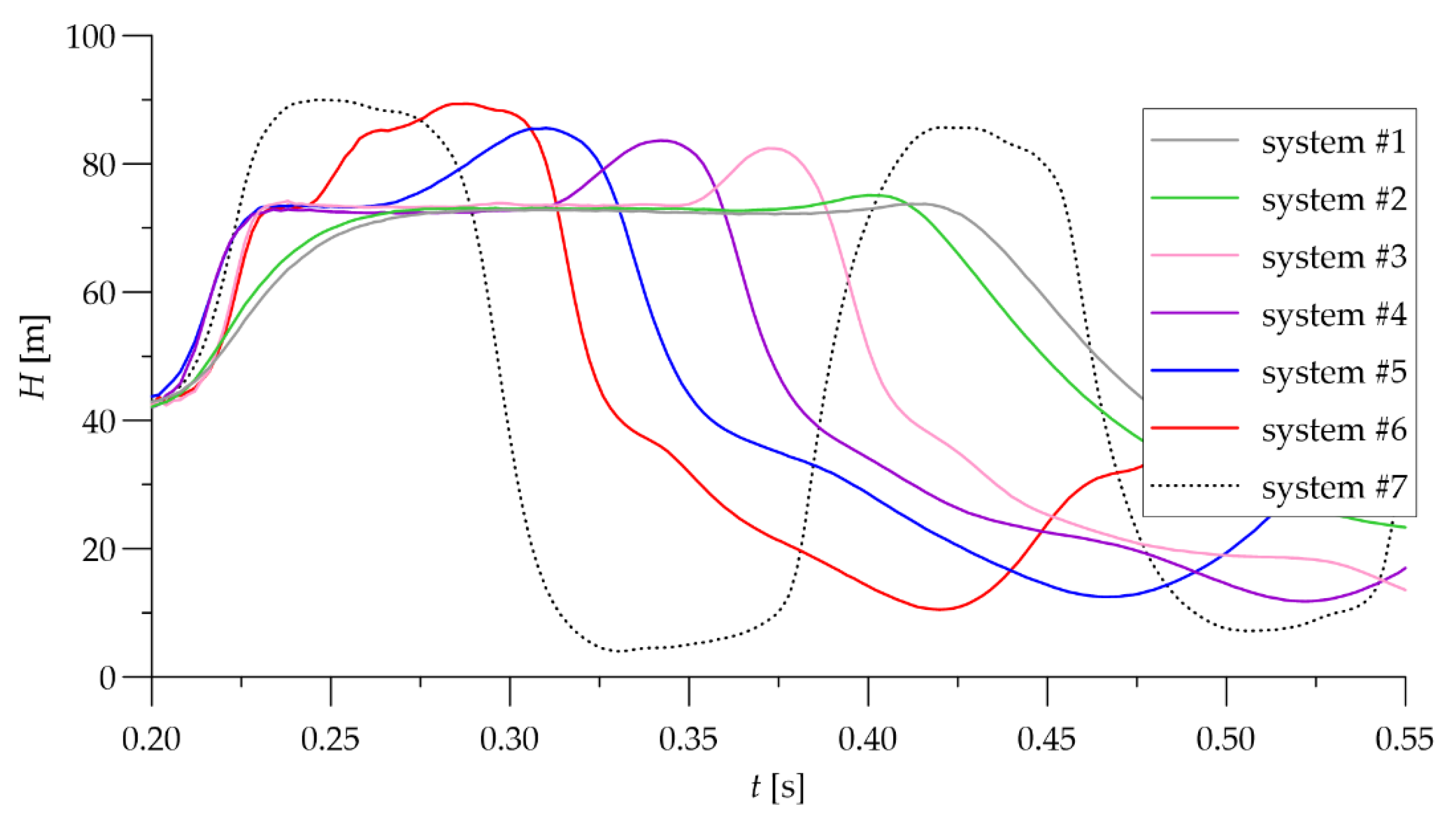
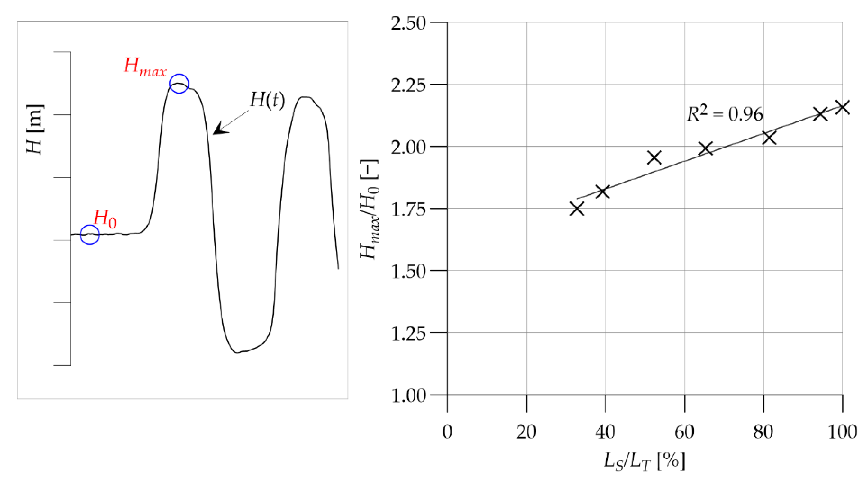
In Figure 4, it can be observed that, in the case of water hammer in systems #1 and #2 (gray and green lines), the H(t) curve becomes almost horizontal for the first half period of the reflection wave. This is typical for viscoelastic pipeline systems and indicates that the pipe-wall material creeps greatly at this time interval [32]. In each case, the interference of pressure waves resulting from the cross-section change is visible. After the first pressure peak, an increase in the pressure level can be observed, which results from the transmission of the pressure wave from a steel section (large diameter) through an HDPE section (small diameter). This effect becomes more significant as the length of the steel section increases, which also affects the maximum pressure rise more. In the pipeline system #1, which has the longest HDPE section, the observed maximum pressure increase is ΔHmax = 31.62 m, whereas in the steel pipeline (system #7), ΔHmax = 48.28 m (where ΔHmax = Hmax − H0). Changes in the dimensionless maximum pressure increase (Hmax/H0) as a function of the LS/LT ratio are presented in Figure 5.
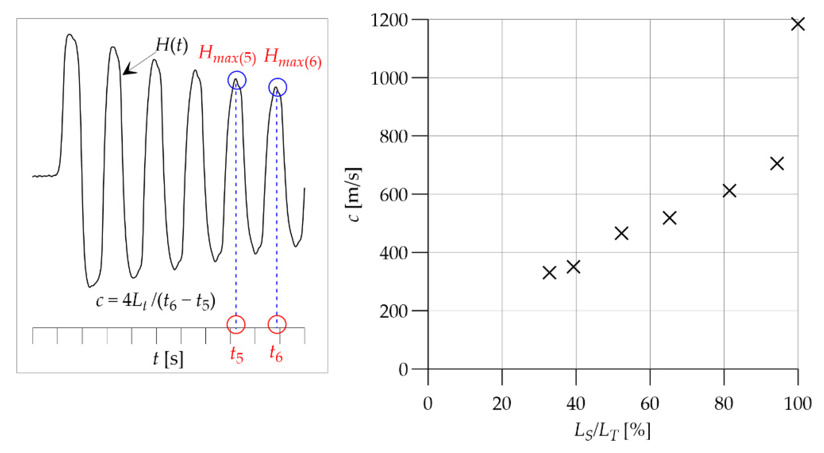
Figure 5 shows a clear trend in the increase in the maximum pressure caused by the lengthening of the steel section. This result indicates that using an in-line polymeric pipe section in order to suppress pressure surges is also possible for pipes with significantly smaller internal diameter compared to the diameter of the original pipe. Evidently, the larger the diameter and longer the length of the polymeric section, the better the pressure wave damping that can be obtained. However, in some fluid distribution systems, increasing the mean flow velocity may be advantageous (e.g., hydraulic transportation systems). In order to analyze the influence of the length of each section on the pressure wave velocity, an attempt to calculate its value was made. The pressure signal obtained from steel–HDPE pipelines is distorted due to sudden cross-section changes. Pressure wave reflections are especially visible in the initial phases of water hammer phenomenon. To minimize the error in the calculation of c, the time difference between the occurrence of the fifth and sixth pressure peaks was taken into account. The results of the calculations are presented as a function of the LS/LT ratio in Figure 6.
As can be seen in Figure 6, for all steel–HDPE pipeline configurations, the pressure wave velocity increases linearly with the increase in the LS/LT ratio. However, for a pipeline system without any HDPE section (system #7; LS/LT = 100%), there is a clear sudden increase in the value of pressure wave velocity. This effect is attributed to the method of determining the value of c presented on the right side of the plot. In principle, the experimentally obtained H(t) signal is a harmonic function with a period equal to the pipeline period of reflection time. In order to calculate the pressure wave velocity, the time interval between successive maximum pressure peaks was taken into account. In fact, this is a measure of the phase speed, not a direct measure of the speed of sound. Despite the limitations of this method of calculating c, Figure 6 to some extent illustrates the changes of pressure wave velocity due to the change in lengths of each section. Detailed discussion on the pressure wave velocity in pipeline systems can be found in [33].
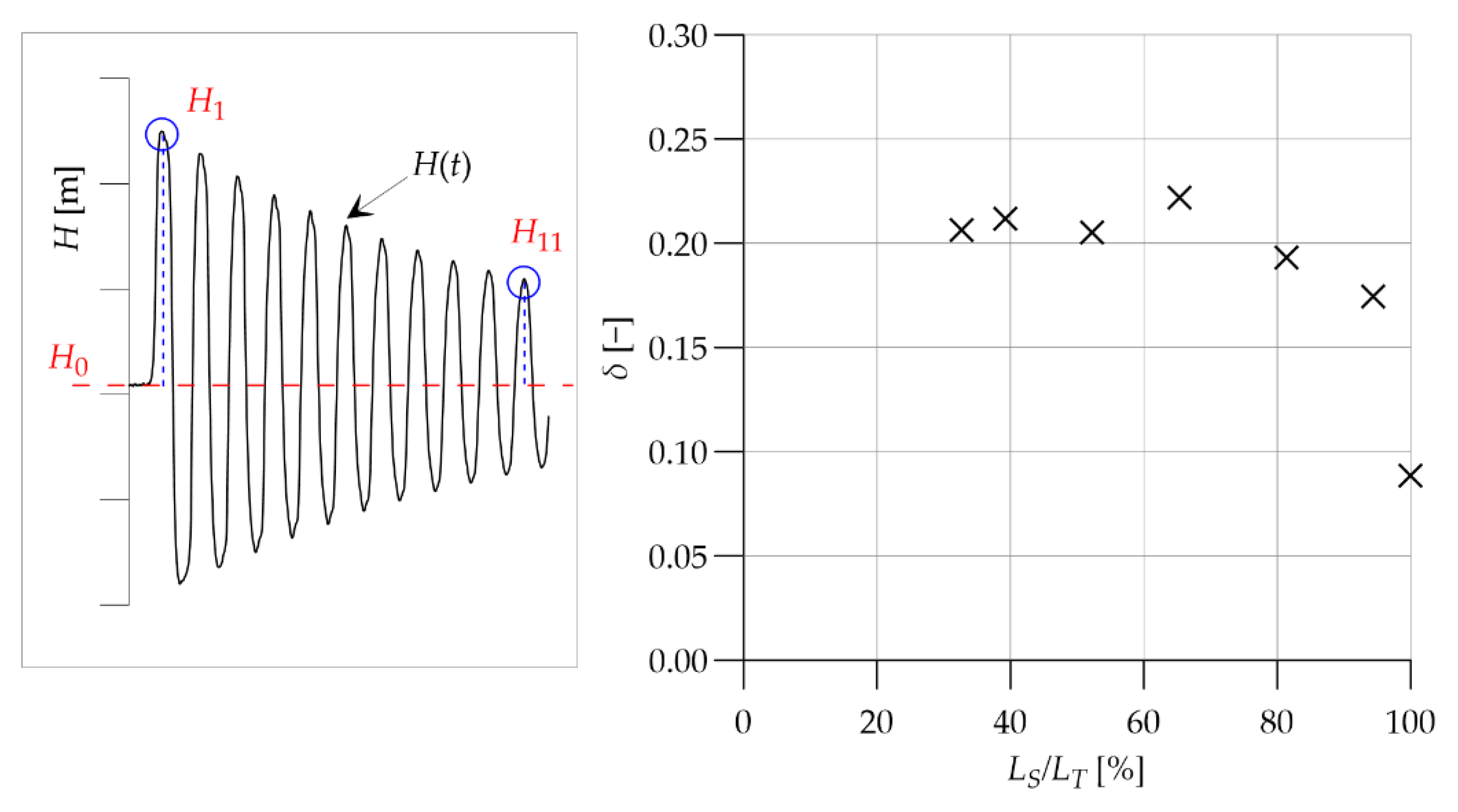
Further analysis of Figure 3 shows that, despite the differences in the values of ΔHmax and c in each water hammer run, the observed pressure wave decays at a similar rate for each steel–HDPE configuration. In order to quantify the damping rate of each particular pipeline system, the logarithmic damping decrement can be calculated as [34]:
where n is the number of subsequent pressure peaks used to calculate the damping decrement and m is the number of the first pressure peak taken into account.
Calculated values of the logarithmic damping decrement for m = 1 and n = 10 are presented in Figure 7.
Figure 7 shows that the pressure magnitudes damped at similar rates for each steel–HDPE pipeline system configuration as the calculated values of δ are between 0.174 and 0.221. As anticipated, the weakest damping of the pressure wave was obtained for the pipeline without any HDPE section (δ = 0.087). It should be noted that no clear correlation between the length of each section and the logarithmic damping decrement was revealed. This is probably due to the cross-section changes, which cause the initial pressure amplitudes not to be damped regularly.
4. Water Hammer Solver
To numerically model the water hammer events obtained during the laboratory tests, a hydraulic transient solver that is able to take into account both the pipe-wall viscoelasticity and unsteady friction presented in [35,36] was used. Here, for brevity, only its simplified description is given.
In most practical cases, the convective acceleration terms and are negligibly small [37]. Hence, simplified governing equations are usually used to numerically simulate hydraulic transients:
where Q is the volumetric flow rate (m3/s).
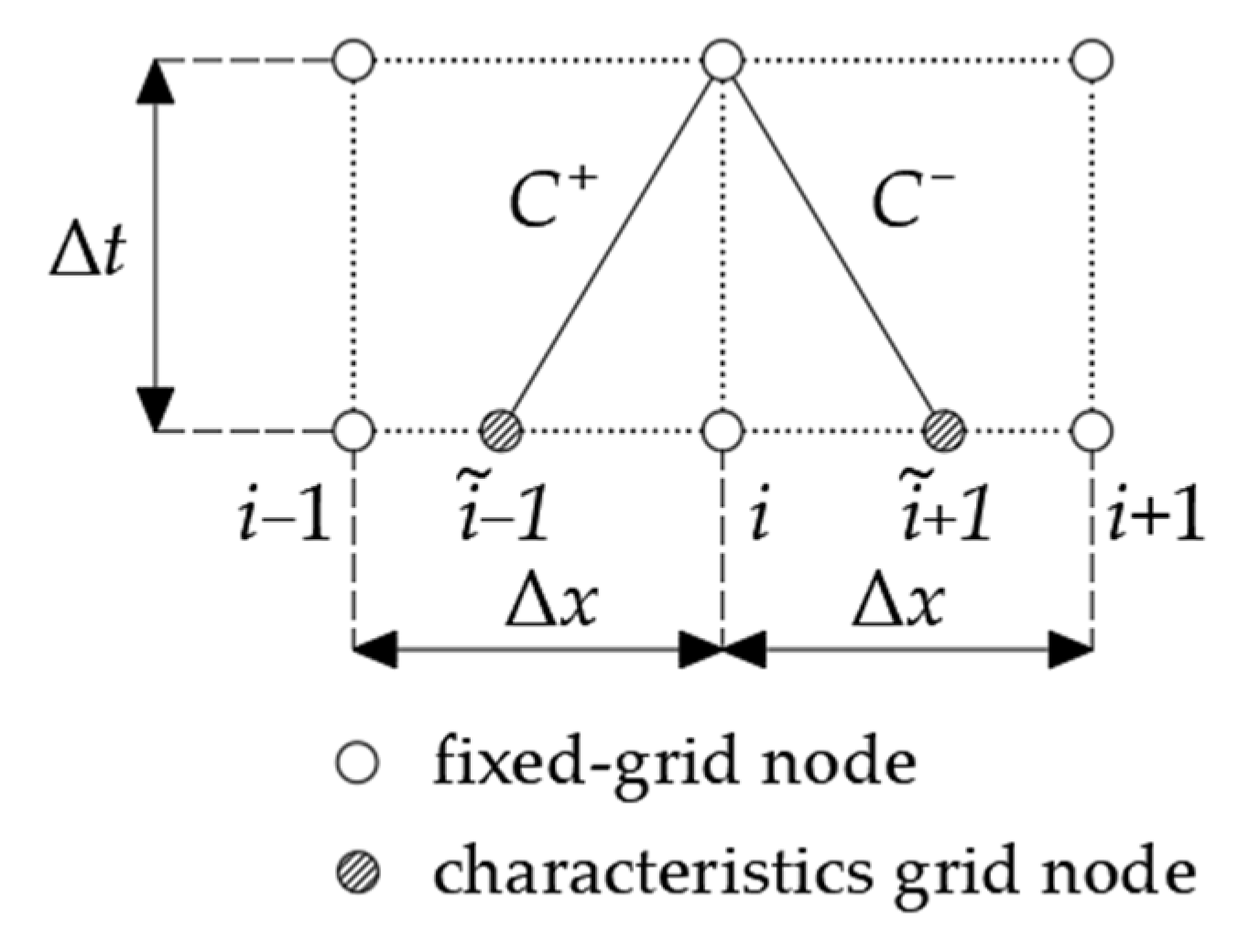
This set of differential equations was solved using the fixed-grid method of characteristics with a specified time interval. A fragment of the uniformly spaced computational grid is presented in Figure 8.
The unknown values of pressure and discharge are calculated from positive and negative characteristics equations:
where CN, Ca+, CP, and Ca− are known coefficients used to describe the steady-state friction, the unsteady friction, and viscoelasticity of the pipe-wall material, respectively.
In general form, these coefficients are defined as:
where parameter B, defined as , depends on the fluid and pipe properties.
In Equations (15)–(17), indexes ′, ″ and ‴ refer to steady-state friction, unsteady friction, and viscoelasticity, respectively. In order to model the pipeline systems used in the experiments, for each section (steel and HDPE), individual computational grids connected with series junction were created. For both sections, steady-state friction was taken into account. For first-order accuracy calculations, the values of and are equal to:
Apart from the steady-state friction term, in each section, different dynamic effects were taken into account. In the steel pipe, Brunone-Vitkovský IAB unsteady friction model described in Section 2.1 was applied. For the HDPE section, unsteady friction was neglected and only the viscoelastic behavior of the pipe-wall material was taken into account. Descriptions of the remaining CN, Ca+, CP, and Ca− coefficients for each section of the pipeline are listed in Table 2.
where γ—volumetric weight of the fluid (kg/m3); θ—relaxation coefficient dependent on a numerical scheme (in our calculations, θ = 1).
Boundary conditions were applied according to [2]. In the first node, a constant level upstream reservoir was assumed. As mentioned before, the connection node between two pipeline sections was defined as a series junction. In the last node, the downstream valve boundary was used, with the relative valve closing function defined as:
where tc—valve closing time (s).
5. Numerical Calculations
The aim of the numerical calculations was to simulate the water hammer runs that were conducted during the experimental study. In all cases, the experimental values of the flow rate, initial pressure, and valve closing time were used as input. The observed pressure signals were used to calibrate the numerical model, i.e., to determine the values of the unsteady friction coefficient and creep parameters that reproduce the observed pressure oscillations. Calibrated values of the parameters for a single experimental test were later introduced in a numerical model to simulate the remaining runs.
The procedure of the numerical calculations was as follows: in the first step, the experiment concerning the water hammer in a steel pipeline without an HDPE section was analyzed (system #7). At this stage, the unsteady friction coefficient kV was calibrated. In the second step of numerical analysis, the pipeline system configuration with the longest HDPE section was considered (system #1). In order to simulate the dynamic effect of pressure wave attenuation in the steel section, the earlier calibrated value of kV was used as an input. The calibration of the model at this stage consisted of determining the creep parameters of the HDPE section which provided good compliance between the observed and calculated H(t) curve. In the third step, the simulations of the remaining experimental configurations were made (systems #2–#6) by using the kV coefficient determined in the first step and the creep parameters calibrated in the second step of the numerical calculations.
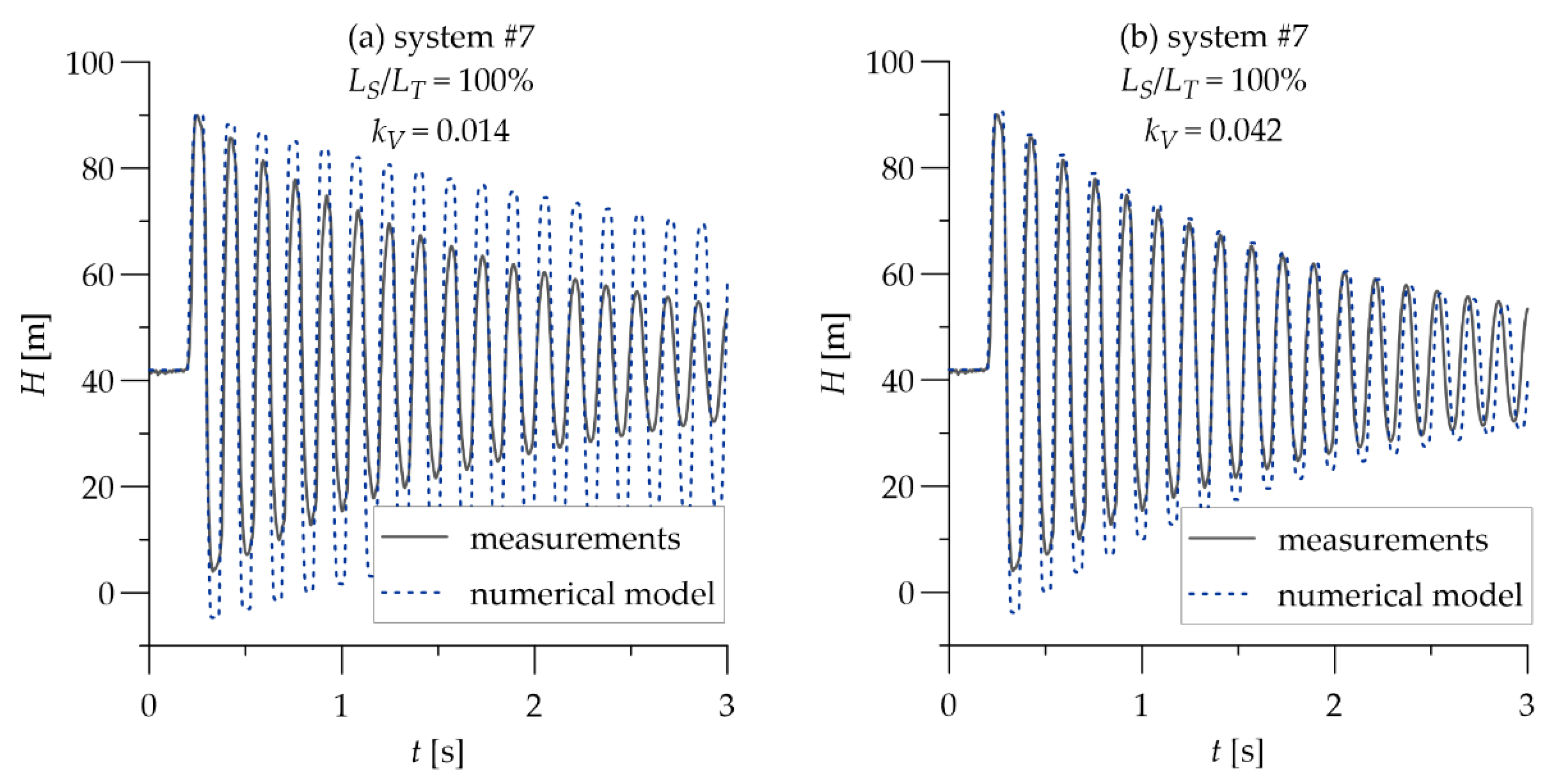
While calibrating the numerical model simulating system #7 (steel pipeline without HDPE section), the lowest discrepancy between the experimental data and the results of numerical calculations was obtained for the pressure wave velocity cS = 1195 m/s and unsteady friction coefficient kV = 0.042. To obtain a stable solution, the CFL condition had to be satisfied. Calculations were made for the space interval in the steel section of ΔxS = 1 m. In order to obtain the Courant number as close as possible to unity, the time interval Δt = 0.00083 s was applied (Ca = 0.99). For comparison, calculations were also performed for kv determined using analytically derived shear decay coefficients (Equations (5) and (7)). The results are presented in Figure 9.
As can be seen in Figure 9a, the calculated pressure oscillations using kv determined with the use of the shear decay coefficient over-predict successive amplitudes of the pressure wave compared to the experimental data. The calibrated value of kv is exactly three times higher than predicted with theoretical formulas. From Figure 9b, it is apparent that for kv = 0.042, satisfactory agreement between the experimental and simulated H(t) curves is obtained.
Turning now to simulating the transient response in the steel–HDPE configuration with the longest plastic section (system #1), the calibration of creep parameters was performed assuming the total number of Kelvin–Voigt elements equal to one. Although in [23] it was indicated that the results obtained for N = 1 are poor, in other works, it was reported that it is possible to obtain satisfactory agreement between the simulated and observed pressure signal with the one-element model [38,39]. As the calibration was performed with a simple “trial and error” method to minimize the square error between the calculated and observed transient data, such simplification considerably facilitates the whole process. The best compliance between the calculations results and measurements in system #1 was obtained for J = 2.20 × 10⁻¹⁰ Pa and τ = 0.034 s. The value of the pressure wave velocity in the HDPE section (also determined by “trial and error” method) used as an input was equal to cP = 300 m/s. To avoid numerical diffusion and dispersion, the space interval applied for the HDPE section was ΔxP = 0.25 m (Ca = 0.99). In numerical calculations simulating hydraulic transients in all steel–plastic configurations, the same value of space interval in the steel section of ΔxS = 1 m and the time interval Δt = 0.00083 s was applied.
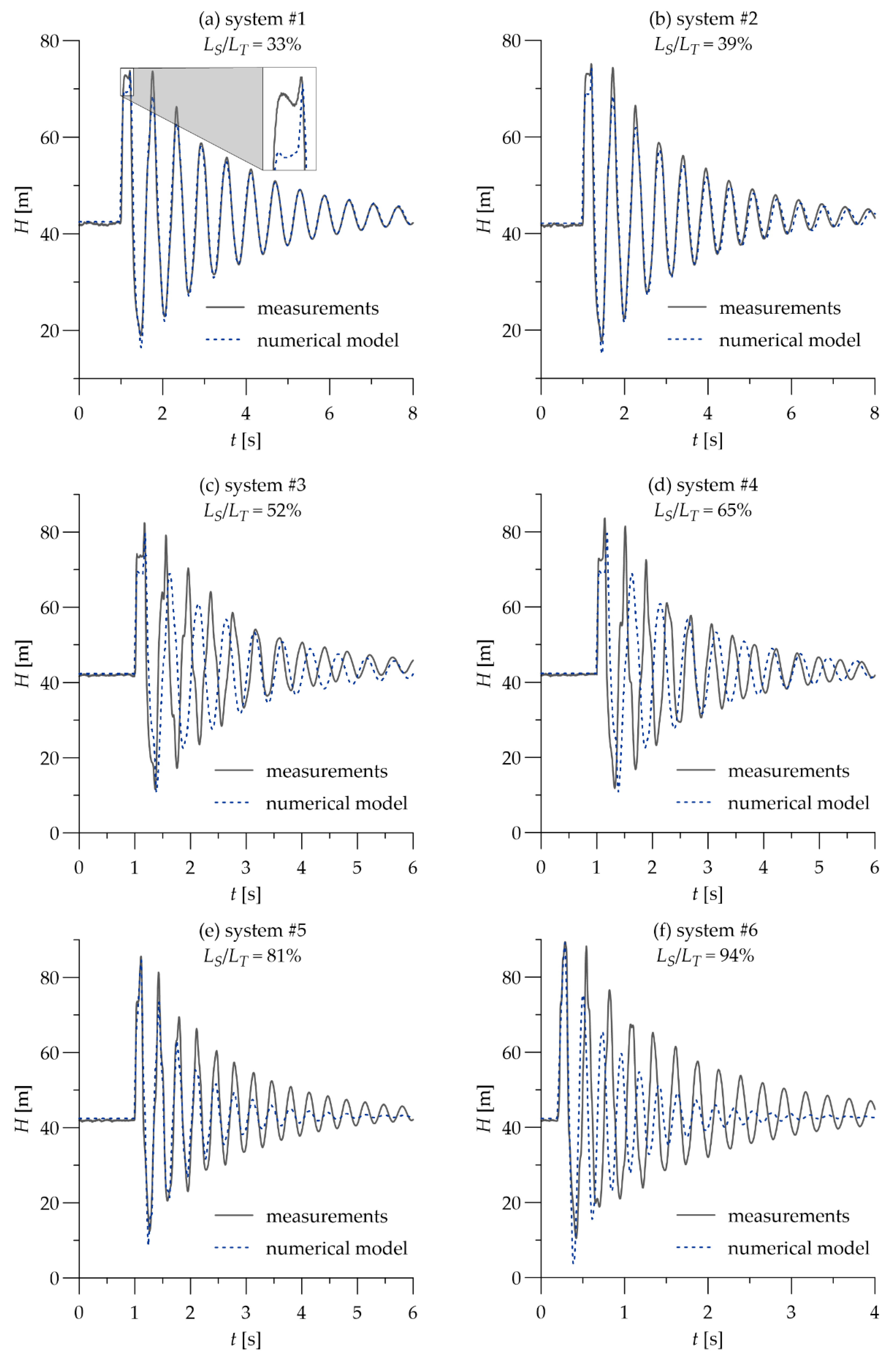
In order to check the suitability of the previously calibrated parameters for pipeline systems with different lengths of each section, calculations simulating tests in the remaining configurations (systems #2–#6) were conducted. A comparison between the calculated and measured pressure oscillations for all steel–HDPE configurations is presented in Figure 10.
The results in Figure 10a show that the approach adopted to simulate a valve-induced water hammer event in the steel–HDPE pipeline can lead to satisfactory results in terms of the simulated pressure oscillations compared to the measured data. It is worth noting that although the phase shift and extreme pressure peaks are reasonably well reproduced, the shape of the calculated first peak differs from the observed one (zoom in Figure 10). This is probably due to the short steel section at the downstream end of the laboratory setup in which the pressure sensor was connected, which was not taken into account in the numerical model. Despite the fact that the distance from the end of the plastic pipe to the pressure sensor was not long, the cross-section change at this section could distort the observed pressure signal. Figure 10b shows that using the same unsteady friction coefficient and creep parameters in a slightly different configuration of pipe section lengths can be effective. The calculated pressure oscillations are similar to the experimental transient data in terms of both the extreme pressures and the effective pressure wave velocity of the entire pipeline system. However, systems #1 and #2 differ only slightly, as the proportion of the length of the steel section to the total pipeline length (LS/LT) is equal to 33% and 39%, respectively.
Figure 10c–f demonstrate that introducing parameters calibrated on a particular pipeline system to a numerical model with significantly different lengths of each section fails to predict the experimental data. Although the maximum and minimum pressure peaks are well reproduced, the shape of the pressure signal differs distinctly. In Figure 10c,d, the calculated effective pressure wave velocity is lower than the observed one as the simulated signal shifts to the right. Interestingly, as can be seen in Figure 10e for LS/LT = 81%, the calculated and experimental H(t) curves have the same pressure wave period time. In the pipeline system with the longest steel section (Figure 10f), the calculated effective pressure wave velocity is higher than the observed one.
Figure 10 shows that, as the share of the steel section in the total length of the pipeline increases, the difference in the damping rate of the calculated and experimental pressure oscillations becomes clearer, i.e., the calculated pressure wave decays faster than the observed one. This is probably related to the fact that the viscoelastic pipe wall’s behavior is more significant in a low-frequency pipeline system [40]. The calibrated values of the creep parameters referred to the pipeline system with the longest HDPE section, in which the pressure wave propagated at a relatively low speed. In such a pipeline system, the plastic pipe has more time to dissipate the energy due to the viscous resistance of HDPE. As observed in the experimental study, the elongation of the steel section causes the pressure wave velocity to increase, and thus, the creep process of the plastic material is disturbed by the returning (reflected from the tank) pressure wave sooner. As a consequence, there is less time for the HDPE section to absorb the energy of the water. This result also supports previous findings presented by Mitosek and Chorzelski [41] who experimentally demonstrated that the pressure wave velocity in viscoelastic pipes strongly depends on their length.
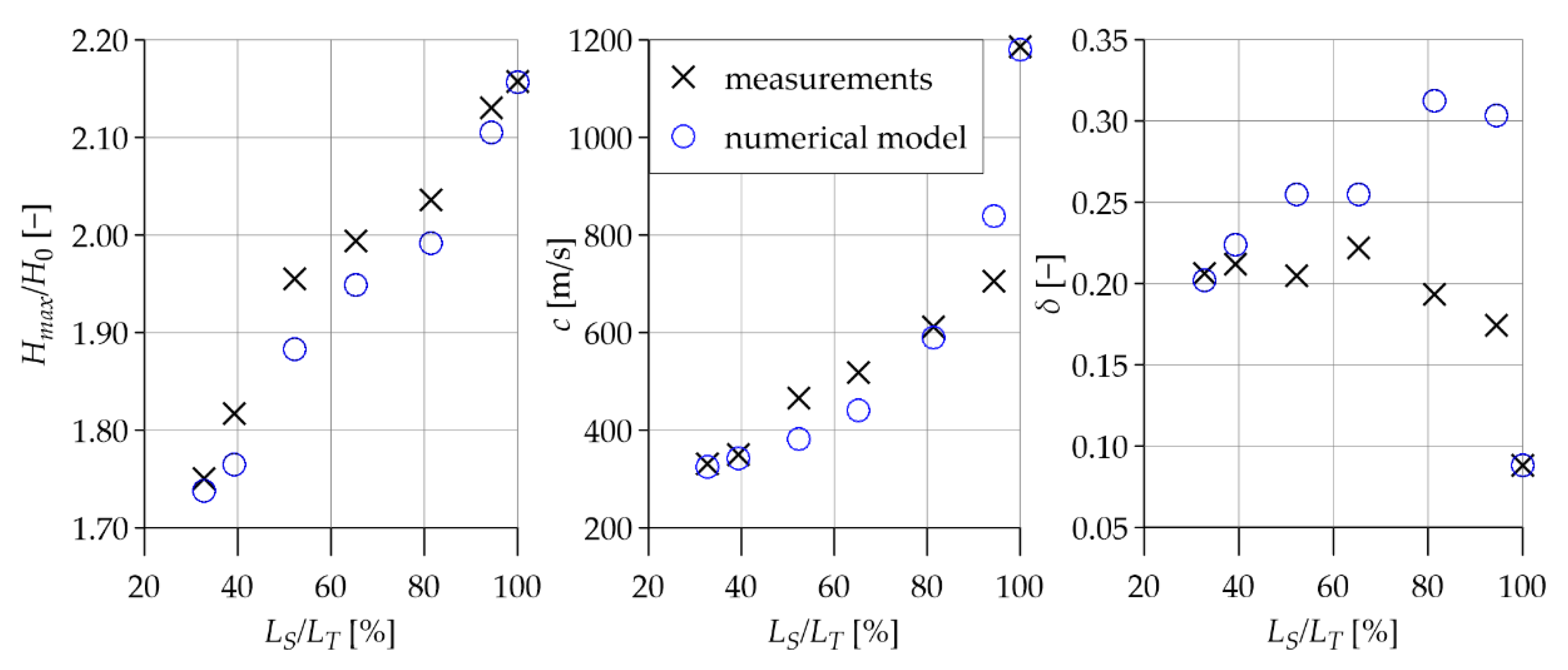
In order to assess the compliance between simulated and measured pressure oscillations, the pressure wave parameters used earlier (dimensionless pressure increase, mean pressure wave velocity, and the logarithmic damping decrement), calculated for both experimental and numerical data, are compiled in Figure 11.
Comparison of the pressure wave parameters shown in Figure 11 confirms the conclusions drawn from the visual analysis of simulated and observed pressure signals. It should be noted that, in all cases, values of the dimensionless pressure increase obtained on the basis of experimental data are similar, although slightly lower than those obtained with the use of the numerical model. Figure 11 also shows that, as the LS/LT ratio increases, the mean velocity of the pressure wave increases at a different rate for the calculated and observed H(t) curves. The greatest discrepancy can be seen in the logarithmic damping decrement. Figure 11 illustrates the opposite trend of the change of δ with the increase in the length of the steel section. As expected, experimental data indicate that as the LS/LT ratio increases, the pressure wave decays slower. However, pressure oscillations calculated for steel-pipeline systems tend to attenuate faster with the increase in the LS/LT ratio. This indicates that the calibrated values of creep compliance and retardation time which referred to the system with the longest plastic section are overestimated in terms of describing a transient response in higher-frequency pipeline systems. The obtained results show that calibrated creep parameters do not have any global character. Any alteration in the pipeline system (e.g., shortening or lengthening of the plastic section in multi-pipe system) requires these parameters to be recalibrated.
6. Conclusions
In this study, the water hammer phenomenon in serially connected steel and HDPE pipes with different inner diameters was analyzed from both an experimental and a numerical point of view. Laboratory tests were conducted on a simple tank–pipeline–valve model and included different configurations of lengths of each pipe. The collected transient data revealed that the maximum pressure increase linearly depended on the share of the steel section in the total pipeline length. Despite the significantly smaller diameter of the HDPE pipe compared to the steel pipe, introducing an in-line plastic section into the pipeline system suppressed the valve-induced pressure surges.
In order to numerically simulate experimental water hammer events, a transient solver which made it possible to take into account unsteady friction and the viscoelastic behavior of the pipe wall was used. The combination of Brunone-Vitkovský IAB model applied to the steel section and the one-element Kelvin–Voigt model accounting for the viscoelastic properties of the HDPE pipe made it possible to obtain satisfactory agreement between the calculated and measured pressure signals.
Numerical parameters calibrated on a single pipeline system were introduced in a numerical model to simulate the water hammer in different configurations of lengths of steel and HDPE sections. It was demonstrated that this approach fails to reproduce the observed H(t) curve for a pipeline system with significantly different lengths of each section. From a practical standpoint, any change in the configuration of the pipeline system causes requires the creep parameters to be recalibrated.
This research has raised many questions in need of further investigation. Future work will concentrate on the performance of the WFB model of unsteady friction in numerical models simulating the water hammer in steel–plastic pipeline systems. Moreover, the influence of applying a different number of Kelvin–Voigt elements on simulating hydraulic transients in multi-pipe systems will be examined.
Author Contributions
Conceptualization, M.K. and A.K.; methodology, M.K., A.K., and A.M.; software, M.K. and K.U.; validation, M.K.; formal analysis, M.K., K.U., and A.M.; investigation, M.K. and K.U.; resources, M.K., A.K., and K.U.; writing—original draft preparation, M.K.; writing—review and editing, A.K., K.U., and A.M.; visualization, M.K.; supervision, M.K.; project administration, M.K.; funding acquisition, M.K. All authors have read and agreed to the published version of the manuscript.
Funding
This work was supported by the Faculty of Building Services, Hydro and Environmental Engineering, Warsaw University of Technology (Grant no. 504/04608).
Data Availability Statement
The code generated during the study and experimental data are available from the corresponding author by request.
Conflicts of Interest
The authors declare no conflict of interest.
Abbreviations
| Nomenclature | |
| A | cross-sectional area of water stream (m2) |
| c | pressure wave velocity (m/s) |
| D | pipe internal diameter (m) |
| E0 | elastic bulk modulus of the spring (Pa) |
| Ek | elastic bulk modulus of the k-th Kelvin–Voigt element (Pa) |
| f | friction factor (−) |
| g | gravity acceleration (m/s2) |
| H | pressure head (m) |
| ΔHmax | maximum pressure head increase (m) |
| J0 | instantaneous creep compliance (Pa−1) |
| Jk | creep compliance of the k-th Kelvin–Voigt element (Pa−1) |
| K | bulk modulus of elasticity of the liquid (Pa) |
| kV | unsteady friction coefficient (−) |
| L | length of the individual pipe section (m) |
| m | the number of the first pressure peak taken into account to calculate logarithmic damping decrement (−) |
| n | the number of subsequent pressure peaks used to calculate damping decrement (−) |
| N | total number of Kelvin–Voigt elements (−) |
| Q | volumetric flow rate (m3/s) |
| s | pipe-wall thickness (m) |
| t | time (s) |
| tc | valve closing time (s) |
| V | mean flow velocity (m/s) |
| X | space coordinate (m) |
| Δt | time interval (s) |
| Δx | space interval (m) |
| α | parameter dependent on pipe diameter and constraints (−) |
| γ | volumetric weight of the fluid (kg/m3) |
| δ | logarithmic damping decrement (−) |
| ε0 | instantaneous (elastic) strain (−) |
| ερ | retarded strain (−) |
| θ | relaxation coefficient for flow-time derivative calculation in IAB model numerical scheme (−) |
| μκ | viscosity of the k-th dashpot (kg/sm) |
| τκ | the retardation time of k-th Kelvin–Voigt element (s) |
| Acronyms | |
| IAB | instantaneous acceleration-based model of unsteady friction |
| HDPE | high-density polyethylene |
| WFB | weighting function-based model of unsteady friction |
| Subscripts | |
| i | number of computational node |
| k | number of Kelvin–Voigt element |
| S | steel section |
| P | HDPE section |
| 0 | steady-state flow parameter |
References
- Wylie, E.B.; Streeter, V.L.; Suo, L. Fluid Transients in Systems; Prentice Hall, Prentice-Hall International: Upper Saddle River, NJ, USA; London, UK, 1997; ISBN 978-0-13-934423-7. [Google Scholar]
- Chaudhry, M.H. Applied Hydraulic Transients; Springer: New York, NY, USA, 2014; ISBN 978-1-4614-8538-4. [Google Scholar]
- Gong, J.; Stephens, M.L.; Lambert, M.F.; Zecchin, A.C.; Simpson, A.R. Pressure Surge Suppression Using a Metallic-Plastic-Metallic Pipe Configuration. J. Hydraul. Eng. 2018, 144, 04018025. [Google Scholar] [CrossRef]
- Garg, R.K.; Kumar, A. Experimental and Numerical Investigations of Water Hammer Analysis in Pipeline with Two Different Materials and Their Combined Configuration. Int. J. Pres. Ves. Pip. 2020, 188, 104219. [Google Scholar] [CrossRef]
- Triki, A. Water-Hammer Control in Pressurized-Pipe Flow Using an in-Line Polymeric Short-Section. Acta Mech. 2016, 227, 777–793. [Google Scholar] [CrossRef]
- Ferrante, M. Transients in a Series of Two Polymeric Pipes of Different Materials. J. Hydraul. Res. 2021, 59, 810–819. [Google Scholar] [CrossRef]
- Bettaieb, N.; Guidara, M.A.; Haj Taieb, E. Impact of Metallic-Plastic Pipe Configurations on Transient Pressure Response in Branched WDN. Int. J. Pres. Ves. Pip. 2020, 188, 104204. [Google Scholar] [CrossRef]
- Parmakian, J. Waterhammer Analysis; Prentice Hall: New York, NY, USA, 1955. [Google Scholar]
- Landry, C.; Nicolet, C.; Bergant, A.; Müller, A.; Avellan, F. Modeling of Unsteady Friction and Viscoelastic Damping in Piping Systems. IOP Conf. Ser. Earth Environ. Sci. 2012, 15, 052030. [Google Scholar] [CrossRef]
- Zielke, W. Frequency-Dependent Friction in Transient Pipe Flow. J. Basic Eng. 1968, 90, 109–115. [Google Scholar] [CrossRef]
- Vardy, A.E.; Brown, J.M.B. Transient, Turbulent, Smooth Pipe Friction. J. Hydraul. Res. 1995, 33, 435–456. [Google Scholar] [CrossRef]
- Vardy, A.E.; Brown, J.M.B. Transient Turbulent Friction in Fully Rough Pipe Flows. J. Sound Vib. 2004, 270, 233–257. [Google Scholar] [CrossRef]
- Brunone, B.; Golia, U.M.; Greco, M. Effects of Two-Dimensionality on Pipe Transients Modeling. J. Hydraul. 1995, 121, 906–912. [Google Scholar] [CrossRef]
- Brunone, B.; Golia, U.M. Discussion of “Systematic Evaluation of One-Dimensional Unsteady Friction Models in Simple Pipelines” by J. P. Vitkovsky, A. Bergant, A. R. Simpson, and M. F. Lambert. J. Hydraul. Eng. 2008, 134, 282–284. [Google Scholar] [CrossRef]
- Vítkovský, J.P.; Bergant, A.; Simpson, A.R.; Lambert, M.F. Systematic Evaluation of One-Dimensional Unsteady Friction Models in Simple Pipelines. J. Hydraul. Eng. 2006, 132, 696–708. [Google Scholar] [CrossRef] [Green Version]
- Abdeldayem, O.; Ferràs, D.; van der Zwan, S.; Kennedy, M. Analysis of Unsteady Friction Models Used in Engineering Software for Water Hammer Analysis: Implementation Case in WANDA. Water 2021, 13, 495. [Google Scholar] [CrossRef]
- Bergant, A.; Ross Simpson, A.; Vìtkovsky, J. Developments in Unsteady Pipe Flow Friction Modelling. J. Hydraul. Res. 2001, 39, 249–257. [Google Scholar] [CrossRef] [Green Version]
- Vardy, A.E.; Brown, J.M.B. Transient turbulent friction in smooth pipe flows. J. Sound Vib. 2003, 259, 1011–1036. [Google Scholar] [CrossRef]
- Ghidaoui, M.S.; Zhao, M.; McInnis, D.A.; Axworthy, D.H. A Review of Water Hammer Theory and Practice. App. Mech. Rev. 2005, 58, 49–76. [Google Scholar] [CrossRef] [Green Version]
- Shaw, M.T. Introduction to Polymer Viscoelasticity, 4th ed.; Wiley: Hoboken, NJ, USA, 2018; ISBN 978-1-119-18182-8. [Google Scholar]
- Keramat, A.; Tijsseling, A.S.; Hou, Q.; Ahmadi, A. Fluid–Structure Interaction with Pipe-Wall Viscoelasticity during Water Hammer. J. Fluid. Struct. 2012, 28, 434–455. [Google Scholar] [CrossRef] [Green Version]
- Pezzinga, G.; Scandura, P. Unsteady Flow in Installations with Polymeric Additional Pipe. J. Hydraul. 1995, 121, 802–811. [Google Scholar] [CrossRef]
- Covas, D.; Stoianov, I.; Mano, J.F.; Ramos, H.; Graham, N.; Maksimovic, C. The Dynamic Effect of Pipe-Wall Viscoelasticity in Hydraulic Transients. Part II—Model Development, Calibration and Verification. J. Hydraul. Res. 2005, 43, 56–70. [Google Scholar] [CrossRef]
- Covas, D.; Stoianov, I.; Ramos, H.; Graham, N.; Maksimovic, C. The Dynamic Effect of Pipe-Wall Viscoelasticity in Hydraulic Transients. Part I—Experimental Analysis and Creep Characterization. J. Hydraul. Res. 2004, 42, 517–532. [Google Scholar] [CrossRef]
- Weinerowska-Bords, K. Viscoelastic Model of Waterhammer in Single Pipeline – Problems and Questions. Archives Hydro-Eng. Environ. Mech. 2006, 53, 21. [Google Scholar]
- Pezzinga, G.; Brunone, B.; Cannizzaro, D.; Ferrante, M.; Meniconi, S.; Berni, A. Two-Dimensional Features of Viscoelastic Models of Pipe Transients. J. Hydraul. Eng. 2014, 140, 04014036. [Google Scholar] [CrossRef]
- Pezzinga, G.; Brunone, B.; Meniconi, S. Relevance of Pipe Period on Kelvin-Voigt Viscoelastic Parameters: 1D and 2D Inverse Transient Analysis. J. Hydraul. Eng. 2016, 142, 04016063. [Google Scholar] [CrossRef]
- Sun, Q.; Zhang, Z.; Wu, Y.; Xu, Y.; Liang, H. Numerical Analysis of Transient Pressure Damping in Viscoelastic Pipes at Different Water Temperatures. Materials 2022, 15, 4904. [Google Scholar] [CrossRef] [PubMed]
- Meniconi, S.; Brunone, B.; Ferrante, M. Water-Hammer Pressure Waves Interaction at Cross-Section Changes in Series in Viscoelastic Pipes. J. Fluid. Struct. 2012, 33, 44–58. [Google Scholar] [CrossRef]
- Kubrak, M.; Malesińska, A.; Kodura, A.; Urbanowicz, K.; Stosiak, M. Hydraulic Transients in Viscoelastic Pipeline System with Sudden Cross-Section Changes. Energies 2021, 14, 4071. [Google Scholar] [CrossRef]
- Malesinska, A.; Kubrak, M.; Rogulski, M.; Puntorieri, P.; Fiamma, V.; Barbaro, G. Water Hammer Simulation in a Steel Pipeline System with a Sudden Cross-Section Change. J. Fluid. Eng. 2021, 143, 091204. [Google Scholar] [CrossRef]
- Keramat, A.; Haghighi, A. Straightforward Transient-Based Approach for the Creep Function Determination in Viscoelastic Pipes. J. Hydraul. Eng. 2014, 140, 04014058. [Google Scholar] [CrossRef]
- Tijsseling, A.S.; Vardy, A.E. What Is Wave Speed? In Proceedings of the 12th International Conference on Pressure Surges, Dublin, Ireland, 18–20 November 2015; pp. 343–360. [Google Scholar]
- Adamkowski, A.; Henclik, S.; Janicki, W.; Lewandowski, M. The Influence of Pipeline Supports Stiffness onto the Water Hammer Run. Eur. J. Mech.-B/Fluid. 2017, 61, 297–303. [Google Scholar] [CrossRef] [Green Version]
- Soares, A.K.; Covas, D.I.; Reis, L.F. Analysis of PVC Pipe-Wall Viscoelasticity during Water Hammer. J. Hydraul. Eng. 2008, 134, 1389–1394. [Google Scholar] [CrossRef]
- Covas, D. Inverse Transient Analysis for Leak Detection and Calibration of Water Pipe Systems—Modelling Special Dynamic Effects. Ph.D. Thesis, University of London, London, UK, 2003. [Google Scholar]
- Sarker, S.; Sarker, T. Spectral Properties of Water Hammer Wave. App. Mech. 2022, 3, 799–814. [Google Scholar] [CrossRef]
- Weinerowska-Bords, K. Alternative Approach to Convolution Term of Viscoelasticity in Equations of Unsteady Pipe Flow. J. Fluid. Eng. 2015, 137, 054501. [Google Scholar] [CrossRef]
- Soares, A.K.; Covas, D.I.C.; Reis, L.F.R. Leak Detection by Inverse Transient Analysis in an Experimental PVC Pipe System. J. Hydroinformatics 2011, 13, 153–166. [Google Scholar] [CrossRef]
- Duan, H.-F.; Ghidaoui, M.; Lee, P.J.; Tung, Y.-K. Unsteady Friction and Visco-Elasticity in Pipe Fluid Transients. J. Hydrau. Res. 2010, 48, 354–362. [Google Scholar] [CrossRef]
- Mitosek, M.; Chorzelski, M. Influence of Visco-Elasticity on Pressure Wave Velocity in Polyethylene MDPE Pipe. Archives Hydro-Eng. Environ. Mech. 2003, 50, 127–140. [Google Scholar]
Figure 1.
Generalized Kelvin–Voigt model.

Figure 2.
Laboratory setup: 1—pressure tank; 2—Bourdon pressure gauge; 3—water supply system; 4—pressure sensor; 5—valve initiating water hammer; 6—inductive flowmeter; 7—regulating valve; 8—data logger; 9—laptop; LS—length of the steel section (m); LP—length of the plastic (HDPE) section (m); LT—total length of the pipeline system (m).

Figure 3.
Comparison between experimental transient data: (a) System #1 vs. system #2; (b) System #2 vs. system #3; (c) System #3 vs. system #4; (d) System #4 vs. system #5; (e) System #5 vs. system #6; and (f) System #6 vs. system #7.
Figure 3.
Comparison between experimental transient data: (a) System #1 vs. system #2; (b) System #2 vs. system #3; (c) System #3 vs. system #4; (d) System #4 vs. system #5; (e) System #5 vs. system #6; and (f) System #6 vs. system #7.

Figure 4.
First phase of pressure oscillations registered during all water hammer runs.

Figure 5.
Values of dimensionless maximum pressure increase as a function of LS/LT.

Figure 6.
Values of mean pressure wave velocities in tested systems as a function of LS/LT.

Figure 7.
Values of logarithmic damping decrement as a function of LS/LT.

Figure 8.
Numerical grid in fixed-grid method of characteristics.

Figure 9.
Comparison between calculated and measured pressure oscillations: (a) Unsteady friction coefficient calculated using Equations (5) and (7); and (b) Calibrated unsteady friction coefficient.
Figure 9.
Comparison between calculated and measured pressure oscillations: (a) Unsteady friction coefficient calculated using Equations (5) and (7); and (b) Calibrated unsteady friction coefficient.

Figure 10.
Comparison between calculated and measured pressure oscillations: (a) System #1; (b) System #2; (c) System #3; (d) System #4; (e) System #5; and (f) System #6.
Figure 10.
Comparison between calculated and measured pressure oscillations: (a) System #1; (b) System #2; (c) System #3; (d) System #4; (e) System #5; and (f) System #6.

Figure 11.
Comparison between calculated and measured values of the dimensionless pressure increase, mean pressure wave velocity, and the logarithmic damping decrement.
Figure 11.
Comparison between calculated and measured values of the dimensionless pressure increase, mean pressure wave velocity, and the logarithmic damping decrement.


Table 1.
Dimensions of the pipeline system in each configuration and steady state flow parameters.
| System Config. | LS (m) | LP (m) | LT (m) | LS/LT (%) | V0S (m/s) | V0P (m/s) |
|---|---|---|---|---|---|---|
| #1 | 15.75 | 32.35 | 48.10 | 33 | 0.43 | 0.97 |
| #2 | 18.90 | 29.20 | 48.10 | 39 | 0.42 | 0.95 |
| #3 | 25.15 | 22.95 | 48.10 | 52 | 0.41 | 0.93 |
| #4 | 31.40 | 16.70 | 48.10 | 65 | 0.41 | 0.93 |
| #5 | 39.15 | 8.95 | 48.10 | 81 | 0.42 | 0.95 |
| #6 | 45.40 | 2.70 | 48.10 | 94 | 0.41 | 0.93 |
| #7 | 48.10 | 0.00 | 48.10 | 100 | 0.42 | 0.95 |
Note: where V0S—initial steady flow velocity in the steel pipe (m/s); V0P—initial steady flow velocity in the HDPE pipe (m/s).
Table 2.
Coefficients CN, Ca+, CP, and C a− are used to model each section of the pipeline.
| Steel Section | |
| (21) | |
| (22) | |
| (23) | |
| (24) | |
| HDPE Section | |
| (25) | |
| (26) | |
| (27) | |
| , | (28) |
Publisher’s Note: MDPI stays neutral with regard to jurisdictional claims in published maps and institutional affiliations. |
© 2022 by the authors. Licensee MDPI, Basel, Switzerland. This article is an open access article distributed under the terms and conditions of the Creative Commons Attribution (CC BY) license (https://creativecommons.org/licenses/by/4.0/).
Share and Cite
MDPI and ACS Style
Kubrak, M.; Kodura, A.; Malesińska, A.; Urbanowicz, K. Water Hammer in Steel–Plastic Pipes Connected in Series. Water 2022, 14, 3107. https://doi.org/10.3390/w14193107
AMA Style
Kubrak M, Kodura A, Malesińska A, Urbanowicz K. Water Hammer in Steel–Plastic Pipes Connected in Series. Water. 2022; 14(19):3107. https://doi.org/10.3390/w14193107
Chicago/Turabian StyleKubrak, Michał, Apoloniusz Kodura, Agnieszka Malesińska, and Kamil Urbanowicz. 2022. "Water Hammer in Steel–Plastic Pipes Connected in Series" Water 14, no. 19: 3107. https://doi.org/10.3390/w14193107
Note that from the first issue of 2016, this journal uses article numbers instead of page numbers. See further details here.