
Smooth and Stepped Converging Spillway Modeling Using the SPH Method


1
School of Civil and Environmental Engineering, Federal University of Goiás, Goiânia 74605-220, GO, Brazil
2
Civil Engineering Research and Innovation for Sustainability, Instituto Superior Técnico, Universidade de Lisboa, 1049-001 Lisbon, Portugal
3
Department of Hydraulics and Sanitation, São Carlos School of Engineering, University of São Paulo, São Carlos 13566-590, SP, Brazil
4
Hydro Engineering Solutions, Auburn, AL 36830, USA
5
Bentley Systems, 1990-208 Lisbon, Portugal
*
Author to whom correspondence should be addressed.
Water 2022, 14(19), 3103; https://doi.org/10.3390/w14193103
Submission received: 6 August 2022
/
Revised: 23 September 2022
/
Accepted: 26 September 2022
/
Published: 2 October 2022
(This article belongs to the Special Issue Advances in Spillway Hydraulics: From Theory to Practice)
Abstract
:Three-dimensional (3D) simulations using the smoothed particle hydrodynamics (SPH) method were performed for smooth and stepped spillways with converging walls, in order to evaluate the influence of the wall deflection and the step macro-roughness on the main non-aerated flow properties. The simulations encompassed a 1V:2H sloping spillway, wall convergence angles of 9.9° and 19.3°, and discharges corresponding to skimming flow regime, in the stepped chute. The overall development of the experimental data on flow depths, velocity profiles, and standing wave widths was generally well predicted by the numerical simulations. However, larger deviations in flow depths and velocities were observed close to the upstream end of the chute and close to the pseudo-bottom of the stepped invert, respectively. The results showed that the height and width of the standing waves were significantly influenced by the wall convergence angle and by the macro-roughness of the invert, increasing with a larger wall deflection, and attenuated on the stepped chute. The numerical velocity and vorticity fields, along with the 3D recirculating vortices on the stepped invert, were in line with recent findings on constant width chutes.
1. Introduction
Converging transitions along discharge channels, i.e., having a terminal structure narrower than the crest, may be imposed by site or economy constraints [1]. In light of the scenarios of climate change and urbanization, converging transitions have also been applied in dam rehabilitation projects to increase the discharge capacity of spillways, by extending the spillway crest width [2,3].
A larger crest width presents the advantage of reducing the hydraulic head over the crest, and thus the pressure over the slab for identical discharge [4]. However, the adverse effects of the wall deflection on channels with supercritical flows comprise the occurrence of oblique standing waves, also named oblique hydraulic jumps or oblique shock waves [5,6]. Therefore, in converging chutes, special attention should be given to the design of training walls in order to prevent wave run-up, because of the significant increase in the flow depths near the walls [1,5]. Besides, concerns may arise with the efficiency of the energy dissipation in the stilling basin at the toe of the dam [3,7].
Pioneering research conducted in the 1940s and 1950s on horizontal channels with lateral contraction was carried out by [4,5,8,9], among others. Their experimental investigations and theoretical developments, including the application of the method of characteristics, were relevant for understanding the wave patterns for a range of Froude numbers and the establishment of design criteria in order to reduce or even eliminate the standing waves. More recent experimental research concerned the evaluation of shock surfaces [6], velocity profiles and/or turbulent kinetic energy [6,10], along with wave diffractors [11,12]. Numerical simulations were also undertaken by solving the two-dimensional shallow-water equations [6,13,14,15,16] or the three-dimensional Reynolds-averaged Navier–Stokes equations [16]. Investigations addressing inclined chute contractions were also carried out, as presented by [12,17,18], determining the role of the bottom slope on the flow patterns of the standing waves.
A summary of investigations addressing stepped spillways with converging walls is presented in Table 1 [2,7,19,20,21,22,23,24,25,26,27,28], comprising experimental data for a broad range of experimental flow conditions, such as wall convergence angles, inflow Froude numbers, and step heights. Additionally, the author of [24] developed a theoretical relationship to determine the flow depths at the training wall, based on a simplified momentum analysis approach, which was later improved by the authors of [29], by including the weight force associated with the control volume used in their analysis. The influence of the air entrainment on the standing wave characteristics was discussed in [7]. There, the primary wave was considered as the non-aerated region of the wave, which steadily reduced downstream of the inception point. The secondary wave was defined as the fully aerated region that formed and increased downstream of the inception point.
Few numerical studies simulating the flow over converging spillways are available to date, for smooth conventional chutes (e.g., [30,31,32,33]) or stepped chutes (e.g., [31,32]). Their results comprise mainly the analysis of flow depths, velocity profiles, pressure distributions, and the evolution of the standing wave width along the spillway. Among the mentioned studies, the Lagrangian particle finite element method (PFEM) was used in [33] to simulate the flow over two converging dam spillways, showing the ability of the meshless based method to address problems involving high irregularities in the free surface.
To the best of the authors’ knowledge, applications using the meshless smoothed particle hydrodynamics (SPH) method for studying the effect of the wall convergence on the flow characteristics were not developed until recently. Therefore, the aim of the present study was to simulate the non-aerated flow over a 1V:2H sloping spillway with converging walls of 9.9° and 19.3° for smooth and stepped inverts (for skimming flow regime) using the SPH method, and to compare the results with the corresponding experimental values previously acquired in the framework of [21,23]. The discussion of the numerical results focusses on the prediction of the flow depth development at the chute walls and centerline, the centerline velocity profiles, and the development of the standing wave width. Numerical results for the cross-sectional flow depth profiles, velocity, and vorticity contour fields are also presented and analyzed.
2. Materials and Methods
2.1. Experimental Setup
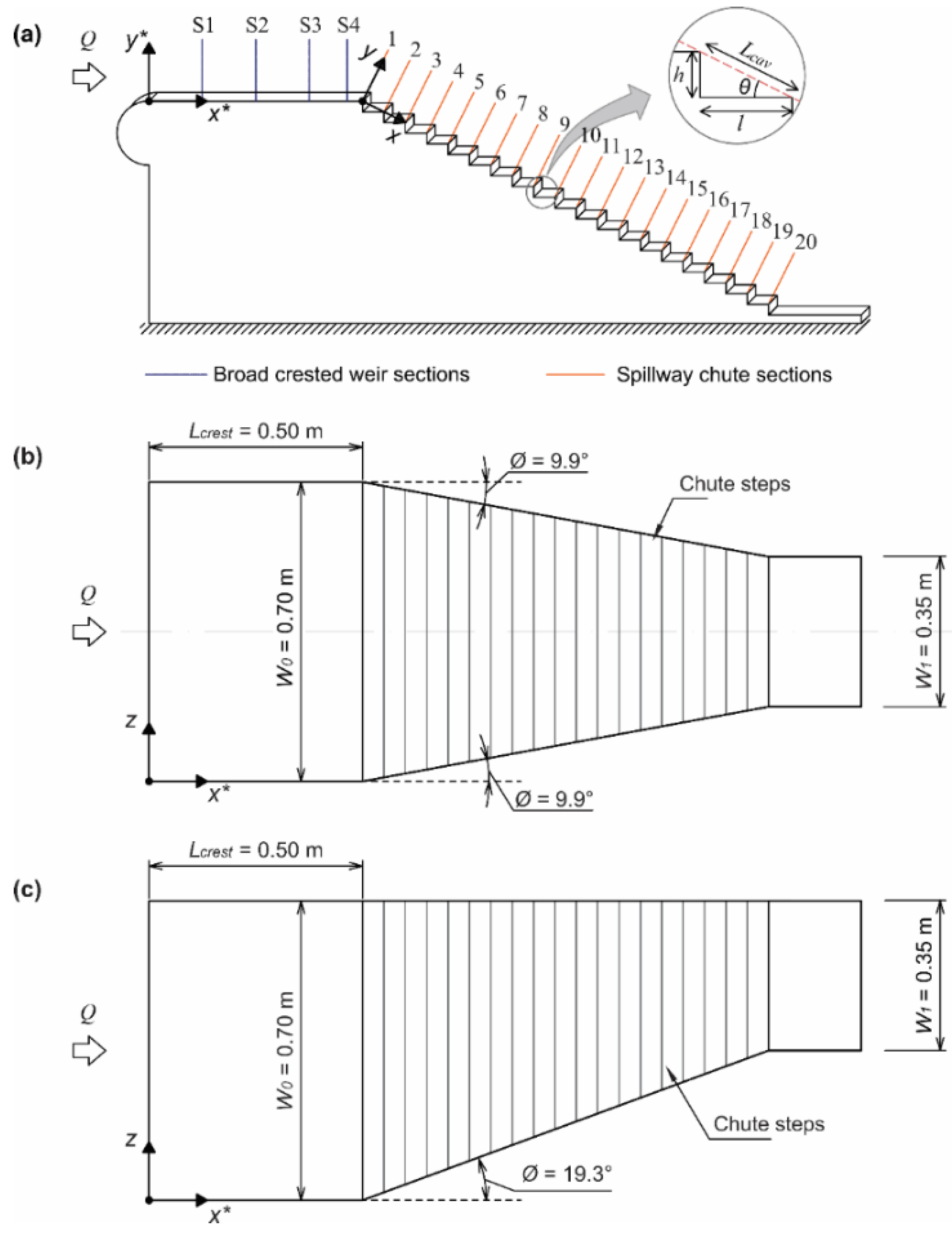
The experimental data obtained in [21,23] were used for validation of the numerical simulations presented herein. The experiments were carried out in an experimental facility assembled at the Hydraulic and Water Resources Laboratory of the Instituto Superior Técnico, University of Lisbon, Portugal. The facility encompassed an 8.0 m long and 0.7 m wide rectangular flume with Plexiglas walls, with a water recirculation system. The physical spillway model consisted of a 0.5 m high, 0.7 m wide, and 0.5 m long uncontrolled broad crested weir, followed by a smooth or stepped chute with a slope of 1V:2H (chute angle from the horizontal = 26.6°) and a stilling basin. The stepped configuration comprised 20 steps of 2.5 cm height () each. The upstream width of the chute was = 0.7 m, linearly reducing to the downstream width of = 0.35 m (Figure 1), by means of (i) one converging wall of = 19.3° [21] and (ii) two converging walls of = 9.9° [23].
The tested discharges () were 35, 42, 49, and 56 L/s, yielding approach unit discharges () of 50, 60, 70, and 80 L/(s m) considering the upstream chute width = 0.7 m. The corresponding critical flow depths () were 0.063, 0.072, 0.079, and 0.087 m, and the critical flow depths normalized by the step height () were 2.52, 2.88, 3.16, and 3.48, respectively. The approach shock number () ranged from 0.31 to 0.32 for the wall convergence angle = 9.9°, and from 0.60 to 0.63 for = 19.3°. In the above formula, is given in radians and is the approach Froude number (), which depends on the approach flow depth at the chute centerline immediately upstream of the wall deflection at = 0 (), where is the streamwise coordinate along the chute (Figure 1).
All tests corresponded to clear water flow on the smooth chute and to skimming flow on the stepped chute. On the latter setup, the inception of air entrainment was visually observed only for = 35 L/s at the 15th step ( = 0.78 m), irrespective of the studied wall convergence angle, i.e., = 9.9° [23] or = 19.3° [21].
The flow depths and velocities were determined at four cross sections along the broad crested weir ( = 0.125, 0.250, 0.375, and 0.464 m) and at locations corresponding to the step edges along the spillway, perpendicularly to the invert, as shown in Figure 1. The measurement of flow velocity was carried out using a Prandtl–Pitot tube with an external diameter of 8 mm, connected to a manometer [21,23]. A total pressure probe with an external diameter of 1 mm connected to a manometer was also used in [23] for velocity measurements along the broad crested weir.
The flow depths along the centerline of the broad crested weir, as well as along the spillway centerline (on the chute with = 9.9°) or near the non-converging wall (i.e., pseudo-centerline, on the chute with = 19.3°), were determined using a point gauge, with 0.05 mm resolution. The flow depths at the flume walls were obtained using 1 mm graduation rulers positioned perpendicularly to the bottom or to the pseudo-bottom [21,23]. It should be noted that, owing to free surface fluctuations, the uncertainties in the flow depth estimation, namely at the flume walls, are greater than those indicated by the instrumentation resolution, with values ranging from 1.0 mm, for the smallest flow rate, on the smooth chute, up to 5.0 mm, for the largest flow rate, near the downstream end of the stepped chute.
The standing wave width was visually determined in [21,23], using a graduated ruler. A micro-propeller current meter connected to a displacement structure was also used in [23] to measure the standing wave width for the setup with two converging walls of 9.9°. Moving the micro-propeller current meter in the transverse direction, slightly above the free surface in a region unaffected by the standing wave towards the converging wall, the standing wave front was considered as the transverse position where the device started continuously spinning with the flow. The experimental widths presented herein are the mean values measured on the left and right flume walls for = 9.9°, or on the right flume wall for = 19.3°. Considering the range of discharges adopted in the experiments, the standing waves did not appear to reach the symmetry line of the spillway for = 9.9° or the non-converging wall for = 19.3°.
The measurement of the standing wave width using the micro-propeller current meter was only possible upstream of the inception point, as the free surface was very irregular downstream of this position owing to the air entrainment and increased flow turbulence. Downstream of the inception point, larger uncertainties resulting from visual observations were also expected because of the standing wave oscillations [23]. More details about the instrumentation and the experimental procedure can be found in [21,23,34].
2.2. Numerical Simulations
The numerical simulations were developed for smooth and stepped spillways (with a step height of 2.5 cm), using a prototype scale of 10:1 (numerical model/experimental model) and Froude law similitude. Similar scale factors were previously adopted, namely, 10:1 [34], 15:1 [35], and 10:1 [36]. In the present study, scale effects are expected to be negligible, because it focusses on the non-aerated flow region, with flow depths over the broad crested weir generally greater than 0.06 m and Reynolds numbers (, where is the mean flow velocity, is the hydraulic radius and is the kinematic viscosity of water), satisfying the condition > 104.5 [37].
The DualSPHysics software, a weakly compressible SPH Navier–Stokes solver, was used to perform the three-dimensional (3D) simulations. A brief summary of the equations used in the SPH method is presented herein, based on [38,39,40].
The properties of the discrete particles representing the fluid are determined from the convolution of a smoothing kernel function () and a function over an influenced domain, as represented by Equation (1). The Wendland kernel function used in the present study is described in Equation (2) [41].
where is the position vector; a, b = subscripts referring to the interpolating particle a and the neighboring particles b; = smoothing kernel function; , = mass and density of the b-th particle, respectively; = kernel function length; in 3D; and is the normalized particle spacing in relation to the kernel function length.
The SPH method comprehends the solution of the discrete forms of the continuity and momentum equations, expressed by Equations (3) and (4), respectively, and the solution of the equation of state for a weak compressible fluid, which couples the pressure with the fluid density (Equation (5)).
where t = time; = velocity vector; ; = gradient of the kernel function; ; = numerical density diffusion term, artificially introduced to reduce fluid density fluctuations; = pressure; = gravity acceleration; = dissipation terms; = 1000 kg/m3 is the reference density; = numerical speed of sound defined as ; and γ = 7 is the exponent of the equation of state for water.
The numerical density diffusion term and the dissipation term in Equations (3) and (4) adopted herein were the Delta-SPH term proposed by [42] and the sub-particle scale (SPS) model, which considers the effects of laminar and turbulent viscosity [39,43], given by Equations (6) and (7), respectively.
where δ = a coefficient that defines the magnitude of the Delta-SPH term, adopted herein as 0.1, as recommended for most applications [39]; is the average speed of sound; ; = kinematic viscosity; and = element of the SPS stress tensor .
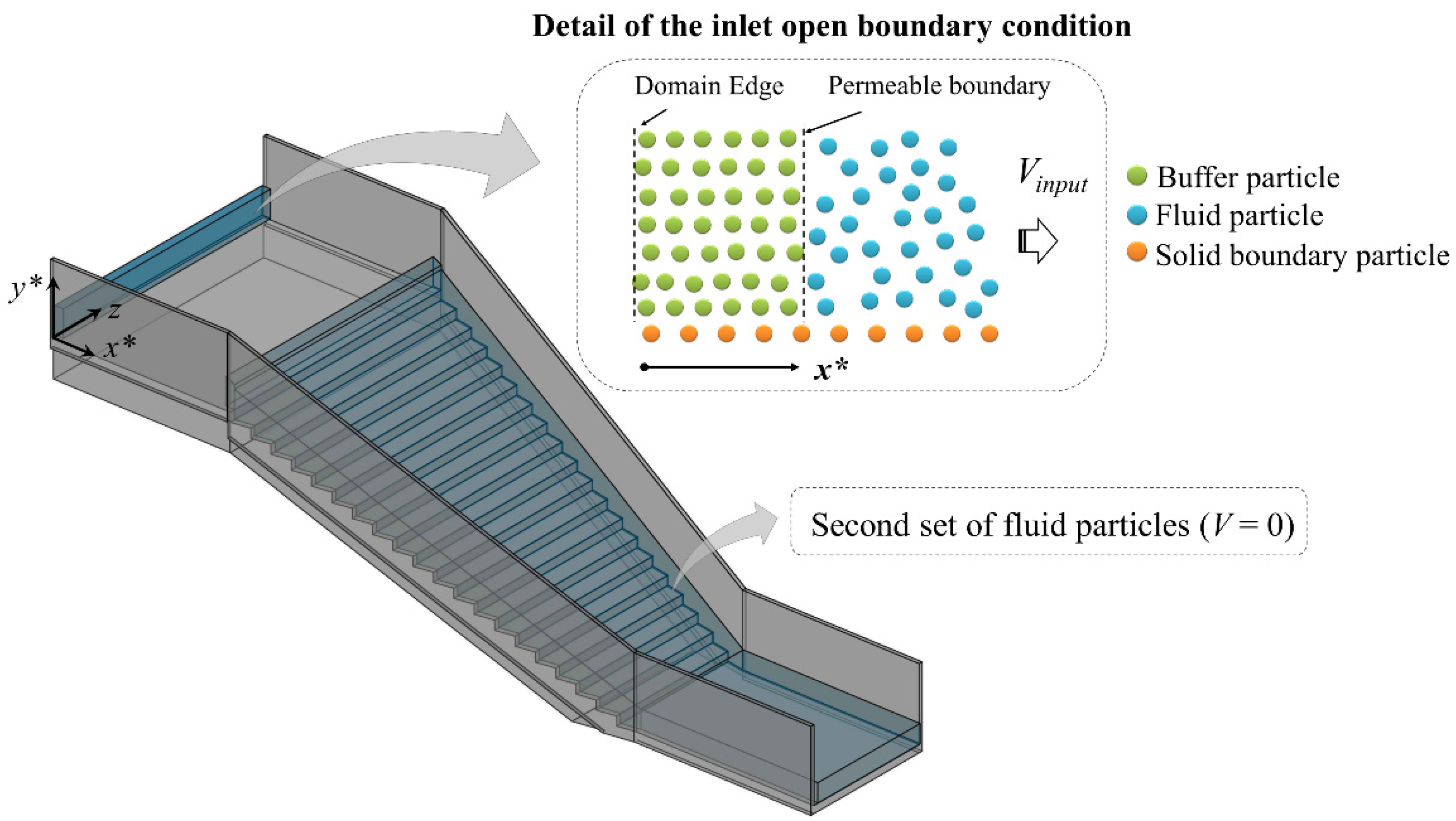
The upstream inlet condition was simulated as an open boundary, using six layers of buffer particles (fictitious SPH particles as described by [40]) at the inlet, which are continuously added into the domain, thus effectively modelling a large upstream reservoir (Figure 2). The height and velocity assigned to these layers were equivalent to the measured flow depth at = 0.125 m, from the upstream end of the broad crested weir, and the experimental free-stream velocity at the referred location, respectively. The chute was also initially filled with fluid particles with null velocity. The solid boundaries of the spillway were assembled using the dynamic boundary conditions (DBCs) implemented in DualSPHysics. In DBC, the density and pressure of the fixed particles representing the solid boundaries are computed using the continuity equation and the equation of state, respectively [40].
The initial particle spacing () of 20 mm (prototype scale) was used in the simulations, leading to a normalized step height in relation to the initial particle spacing () of 12.5. An additional value of dp = 17.5 mm at prototype scale ( = 14.3) was used to simulate the smallest discharge of = 35 L/s over the stepped spillway with two converging walls, in order to evaluate the effects of a slightly smaller, yet computationally feasible, initial particle spacing on the numerical flow depths and velocities. The initial particle spacing used in 3D SPH simulations was considerably greater than those adopted in [34] for two-dimensional (2D) SPH simulations, because of limitations related to computational storage and simulation time. Nevertheless, the adopted value for was of the same order of magnitude as that used in previous studies to simulate the flow over constant width stepped spillways, such as [35,36,44,45,46].
The simulations were carried out during 20 s of computational time, with output intervals of 0.01 s. The analysis of the instantaneous free surface profiles along the broad crested weir showed that the flow depths stabilized after 12 s of simulation time. For this reason, the flow depths and velocity profiles were determined as time-averaged values considering the interval between 12 and 20 s of simulation, similarly to [34].
The numerical flow depths at the converging wall () and outside the standing wave were determined from the cross-sectional flow depth profiles. To determine the flow depths in a region unaffected by the standing wave, mean values were calculated considering the following: (i) flow depths near the centerline for the symmetric spillway of = 9.9° () and (ii) flow depths near the non-converging wall (i.e., pseudo-centerline) for the asymmetric spillway of = 19.3° ().
From the cross-sectional flow depth profiles, the numerical standing wave widths were also determined. The standing wave front was approximated as a vertical line, and its location was defined as the transverse position () corresponding to the half-height of the standing wave, above the flow depth uninfluenced by the converging wall.
3. Results
3.1. Flow Depths and Velocity Profiles along the Broad Crested Weir
The flow depths and velocities along the broad crested weir were analyzed for the condition of two converging walls of = 9.9° and the stepped chute. Similar results are expected for the other setups because of similar height and velocity assigned to the layers with fictitious SPH particles at the inlet boundary (buffer particles). The flow depths over the broad crested weir were reasonably well estimated by the numerical simulations, as observed in Figure 3a, comprising the results from the 3D SPH simulation, for = 35 L/s. In this figure (and in the figures that follow in the text), the values of are in the prototype scale of 10:1 (numerical model/experimental model). For the range of discharges, the absolute percentage difference between the 3D SPH results and the experimental data was limited to 6.6% (Figure 3b). However, the inlet boundary condition, with uniform velocity and constant height assigned to the layers composed of fictitious SPH particles, imposed approximately constant flow depths over an initial reach of the weir ( 0.125 m), which does not accurately reproduce the typical streamline curvature and acceleration of the flow in this region (see, e.g., [47]). Further downstream, the 3D SPH free surface profiles were similar to those obtained from the 2D SPH simulations developed by [34] or those obtained using the Flow-3D software by [31,48] for identical experimental conditions.
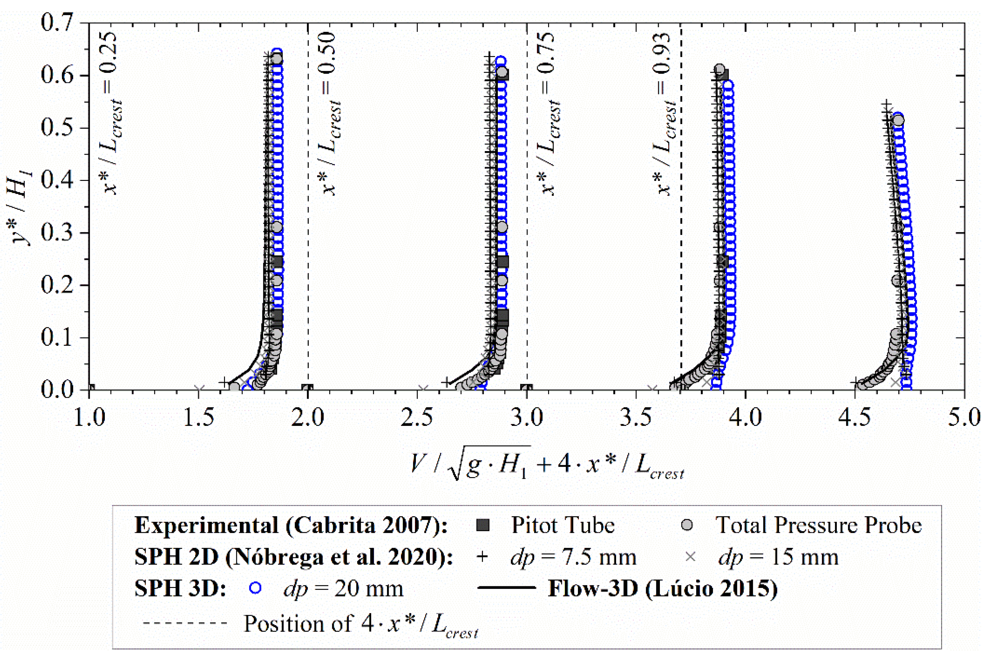
The normalized velocity profiles along the broad crested weir for = 35 L/s are presented in Figure 4, where is the flow velocity, is the upstream total head above the broad crested weir, is the streamwise coordinate along the weir, is the broad crested weir length, and is the normal coordinate perpendicular to the weir bottom (see Figure 1). As observed by the authors of [34], these profiles were not significantly influenced by the initial particle spacing. However, larger deviations can be observed close to the invert for the lower resolutions (i.e., higher values of , = 15 or 20 mm, in 2D or 3D simulations, respectively), particularly near the downstream end of the weir. At each normal cross section, for 0.005 m ( ≥ 0.04), the mean absolute percentage differences between the experimental and the numerical data were lower than 6% and 10%, at = 0.25, 0.50, 0.75, and = 0.93, respectively. Moreover, the dynamic boundary conditions (DBCs) used herein present some limitations, thus affecting the results near the solid boundary. As explained by [40,49], an unphysical gap between the fluid and the solid boundaries appears when fluid approaches the boundary, decreasing the accuracy of calculated pressures at the boundary.
3.2. Flow Depths along the Spillway
3.2.1. Smooth Spillway with Two Converging Walls of = 9.9°
The development of the flow depth along the spillway with two converging walls of = 9.9°, for = 35 L/s, is presented in Figure 5a, whereas the corresponding experimental versus numerical flow depths are included in Figure 6a,c. The flow depth development obtained from 2D SPH simulations, based on the constant width chute [34], along with that estimated by applying the explicit simplified equations developed in [50], are also included in Figure 5a.
For = 35 L/s, a gradual decrease in the flow depth occurs along the smooth spillway centerline (). However, for discharges ranging from 42 L/s to 56 L/s, the flow depths presented nearly constant or gradually increasing values near the downstream end of the chute, as shown in [51] (not shown herein). Even though the standing wave did not appear to reach the centerline of the spillway, a slight increase in the centerline flow depths was noticeable near the downstream end of the chute, similarly to the results of [16], for both 2D depth-averaged and 3D numerical models, using mesh-based methods. In contrast, the flow depths at the converging wall (), for = 9.9°, decreased until 0.4 m and remained almost constant further downstream (Figure 5a).
The overall behavior of the flow depth profiles along the spillway with = 9.9° was reasonably well predicted by the 3D SPH simulations; however, the flow depths at the chute centerline () were in general slightly overestimated. The highest absolute percentage differences for and were generally found at = 0.11 m because of the fluid particles’ detachment upon initially reaching the chute, which was not observed in the experiments. The mean absolute percentage differences were limited to 12% for and 8% for , for 0.22 ≤ (m) ≤ 0.89, considering the range of discharges (Figure 6a,c). The results from the 3D SPH simulations were also in good agreement with the flow depths estimated for constant width chutes, as indicated in Figure 5a, by applying the explicit simplified equation from [50], along with the results attained from 2D SPH simulations, using = 17.5 and 20 mm (present study) or = 7.5 and 15 mm (from [34]).
3.2.2. Smooth Spillway with One Converging Wall of = 19.3°
The development of the flow depth along the spillway with one converging wall of = 19.3°, for = 56 L/s, is presented in Figure 5c, along with the flow depth development obtained from 2D SPH simulations, based on the constant width chute [34] and the flow depth estimated by applying the explicit simplified equations developed by [50]. The corresponding experimental versus numerical flow depths are included in Figure 6a,c.
Considering the range of discharges, the flow depths at the non-converging wall () decreased gradually with distance, as shown in Figure 5c. The flow depths at the converging wall () decreased until approximately 0.4 m and gradually increased downstream of this location.
The general behavior of the flow depth profile at the converging and the non-converging walls along the spillway with = 19.3° was reasonably well predicted by the 3D SPH simulations. The numerical values of the flow depths at the non-converging wall () were in general slightly lower than the experimental data, whereas the numerical flow depths at the converging wall () for = 19.3° generally overestimated the experimental counterparts upstream of 0.4 m, while they slightly underestimated them downstream of this position. The mean absolute percentage differences, for 0.17 ≤ (m) ≤ 0.89 and for the range of discharges, were generally limited to 12% for (measured using the point gauge) and to 9% for (Figure 6a,c). The 3D SPH results at the non-converging wall were also similar to the results obtained from the 2D SPH simulations using = 7.5 mm (from [34]), but on the upstream end of the chute. They were also in agreement with the explicit simplified equation from [50], for constant width chutes.
3.2.3. Stepped Spillway with Two Converging Walls of = 9.9°
The development of the flow depth along the stepped spillway with two converging walls of = 9.9°, for = 35 L/s, is presented in Figure 5b, whereas the related experimental versus numerical flow depths are included in Figure 6b,d. The flow depth development obtained from 2D SPH simulations, based on the constant width chute (e.g., [34]), along with equations developed by [52,53], are also included in Figure 5b.
The experimental flow depths at the stepped spillway centerline () with = 9.9° gradually decreased until 0.40 m, presenting nearly constant values downstream of this position, as observed for = 35 L/s in Figure 5b. Although the standing wave width did not appear to reach the spillway centerline for the range of discharges, the values of were greater than those expected on constant width chutes, as indicated by the 2D SPH simulation using = 7.5 mm (from [34]) or the curves obtained using the relationships from [52,53]. The flow depths at the converging wall () decreased until 0.40 m and gradually increased near the downstream end of the chute.
The overall development of the free surface profile for = 9.9° was reasonably well predicted by the 3D SPH simulations using = 20 mm or = 17.5 mm (for = 35 L/s), with a slight increasing tendency near the downstream end of the chute, as observed in Figure 5b. The numerical versus experimental flow depths (measured using a point gauge) for and , as presented in Figure 6b,d, respectively, showed a reasonably better agreement for . The numerical flow depths at the spillway centerline () were found to vary with the initial particle spacing, and the differences among the 3D SPH profiles using = 17.5 mm and = 20 mm were slightly larger close to the downstream end of the chute, near the inception point. Conversely, the values of were practically independent of the values of used in simulations, and close to the experimental counterparts, except near the upstream end of the chute.
The analysis of Figure 5a versus Figure 5b shows that higher flow depths were observed at the chute centerline of the stepped chute in comparison with those on the smooth chute, as expected, owing to the larger macro-roughness of the stepped chute. However, the flow depths at the converging wall were not significantly influenced by the distinct chute macro-roughness, leading to the conclusion that the standing wave height is attenuated in converging stepped chutes.
3.2.4. Stepped Spillway with One Converging Wall of = 19.3°
The development of the flow depth along the stepped spillway with one converging wall of = 19.3°, for = 56 L/s, is presented in Figure 5d, along with the flow depth development obtained from 2D SPH simulations, based on the constant width chute (e.g., [34]), and with semi-empirical equations developed by [52,53]. The related experimental versus numerical flow depths are included in Figure 6b,d.
The experimental and numerical flow depths along the non-converging wall () attained almost constant values, differently from the expected gradually decreasing flow depths along a constant width chute, as represented by the results from the 2D SPH simulation using = 7.5 mm or the relationships from [52,53]. The flow depths at the 19.3° converging wall () gradually decreased until 0.4 m and then gradually increased downstream (Figure 5d), similarly to that observed on the smooth chute (Figure 5c).
The flow depths for = 19.3° were adequately predicted by the 3D SPH simulations. The mean absolute percentage differences along the non-converging wall () and the converging wall () were limited to 8%, for the range of discharges and 0.06 ≤ (m) ≤ 1.01 (Figure 6b,d).
3.2.5. Normalized Flow Depths at the Converging Wall on Smooth and Stepped Spillways
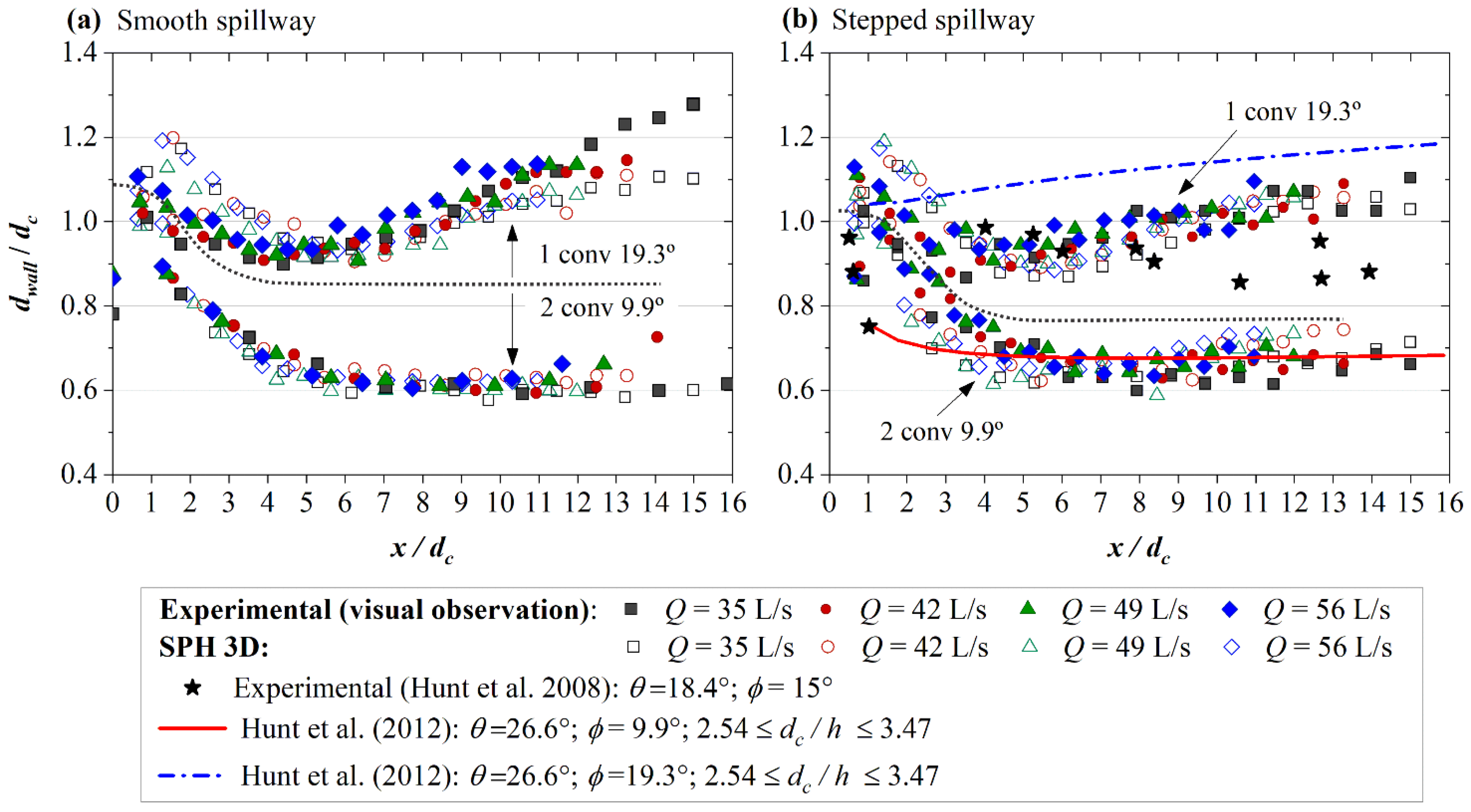
The flow depth development at the converging wall, normalized by the critical flow depth at the broad crested weir (, over the smooth spillway, is presented in Figure 7a. A marked effect of the wall convergence angle on is noticeable, with larger values being obtained for = 19.3°. On the other hand, the influence of the discharge on is relatively small. Overall, the general trends of the normalized flow depth profiles at the converging wall along the smooth spillway were reasonably well predicted by the 3D SPH simulations, particularly for = 9.9°.
The experimental and numerical results of over the smooth spillway with = 9.9° attained maximum values of approximately 1.0, near the upstream end of the chute, and stabilized around 0.6, downstream of 5. On the smooth spillway with = 19.3°, the flow depths decreased until 5 and continuously increased downstream of this location. The maximum values of for 19.3° varied approximately between 1.1 and 1.3.
The flow depth development of over the stepped spillway is presented in Figure 7b. Experimental data presented by [2], on a chute with an angle = 18.4° from the horizontal and a converging wall of = 15° (i.e., between = 9.9° and = 19.3°) are also plotted in Figure 7b, along with the results obtained from the relationship developed by [29], for converging stepped spillways, using = 26.6° and = 9.9° or = 19.3°. To obtain the curve from [29], the equations from [52] were first used to calculate (depending on , , and their relationship for the inception position), applicable to constant width chutes. Then, the equation developed by [29] for converging stepped spillways was used to calculate , and was finally obtained.
Similarly to the findings on smooth chutes, is significantly influenced by the wall convergence angle on the stepped chute, with larger values being obtained for = 19.3° (Figure 7b). On the other hand, the influence of the discharge on is relatively small. Overall, the general trends of the normalized flow depth profiles at the converging walls on the stepped spillway were reasonably well predicted by the 3D SPH simulations, particularly for = 9.9°, except on the upstream end of the chute.
The values of obtained on the stepped spillway with = 9.9° are consistent with the relationship of [29], but on the reach < 2.5. It should be noted that, in the latter study, the geometry of the crest as well as the relative location of start of converging wall were dissimilar from those adopted in the present study, which may explain the distinct trends of in the initial chute reach.
Considering the data for = 9.9° and the range of discharges, the maximum numerical value for was approximately 1.0 at the upstream end of the chute, stabilizing further downstream around 0.7. The maximum corresponding experimental values of varied between 0.94 and 1.0, which are of the same order of magnitude of the maximum value of = 0.92, predicted using the relationship from [7] for the same wall convergence angle. Nevertheless, it is important to highlight that the empirical relationship from [7] derived from experiments on a 1V:0.89H ( = 48.3°) sloping stepped spillway, with varying between 12° and 22.6°.
For the wall convergence angle of = 19.3° and the range of discharges, the maximum experimental value of was approximately 1.1, at the upstream or downstream ends of the chute (Figure 7b). This result is consistent with the maximum flow depth experimentally determined by [2], 1.0, for = 18.4° and = 15°, or the maximum value predicted using the relationship from [29], for = 26.6° and = 19.3°. However, they are smaller than the maximum value of = 1.39 obtained using the formulation from [7], which resulted from experimental measurements on a steeper stepped spillway. Although the maximum experimental or numerical values near the upstream or downstream ends of the chute are of the same order of magnitude as those found using the relationship from [29], the flow depth developments are different, probably as a result of the dissimilar geometry of the crest and distinct relative location of start of converging wall.
3.3. Velocity Profiles along the Spillway
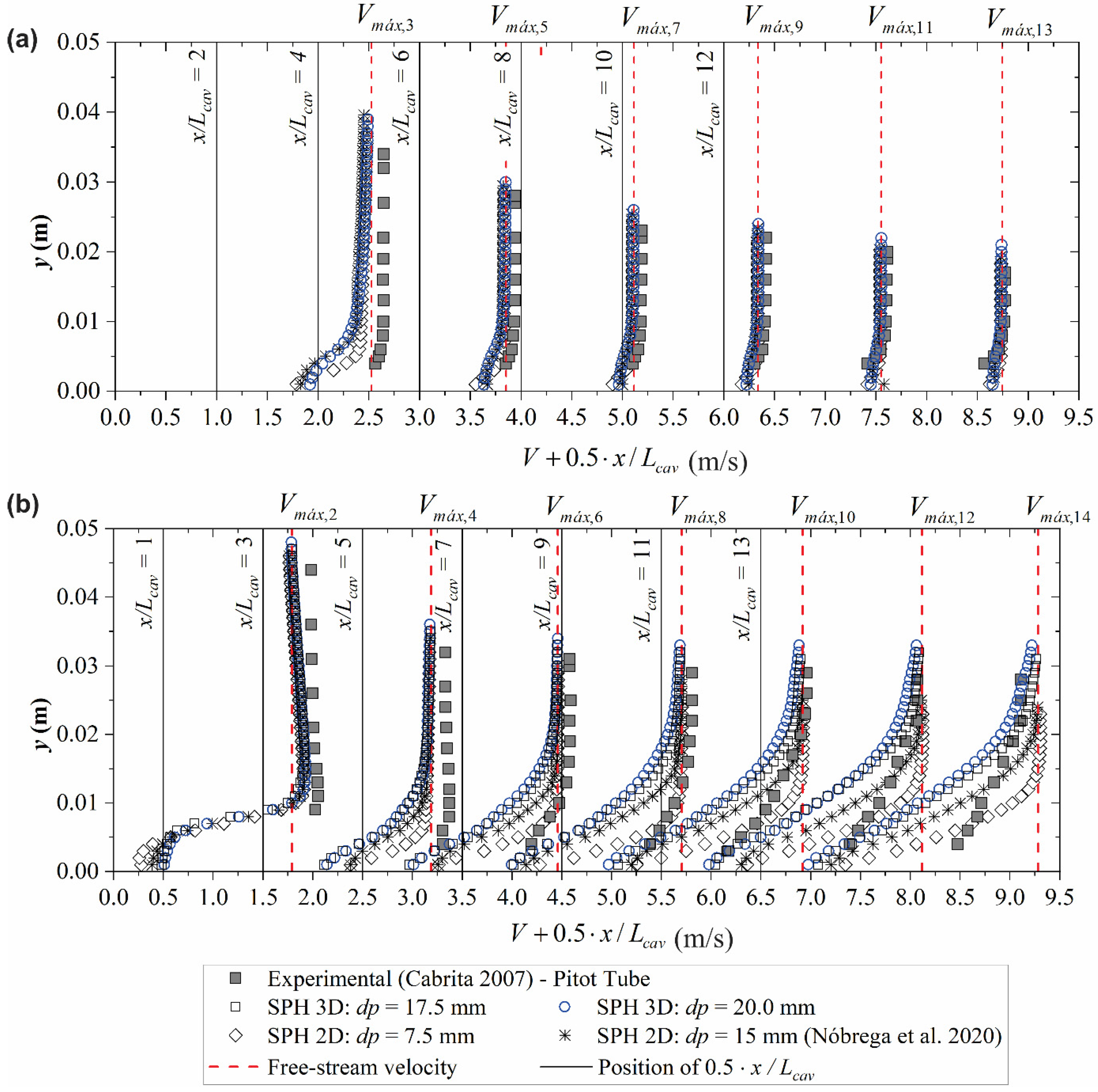
The experimental velocity profiles along the smooth and the stepped spillways with = 9.9° were analyzed and compared with the results from the 3D SPH simulations using = 20 mm and the 2D SPH simulations using = 7.5 and 15.0 mm from [34] (Figure 8).
To calculate the free-stream velocities, presented in Figure 8, the ideal-flow theory was used as , where is the gravity acceleration constant, is the upstream total head relative to the invert, is the flow depth measured at the flume centerline, and is the chute angle from the horizontal.
On the smooth spillway, the numerical velocity profiles from the 3D SPH model were similar to those obtained from the 2D SPH model using = 7.5 mm or 15.0 mm, presented by [34] (Figure 8a). The largest percentage differences between the experimental and the numerical velocity profiles on the smooth spillway were found at the positions = 2 and 4, because of the SPH particles’ detachment at the transition from the broad crested weir to the spillway. Inaccuracies on the experimental velocity measurements close to the upstream end of the chute are also expected, because of the hydrostatic pressure assumptions when calculating the velocities from the Prandtl–Pitot tube measurements. For the following cross sections ( > 4), the mean percentage differences for each cross section reduced with the longitudinal distance and were limited to 5% for the range of discharges.
On the stepped spillway, the free-stream velocities were well predicted by the 3D SPH simulations; however, the numerical results significantly underestimated the experimental counterparts near the invert (Figure 8b). The numerical velocity profiles were also comparable to the results obtained from the 3D or 2D SPH models using = 17.5 mm and = 15 mm (from [34]), respectively, with a slightly increasing deviation near the downstream end of the chute. Considering that numerical velocity profiles on the constant width stepped spillway were significantly dependent on , as shown by [34] for 2D SPH simulations, a better accuracy of the results near the pseudo-bottom would be expected by reducing the value of in the 3D SPH model. Similarly, as observed for the broad crested weir, the dynamic boundary conditions (DBCs) are also expected to influence the accuracy of the velocities near the solid boundary, because of the unphysical gap between the fluid particles and the fixed boundary, as mentioned by [40,49].
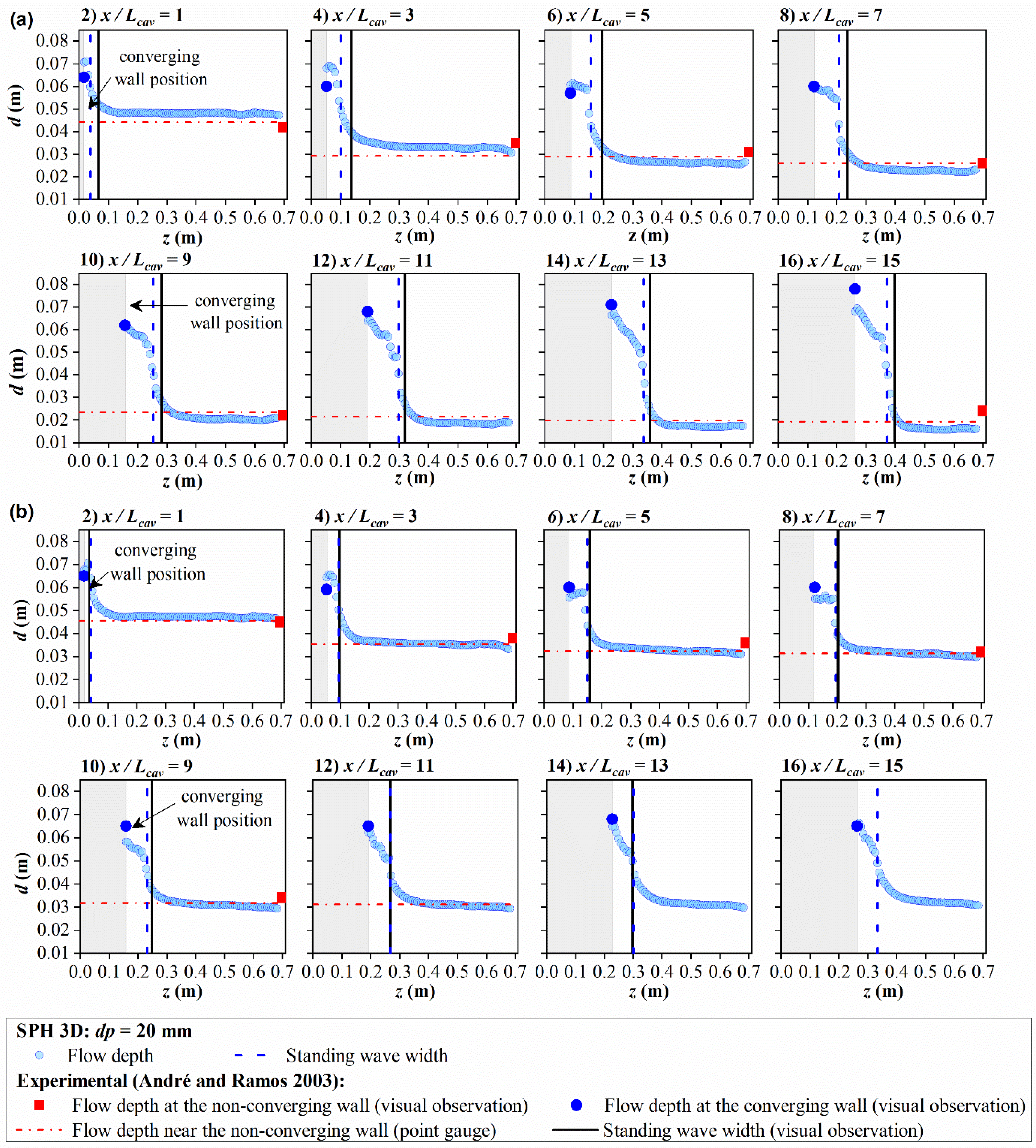
3.4. Cross-Sectional Flow Depth Profiles and Standing Wave Development along the Spillway
The numerical cross-sectional flow depth profiles are presented in Figure 9 and Figure 10 for = 9.9° and 19.3°, respectively. These figures include the following: (i) the experimental flow depths measured at the spillway centerline () or at the non-converging wall representing the pseudo-centerline (; (ii) the experimental flow depths at the converging wall (); (iii) the experimental standing wave widths, estimated visually or using the micro-propeller current meter; and (iv) the numerical standing wave widths, based on the criterion of the transverse position corresponding to the half-height of the standing wave (half value between and , for the spillway with two converging walls, or between and , for the spillway with one converging wall). In Figure 9 and Figure 10, the limit of the rectangles outlined in gray indicates the variable position of the converging wall.
Figure 9 and Figure 10 show that, near the upstream end of the chute, the flow depth is practically constant through the cross section, except in a short region close to the converging walls. This result agrees with the characteristic trapezoidal shape of the free surface in a cross section, as observed by [7]. The extension of the region influenced by the converging wall, with higher flow depths, increases in the downstream direction, as expected, owing to the increase in the standing wave width. The overall shape of the standing waves differs with the chute macro-roughness (i.e., smooth versus stepped inverts). In fact, both the height ( or ) and the width of the standing wave tend to be smaller in the stepped chute, as clearly visible on the downstream half of the chute (see Figure 9a versus Figure 9b and Figure 10a versus Figure 10b). Further, the general shape of the standing wave depends on the wall convergence angle. An increased wall convergence angle leads to a more abrupt flow depth change of the standing wave, and to an increase in the standing wave width, for an identical distance along the chute (see Figure 9a versus Figure 10a and Figure 9b versus Figure 10b).
In general, similar experimental and numerical flow depths were obtained at the centerline and wall of the spillway, except near the upstream or downstream ends of the chute. In addition, fairly comparable results of the standing wave width were in general obtained from experimental observations or numerical simulations. The experimental standing wave widths, either determined visually or using the micro-propeller current meter, corresponded approximately to transverse positions with sharped variations of the numerical flow depths.
From the numerical cross-sectional flow depth profiles of the stepped chute with = 9.9° (Figure 9b), a slight reduction in the flow depths for the smaller initial particle spacing used in simulations ( = 17.5 mm) is generally observed in comparison with the results obtained using = 20 mm. However, the flow depths near the converging wall were found to be practically independent of the tested values of .
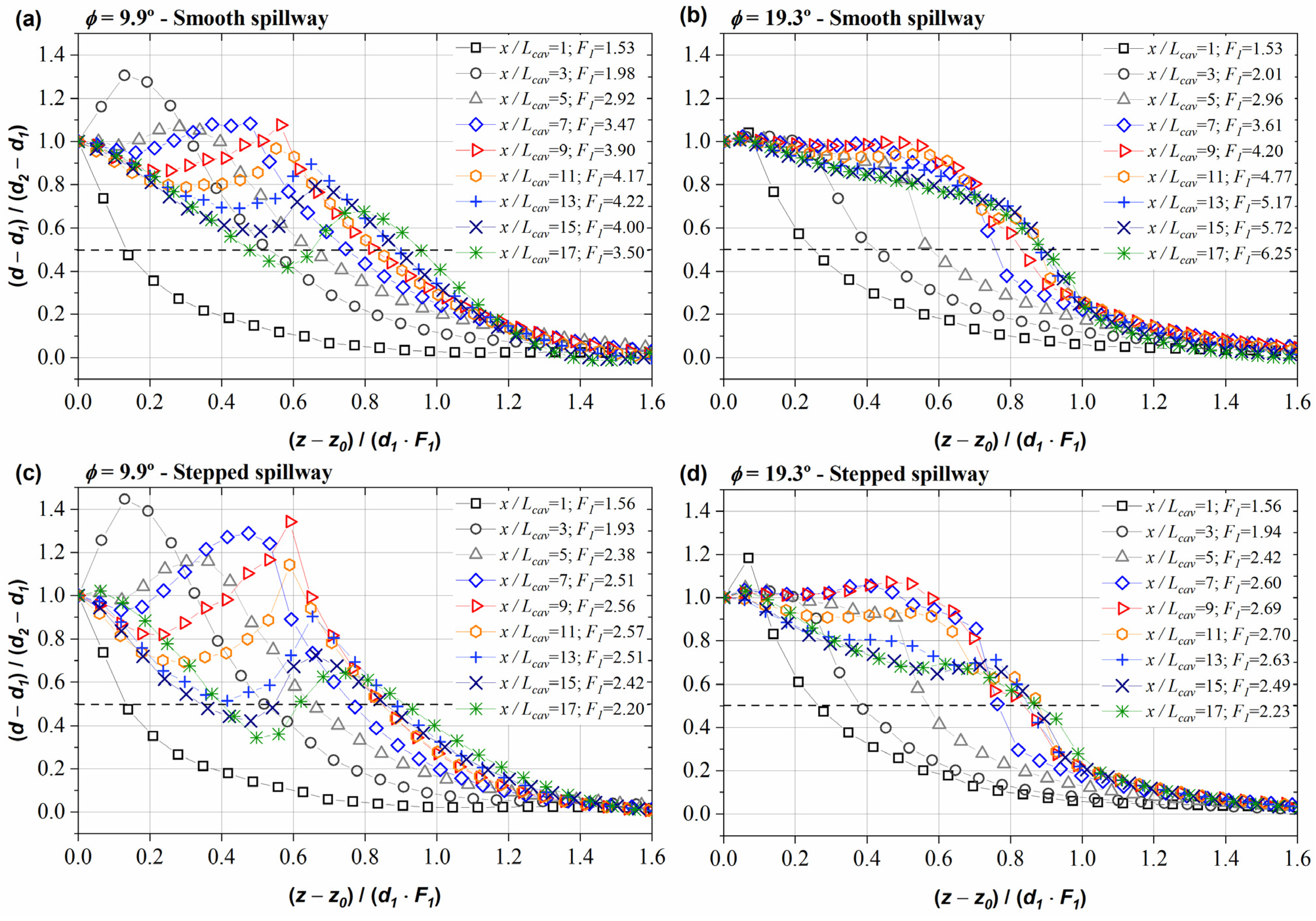
Normalized graphs for the standing wave are presented in Figure 11, for the discharge of 56 L/s. In this figure, is the flow depth; is the flow depth at the centerline () or at the non-converging wall (); is the flow depth at the converging wall (); is the transverse coordinate from the right wall of the broad crested weir; is the transverse coordinate from the right wall of the converging chute; is the local Froude number from the numerical results; is the streamwise coordinate; and is step cavity length, parallel to the pseudo-bottom (see Figure 1). The local Froude number was calculated as , where is the mean flow velocity given by the ratio between the approach unit flow rate and (), obtained from the numerical results. The dashed line given by = 0.5 represents the simplistic approximation used herein to define the standing wave front and its corresponding transverse position.
Figure 11 shows a considerable influence of the wall convergence angle on the general shape of the cross-sectional normalized flow depth profiles, except near the upstream end of the chute (i.e., ≤ 3) (see Figure 11a versus Figure 11b and Figure 11c versus Figure 11d). There, the cross-sectional flow depth profiles are markedly distinct from those found further downstream, as would be expected because of the inaccuracy of the present SPH simulations in this initial reach of the chute, as discussed in [34]. In contrast, the shape of the cross-sectional normalized flow depth profiles was not so markedly influenced by the chute macro-roughness (smooth or stepped inverts) (see Figure 11a versus Figure 11c and Figure 11b versus Figure 11d).
In general, the standing wave in the vicinity of the 9.9° converging wall was undular, for shock numbers () varying from 0.31 to 0.32, on the smooth and the stepped chutes (Figure 11). In the vicinity of the 19.3° converging wall, for = 0.60 to 0.63, the standing wave was similar to a roller type jump, presenting a constant or decreasing flow depth near the wall, followed by its abrupt change with the transverse coordinate. These observations are in conformity with the criterion proposed by [12] to classify the standing waves on horizontal channels, as undular standing waves if < 0.5 (presenting surface undulations comparable to an undular hydraulic jump), or over forced standing waves if > 1.8 to 2.0 (presenting excessively high wall waves, breaking of the shock front, and air entrainment). One can also notice that the simplistic approximation used herein to define the standing wave front is generally better suited for = 19.3°, because the wave fronts changed more abruptly than those found for = 9.9° (Figure 11).
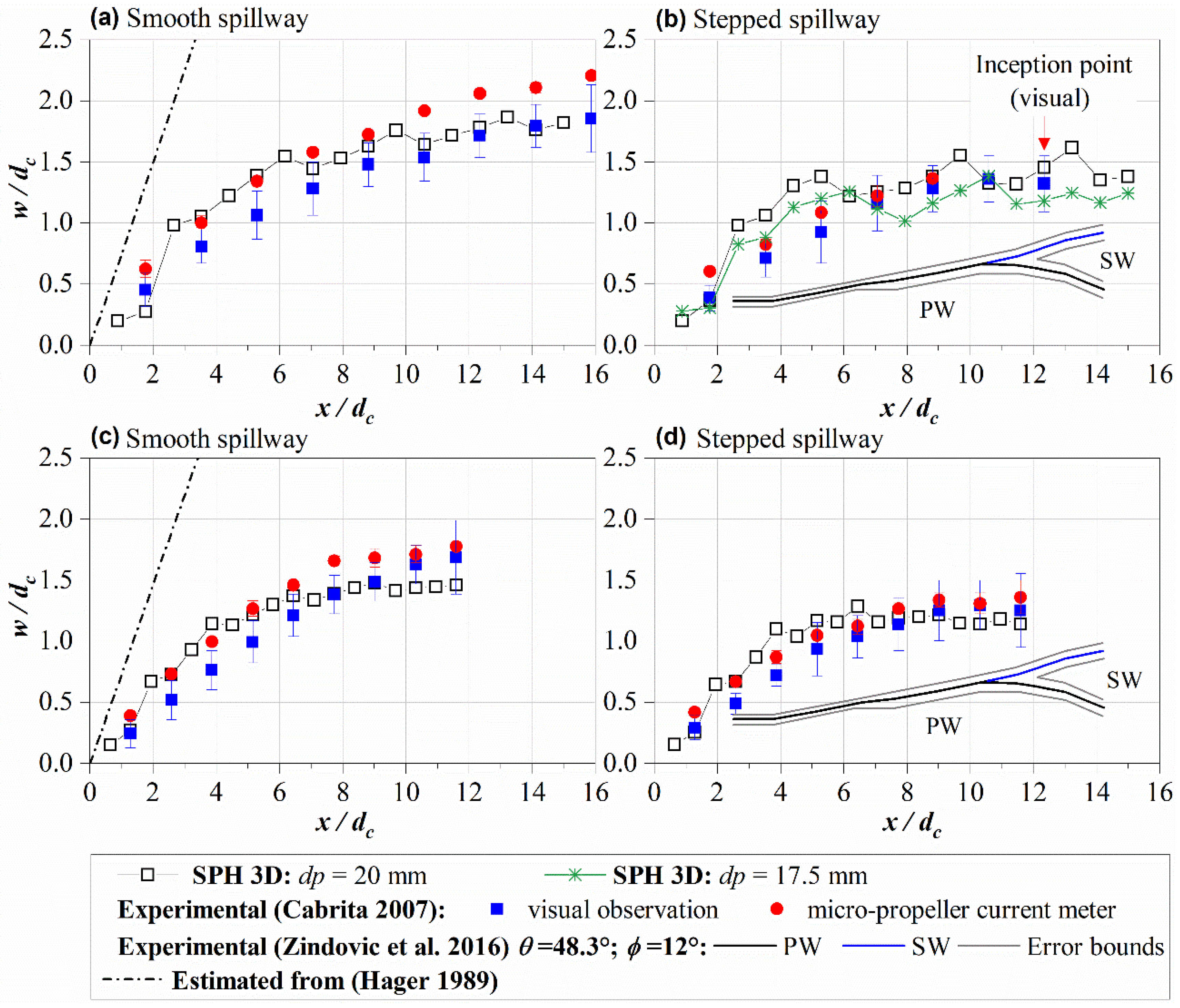
Typical developments of the standing wave width normalized by the critical flow depth at the broad crested weir () are shown in Figure 12 and Figure 13, for = 35 and 56 L/s, along the smooth and stepped spillways with two converging walls of = 9.9° or one converging wall of = 19.3°, respectively. The development of the normalized standing wave width () along the chute was found to be practically independent of the discharge, but markedly influenced by the chute macro-roughness. Near the downstream end of the chute, the normalized standing wave width () is considerably reduced on the stepped invert, for identical wall convergence angle and discharge (see Figure 12a versus Figure 12b and Figure 12c versus Figure 12d). In all test cases, one can observe an initial larger rate of increase in with distance and a milder increase further downstream, tending to nearly constant values, namely on the stepped chute. The boundary between these regions was found to occur for of approximately 6 to 8, regardless of the chute macro-roughness, discharge, and wall convergence angle. The standing wave width estimated from visual observations was in general smaller than that determined using the micro-propeller current meter, mainly on the smooth spillway. The results obtained by [7], on a 1V:0.89H ( = 48.3°) sloping stepped spillway (Figure 12b,d and Figure 13a,b), are significantly distinct from those obtained in this study, suggesting an effect of the chute slope on the development of the standing wave.
The influence of the chute macro-roughness on the standing wave width is evident from Figure 12 and Figure 13. For 10, 1.5–1.7 on the smooth chutes ( = 9.9° or = 19.3°). However, on the corresponding stepped chutes, for 10, 1.2–1.3, implying a reduction in the standing wave width of about 20 to 25%, in relation to that obtained on the smooth chute counterparts.
The dashed lines in Figure 12 and Figure 13 were obtained from the standing wave angle estimated from [54], at the origin of the chute contraction, as a function of the approach Froude number. The so-obtained angles are considerably larger than those estimated from the experimental data or numerical simulations near the chute origin, for = 9.9° (Figure 12a,b), but provide closer estimates for = 19.3° (Figure 13). This may be explained, in part, by the absence of experimental data in the upstream end of the chute, namely for = 9.9°.
Overall, the numerical standing wave widths were in relatively good agreement with the experimental data for = 9.9° (Figure 12), and the overall trend remained similar regardless of the initial particle spacing tested in the present study (i.e., = 20 and 17.5 mm). On the spillway with = 19.3° (Figure 13), reasonably good agreement was also obtained between the numerical and experimental data, except near the upstream end of the chute. It should be noted that, for this wall convergence angle, only data based on visual observation were collected.
3.5. Velocity and Vorticity Fields along the Stepped Spillway
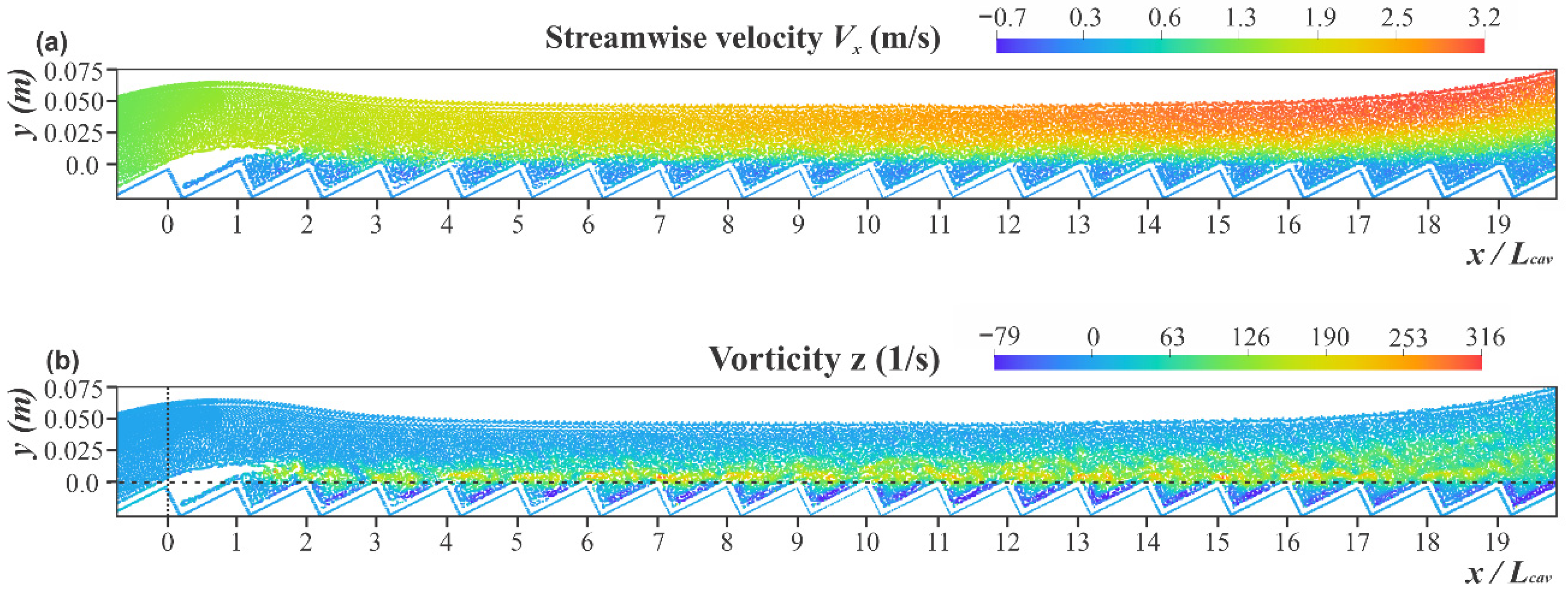
The instantaneous streamwise velocity () and spanwise vorticity () contour fields at the stepped spillway centerline with = 9.9° are shown in Figure 14a,b, respectively, for = 56 L/s. The streamwise velocity , parallel to the pseudo-bottom, tends to increase along the chute, from approximately 1.3 to 3.2 m/s. On the other hand, smaller values of the streamwise velocity, varying from −0.7 m/s to 0.3 m/s, were obtained within the step cavity, for = 56 L/s.
In the shear layer above the outer step edges, the largest value of the spanwise vorticity () was approximately 300 s−1 for = 56 L/s, near the pseudo-bottom. This result is fairly similar to the results from the 2D SPH simulations carried out by [34], for a similar setup and discharge. Values with the same order of magnitude were also obtained by [55,56] for an experimental setup with a steeper slope (51.3°) and = 2.15, using a particle image velocimetry (PIV) technique, as well to the numerical results presented by [57,58] for the mentioned experimental setup of [55,56]. Negative values of were found near the horizontal and vertical step faces (~−80 s−1), indicating counterclockwise vortices at these regions. Similar observations within the step cavities were obtained in [57], which presented maximum negative values for in the order of −150 s−1.
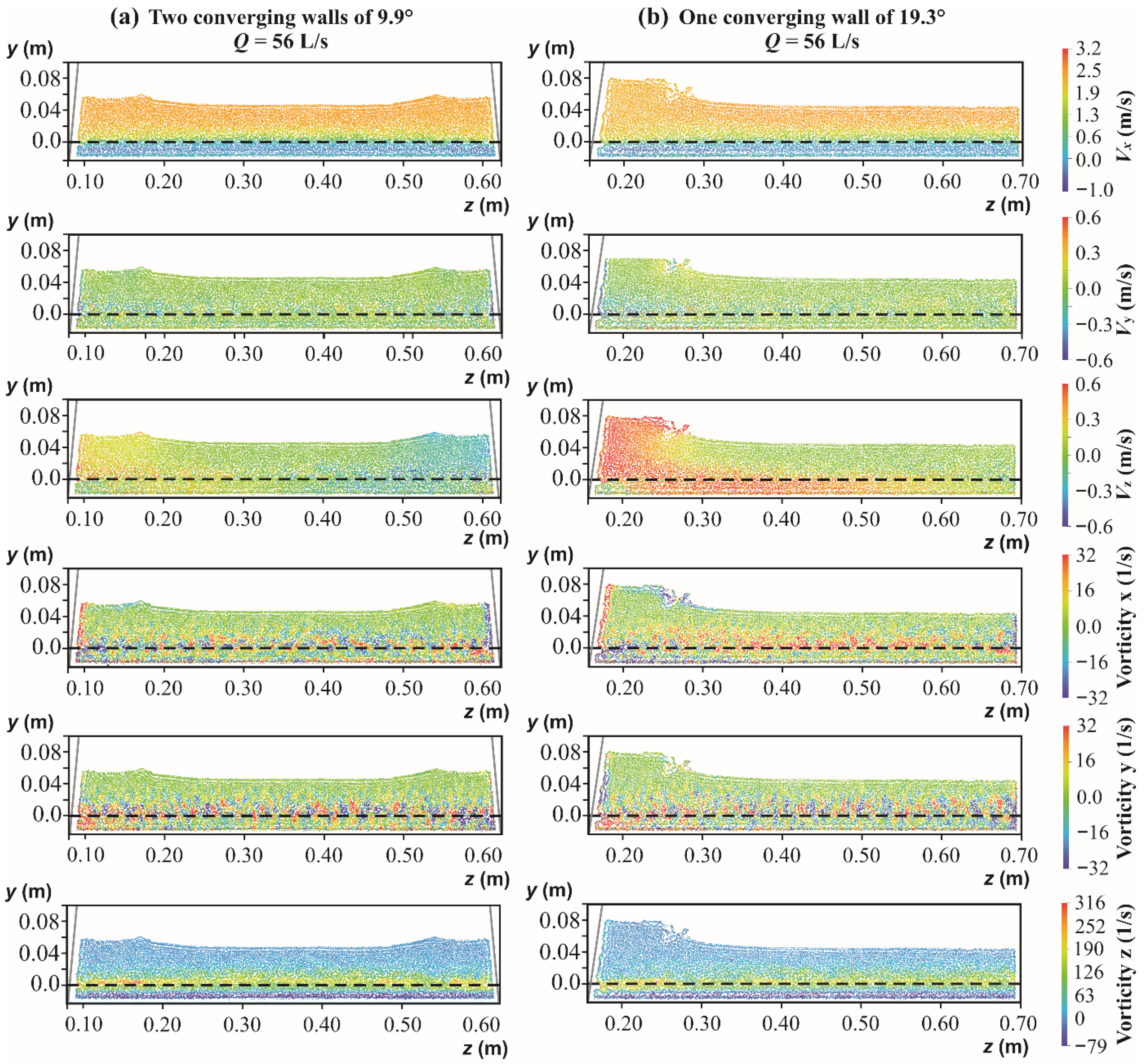
Instantaneous velocity and vorticity contour fields on a plane passing through the inner edge of the 10th step, perpendicular to the pseudo-bottom, for = 56 L/s are also shown in Figure 15. There, y and z are the normal from the pseudo-bottom and transverse coordinates, respectively. The dashed lines represent the pseudo-bottom and the oblique gray lines represent the intersection of the above referred plane with the converging wall. The spanwise velocity near the converging wall increased with the wall convergence angle, as would be expected. The maximum velocity was approximately 0.6 m/s for = 19.3° and 0.3 m/s for = 9.9°. The effect of the converging wall on near or below the pseudo-bottom seems to extend beyond the standing wave width, up to the transverse positions 0.35 for = 9.9°, and 0.5 for = 19.3°, as shown in Figure 15a,b. The effect of the converging wall on the streamwise and normal components of the velocity, and , respectively, was less evident in comparison with that on .
From the vorticity fields shown in Figure 15, namely those related to the streamwise and normal directions ( and ), the three-dimensionality of the recirculating vortices is identified, with positive and negative alternating values in the transverse direction, with maximum absolute values of approximately 30 s−1. The maximum values of the spanwise vorticity () were of the order of 300 s−1, similar to that presented in Figure 14, near the pseudo-bottom. Cavity recirculation vortices were also illustrated in experimental studies (e.g., [59]) and from numerical simulations based on mesh-based methods (e.g., [57,58,60]) for constant width spillways.
4. Conclusions
In supercritical flows, wall deflections lead to the formation of oblique standing waves, flow depth rise near the converging walls, and uneven distribution of the flow across the channel. The occurrence of standing waves on converging spillways was studied herein by means of three-dimensional numerical simulations using the SPH method. The spillway comprised a broad crested weir followed by a 1V:2H sloping spillway, typical on embankment dams, with smooth and stepped inverts, and wall convergence angles of 9.9° and 19.3°.
A marked effect of the wall convergence angle () on the flow depth development at the converging wall was noticeable. In fact, higher flow depths were observed at the converging wall, for larger . The flow depths at the chute centerline or the pseudo-centerline (for the spillway with one converging wall of 19.3°) were in general unaffected by the wall convergence, except near the downstream end of the chute, particularly on the stepped chute.
The chute macro-roughness was found to influence the height of the standing wave, leading to an attenuated effect for larger macro-roughness, that is, on the stepped chute. Moreover, the chute macro-roughness greatly influenced the typical development of the standing wave width along the chute, reducing the width on the stepped invert in comparison with that on the smooth invert.
The analysis of the numerical cross-sectional flow depth profiles showed that the general shape of the standing waves changes considerably with the wall convergence angle, yet it does not markedly change with the chute macro-roughness (smooth or stepped inverts). The numerical cross-sectional flow depth profiles presented an undular shape for the wall convergence angle of 9.9°, whereas a standing wave similar to a roller type jump was noted for the wall convergence angle of 19.3°. The dissimilar pattern of the standing wave was related to the approach shock number, which depends on the Froude number at the broad crested weir, immediately upstream of the wall deflection, and the wall convergence angle.
Overall, the numerical results agreed generally well with the experimental data on the broad crested weir and the spillway chute, namely, flow depths, velocity profiles, and the development of the standing wave width on the chute. The numerical results slightly overestimated the flow depths at the stepped chute centerline or pseudo-centerline, mainly near its downstream end. A reasonably good agreement was achieved for the flow depths at the converging walls, except on the upstream end of the chute, near the transition from the broad crested weir to the spillway. The numerical standing wave widths were also in relatively good agreement with the experimental counterparts. The velocity profiles along the broad crested weir and along the centerline of the 9.9° converging spillway also agreed generally well with the experimental data, near the free surface. The differences in the flow velocity were more significant close to the pseudo-bottom, particularly on the stepped chute. In order to overcome these limitations, simulations using the modified dynamic boundary conditions (mDBC), implemented in the current version of DualSPHysics, should be explored in further studies.
SPH velocity contour fields evidenced the effect of the converging wall on the spanwise velocity component, which increased with the wall convergence angle. SPH vorticity fields were comparable to those obtained experimentally or numerically from the literature, on constant width chutes. The three-dimensionality of the recirculating vortices in the step cavities was also identified from the vorticity field relative to the streamwise and normal directions.
Author Contributions
Conceptualization, J.D.N. and J.M.; Data curation, J.D.N. and J.M.; Formal analysis, J.D.N., J.M., H.E.S. and R.B.C.; Funding acquisition, J.M. and H.E.S.; Investigation, J.D.N. and J.M.; Methodology, J.D.N., J.M., H.E.S. and R.B.C.; Project administration, J.M.; Resources, J.M. and H.E.S.; Supervision, J.M. and H.E.S.; Visualization, J.D.N., J.M., H.E.S. and R.B.C.; Writing—original draft, J.D.N. and J.M.; Writing—review and editing, J.D.N., J.M., H.E.S. and R.B.C. All authors have read and agreed to the published version of the manuscript.
Funding
The Ph.D. scholarship granted to the first author, within the scope of the present study, was funded by the Coordination for the Improvement of Higher Education Personnel (CAPES)—(1413942), National Council for Scientific and Technological Development (CNPq)—(161809/2015-4; 140059/2018-0) in Brazil, and by Erasmus Mundus Project-Smart2 Scholarship (2014-0882/001-001).
Data Availability Statement
Some or all data that support the findings of this study are available from the corresponding author upon reasonable request.
Acknowledgments
The authors acknowledge the support of the Portuguese Foundation for Science and Technology (FCT), through the Project RECI/ECM-HID/0371/2012, and to Rui Ferreira in particular, for providing the computational server to run the simulations. Thanks also are extended to Luís Palma Mendes for his computational assistance.
Conflicts of Interest
The authors declare no conflict of interest.
Abbreviation
| speed of sound; | |
| numerical speed of sound; | |
| numerical density diffusion term; | |
| flow depth; | |
| initial particle spacing; | |
| critical flow depth at the broad crested weir; | |
| flow depth at the chute centerline; | |
| flow depth at the converging wall; | |
| flow depth at or near the non-converging wall; | |
| flow depth at the chute centerline immediately upstream of the wall deflection at = 0; | |
| flow depth at the chute centerline () or at the non-converging wall (); | |
| flow depth at the converging wall (); | |
| approach Froude number: ; | |
| local Froude number: ; | |
| continuous function; | |
| g | gravity acceleration constant; |
| g | gravity acceleration vector; |
| upstream total head relative to the invert; | |
| upstream total head above the broad crested weir; | |
| step height; | |
| kernel function length; | |
| length of the step cavity, parallel to the pseudo-bottom; | |
| length of the broad crested weir; | |
| step length; | |
| mass of the particle; | |
| pressure; | |
| discharge; | |
| unit discharge relative to the upstream width of the chute; | |
| normalized particle spacing in relation to the kernel function length: ; | |
| hydraulic radius; | |
| Reynolds number: ; | |
| r | position vector; |
| approach shock number: ; | |
| time; | |
| flow velocity; | |
| mean flow velocity at the chute centerline or at the non-converging wall: ; | |
| free-stream velocity; | |
| velocity vector; | |
| vorticity magnitude; | |
| smoothing kernel function; | |
| upstream width of the chute, at the downstream end of the broad crested weir; | |
| downstream width of the chute, at at the upstream end of the stilling basin; | |
| standing wave width; | |
| streamwise coordinate, parallel to the bottom or the pseudo-bottom; | |
| * | streamwise coordinate, parallel to the broad crested weir bottom; |
| normal coordinate, perpendicular to the bottom or the pseudo-bottom; | |
| * | normal coordinate, perpendicular to the broad crested weir bottom; |
| transverse coordinate, from the right wall of the broad crested weir; | |
| transverse coordinate from the right wall of the converging chute; | |
| coefficient of the Wendland kernel function; | |
| dissipation terms of the momentum equation; | |
| exponent of the equation of state; | |
| coefficient of the Delta-SPH function for the continuity equation; | |
| chute angle from the horizontal; | |
| kinematic viscosity; | |
| density of the particle; | |
| reference density; | |
| wall convergence angle; | |
| stress tensor. | |
| Subscripts | |
| interpolating particle; | |
| neighboring particle; | |
| values between particle and ; | |
| x | streamwise coordinate, parallel to the bottom or the pseudo-bottom; |
| normal coordinate, perpendicular to the bottom or the pseudo-bottom; | |
| transverse coordinate, from the right wall of the broad crested weir. | |
References
- USBR. Spillways. In Design of Small Dams, 3rd ed.; United States Department of the Interior: Washington, DC, USA, 1987; pp. 339–434. [Google Scholar]
- Hunt, S.L.; Kadavy, K.C.; Abt, S.R.; Temple, D.M. Impact of converging chute walls for roller compacted concrete stepped spillways. J. Hydraul. Eng. 2008, 134, 1000–1003. [Google Scholar] [CrossRef]
- Moran, R.; Toledo, M.A.; Peraita, J.; Pellegrino, R. Energy dissipation in stilling basins with side jets from highly convergent chutes. Water 2021, 13, 1343. [Google Scholar] [CrossRef]
- Dawson, J.H. The Effect of Lateral Contractions on Super-Critical Flow in Open Channels. M.Sc. Thesis, Lehigh University, Bethlehem, PA, USA, 1943. [Google Scholar]
- Ippen, A.T.; Dawson, J.H. Design of channel contractions. T. Am. Soc. Civ. Eng. 1951, 116, 326–346. [Google Scholar] [CrossRef]
- Hager, W.H.; Schwalt, M.; Jimenez, O.; Chaudhry, M.H. Supercritical flow near an abrupt wall deflection. J. Hydraul. Res. 1994, 32, 103–118. [Google Scholar] [CrossRef]
- Zindovic, B.; Vojt, P.; Kapor, R.; Savic, L. Converging stepped spillway flow. J. Hydraul. Res. 2016, 54, 699–707. [Google Scholar] [CrossRef]
- Stone, A.A. Theoretical Investigation of Standing Waves in Hydraulic Structures. M.Sc. Thesis, Massachusetts Institute of Technology, Cambridge, MA, USA, 1946. [Google Scholar]
- Ippen, A.T.; Harleman, D.R.F. Verification of theory for oblique standing waves. T. Am. Soc. Civ. Eng. 1956, 121, 678–694. [Google Scholar] [CrossRef]
- Nikpour, M.R.; Khosraviniab, P.; Farsadizadehc, D. Experimental analysis of shock waves turbulence in contractions with rectangular sections. J. Comp. Appl. Res. Mech. Eng. 2018, 8, 189–198. [Google Scholar] [CrossRef]
- Reinauer, R.; Hager, W.H. Shockwave reduction by chute diffractor. Exp. Fluids 1996, 21, 209–217. [Google Scholar] [CrossRef]
- Reinauer, R.; Hager, W.H. Supercritical flow in chute contraction. J. Hydraul. Eng. 1998, 124, 55–64. [Google Scholar] [CrossRef]
- Jiménez, O.F. Computation of Supercritical Flow in Open Channels. M.Sc. Thesis, Washington State University, Pullman, WA, USA, 1987. [Google Scholar]
- Jiménez, O.F.; Chaudhry, M.H. Computation of supercritical free-surface flows. J. Hydraul. Eng. 1988, 114, 377–395. [Google Scholar] [CrossRef]
- Causon, D.M.; Minghan, C.G.; Ingram, D.M. Advances in calculation methods for supercritical flow in spillway channels. J. Hydraul. Eng. 1999, 125, 1039–1050. [Google Scholar] [CrossRef]
- Abdo, K.; Riahi-Nezhad, K.C.; Imran, J. Steady supercritical flow in a straight-wall open-channel contraction. J. Hydraul. Res. 2018, 57, 647–661. [Google Scholar] [CrossRef]
- Neilson, F.M. Convex Chutes in Converging Supercritical Flow; Report; U.S. Army Engineer Waterways Experimentation Station Hydraulics Laboratory: Vicksburg, MS, USA, 1976. [Google Scholar]
- Jan, C.-D.; Chang, C.-J.; Lai, J.-S.; Guo, W.-D. Characteristics of hydraulic shock waves in an inclined chute contraction—Experiments. J. Mech. 2009, 25, 129–136. [Google Scholar] [CrossRef]
- Frizell, K.H. Hydraulic Model Study of Mc Clure Dam Existing and Proposed RCC Stepped Spillways; Report n. R-90-02; U.S. Department of the Interior, Bureau of Reclamation: Denver, CO, USA, 1990. [Google Scholar]
- Hanna, L.J.; Pugh, C.A. Hydraulic Model Study of Pilar Dam; Report, U.S.; Department of the Interior, Bureau of Reclamation, Technical Service Center: Denver, CO, USA, 1997. [Google Scholar]
- André, M.; Ramos, P. Hidráulica de Descarregadores de Cheia em Degraus: Aplicação a Descarregadores com Paredes Convergentes; Research Report; Instituto Superior Técnico, Universidade de Lisboa: Lisbon, Portugal, 2003. [Google Scholar]
- Frizell, K.H. Hydraulic Model Study of Gwinnett County Georgia Y15 Dam Overtopping Protection; Report HL-20006-05; U.S. Department of the Interior, Bureau of Reclamation: Washington, DC, USA, 2006. [Google Scholar]
- Cabrita, J. Caracterização do Escoamento Deslizante Sobre Turbilhões em Descarregadores de Cheias em Degraus com Paredes Convergentes. M.Sc. Thesis, Instituto Superior Técnico, Universidade de Lisboa, Lisbon, Portugal, 2007. [Google Scholar]
- Hunt, S.L. Design of Converging Stepped Spillways. Ph.D. Thesis, Colorado State University, Fort Collins, CO, USA, 2008. [Google Scholar]
- Woolbright, R.W. Hydraulic Performance Evaluation of RCC Stepped Spillways with Sloped Converging Training Walls. Ph.D. Thesis, Oklahoma State University, Stillwater, OK, USA, 2008. [Google Scholar]
- Woolbright, R.W.; Hunt, S.L.; Hanson, G.J. Model study of RCC stepped spillways with sloped converging stepped spillway training walls. In Proceedings of the American Society of Agricultural and Biological Engineers, Providence, RI, USA, 29 June–2 July 2008. [Google Scholar] [CrossRef]
- Willey, J.; Ewing, T.; Lesleighter, E.; Dymke, J. Numerical and physical modelling for a complex stepped spillway. Hydropower Dams 2010, 17, 103–113. [Google Scholar]
- Wadhai, P.J.; Ghare, A.D.; Deshpande, N.V.; Vasudeo, A.D. Comparative analysis for estimation of the height of training wall of convergent stepped spillway. Int. J. Eng. Technol. 2015, 4, 294–303. [Google Scholar] [CrossRef] [Green Version]
- Hunt, S.L.; Temple, D.M.; Abt, S.R.; Kadavy, K.C.; Hanson, G. Converging stepped spillways: Simplified momentum analysis approach. J. Hydraul. Eng. 2012, 138, 796–802. [Google Scholar] [CrossRef]
- Reisi, A.; Salah, P.; Kavianpour, M.R. Impact of chute walls convergence angle on flow characteristics of spillways using numerical modeling. Int. J. Chem. Environ. Biol. Sci. 2015, 3, 245–251. [Google Scholar]
- Nunes, A.F.P. Modelação Computacional do Escoamento Deslizante Sobre Turbilhões em Descarregadores de Cheias em Degraus com Paredes Convergentes. M.Sc. Thesis, Instituto Superior Técnico, Universidade de Lisboa, Lisbon, Portugal, 2017. [Google Scholar]
- Nunes, F.; Matos, J.; Meireles, I. Numerical modelling of skimming flow over small converging spillways. In Proceedings of the 3rd International Conference on Protection against Overtopping, Protections 2018, Grange-over-Sands, UK, 6–8 June 2018. [Google Scholar]
- Salazar, F.; San-Mauro, J.; Celigueta, M.A.; Oñate, E. Shockwaves in spillways with the particle finite element method. Comput. Part. Mech. 2020, 7, 87–99. [Google Scholar] [CrossRef]
- Nóbrega, J.D.; Matos, J.; Schulz, H.E.; Canelas, R.B. Smooth and stepped spillway modelling using the SPH method. J. Hydraul. Eng. 2020, 146, 04020054. [Google Scholar] [CrossRef]
- López, D.; de Blas, M.; Marivela, R.; Rebollo, J.J.; Díaz, R.; Sánchez Juny, M.; Strella, S. Estudio hidrodinámico de vertederos y rápidas escalonadas con modelo numérico tridimensional SPH: Proyecto ALIVESCA. In Proceedings of the II Jornadas de Ingeniería del Agua: Modelos Numéricos en Dinámica Fluvial: FLUMEN, Barcelona, Spain, 5–6 October 2011. [Google Scholar]
- Gu, S.; Ren, L.; Wang, X.; Xie, H.; Huang, Y.; Wei, J.; Shao, S. SPHysics simulation of experimental spillway hydraulics. Water 2017, 9, 973. [Google Scholar] [CrossRef] [Green Version]
- Novak, P.; Moffat, A.I.B.; Nalluri, C.; Narayanan, R. Hydraulic Structures, 4th ed.; Taylor & Francis: New York, NY, USA, 2007. [Google Scholar]
- Liu, G.R.; Liu, M.B. Smoothed Particle Hydrodynamics: A Meshfree Particle Method, 1st ed.; World Scientific Publishing: Singapore, 2003. [Google Scholar]
- Crespo, A.J.C.; Domínguez, J.M.; Rogers, B.D.; Gómez-Gesteira, M.; Longshaw, S.; Canelas, R.; Vacondio, R.; Barreiro, A.; García-Feal, O. DualSPHysics: Open-source parallel CFD solver based on Smoothed Particle Hydrodynamics (SPH). Comput. Phys. Comm. 2015, 187, 204–216. [Google Scholar] [CrossRef]
- Domínguez, J.M.; Fourtakas, G.; Altomare, C.; Canelas, R.B.; Tafuni, A.; García-Feal, O.; Martínez-Estévez, I.; Mokos, A.; Vacondio, R.; Crespo, A.J.C.; et al. DualSPHysics: From fluid dynamics to multiphysics problems. Comput. Part. Mech. 2021, 9, 867–895. [Google Scholar] [CrossRef]
- Wendland, H. Piecewise polynomial, positive definite and compactly supported radial functions of minimal degree. Adv. Comput. Math. 1995, 4, 389–396. [Google Scholar] [CrossRef]
- Molteni, D.; Colagrossi, A. A simple procedure to improve the pressure evaluation in hydrodynamic context using the SPH. Comput. Phys. Commun. 2009, 180, 861–872. [Google Scholar] [CrossRef]
- Gotoh, H.; Shao, S.; Memita, T. SPH-LES model for numerical investigation of wave interaction with partially immersed breakwater. Coastal Eng. J. 2004, 46, 39–63. [Google Scholar] [CrossRef]
- Husain, S.M.; Muhammed, J.R.; Karunarathna, H.U.; Reeve, D.E. Investigation of pressure variations over stepped spillways using smooth particle hydrodynamics. Adv. Water Resour. 2014, 66, 52–69. [Google Scholar] [CrossRef]
- Wan, H.; Li, R.; Gualtieri, C.; Yang, H.; Feng, J. Numerical simulation of hydrodynamics and reaeration over a stepped spillway by the SPH method. Water 2017, 9, 565. [Google Scholar] [CrossRef] [Green Version]
- Wan, H.; Li, R.; Pu, X.; Zhang, H.; Feng, J. Numerical simulation for the air entrainment of aerated flow with an improved multiphase SPH model. Int. J. Comput. Fluid Dyn. 2017, 31, 435–449. [Google Scholar] [CrossRef]
- Felder, S.; Chanson, H. Free-surface profiles, velocity and pressure distributions on a broad-crested weir: A physical study. J. Irrig. Drain. Eng. 2012, 138, 1068–1074. [Google Scholar] [CrossRef] [Green Version]
- Lúcio, I. Modelação Numérica do Escoamento Deslizante Sobre Turbilhões em Descarregadores de Cheias em Degraus: Aplicação a Pequenas Barragens de Aterro. M.Sc. Thesis, Instituto Superior Técnico, Universidade de Lisboa, Lisbon, Portugal, 2015. [Google Scholar]
- English, A.; Domínguez, J.M.; Vacondio, R.; Crespo, A.J.C.; Stansby, P.K.; Lind, S.J.; Chiapponi, L.; Gómez-Gesteira, M. Modifed dynamic boundary conditions (mDBC) for general-purpose smoothed particle hydrodynamics (SPH): Application to tank sloshing, dam break and fish pass problems. Comp. Part. Mech. 2021, 9, 1–15. [Google Scholar] [CrossRef]
- Castro-Orgaz, O.; Hager, W.H. Drawdown curve and turbulent boundary layer development for chute flow. J. Hydraul. Res. 2010, 48, 591–602. [Google Scholar] [CrossRef]
- Nóbrega, J.D.; Matos, J.; Schulz, H.E.; Canelas, R.B. SPH simulation of non-aerated flow over converging spillways. In Proceedings of the 9th International Symposium on Hydraulic Structures: IAHR, IIT, Roorkee, India, 24–27 October 2022. accepted. [Google Scholar]
- Hunt, S.L.; Kadavy, K.C.; Hanson, G.J. Simplistic design methods for moderate-sloped stepped chutes. J. Hydraul. Eng. 2014, 40, 04014062. [Google Scholar] [CrossRef]
- Meireles, I.; Matos, J. Skimming flow in the nonaerated region of stepped spillways over embankment dams. J. Hydraul. Eng. 2009, 135, 685–689. [Google Scholar] [CrossRef]
- Hager, W.H. Supercritical flow in channel junctions. J. Hydraul. Eng. 1989, 115, 595–616. [Google Scholar] [CrossRef]
- Amador, A.T. Comportamiento Hidráulico de los Aliviaderos Escalonados en Presas de Hormigón Compactado. Ph.D. Thesis, Universitat Politècnica de Catalunya, Barcelona, Spain, 2005. [Google Scholar]
- Amador, A.; Sánchez-Juny, M.; Dolz, J. Characterization of the nonaerated flow region in a stepped spillway by PIV. J. Fluids Eng. Trans. ASME 2006, 128, 1266–1273. [Google Scholar] [CrossRef] [Green Version]
- Toro, J.P.; Bombardelli, F.A.; Paik, J. Detached eddy simulation of the nonaerated skimming flow over a stepped spillway. J. Hydraul. Eng. 2017, 143, 04017032. [Google Scholar] [CrossRef]
- Zabatela, F.; Bombardelli, F.A.; Toro, J.P. Towards an understanding of the mechanisms leading to air entrainment in the skimming flow over stepped spillways. Environ. Fluid Mech. 2020, 20, 375–392. [Google Scholar] [CrossRef]
- Matos, J.; Meireles, I. Hydraulics of stepped weirs and dam spillways: Engineering challenges, labyrinths of research. In Proceedings of the 5th IAHR International Symposium on Hydraulic Structures, Brisbane, Australia, 25–27 June 2014. [Google Scholar]
- Lopes, P.; Leandro, J.; Carvalho, R.F.; Bung, D.B. Alternating skimming flow over a stepped spillway. Environ. Fluid Mech. 2016, 17, 303–322. [Google Scholar] [CrossRef]
Figure 1.
Scheme of the physical model: (a) side view; (b) top view of the spillway with two converging walls of 9.9°; (c) top view of the spillway with one converging wall of 19.3°.
Figure 1.
Scheme of the physical model: (a) side view; (b) top view of the spillway with two converging walls of 9.9°; (c) top view of the spillway with one converging wall of 19.3°.

Figure 2.
Scheme of the computational domain and the initial numerical condition of the spillway with two converging walls of 9.9°. Schematic detail of the inlet open boundary adapted from [40].
Figure 2.
Scheme of the computational domain and the initial numerical condition of the spillway with two converging walls of 9.9°. Schematic detail of the inlet open boundary adapted from [40].

Figure 3.
(a) Flow depths over the broad crested weir for = 35 L/s ( = 0.063 m); (b) experimental versus numerical flow depths over the broad crested weir for = 35 to 56 L/s (0.063 ≤ (m) ≤ 0.087). References: Cabrita (2007) [23]; Lúcio (2015) [48]; Nunes (2017) [31]; Nóbrega et al. (2020) [34].

Figure 4.
Normalized velocity profiles along the broad crested weir for = 35 L/s ( = 0.063 m). References: Cabrita (2007) [23]; Lúcio (2015) [48]; Nóbrega et al. (2020) [34].

Figure 5.
Flow depths along the spillway: (a) smooth invert with two converging walls of = 9.9° and = 35 L/s ( = 0.063 m); (b) stepped invert with two converging walls of = 9.9° and = 35 L/s ( = 2.52); (c) smooth invert with one converging wall of = 19.3° and = 56 L/s ( = 0.087 m; (d) stepped invert with one converging wall of = 19.3° and = 56 L/s ( = 3.48). References: André and Ramos (2003) [21]; Cabrita (2007) [23]; Castro-Orgaz and Hager (2010) [50]; Hunt et al. (2014) [52]; Meireles and Matos (2009) [53]; Nóbrega et al. (2020) [34].

Figure 6.
Experimental versus numerical flow depths. Data at the centerline or near the non-converging wall (point gauge): (a) smooth spillway (0.063 ≤ (m) ≤ 0.087); (b) stepped spillway (2.52 ≤ ≤ 3.48). Data at the converging wall: (c) smooth spillway (0.063 ≤ (m) ≤ 0.087); (d) stepped spillway (2.52 ≤ ≤ 3.48) (experimental data from [23] for = 9.9° and from [21] for = 19.3°).

Figure 7.
Normalized flow depths at the converging wall (0.063 ≤ (m) ≤ 0.087): (a) smooth spillway; (b) stepped spillway (2.52 ≤ ≤ 3.48). (Data of [2] obtained through digitalization). References: Hunt et al. (2008) [2]; Hunt et al. (2012) [29].

Figure 8.
Velocity profiles along the spillway with two converging walls of = 9.9° for = 35 L/s ( = 0.063 m): (a) smooth spillway; (b) stepped spillway ( = 2.52). References: Cabrita (2007) [23]; Nóbrega et al. (2020) [34].

Figure 9.
Cross-sectional flow depth profiles for the spillway with two converging walls of = 9.9°, = 35 L/s ( = 0.063 m): (a) smooth spillway; (b) stepped spillway ( = 2.52). Reference: Cabrita (2007) [23].
Figure 9.
Cross-sectional flow depth profiles for the spillway with two converging walls of = 9.9°, = 35 L/s ( = 0.063 m): (a) smooth spillway; (b) stepped spillway ( = 2.52). Reference: Cabrita (2007) [23].

Figure 10.
Cross-sectional flow depth profiles for the spillway with one converging wall of = 19.3°, = 35 L/s ( = 0.063 m): (a) smooth spillway; (b) stepped spillway ( = 2.52). Reference: André and Ramos (2003) [21].
Figure 10.
Cross-sectional flow depth profiles for the spillway with one converging wall of = 19.3°, = 35 L/s ( = 0.063 m): (a) smooth spillway; (b) stepped spillway ( = 2.52). Reference: André and Ramos (2003) [21].

Figure 11.
Normalized cross-sectional flow depth profiles for = 56 L/s ( = 0.087 m): (a) smooth spillway, = 9.9°; (b) smooth spillway, = 19.3°; (c) stepped spillway, = 9.9° ( = 3.48); (d) stepped spillway, = 19.3° ( = 3.48).
Figure 11.
Normalized cross-sectional flow depth profiles for = 56 L/s ( = 0.087 m): (a) smooth spillway, = 9.9°; (b) smooth spillway, = 19.3°; (c) stepped spillway, = 9.9° ( = 3.48); (d) stepped spillway, = 19.3° ( = 3.48).

Figure 12.
Normalized standing wave width for the spillway with two converging walls of = 9.9°: (a) smooth spillway, = 35 L/s ( = 0.063 m); (b) stepped spillway, = 35 L/s ( = 2.52); (c) smooth spillway, = 56 L/s ( = 0.087 m); (d) stepped spillway, = 56 L/s ( = 3.48) (data of [7] obtained through digitalization: outer edge of the primary part (PW) of the standing wave and outer edge of the secondary part (SW) of the standing wave, along with error bounds for their small step model for = 3.36). References: Hager (1989) [54]; Cabrita (2007) [23]; Zindovic et al. (2016) [7].

Figure 13.
Normalized standing wave width for the smooth and stepped spillways with one converging wall of = 19.3°: (a) = 35 L/s ( = 0.063 m, = 2.52); (b) = 56 L/s ( = 0.087 m, = 3.48) (data of [7] obtained through digitalization: outer edge of the primary part (PW) of the standing wave and outer edge of the secondary part (SW) of the standing wave, along with error bounds for their small step model for = 3.36). References: Hager (1989) [54]; André and Ramos (2003) [21]; Zindovic et al. (2016) [7].

Figure 14.
Instantaneous contour fields at the chute centerline of the stepped spillway with two converging walls of 9.9°, for = 56 L/s ( = 0.087 m, = 3.48): (a) streamwise velocity ; (b) spanwise vorticity .
Figure 14.
Instantaneous contour fields at the chute centerline of the stepped spillway with two converging walls of 9.9°, for = 56 L/s ( = 0.087 m, = 3.48): (a) streamwise velocity ; (b) spanwise vorticity .

Figure 15.
Instantaneous velocity and vorticity contour fields on a plane passing through the inner edge of the 10th step, perpendicular to the pseudo-bottom, for = 56 L/s ( = 0.087 m, = 3.48) (the oblique gray line included in the graphs results from the intersection of this plane with the converging wall).


Table 1.
Summary of experimental studies on stepped spillways with converging walls.
| Reference | (°) | (°) | Measurements | |
|---|---|---|---|---|
| Frizell (1990) [19] | 24.6 | 0; 5.6; 12.7 | 0.76 to 8.82 | Spillway discharge capacity, flow depths, energy dissipation |
| Hanna and Pugh (1997) [20] | 51.3 | 16 | 1.54 to 4.50 | Flow depth profiles, pressure, energy dissipation |
| André and Ramos (2003) [21] | 26.6 | 0; 19.3 | 0.69 to 3.48 | Flow depths, standing wave width, angle of the standing wave front, velocities, energy dissipation |
| Frizell (2006) a [22] | 18.4 | 18.4 | 1.21 to 7.03 | Discharge capacity, flow dephts, velocities, flow run out |
| Cabrita (2007) [23] | 26.6 | 9.9; 19.3 | 0.90 to 3.48 | Flow depths, standing wave width and angle, velocities, energy dissipation |
| Hunt (2008) [24]; Hunt et al. (2008) [2] | 18.4 | 0; 15; 30; 52 | 1.83 to 6.04 | Flow depth profiles, standing wave width |
| Woolbright (2008) a [25]; Woolbright et al. (2008) a [26]; | 18.4 | 18; 34; 45 | 3.86 to 6.07 | Stepped and smoothed sloped converging training wall. Flow depths, run-up height, angle of the standing wave front |
| Willey et al. (2010) a [27] | 53.1 | 12 | 1.56 to 5.14 | Discharge capacity, flow depths and energy dissipation |
| Wadhai et al. (2015) [28] | 45.0 | 45 | 0.15 to 2.60 | Flow depths |
| Zindovic et al. (2016) [7] | 48.3 | 12; 18.8; 22.6 | 3.36 | Flow depths, standing wave width, air concentration, velocity profiles, residual energy |
a Stepped spillway with sloped converging training wall; is the chute angle from the horizontal; is the wall convergence angle; is the critical flow depth upstream of the channel contraction; is the step height.
Publisher’s Note: MDPI stays neutral with regard to jurisdictional claims in published maps and institutional affiliations. |
© 2022 by the authors. Licensee MDPI, Basel, Switzerland. This article is an open access article distributed under the terms and conditions of the Creative Commons Attribution (CC BY) license (https://creativecommons.org/licenses/by/4.0/).
Share and Cite
MDPI and ACS Style
Nóbrega, J.D.; Matos, J.; Schulz, H.E.; Canelas, R.B. Smooth and Stepped Converging Spillway Modeling Using the SPH Method. Water 2022, 14, 3103. https://doi.org/10.3390/w14193103
AMA Style
Nóbrega JD, Matos J, Schulz HE, Canelas RB. Smooth and Stepped Converging Spillway Modeling Using the SPH Method. Water. 2022; 14(19):3103. https://doi.org/10.3390/w14193103
Chicago/Turabian StyleNóbrega, Juliana D., Jorge Matos, Harry E. Schulz, and Ricardo B. Canelas. 2022. "Smooth and Stepped Converging Spillway Modeling Using the SPH Method" Water 14, no. 19: 3103. https://doi.org/10.3390/w14193103
Note that from the first issue of 2016, this journal uses article numbers instead of page numbers. See further details here.