
Prediction of the Amount of Sediment Deposition in Tarbela Reservoir Using Machine Learning Approaches
 ,
,  ,
,  ,
,  and
and 
Abstract
:1. Introduction
2. Literature Review
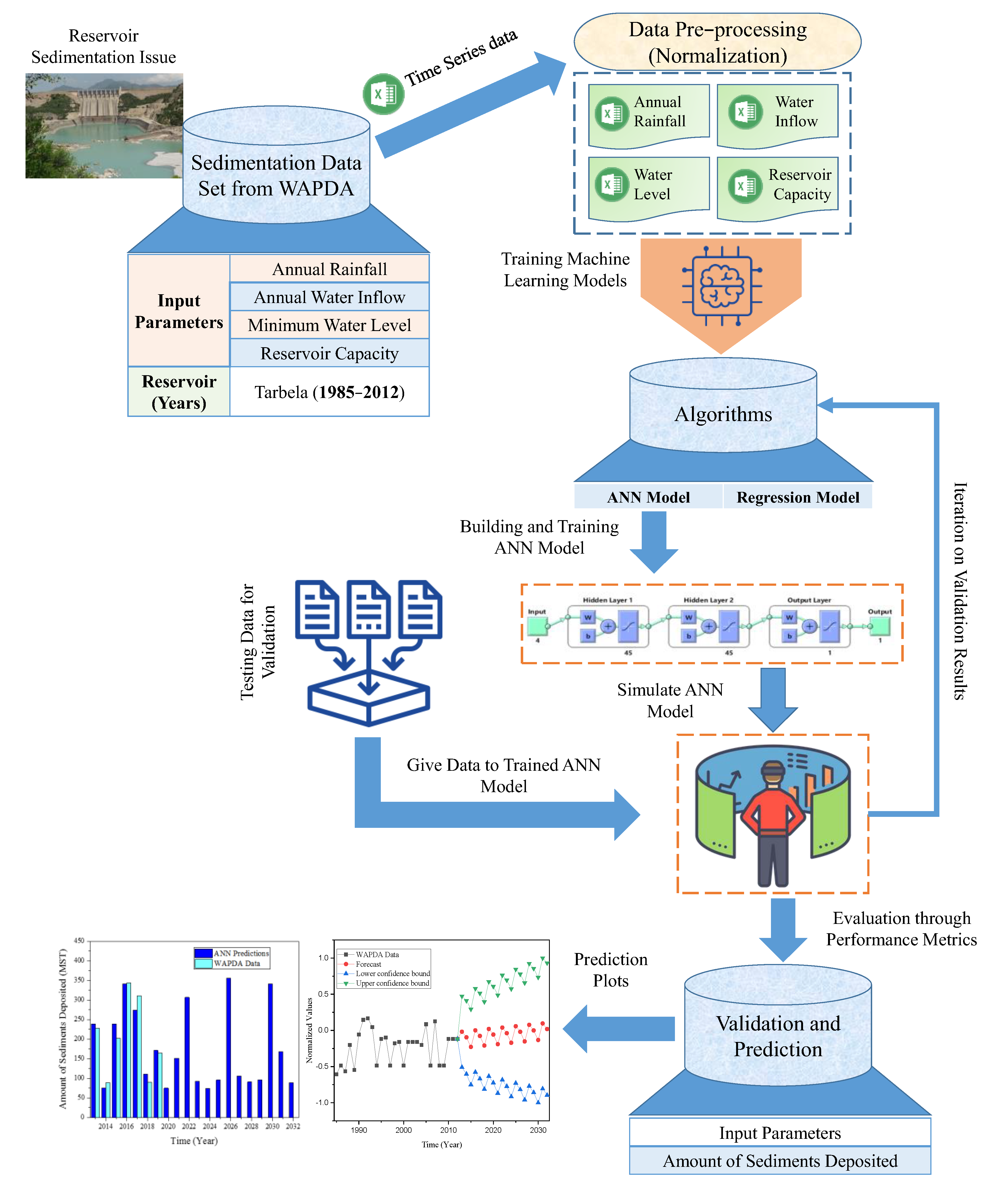
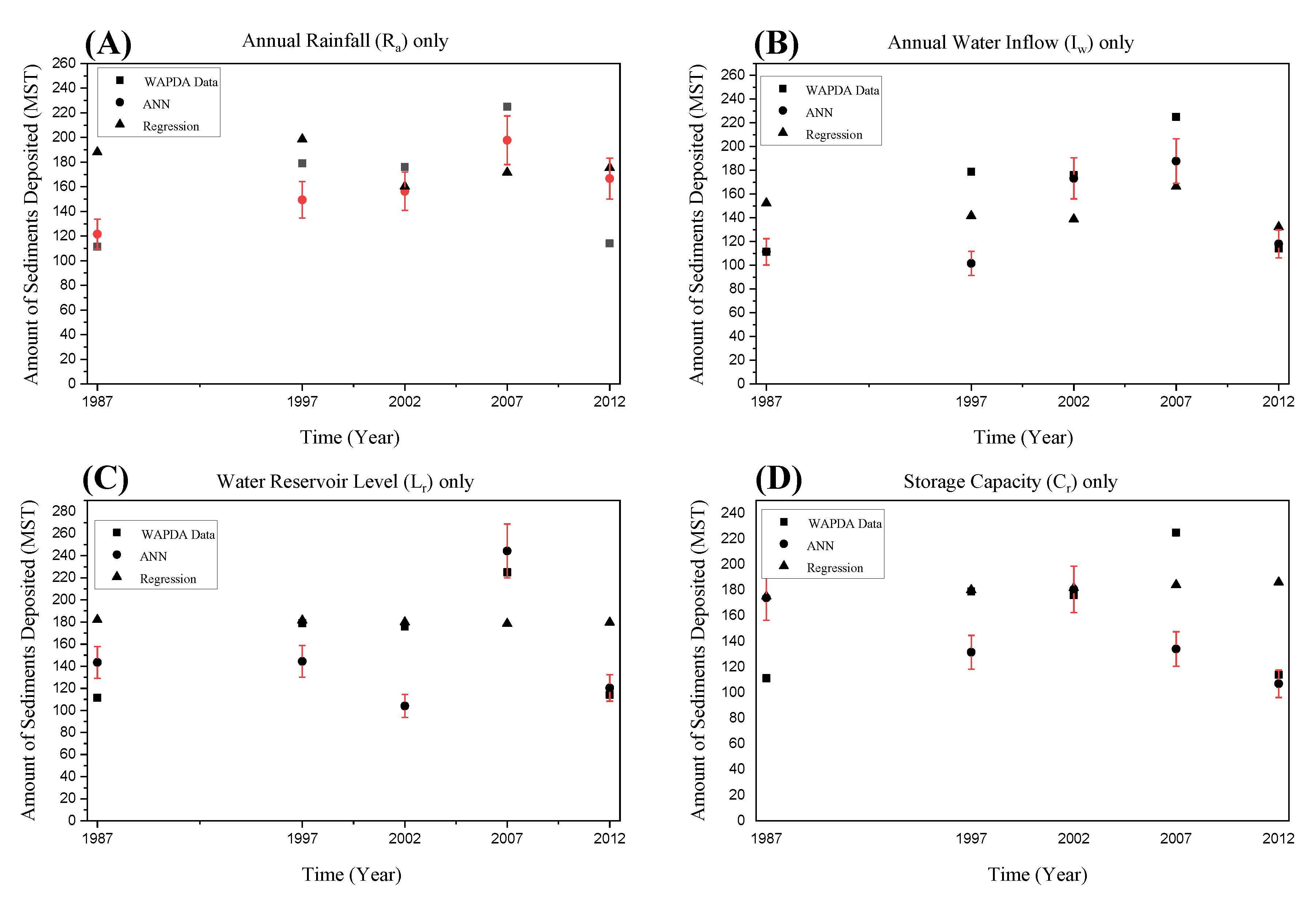
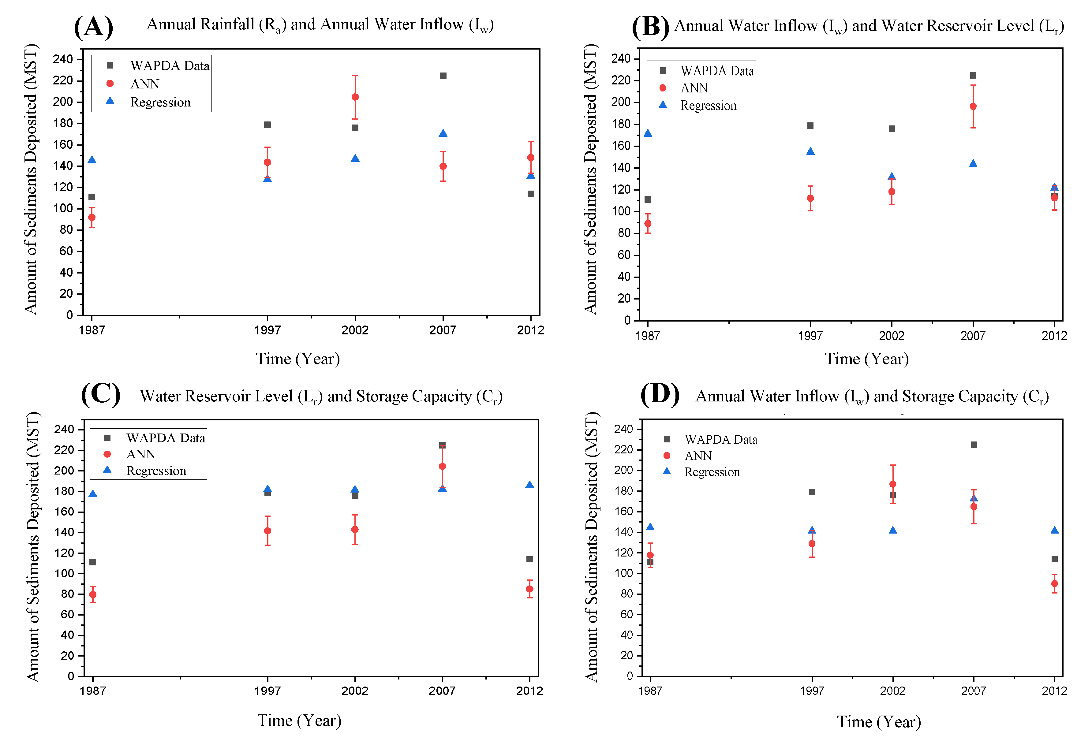
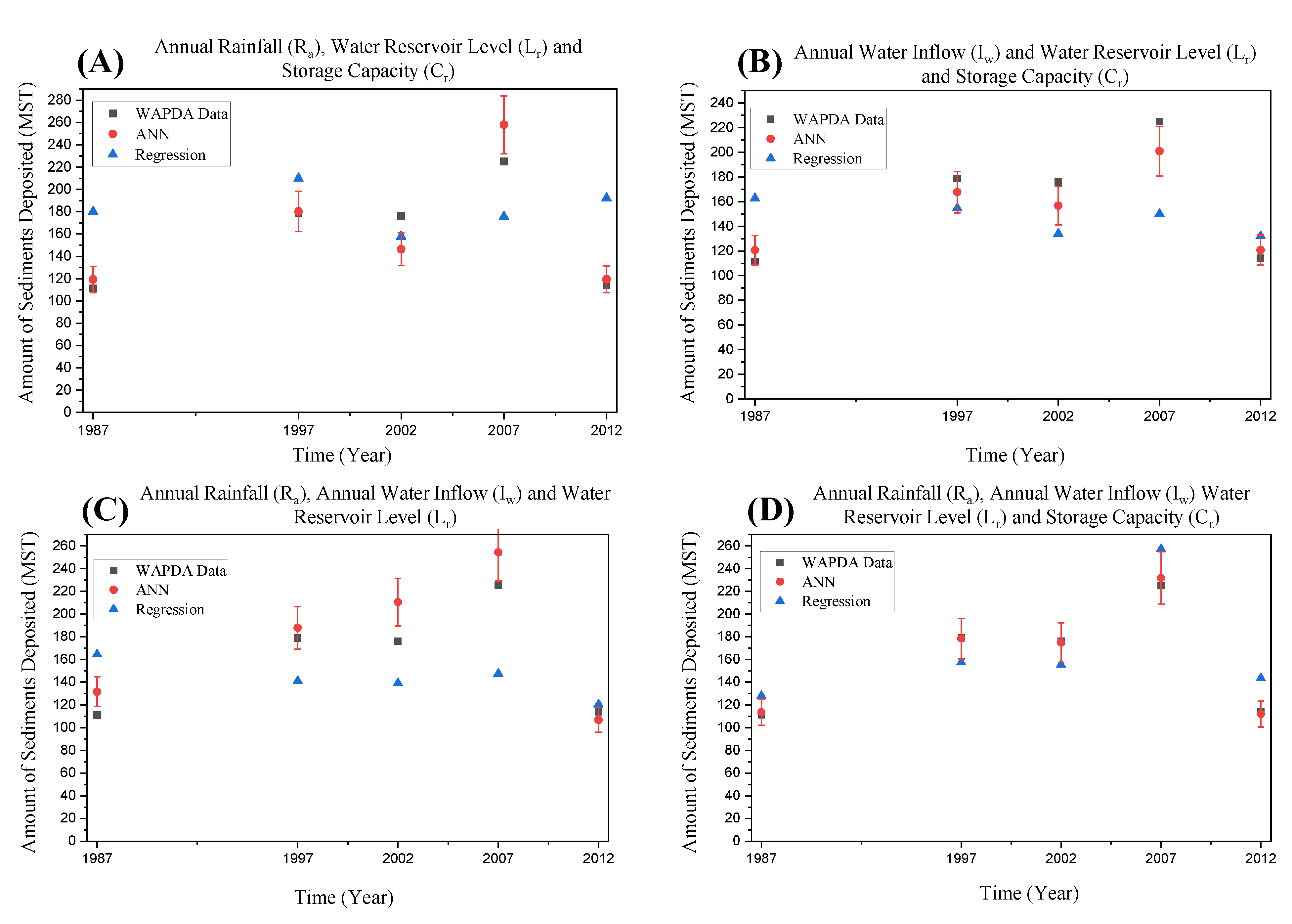
- To find the amount of sediment deposited inside the Tarbela reservoir using the proposed artificial neural network model and the multivariate regression model considering four yearly influencing factors: Ra, Iw, Lr, and Cr.
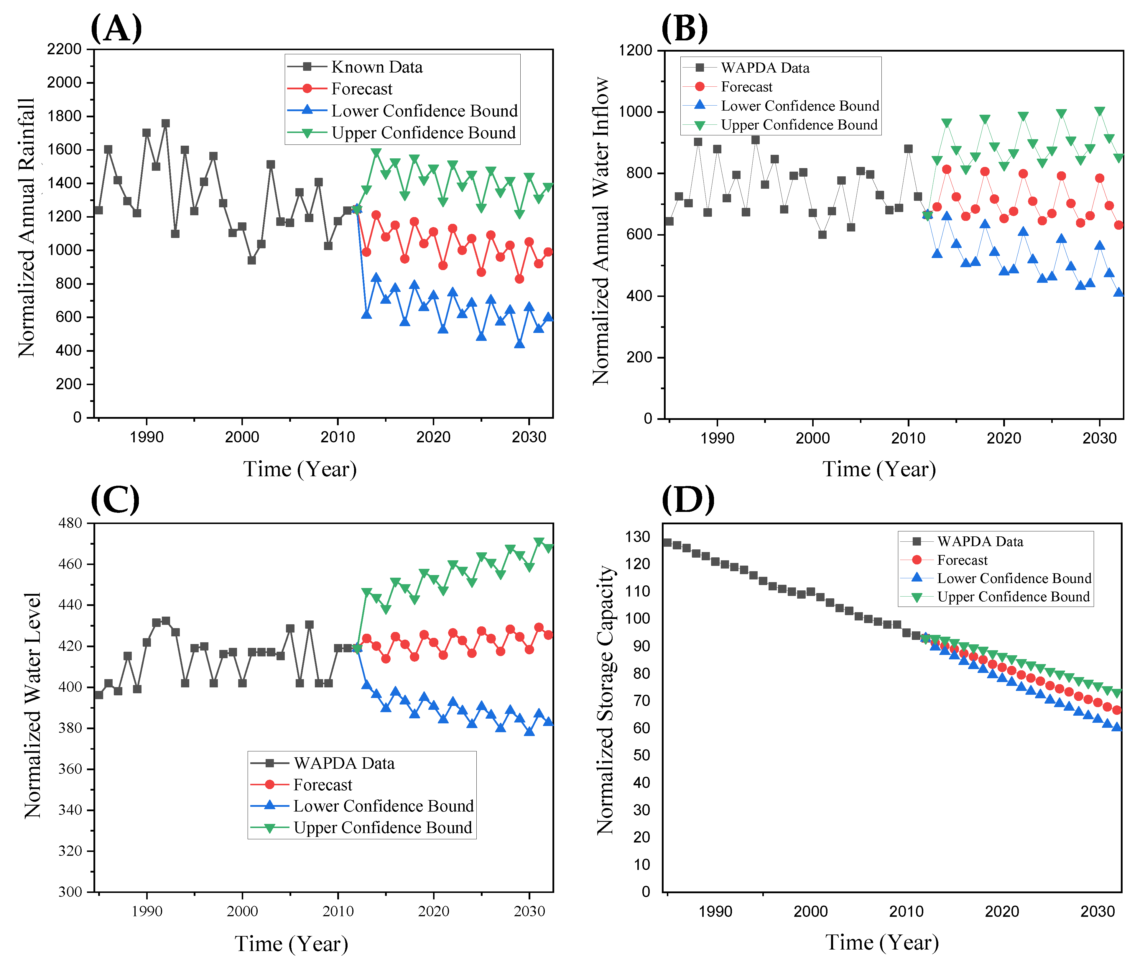
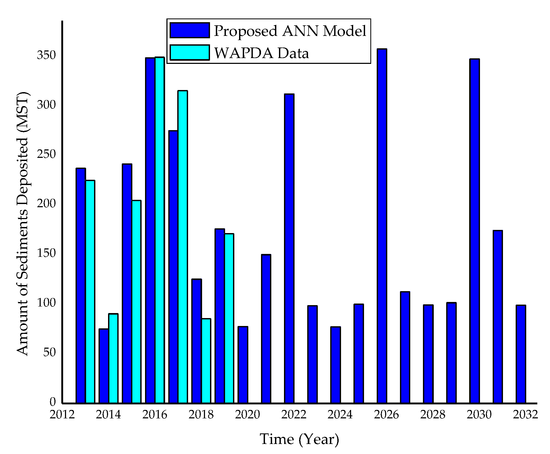
- To make future predictions of the sedimentation volume inside the Tarbela reservoir using trained ANN based on the time series univariate forecasting model ETS forecasted values of Ra, Iw, Lr, and Cr.
3. Materials and Methods
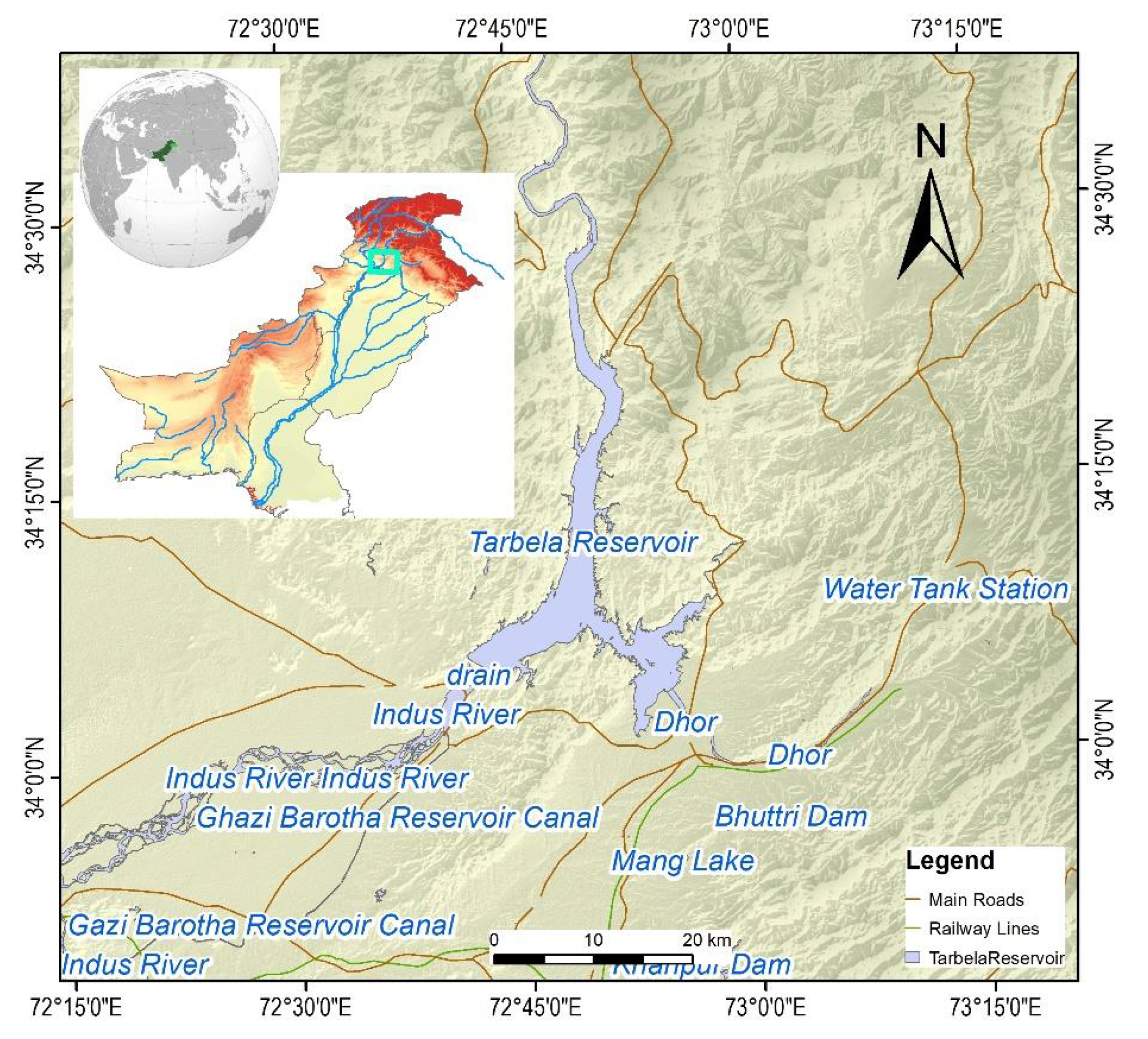
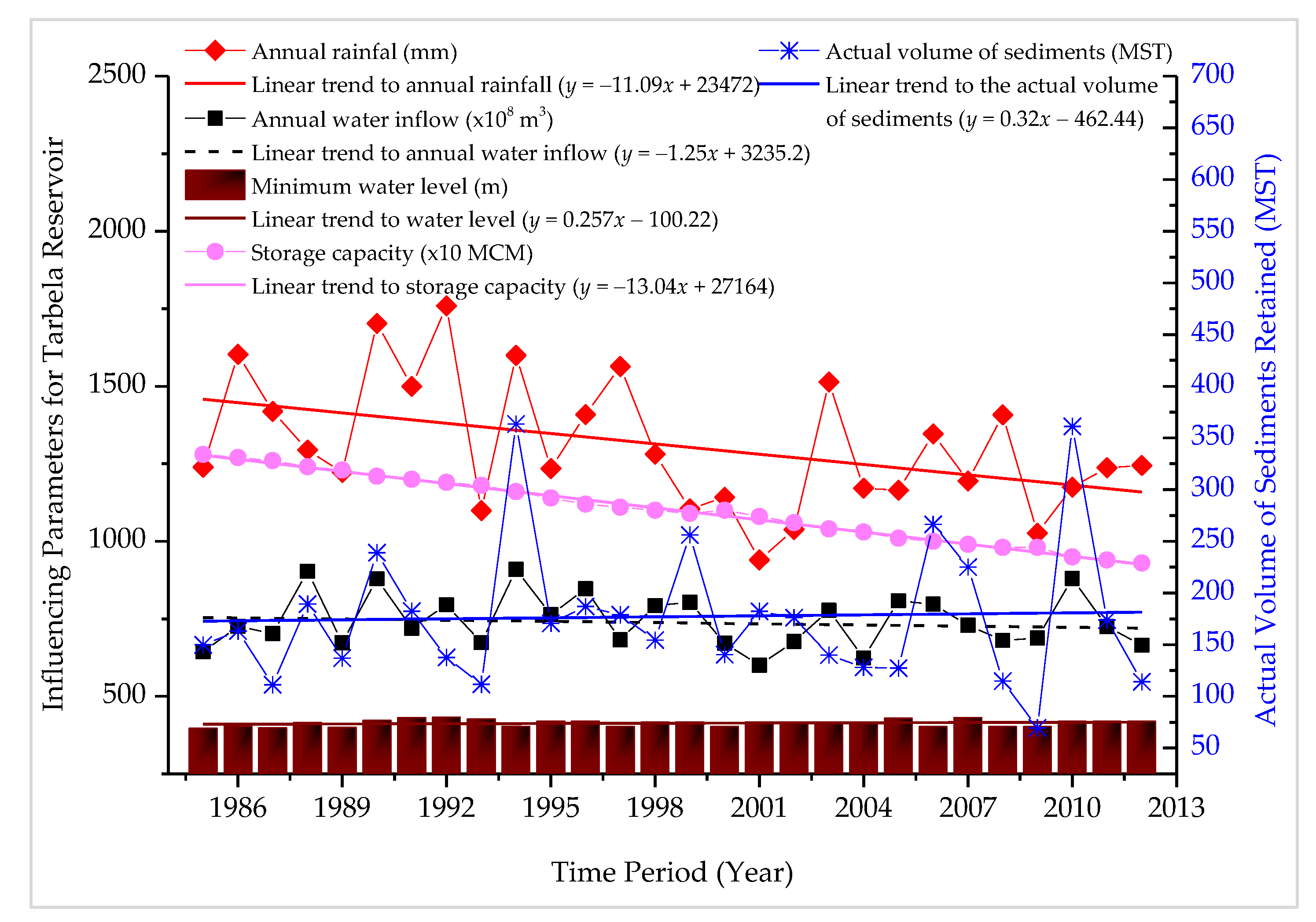
3.1. Study Areas and Data Collection
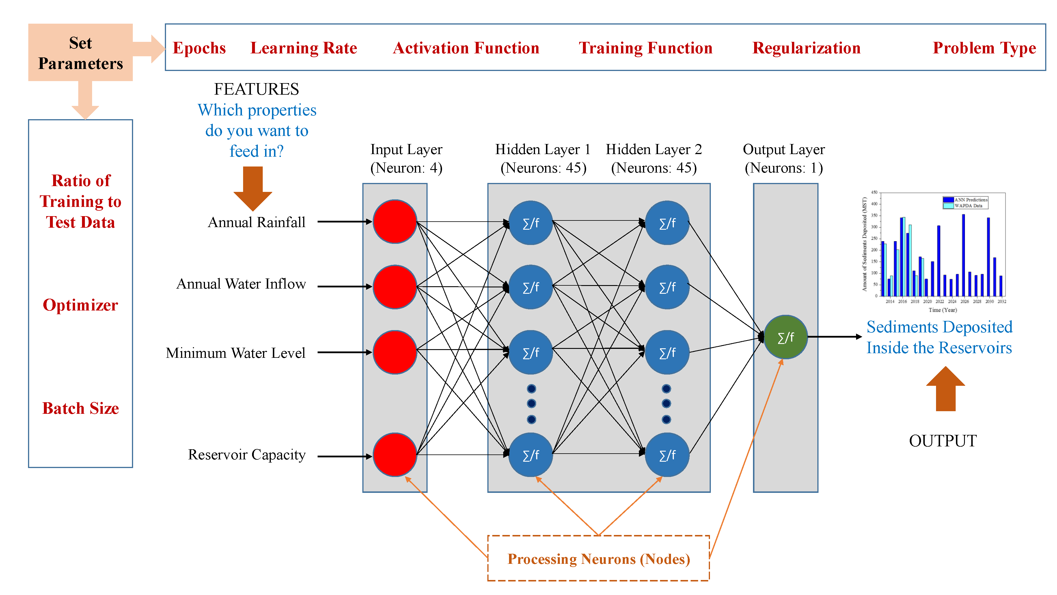
3.2. Model Development
3.3. Experimental Protocols and Performance Evaluation Measures
4. Results and Discussion
5. Conclusions
Author Contributions
Funding
Data Availability Statement
Acknowledgments
Conflicts of Interest
Nomenclature
| ANN | Artificial Neural Network |
| ETS | Error, Trend, Seasonal |
| MT | Million Tonnes |
| MST | Million Short Tons |
| MSE | Mean Squared Error |
| MAE | Mean Absolute Error |
| NSE | Nash–Sutcliffe Efficiency |
| Ra | Annual rainfall |
| Iw | Water inflow annually |
| LR | The minimum water level in the reservoir |
| Cr | Capacity of reservoir |
| SR | Amount of sediment deposited annually |
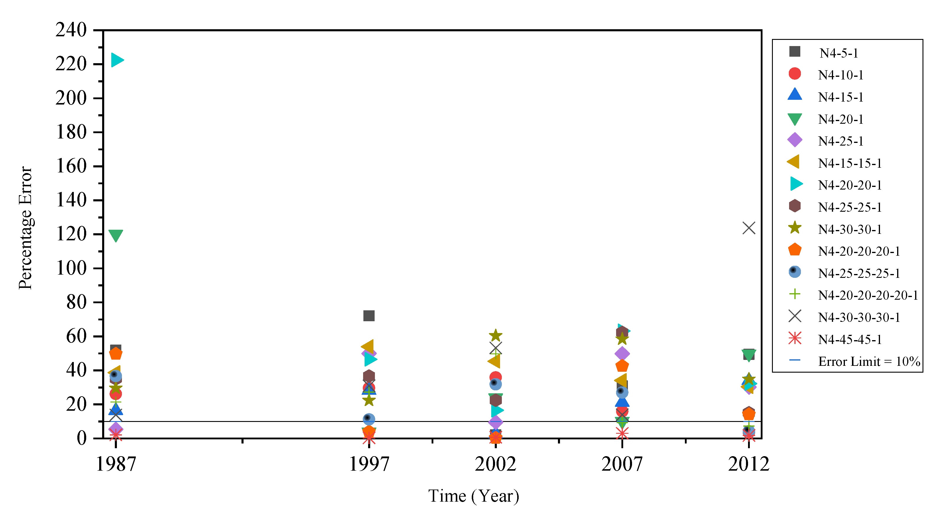
| Nhi-h1-ho | N stands for ANN architecture, hi = number of neurons in the input layer h1 = number of neurons in the hidden layer ho = number of neurons in the output layer |
| Nhi-h1-h2-ho | N stands for ANN architecture, hi = number of neurons in the input layer h1 = number of neurons in the first hidden layer h2 = number of neurons in the second hidden layer ho = number of neurons in the output layer |
| Nhi-h1-h2-h3-ho | N stands for ANN architecture hi = number of neurons in the input layer h1 = number of neurons in the first hidden layer h2 = number of neurons in the second hidden layer h3 = number of neurons in the third hidden layer ho = number of neurons in the output layer |
| R | Correlation Coefficient |
| R.E. | Relative Error |
References
- Pritchard, S. Overlaoded-International Water Power Dam Construction. Progress. Media Int. 2002, 54, 18–22. [Google Scholar]
- Abid, M.; Muftooh, U.R.; Adnan, A.N. Water and Sediment Flow Simulations for Tarbela Reservoir and Tunnels, a Preliminary Study. VDM Verlag Dr. Muler. printed in the U.S.A. and in the U.K.. 2011. Available online: https://www.amazon.com/Sediment-Simulations-Tarbela-Reservoir-Tunnels/dp/363934183X (accessed on 1 August 2022).
- Abid, M.; Muftooh, U.R.S. Multiphase Flow Simulations through Tarbela Dam Spillways and Tunnels. J. Water Resour. Prot. 2010, 2, 532–539. [Google Scholar] [CrossRef] [Green Version]
- Water and Power Development Authority (WAPDA). Tarbela Reservoir Sedimentation Report; WAPDA: Lahore, Pakistan, 2019. [Google Scholar]
- Consultants, Ghazi–Garriala Hydropower (G.G.H). Technical Report No. 3, Sedimentology of Ghazi-Garriala Hydropower Project, Feasibility Report; Water & Power Development Authority: Lahore, Pakistan, 1991. [Google Scholar]
- Consultants, D.B. Reservoir Sedimentation Studies, Appendix C to Reservoir Operation and Sediment Transport; Water and Power Development Authority: Pakistan, Lahore, 2007. [Google Scholar]
- Roca, M. Tarbela Dam in Pakistan. Case Study of Reservoir Sedimentation. In Proceedings of the River Flow, San José, Costa Rica, 5–7 September 2012; Available online: http://eprints.hrwallingford.com/id/eprint/891 (accessed on 15 August 2022).
- Abrahat, R.J.; White, S.M. Modelling sediment transfer in Malawi: Comparing backpropagation neural network solutions against a multiple linear regression benchmark using small data sets. Phys. Chem. Earth Part B Hydrol. Ocean. Atmos. 2001, 26, 19–24. [Google Scholar] [CrossRef]
- Cigizoglu, H.K. Suspended Sediment Estimation and Forecasting using Artificial Neural Networks. Turkish J. Eng. Env. Sci. 2002, 26, 15–25. [Google Scholar]
- Cigizoglu, H.K. Suspended Sediment Estimation for Rivers using Artificial Neural Networks and Sediment Rating Curves. Turkish J. Eng. Env. Sci. 2002, 26, 27–36. [Google Scholar]
- Dibike, Y.B.; Solomatine, D.; Abbott, M.B. On encapsulation of numeric–hydraulic models in artificial neural networks. J. Hyd. Res. 2010, 37, 147–161. [Google Scholar] [CrossRef]
- Li, X.; Qiu, J.; Shang, Q.; Li, F. Simulation of Reservoir Sediment Flushing of the Three Gorges Reservoir Using an Artificial Neural Network. Appl. Sci. 2016, 6, 148. [Google Scholar] [CrossRef] [Green Version]
- Tarar, Z.R.; Ahmad, S.R.; Ahmad, I.; Hasson, S.U.; Khan, Z.M.; Washakh, R.M.A.; Ateeq-Ur-Rehman, S.; Bui, M.D. Effect of Sediment Load Boundary Conditions in Predicting Sediment Delta of Tarbela Reservoir in Pakistan. Water 2019, 11, 1716. [Google Scholar] [CrossRef] [Green Version]
- Rashid, M.U.; Shakir, A.S.; Khan, N.M. Evaluation of Sediment Management Options and Minimum Operation Levels for Tarbela Reservoir, Pakistan. Arabian J. Sci. Eng. 2014, 39, 2655–2668. [Google Scholar] [CrossRef]
- Petkovsek, G.; Roca, M. Impact of Reservoir Operation on Sediment Deposition. Proceedings of ICE-Water Management. Thomas Telford Ltd. 2014, 167, 577–584. [Google Scholar] [CrossRef] [Green Version]
- Khan, N.M.; Tingsanchali, T. Optimization and simulation of reservoir operation with sediment evacuation: A case study of the Tarbela Dam, Pakistan. Hydrol. Proc. 2009, 23, 730–747. [Google Scholar] [CrossRef]
- Arfan, M.; Lund, J.; Hassan, D.; Saleem, M.; Ahmad, A. Assessment of Spatial and Temporal Flow Variability of the Indus River. Resources 2019, 8, 103. [Google Scholar] [CrossRef] [Green Version]
- Ul Hussan, W.; Khurram Shahzad, M.; Seidel, F.; Costa, A.; Nestmann, F. Comparative Assessment of Spatial Variability and Trends of Flows and Sediments under the Impact of Climate Change in the Upper Indus Basin. Water 2020, 12, 730. [Google Scholar] [CrossRef]
- Chiang, Y.M.; Chang, L.C.; Chang, F.J. Comparison of static-feedforward and dynamic-feedback neural networks for rainfall–runoff modeling. J. Hydr. 2004, 290, 297–311. [Google Scholar] [CrossRef]
- Attewill, L.J.S.; White, W.R.; Tariq, S.M.; Bilgi, A. Sediment management studies of Tarbela dam, Pakistan. In The prospect for reservoirs in the 21st century, Proceedings of the 10th Conference of the British Dam Society, Bangor, UK, 9–12 September 1998; Thomas Telford Publishing: London, UK, 1998; pp. 212–225. [Google Scholar]
- Axel, R.; Rafael, M.C. Performance evaluation of hydrological models: Statistical significance for reducing subjectivity in goodness-of-fit assessments. J. Hydrol. 2013, 480, 33–45. [Google Scholar] [CrossRef]
- Gusarov, A.V.; Sharifullin, A.G.; Beylich, A.A. Contemporary Trends in River Flow, Suspended Sediment Load, and Soil/Gully Erosion in the South of the Boreal Forest Zone of European Russia: The Vyatka River Basin. Water 2021, 13, 2567. [Google Scholar] [CrossRef]
- Török, G.T.; Baranya, S.; Rüther, N. 3D CFD Modeling of Local Scouring, Bed Armoring and Sediment Deposition. Water 2017, 9, 56. [Google Scholar] [CrossRef] [Green Version]
- Rodríguez-Blanco, M.L.; Arias, R.; Taboada-Castro, M.M.; Nunes, J.P.; Keizer, J.J.; Taboada-Castro, M.T. Potential Impact of Climate Change on Suspended Sediment Yield in NW Spain: A Case Study on the Corbeira Catchment. Water 2016, 8, 444. [Google Scholar] [CrossRef] [Green Version]
- Di Francesco, S.; Biscarini, C.; Manciola, P. Characterization of a Flood Event through a Sediment Analysis: The Tescio River Case Study. Water 2016, 8, 308. [Google Scholar] [CrossRef] [Green Version]
- Xiao, L.; Yang, X.; Cai, H. Responses of Sediment Yield to Vegetation Cover Changes in the Poyang Lake Drainage Area, China. Water 2016, 8, 114. [Google Scholar] [CrossRef] [Green Version]
- Yang, X.; Mao, Z.; Huang, H.; Zhu, Q. Using GOCI Retrieval Data to Initialize and Validate a Sediment Transport Model for Monitoring Diurnal Variation of SSC in Hangzhou Bay, China. Water 2016, 8, 108. [Google Scholar] [CrossRef] [Green Version]
- Tfwala, S.S.; Wang, Y.-M. Estimating Sediment Discharge Using Sediment Rating Curves and Artificial Neural Networks in the Shiwen River, Taiwan. Water 2016, 8, 53. [Google Scholar] [CrossRef] [Green Version]
- Guerrero, M.; Rüther, N.; Szupiany, R.; Haun, S.; Baranya, S.; Latosinski, F. The Acoustic Properties of Suspended Sediment in Large Rivers: Consequences on ADCP Methods Applicability. Water 2016, 8, 13. [Google Scholar] [CrossRef]
- Yin, D.; Xue, Z.G.; Gochis, D.J.; Yu, W.; Morales, M.; Rafieeinasab, A. A Process-Based, Fully Distributed Soil Erosion and Sediment Transport Model for WRF-Hydro. Water 2020, 12, 1840. [Google Scholar] [CrossRef]
- Nabi, G.; Hussain, F.; Wu, R.-S.; Nangia, V.; Bibi, R. Micro-Watershed Management for Erosion Control Using Soil and Water Conservation Structures and SWAT Modeling. Water 2020, 12, 1439. [Google Scholar] [CrossRef]
- Németová, Z.; Honek, D.; Kohnová, S.; Hlavčová, K.; Šulc Michalková, M.; Sočuvka, V.; Velísková, Y. Validation of the EROSION-3D Model through Measured Bathymetric Sediments. Water 2020, 12, 1082. [Google Scholar] [CrossRef]
- Luffman, I.; Nandi, A. Seasonal Precipitation Variability and Gully Erosion in Southeastern USA. Water 2020, 12, 925. [Google Scholar] [CrossRef] [Green Version]
- Tavelli, M.; Piccolroaz, S.; Stradiotti, G.; Pisaturo, G.R.; Righetti, M. A New Mass-Conservative, Two-Dimensional, Semi-Implicit Numerical Scheme for the Solution of the Navier-Stokes Equations in Gravel Bed Rivers with Erodible Fine Sediments. Water 2020, 12, 690. [Google Scholar] [CrossRef] [Green Version]
- Kaffas, K.; Saridakis, M.; Spiliotis, M.; Hrissanthou, V.; Righetti, M. A Fuzzy Transformation of the Classic Stream Sediment Transport Formula of Yang. Water 2020, 12, 257. [Google Scholar] [CrossRef] [Green Version]
- Xin, Y.; Xie, Y.; Liu, Y. Effects of Residue Cover on Infiltration Process of the Black Soil under Rainfall Simulations. Water 2019, 11, 2593. [Google Scholar] [CrossRef] [Green Version]
- Al Sayah, M.J.; Nedjai, R.; Kaffas, K.; Abdallah, C.; Khouri, M. Assessing the Impact of Man–Made Ponds on Soil Erosion and Sediment Transport in Limnological Basins. Water 2019, 11, 2526. [Google Scholar] [CrossRef] [Green Version]
- Wang, G.; Tian, S.; Hu, B.; Xu, Z.; Chen, J.; Kong, X. Evolution Pattern of Tailings Flow from Dam Failure and the Buffering Effect of Debris Blocking Dams. Water 2019, 11, 2388. [Google Scholar] [CrossRef] [Green Version]
- Lu, C.M.; Chiang, L.C. Assessment of Sediment Transport Functions with the Modified SWAT-Twn Model for a Taiwanese Small Mountainous Watershed. Water 2019, 11, 1749. [Google Scholar] [CrossRef]
- Song, Y.H.; Yun, R.; Lee, E.H.; Lee, J.H. Predicting Sedimentation in Urban Sewer Conduits. Water 2018, 10, 462. [Google Scholar] [CrossRef] [Green Version]
- Aksoy, H.; Mahe, G.; Meddi, M. Modeling and Practice of Erosion and Sediment Transport under Change. Water 2019, 11, 1665. [Google Scholar] [CrossRef] [Green Version]
- Hauer, C. Sediment Management: Hydropower Improvement and Habitat Evaluation. Water 2020, 12, 3470. [Google Scholar] [CrossRef]
- Patil, M.P.; Jeong, I.; Woo, H.-E.; Oh, S.-J.; Kim, H.C.; Kim, K.; Nakashita, S.; Kim, K. Effect of Bacillus subtilis Zeolite Used for Sediment Remediation on Sulfide, Phosphate, and Nitrogen Control in a Microcosm. Int. J. Environ. Res. Public Health 2022, 19, 4163. [Google Scholar] [CrossRef] [PubMed]
- Reisenbüchler, M.; Bui, M.D.; Skublics, D.; Rutschmann, P. Sediment Management at Run-of-River Reservoirs Using Numerical Modelling. Water 2020, 12, 249. [Google Scholar] [CrossRef] [Green Version]
- Sotiri, K.; Hilgert, S.; Duraes, M.; Armindo, R.A.; Wolf, N.; Scheer, M.B.; Kishi, R.; Pakzad, K.; Fuchs, S. To What Extent Can a Sediment Yield Model Be Trusted? A Case Study from the Passaúna Catchment. Brazil. Water 2021, 13, 1045. [Google Scholar] [CrossRef]
- Jothiprakash, V.; Garg, V. Reservoir Sedimentation Estimation Using Artificial Neural Network. J. Hydrol. Eng. 2009, 14, 1035–1040. [Google Scholar] [CrossRef]
- Chen, S.L.; Zhang, G.A.; Young, S.L.; Shi, J.Z. Temporal variations of fine suspended sediment concentration in the Changjiang River estuary and adjacent coastal waters, China. J. Hydrol. 2006, 331, 137–145. [Google Scholar] [CrossRef]
- Wang, Y.M.; Tfwala, S.S.; Chan, H.C.; Lin, Y.C. The effects of sporadic torrential rainfall events on suspended sediments. Arch. Sci. J. 2013, 66, 211–224. [Google Scholar]
- Teng, W.-H.; Hsu, M.-H.; Wu, C.-H.; Chen, A.S. Impact of flood disasters on Taiwan in the last quarter century. Nat. Hazards 2006, 37, 191–207. [Google Scholar] [CrossRef] [Green Version]
- Milliman, J.D.; Syvitski, J.P. Geomorphic/tectonic control of sediment discharge to the ocean: The importance of small mountainous rivers. J. Geol. 1992, 100, 525–544. [Google Scholar] [CrossRef]
- Horowitz, A.J. An evaluation of sediment rating curves for estimating suspended sediment concentrations for subsequent flux calculations. Hydrol. Process. 2003, 17, 3387–3409. [Google Scholar] [CrossRef]
- Thomas, R.B. Estimating total suspended sediment yield with probability sampling. Water Resour. Res. 1985, 21, 1381–1388. [Google Scholar] [CrossRef] [Green Version]
- Wang, Y.M.; Traore, S. Time-lagged recurrent network for forecasting episodic event suspended sediment load in typhoon prone area. Int. J. Phys. Sci. 2009, 4, 519–528. [Google Scholar]
- Chen, S.M.; Wang, Y.M.; Tsou, I. Using artificial neural network approach for modelling rainfall–runoff due to typhoon. J. Earth Syst. Sci. 2013, 122, 399–405. [Google Scholar] [CrossRef] [Green Version]
- Tfwala, S.S.; Wang, Y.M.; Lin, Y.C. Prediction of missing flow records using multilayer perceptron and coactive neurofuzzy inference system. Sci. World J. 2013, 2013, 584516. [Google Scholar] [CrossRef] [Green Version]
- Melesse, A.M.; Ahmad, S.; McClain, M.E.; Wang, X.; Lim, Y.H. Suspended sediment load prediction of river systems: An artificial neural network approach. Agric. Water Manag. 2011, 98, 855–866. [Google Scholar] [CrossRef]
- Kisi, O. Generalized regression neural networks for evapotranspiration modelling. Hydrol. Sci. J. 2006, 51, 1092–1105. [Google Scholar] [CrossRef]
- Wang, Y.M.; Traore, S.; Kerh, T. Computing and modelling for crop yields in burkina faso based on climatic data information. WSEAS Trans. Inf. Sci. Appl. 2008, 5, 832–842. [Google Scholar]
- Lin, J.Y.; Cheng, C.T.; Chau, K.W. Using support vector machines for long-term discharge prediction. Hydrol. Sci. J. 2006, 51, 599–612. [Google Scholar] [CrossRef]
- Leahy, P.; Kiely, G.; Corcoran, G. Structural optimisation and input selection of an artificial neural network for river level prediction. J. Hydrol. 2008, 355, 192–201. [Google Scholar] [CrossRef]
- Martens, J.; Sutskever, I. Learning Recurrent Neural Networks with Hessian-Free Optimization. In Proceedings of the 28th International Conference on Machine Learning, Bellevue, WA, USA, 28 June–2 July 2011. [Google Scholar]
- Feyzolahpour, M.; Rajabi, M.; Roostaei, S. Estimating suspended sediment concentration using neural differential evolution (NDE), multilayer perceptron (MLP) and radial basis function (RBF) models. Int. J. Phys. Sci. 2012, 7, 5106–5177. [Google Scholar] [CrossRef]
- Zhang, X.; Yang, Y. Suspended sediment concentration forecast based on CEEMDAN-GRU model. Water Supply 2020, 20, 1787–1798. [Google Scholar] [CrossRef]
- Froehlich, D.C.; Giri, S. Neural Network Prediction of Reservoir Sedimentation. In Proceedings of the 14th International Symposium on River Sedimentation, Chengdu, China, 16–19 September 2019. [Google Scholar] [CrossRef]
- Uca; Toriman, E.; Jaafar, O.; Maru, R.; Arfan, A.; Ahmar, A.S. Daily Suspended Sediment Discharge Prediction Using Multiple Linear Regression and Artificial Neural Network. J. Phys. 2018, 954, 012030. [Google Scholar] [CrossRef] [Green Version]
- Nourani, V. Using Artificial Neural Networks (ANNS) for Sediment Load Forecasting of Talkherood River Mouth. J. Urb. Env. Eng. 2009, 3, 1–6. Available online: http://www.jstor.org/stable/26203327 (accessed on 21 September 2022). [CrossRef]
- Sokchhay, H.; Tadashi, S. Using Artificial Neural Network to Estimate Sediment Load in Ungauged Catchments of the Tonle Sap River Basin, Cambodia. J. Water Resour. Prot. 2013, 5, 111–123. [Google Scholar] [CrossRef] [Green Version]
- Qian, L.; Liu, C.; Yi, J.; Liu, S. Application of hybrid algorithm of bionic heuristic and machine learning in nonlinear sequence. J. Phys. Conf. Ser. 2020, 1682, 012009. [Google Scholar] [CrossRef]
- Fallah, S.N.; Deo, R.C.; Shojafar, M.; Conti, M.; Shamshirband, S. Computational intelligence approaches for energy load forecasting in smart energy management grids: State of the art, future challenges, and research directions. Energies 2018, 11, 596. [Google Scholar] [CrossRef] [Green Version]
- Kabir, S.; Patidar, S.; Xi, X.; Liang, Q.; Neal, J.; Pender, G. A deep convolutional neural network model for rapid prediction of fluvial food inundation. J. Hydrol. 2020, 590, 125481. [Google Scholar] [CrossRef]
- Haurum, J.B.; Bahnsen, C.H.; Pedersen, M.; Moeslund, T.B. Water Level Estimation in Sewer Pipes Using Deep Convolutional Neural Networks. Water 2020, 12, 3412. [Google Scholar] [CrossRef]
- Ni, C.; Ma, X. Prediction of Wave Power Generation Using a Convolutional Neural Network with Multiple Inputs. Energies 2018, 11, 2097. [Google Scholar] [CrossRef] [Green Version]
- Samantaray, S.; Sahoo, A. Prediction of suspended sediment concentration using hybrid SVM-WOA approaches. Geocarto Int. 2022, 19, 5609–5635. [Google Scholar] [CrossRef]
- Nouar, A.; Yusuf, E.; Pavitra, K.; Ali, N.A.; Mohsen, S.; Ahmed, S.; Ahmed, E. Suspended sediment load prediction using long short-term memory neural network. Sci. Rep. 2021, 11, 7826. [Google Scholar] [CrossRef]
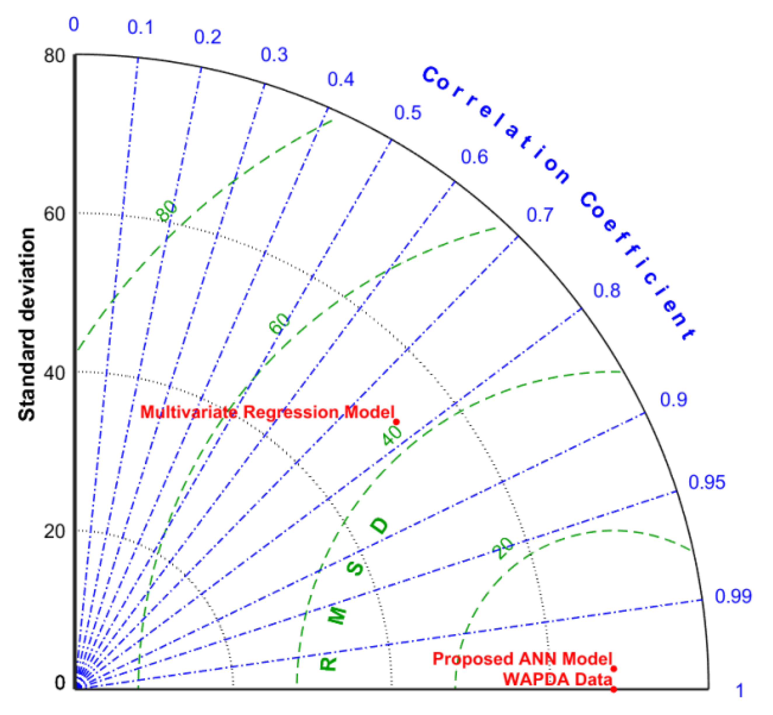
- Taylor, K.E. Summarizing multiple aspects of model performance in a single diagram. J. Geophys. Res. 2001, 106, 7183–7192. [Google Scholar] [CrossRef]
- Olden, J.D.; Joy, M.K.; Death, R.G. An accurate comparison of methods for quantifying variable importance in artificial neural networks using simulated data. Ecol. Mod. 2004, 178, 389–397. [Google Scholar] [CrossRef]


| Parameter | Value |
|---|---|
| Batch size | 100 |
| Learning rate | 0.001 |
| The number of hidden layers | 2 |
| The number of neurons at kth hidden layer | 45 |
| The number of neurons at input layer | 4 |
| The number of neurons at output layer | 1 |
| Activation function | Sigmoid |
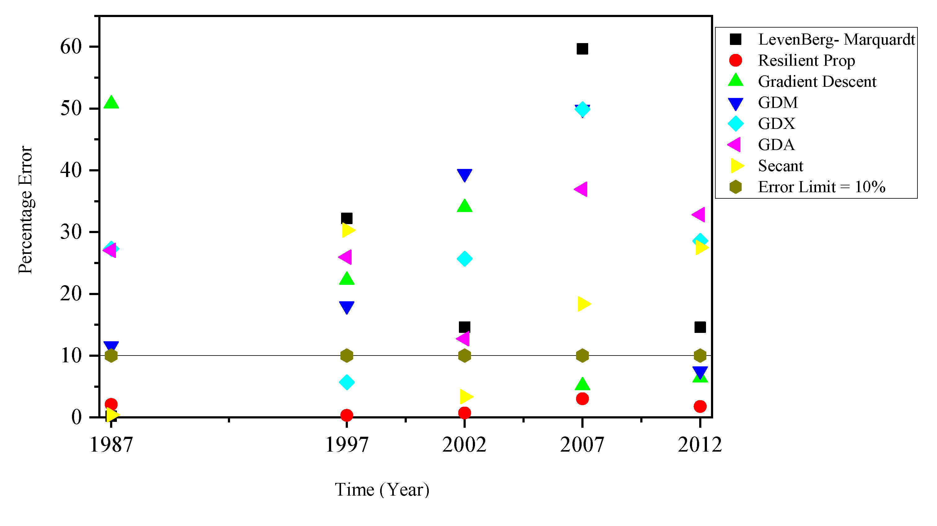
| Training Function | trainrp |
| Optimizer | Adam |
| Epoch | 20 |
| Regularization | L1 (Lasso regression) |
| Problem type | Time Series (Sequential) |
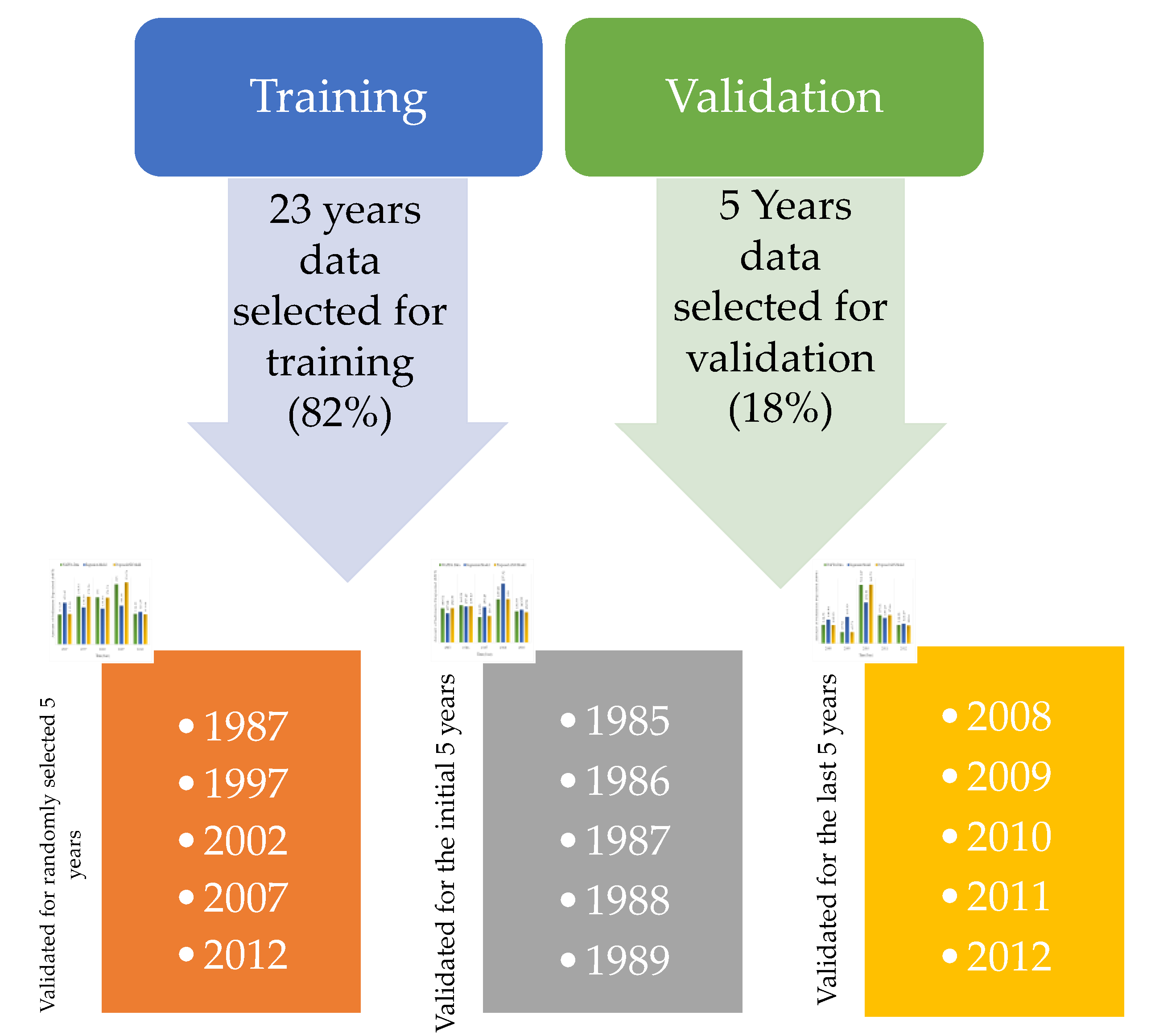
| Ratio of training to test data (%) | 82:18 |
| Variables | p | q | r | s | Intercept |
|---|---|---|---|---|---|
| Ra only | 0.073212 | 0 | 0 | 0 | 84.17088 |
| Iw only | 0 | 0.00522 | 0 | 0 | −218.58 |
| LR only | 0 | 0 | −0.10758 | 0 | 224.7589 |
| Cr only | 0 | 0 | 0 | −0.00339 | 217.077 |
| Ra and Iw | 0.00575 | −0.04186 | 0 | 0 | −199.299 |
| Iw and Lr | 0 | 0.005683 | −1.32448 | 0 | 299.2509 |
| Lr and Cr | 0 | 0 | −0.12451 | −0.00345 | 270.0721 |
| Iw and Cr | 0 | 0.005295 | 0 | −0.00513 | −162.88 |
| Ra, Iw, and Lr | −0.04103 | 0.006149 | 1.3160 | 0 | 314.409 |
| Ra, Lr, and Cr | 0.0977 | 0 | 0.42128 | 0.01152 | 354.270 |
| Iw, Lr, and Cr | 0 | 0.005721 | 1.36206 | 0.00601 | 378.5874 |
| All Parameters | −0.033 | 0.6 | −1.34 | −0.34 | 356.96 |
| Performance Metrics | Randomly Selected 5 Years Data Set | Initial 5 Years Data Set | Last 5 Years Data Set |
|---|---|---|---|
| MSE | 0.000529 | 0.00539 | 0.000166 |
| MAE | 0.017604 | 0.019629 | 0.015607 |
| R-Training | 0.99928 | 0.997 | 1 |
| R-Validation | 0.99823 | 0.991 | 0.99902 |
| NSE | 0.99436 | 0.98271 | 0.99965 |
| Minimum Gradient | 9.79 × 10⁻⁷ | 9.18 × 10⁻⁷ | 9.97 × 10⁻⁷ |
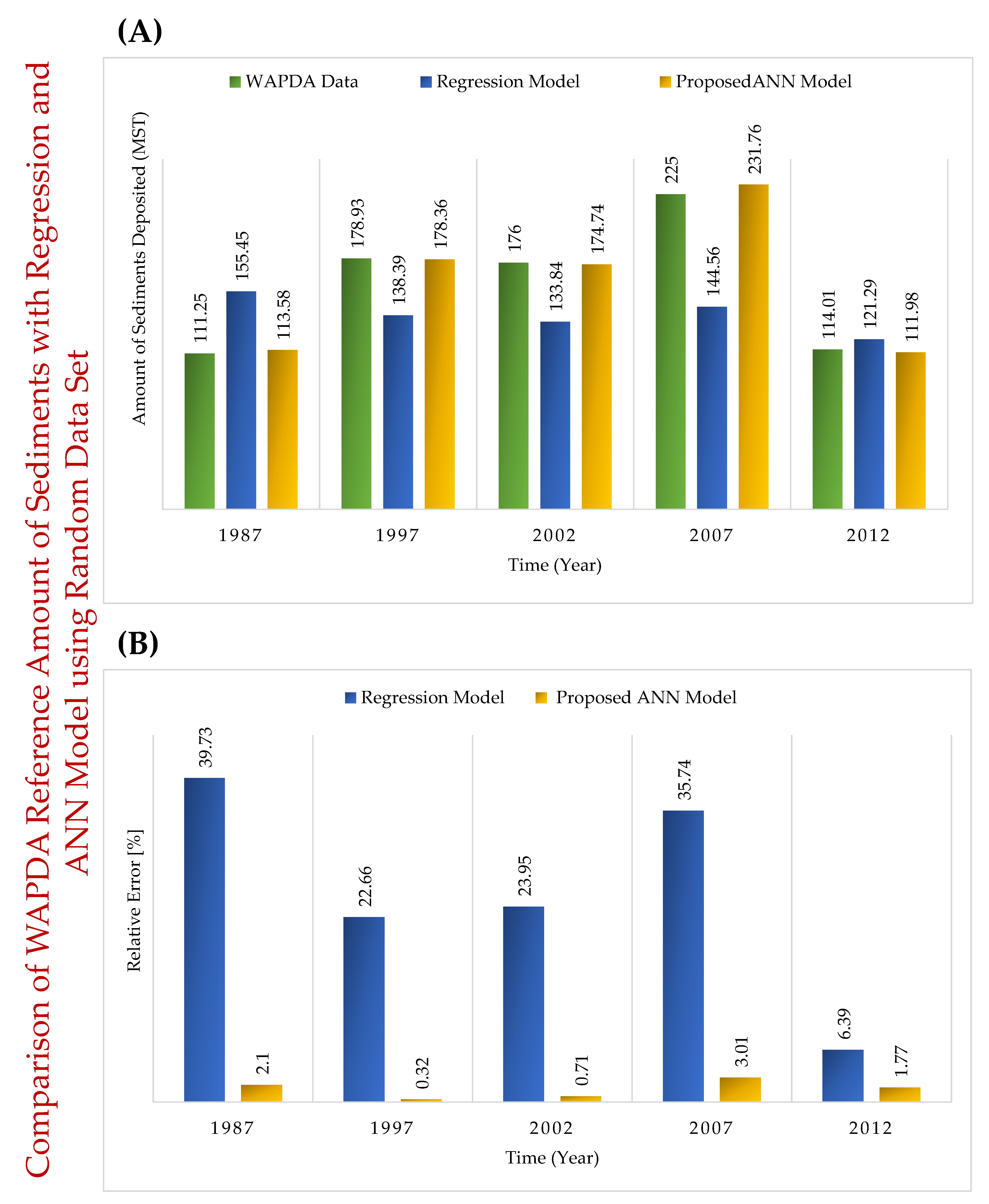
| Year | Randomly Selected 5 Years Data Set | Initial 5 Years Data Set [R.E. (%)] | Last 5 Years Data Set [R.E. (%)] |
|---|---|---|---|
| 1987 | 111.25 | 155.45 [39.73] | 113.58 [2.10] |
| 1997 | 178.93 | 138.39 [22.66] | 178.36 [0.32] |
| 2002 | 176 | 133.84 [23.95] | 174.74 [0.71] |
| 2007 | 225 | 144.56 [35.74] | 231.76 [3.01] |
| 2012 | 114.01 | 121.29 [6.39] | 111.98 [1.77] |
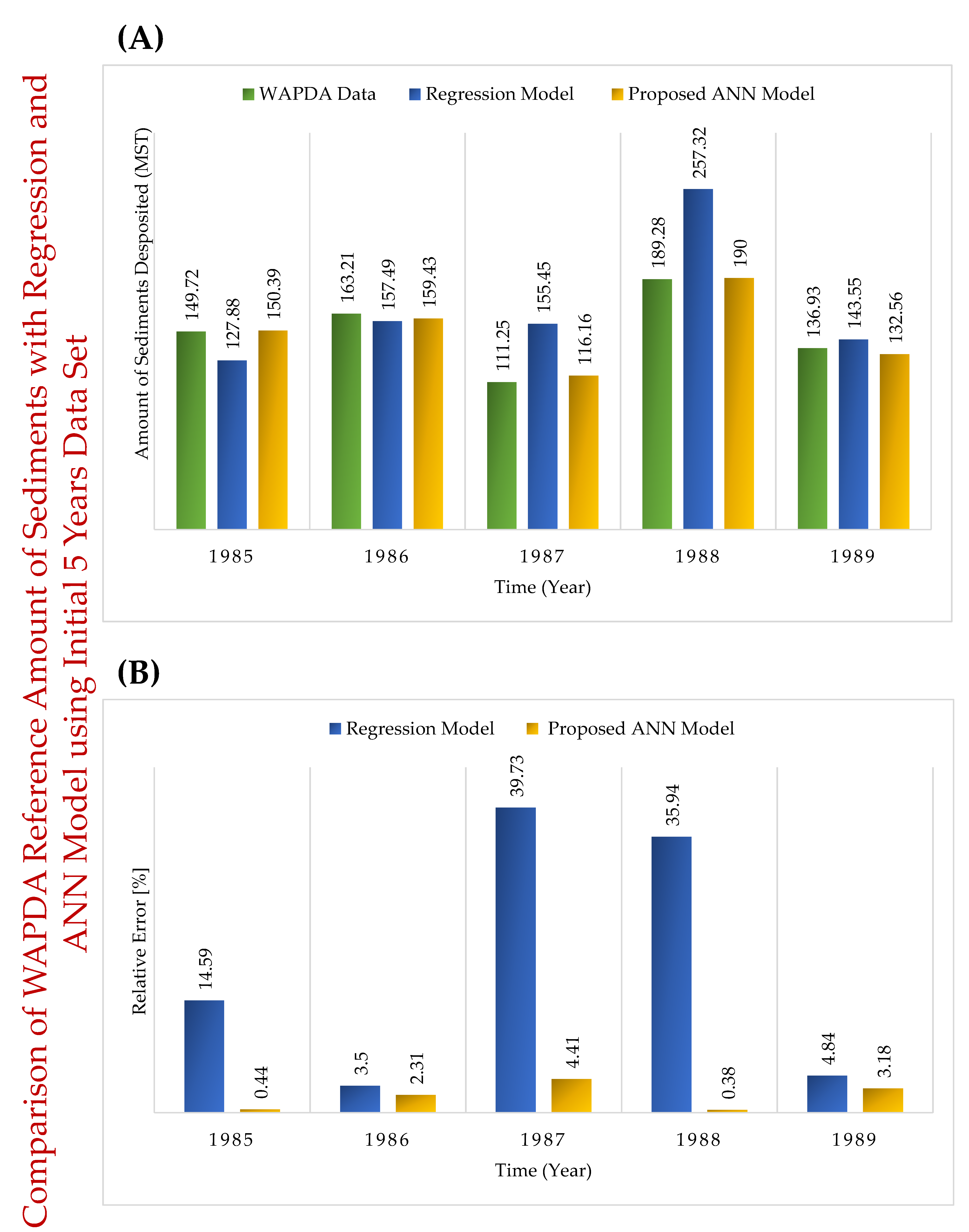
| Year | Randomly Selected 5 Years Data Set | Initial 5 Years Data Set [R.E. (%)] | Last 5 Years Data Set [R.E. (%)] |
|---|---|---|---|
| 1985 | 149.72 | 127.88 [14.59] | 150.39 [0.44] |
| 1986 | 163.21 | 157.49 [3.5] | 159.43 [2.31] |
| 1987 | 111.25 | 155.45 [39.73] | 116.16 [4.41] |
| 1988 | 189.28 | 257.32 [35.94] | 190 [0.38] |
| 1989 | 136.93 | 143.55 [4.84] | 132.56 [3.18] |
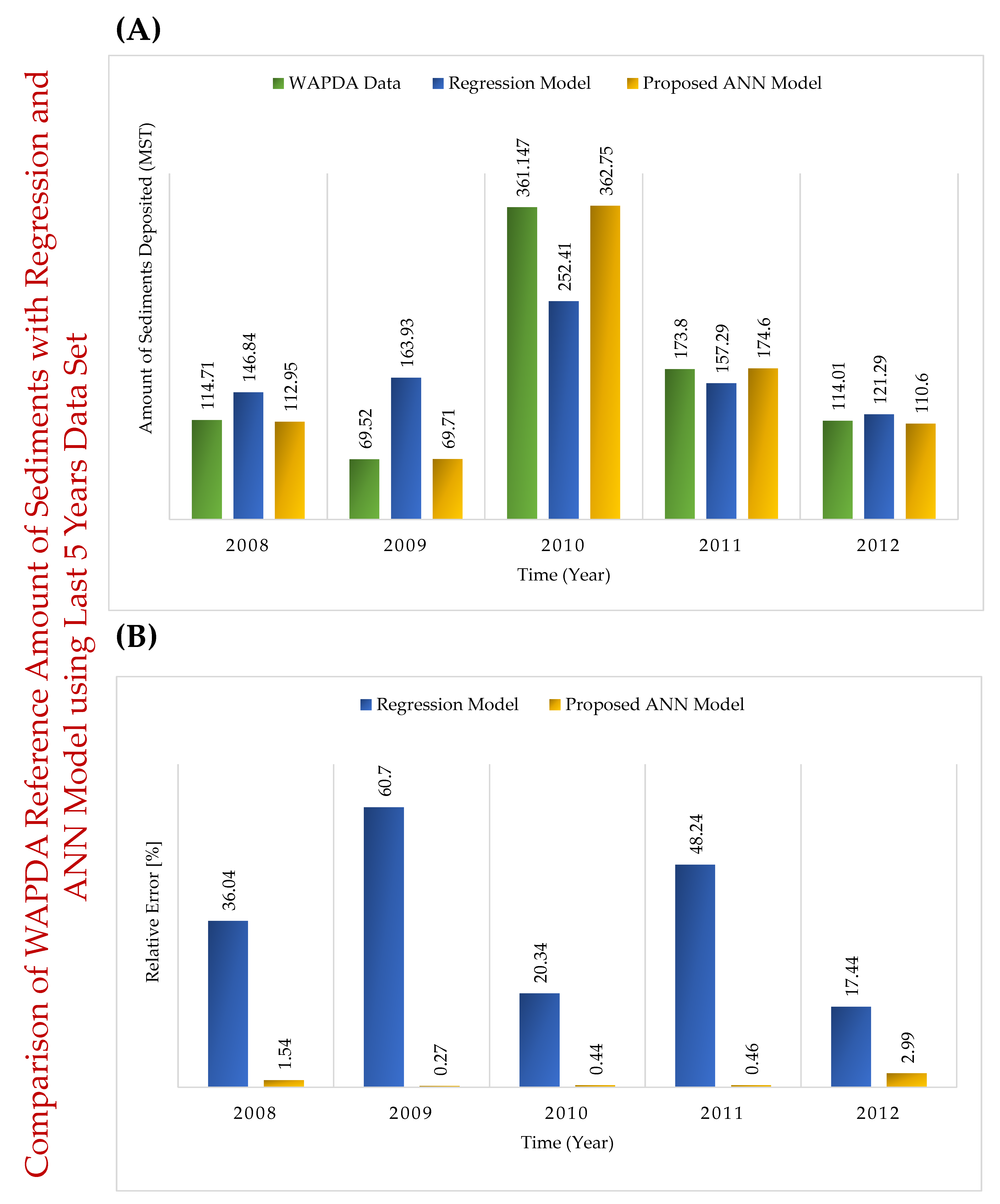
| Year | WAPDA Data (MST) | Regression Model (MST) [R.E. (%)] | ANN Model (MST) [R.E. (%)] |
|---|---|---|---|
| 2008 | 114.71 | 146.84 [36.04] | 112.95 [1.54] |
| 2009 | 69.52 | 163.93 [60.7] | 69.71 [0.27] |
| 2010 | 361.147 | 252.41 [20.34] | 362.75 [0.44] |
| 2011 | 173.8 | 157.29 [48.24] | 174.6 [0.46] |
| 2012 | 114.01 | 121.29 [17.44] | 110.6 [2.99] |
Publisher’s Note: MDPI stays neutral with regard to jurisdictional claims in published maps and institutional affiliations. |
© 2022 by the authors. Licensee MDPI, Basel, Switzerland. This article is an open access article distributed under the terms and conditions of the Creative Commons Attribution (CC BY) license (https://creativecommons.org/licenses/by/4.0/).
Share and Cite
Hassan, S.; Shaukat, N.; Ahmad, A.; Abid, M.; Hashmi, A.; Shahid, M.L.U.R.; Rajabi, Z.; Tariq, M.A.U.R. Prediction of the Amount of Sediment Deposition in Tarbela Reservoir Using Machine Learning Approaches. Water 2022, 14, 3098. https://doi.org/10.3390/w14193098
Hassan S, Shaukat N, Ahmad A, Abid M, Hashmi A, Shahid MLUR, Rajabi Z, Tariq MAUR. Prediction of the Amount of Sediment Deposition in Tarbela Reservoir Using Machine Learning Approaches. Water. 2022; 14(19):3098. https://doi.org/10.3390/w14193098
Chicago/Turabian StyleHassan, Shahzal, Nadeem Shaukat, Ammar Ahmad, Muhammad Abid, Abrar Hashmi, Muhammad Laiq Ur Rahman Shahid, Zohreh Rajabi, and Muhammad Atiq Ur Rehman Tariq. 2022. "Prediction of the Amount of Sediment Deposition in Tarbela Reservoir Using Machine Learning Approaches" Water 14, no. 19: 3098. https://doi.org/10.3390/w14193098