A Simulation Study Using Machine Learning and Formula Methods to Assess the Soybean Groundwater Contribution in a Drought-Prone Region

Abstract

Groundwater contributes to the delivery of phreatic water to crop aeration zones via evapotranspiration, which is important for crop growth in drought-prone regions. Most studies on groundwater contribution have not considered the influence of crop growth stage or daily evapotranspiration. In this study, a neural network based on a genetic algorithm and the Levenberg–Marquardt backpropagation algorithm, as well as formula methods based on an accelerated genetic algorithm, were built to assess soybean groundwater contribution; in addition, a performance comparison was conducted. The results indicated that machine learning had the best performance for fitting errors, with values for relative mean error (RME), root mean square percentage error (RMSPE), and correlation coefficient of 1.088, 2.165, and 0.762, respectively; in addition, for validation errors, it had values for RME, RMSPE, and correlation coefficient of 1.069, 2.136, and 0.735, respectively. The machine learning method is recommended for readers seeking to calculate groundwater contribution.

1. Introduction

The groundwater contribution of growing crops occurs through phreatic evaporation [1,2]. Crop roots are often above groundwater; the evaporation of groundwater can increase soil moisture, and crop roots can absorb water from soil moisture. Therefore, groundwater is an important water source for crop growth, and the calculation of its contribution is significant for irrigation planning and water resource management [3]. In hydrological models, groundwater is also an important component, and its evaporation affects the modeling of soil moisture [4,5].

It has previously been observed that phreatic evaporation is related to water evaporation capacity and water table depth. Aviriyanover [6] proposed empirical formulae involving groundwater depth, water evaporation capability, and phreatic water evaporation to calculate phreatic evaporation. Subsequently, similar formulae have been developed [7,8,9]. However, these studies did not consider crop growth and could not simulate phreatic evaporation in crops. Therefore, Fidantemiz, et al. [10] used lysimeter experiments to obtain crop water use data and analyzed the relationship between crop water use and groundwater depth. However, they only analyzed qualitative relationships rather than quantitative relationships. Zhou and Wang [11] and Wang, et al. [12] established a quantitative relationship between groundwater contribution and groundwater depth and used Gaussian or quasi-Gaussian functions to fit the scatter of groundwater contribution and groundwater depth; however, they did not consider the influence of meteorological conditions or crop evapotranspiration on the groundwater contribution. As a result, they only fitted the groundwater contribution data on a ten-day or monthly scale. For hydrological models and water resource management, it is very common to use daily scale data for calculation and analysis. Karimov, et al. [13] considered the effect of crop evapotranspiration and fitted the scatter of the ratio of groundwater contribution, crop evapotranspiration, and groundwater depth; however, they did not develop a formula for groundwater contribution. Shah, et al. [14] calculated the crop groundwater contribution for different land cover types and focused on the relationship between the depth to the water table and the ratio of groundwater evapotranspiration to potential evapotranspiration. However, crop water uptake differs because of different root densities in different crop growth stages, and Shah, Nachabe and Ross [14] did not consider the influence of crop growth stages on groundwater contribution.

Therefore, the main issue addressed in this study is the introduction of crop growth stages and crop evapotranspiration into phreatic evaporation formulas to consider the effect of additional factors on groundwater contribution. In addition, we used machine learning in order to find a better simulation model for groundwater contribution, with the values for crop evapotranspiration and groundwater depth fed into the neural network.

Several studies have introduced machine learning for groundwater modeling. They have mainly focused on groundwater-level simulations [15,16,17,18] and groundwater quality evaluations [19,20,21,22]. Previous studies on machine learning have not considered groundwater contribution. In addition, previous studies on groundwater contribution have not considered the influence of crop growth stages or crop evapotranspiration on groundwater contribution.

In this study, to consider the influence of crop growth stages and crop evapotranspiration, machine learning and formula methods based on an accelerated gene algorithm (AGA) were used to simulate soybean groundwater contribution, and their performances were compared. In addition, soybean growth stage was regarded as an important influencing factor, and the relationship between soybean growth stage and groundwater contribution was analyzed.

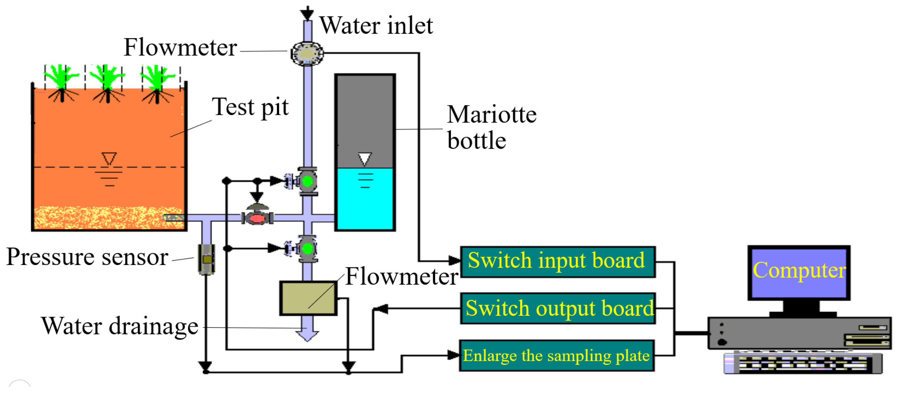
2. Materials and Methods

2.1. Groundwater Contribution of Soybeans

The groundwater contribution of soybeans was estimated using a Mariotte bottle system (Figure 1). The bottles were connected to the crop test pit, and both bottles and pits had the same water table. When the soybeans consumed underground water, the water from the bottle replenished the underground water in the test pit. To maintain the water table at a constant level, water was automatically added to the Mariotte bottle using a pressure sensor and controller, and the value of the groundwater contribution was obtained from the flowmeter and recorded on a computer. In the absence of crops, the groundwater contribution was equal to that of phreatic evaporation.

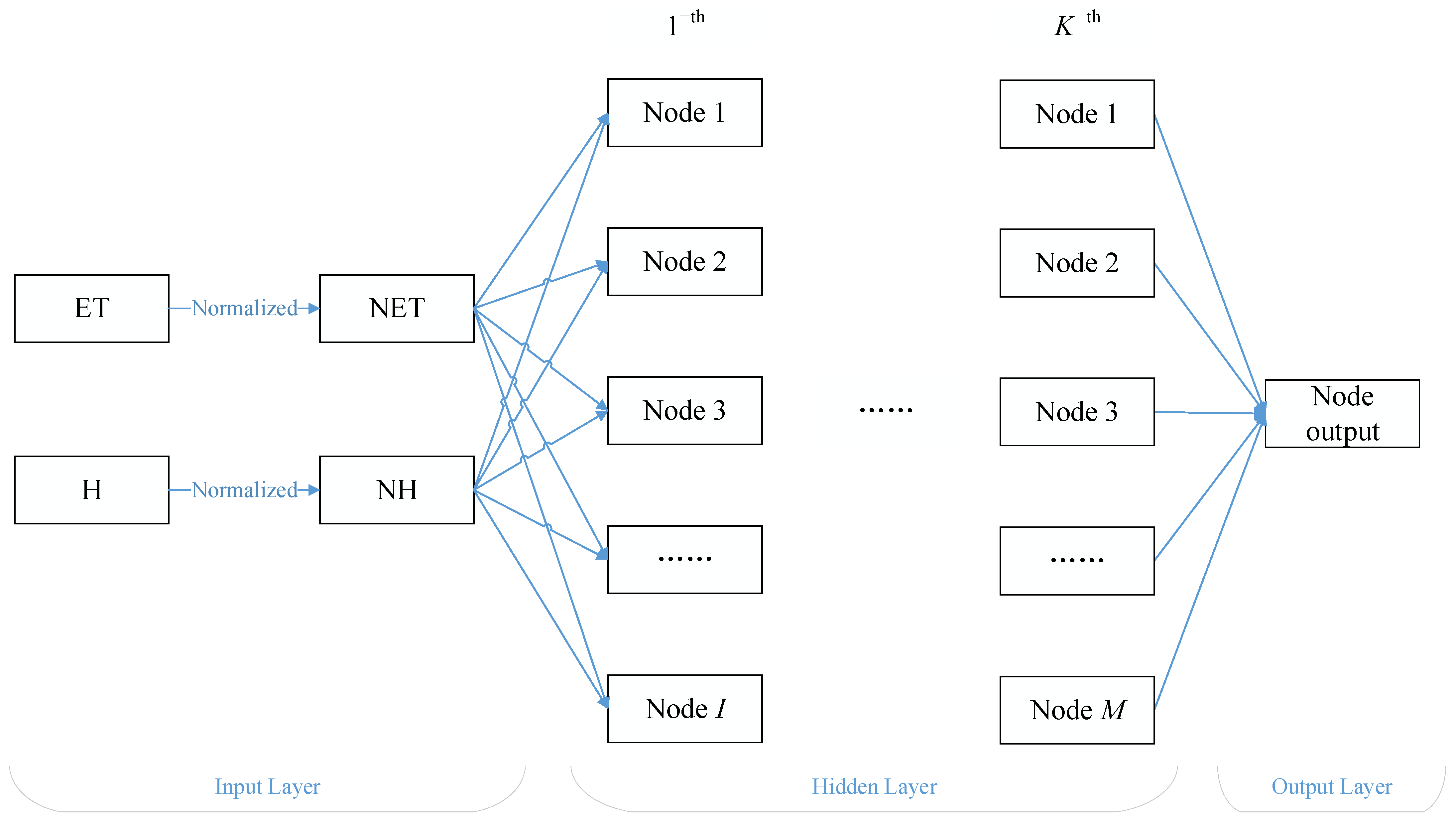
2.1.1. Machine Learning Method

The machine learning method used was a feed-forward model of a neural network with three layers (see Figure 2), which consisted of an input layer, an output layer, and some hidden layers. It was trained using the Levenberg–Marquardt backpropagation algorithm [23], which is the standard backpropagation for supervised learning. The Levenberg–Marquardt algorithm [24] is the fastest method for training moderate-sized feed-forward neural networks but requires more memory than other algorithms. The Levenberg–Marquardt algorithm was used iteratively to minimize the mean square error (MSE) between the output of the ANN and the observation of the groundwater contribution. The iteration process was stopped when the iteration times were larger than a threshold value or when the MSE was below a threshold value.

The structure of the neural network included daily crop evapotranspiration (ET) and groundwater depth (H) in the input layer, which were normalized using Equations (1) and (2). Normalized data were fed into the first hidden layer. There are I nodes in the first hidden layer, and the calculation is shown in Equation (3). All outputs of the I nodes were fed into the second hidden layer, and the results were calculated using Equation (4). Then, the outputs of the k^th hidden layer were fed into the k+1th hidden layer using Equation (4), and there were K hidden layers. Finally, the results were obtained for the output node.

NET = (ET − min (ET))/(max (ET) − min (ET))

(1)

NH = (H − min (H))/(max (H) − min (H))

(2)

$$a_i^1=fun(W_{NET,i}NET+W_{Hi}H+b_i$$

(3)

$$a_m^{k+1}=fun({\displaystyle \sum _{j=1}^J{a}_j^k{W}_j^m+b_m^{k+1})}$$

(4)

where NET is the normalized ET; min (ET) is the minimum value of all the ET data (mm/d); max (ET) is the maximum value of all the ET data (mm/d); NH is the normalized H; $a_i^1$ is the output of node i in the first hidden layer; W_NET,i and W_H,i are the weights of node i for NET and H in the first hidden layer, respectively; b_i is the bias of node i in the first hidden layer; $a_m^{k+1}$ is the output of node m in the k+1^th hidden layer; $W_j^m$ is the weight of node m for $a_j^k$ in the k+1^th hidden layer; $b_m^{k+1}$ is the bias of node m in the k+1^th hidden layer; J is the total number of hidden layers; and fun is an activation function.

A genetic algorithm (GA) was used to optimize the structure of the neural network. The number of nodes and hidden layers are the optimization variables, and Equation (5) is the objective function. The number of nodes ranged from 1 to 7, and the number of hidden layers ranged from 1 to 3. There were six activation functions: the symmetric sigmoid transfer function, the logarithmic sigmoid transfer function, the Elliot sigmoid transfer function, the positive hard limit transfer function, the positive linear transfer function, and the linear transfer function. We tested each activation function and found that the symmetric sigmoid transfer function (Equation (6)) led to the best performance for the neural network. Therefore, Equation (6) was selected as the activation function.

$$\min (1-r^2)=\min \frac{{\displaystyle \sum _{i=1}^m{(x_i-y_i)}^2}}{{\displaystyle \sum _{i=1}^m{(y_i-\overline{y})}^2}}$$

(5)

$$y=\frac{2}{1+e^{-2x}}-1$$

(6)

where x_i is the simulated daily groundwater contribution (mm/d), y_i the observed daily groundwater contribution, r² is the goodness of fit, x is the independent variable of the symmetric sigmoid transfer function, and y is the dependent variable of the symmetric sigmoid transfer function.

2.1.2. Formula Method

In terms of formula methods, there are some formulas for phreatic evaporation, such as those of Aviriyanover and Ye Shuiting, as well as the power function [25]. However, these formulas cannot account for phreatic evaporation with soybean growth, that is, the groundwater contribution of soybeans. To consider the effect of soybean evapotranspiration on groundwater contribution [4], groundwater contribution formulas were built by referring to the phreatic evaporation formulas, in which evaporation capacity was replaced by soybean evapotranspiration. The groundwater contribution is shown in Equations (7)–(9):

(1) The Aviriyanover formula:

$$E_g=E{T}_c{(1-\frac{H}{H_{\max }})}^n$$

(7)

(2) The Ye Shuiting formula:

$$E_g=E{T}_c\cdot {\mathrm{e}}^{-a_1\frac{H}{H_{\max }}}$$

(8)

(3) The power function formula:

$$E_g=a\cdot E{T}_c{(\frac{H}{H_{\max }})}^{-b}$$

(9)

where E_g is the daily groundwater contribution (mm/d); ET_c is the daily soybean evapotranspiration (mm/d) (see the section “Soybean evapotranspiration”); H is groundwater depth (m); H_max is the groundwater depth where the groundwater contribution of soybeans is 0 (m); and n, a₁, a, and b are empirical constants. These empirical constants were optimized using an accelerated genetic algorithm (AGA) [26] and objective Function (5). The ranges of n, a₁, a, and b are 0~7, 0.5~5, 0~1, and 0~3, respectively.

The groundwater contribution data were fitted and validated using machine learning and formula methods, combined with 15 years of recorded data from a test station (Figure 3). The fitting and validation errors were then calculated using Equations (10)–(12). The recommended calculation method can be determined based on the validation results to provide a reference for the calculation of groundwater contribution in the Huaibei Plain.

(1) Relative mean error (RME) [27]:

$$RME=\frac{{\displaystyle \sum _{i=1}^m\frac{|x_i-y_i|}{y_i}}}{m}$$

(10)

(2) Root mean square percentage error (RMSPE) [27]:

$$RMSPE={(\frac{1}{m}{\displaystyle \sum _{i=1}^m{[\frac{x_i-y_i}{y_i}]}^2})}^{0.5}$$

(11)

(3) Correlation coefficient (R) [28]:

$$R=\frac{{\displaystyle \sum _{i=1}^m(x_i-\overline{x})(y_i-\overline{y})}}{\sqrt{{\displaystyle \sum _{i=1}^m{(x_i-\overline{x})}^2}}\sqrt{{\displaystyle \sum _{i=1}^m{(y_i-\overline{y})}^2}}}$$

(12)

where i is the sample number, and i = 1, 2,…, m; m is the total number of groundwater contribution samples; x_i is the calculated value of the groundwater contribution on day i, in mm; y_i is the observed value of the groundwater contribution on day i, in mm; $\overline{x}$ is the average calculated value of the groundwater contribution, in mm; and $\overline{y}$ is the observed average value of the groundwater contribution, in mm.

2.2. Soybean Evapotranspiration

Soybean evapotranspiration values can be obtained by multiplying the reference crop evapotranspiration by the relevant crop factors:

ET_c = K_c × ET₀

(13)

$$E{T}_0=\frac{0.408\Delta (R_n-G)+\gamma \frac{900}{T+273}{U}_2(e_a-e_d)}{\Delta +\gamma (1+0.34U_2)}$$

(14)

where ET_c is daily crop evapotranspiration (mm/d); K_c is a crop coefficient that reveals the relationship parameters between actual crop evapotranspiration and reference crop evapotranspiration (the crop coefficients of soybeans in various growth periods are shown in

Table 1. Crop factors for soybeans.

Crops	Growth Periods	Jan. 1	Feb.	Mar.	Apr.	May	Jun.	July	Aug.	Sep.	Oct.	Nov.	Dec.
Soybean	6.10–9.30 2						0.536	0.909	1.142	1.279

¹ Soybeans do not grow from January to May or from October to December. Therefore, there are no values for some months. ² “6.10–9.30” means that soybeans are in a growth period from 10 June to 30 September.

); ET₀ is the reference crop evapotranspiration (mm/d), which was calculated using the Penman–Monteith formula [29,30] (see Formula (14)); Δ is the slope of the tangent of point T in the relation curve between temperature and saturation vapor pressure (kPa·°C⁻¹); R_n is the net radiance (MJ/m²·d); G is the soil heat flux (MJ/m²·d); γ is the humidity constant (kPa °C⁻¹); T is the average temperature (°C); U₂ is the wind speed at a height of 2 m (m/s); e_a is the saturation vapor pressure (kPa); and e_d is the actual water pressure (kPa).

3. Results and Discussion

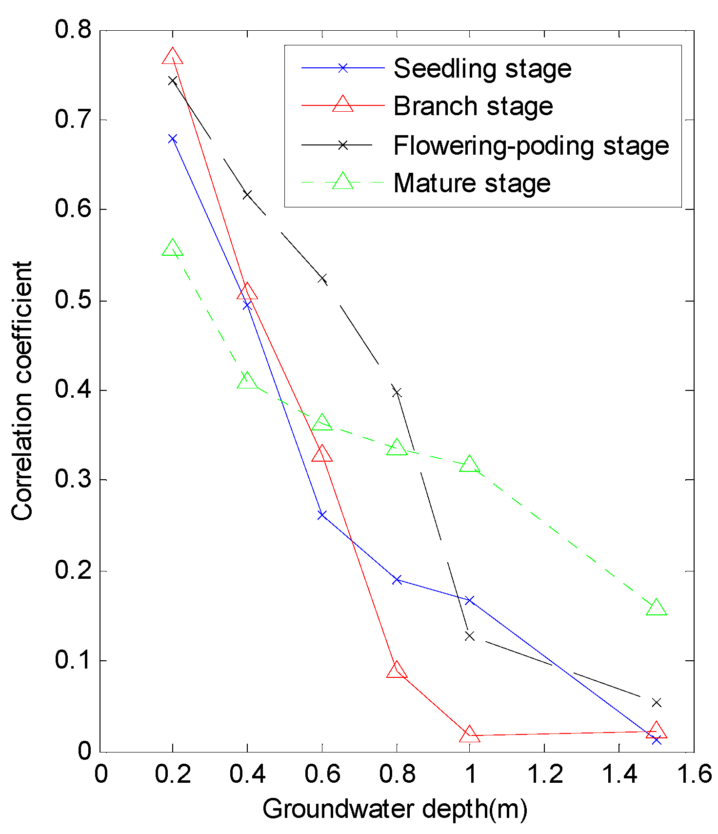
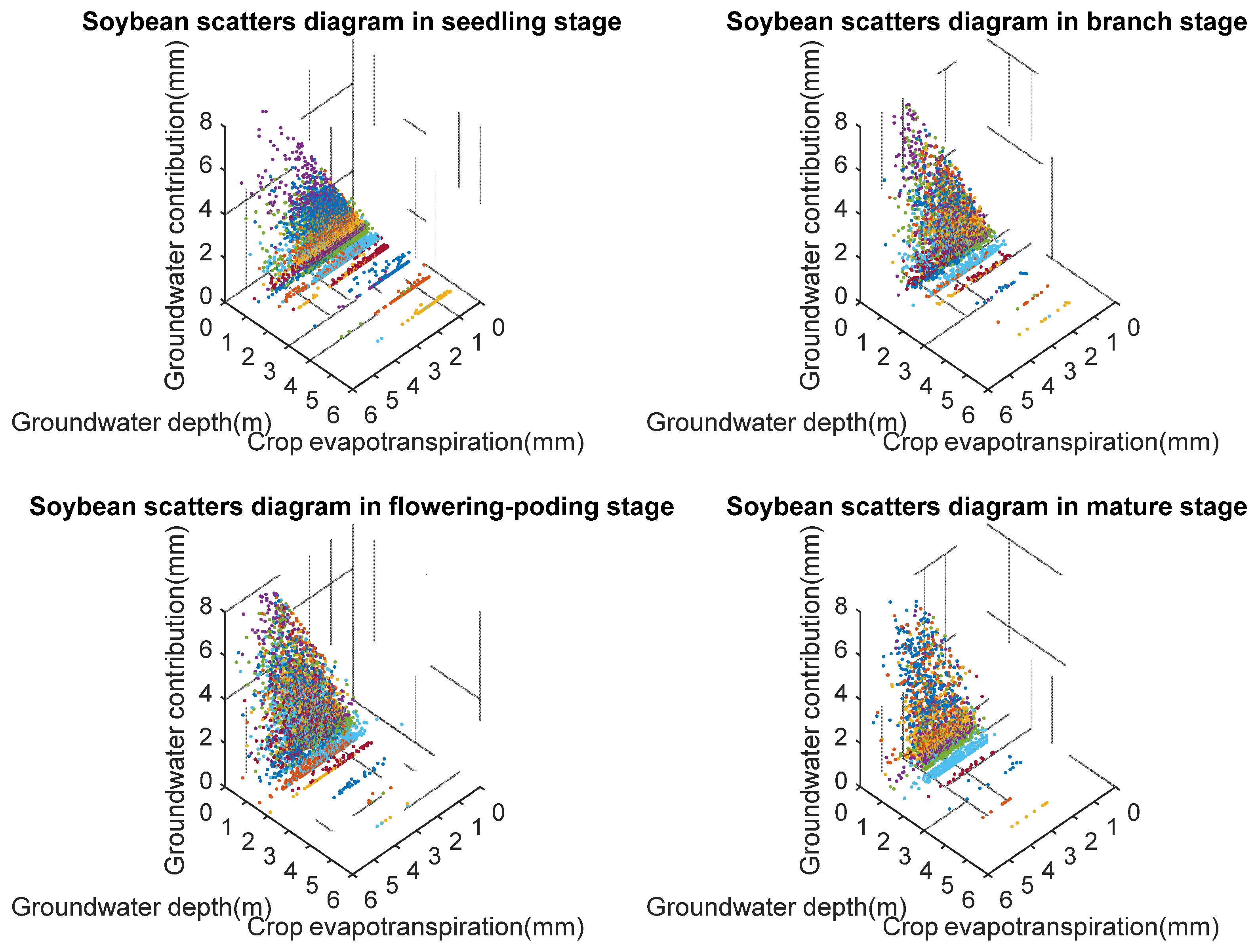
3.1. Relation Analysis between Groundwater Contribution and Soybean Evapotranspiration in the Different Soybean Growth Periods

Wind speed, relative humidity, and other atmospheric data were collected, and daily crop evapotranspiration from 1991 to 2005 was simulated using Equation (13). Soybean growth periods are shown in

Table 2. Detailed growth period times for soybeans.

Growth Periods of Soybean	Seedling Stage	Branch Stage	Flowering–Podding Stage	Mature Stage
Time	6.10–7.10	7.11–7.31	8.1–8.31	9.1–9.30

; for each soybean growth period from 1991 to 2005, two-dimensional scatter diagrams of soybean evapotranspiration and groundwater contribution at different groundwater depths were drawn. The diagrams for the flowering–podding stage are shown in Figure 4. For the different groundwater depths in each growth period, the correlation coefficients for groundwater contribution and soybean evapotranspiration were calculated, and the correlation coefficients of all growth periods are shown in Figure 5.

Figure 4 shows that the groundwater contribution increased with an increase in soybean evapotranspiration. The water in soybean evapotranspiration was due to the groundwater contribution, and the groundwater contribution affected soybean evapotranspiration. In addition, Figure 4 and Figure 5 show that with the increase in groundwater depth, the slope of the straight fit line gradually decreased, and the correlation coefficients of soybean evapotranspiration and groundwater contribution gradually decreased. The thick soil affected the movement of groundwater evaporation in the vertical vadose zone, and the degree of dependence between the groundwater contribution and soybean evapotranspiration gradually decreased. Since the linear relationship between groundwater use and crop evapotranspiration was not significant enough, we built nonlinear equations and models to fit the scatters of groundwater use and crop evapotranspiration.

The highest correlation coefficient in Figure 5 is 0.78, which is lower than 1. The water for soybean evapotranspiration was derived from soil water in the aeration zone, as well as from surface runoff, precipitation, and groundwater evaporation.

In terms of the relationship between the growth stages and the correlation coefficients between soybean evapotranspiration and shallow groundwater contribution, the correlation coefficients increased from the seedling to the branch and flowering–podding stages and decreased from the flowering–podding stage to the maturity stage. The variation in the correlation coefficient during the growth stages can be explained in combination with soybean growth characteristics. At the seedling stage, soybean roots are short [31] therefore, water from groundwater evaporation cannot be easily obtained, and the ratio of water from groundwater is low. As a result, the correlation coefficient was low. With the growth of the soybeans, the leaf area increased, and the water demand of soybeans increased in the branch and flowering–podding stages. The soybean roots became longer, and water was more easily obtained from groundwater. Therefore, the ratio of water from groundwater was larger, and the correlation coefficient between the groundwater contribution and soybean evapotranspiration was larger in the branch and flowering–podding stages. However, during the mature stage, soybean growth slowed, soybean water demand was low, and soybean evapotranspiration was primarily due to surface soil evaporation. As a result, the correlation coefficient between the groundwater contribution and soybean evapotranspiration was low in the mature stage.

The variation law of the correlation coefficient between shallow groundwater contribution and soybean evapotranspiration was different from that in deep groundwater. The main difference was that the correlation coefficient in the mature stage was larger than that in the flowering–podding stage in deep groundwater, whereas the correlation coefficient in the mature stage was smaller than that in the flowering–podding stage in shallow groundwater. This phenomenon is due to temperature. The seedling, branch, and flowering–podding stages occurred from June to August, there was no tendency for temperature variation, and there was no relationship between crop evapotranspiration and deep groundwater contribution. However, the mature stage occurred in September, and when the temperature gradually decreased, crop evapotranspiration also decreased. Meanwhile, the groundwater temperature at a depth of 1.5 m also decreased and the groundwater contribution decreased. As the variation trends of crop evapotranspiration and groundwater contribution were the same, the correlation coefficient between crop evapotranspiration and deep groundwater contribution was larger.

To show the variation trend in the groundwater contribution with an increase in soybean evapotranspiration and groundwater depth from a three-dimensional perspective, three-dimensional scatter diagrams were drawn (Figure 6). With increasing groundwater depth, soybean evapotranspiration and groundwater contribution decreased gradually. When the groundwater depth increased to 2.5 m, the groundwater contribution was approximately zero. Therefore, H_max in Equations (7)–(9) is equal to 2.5 m.

3.2. Error Comparison between the Machine Learning and Formula Methods

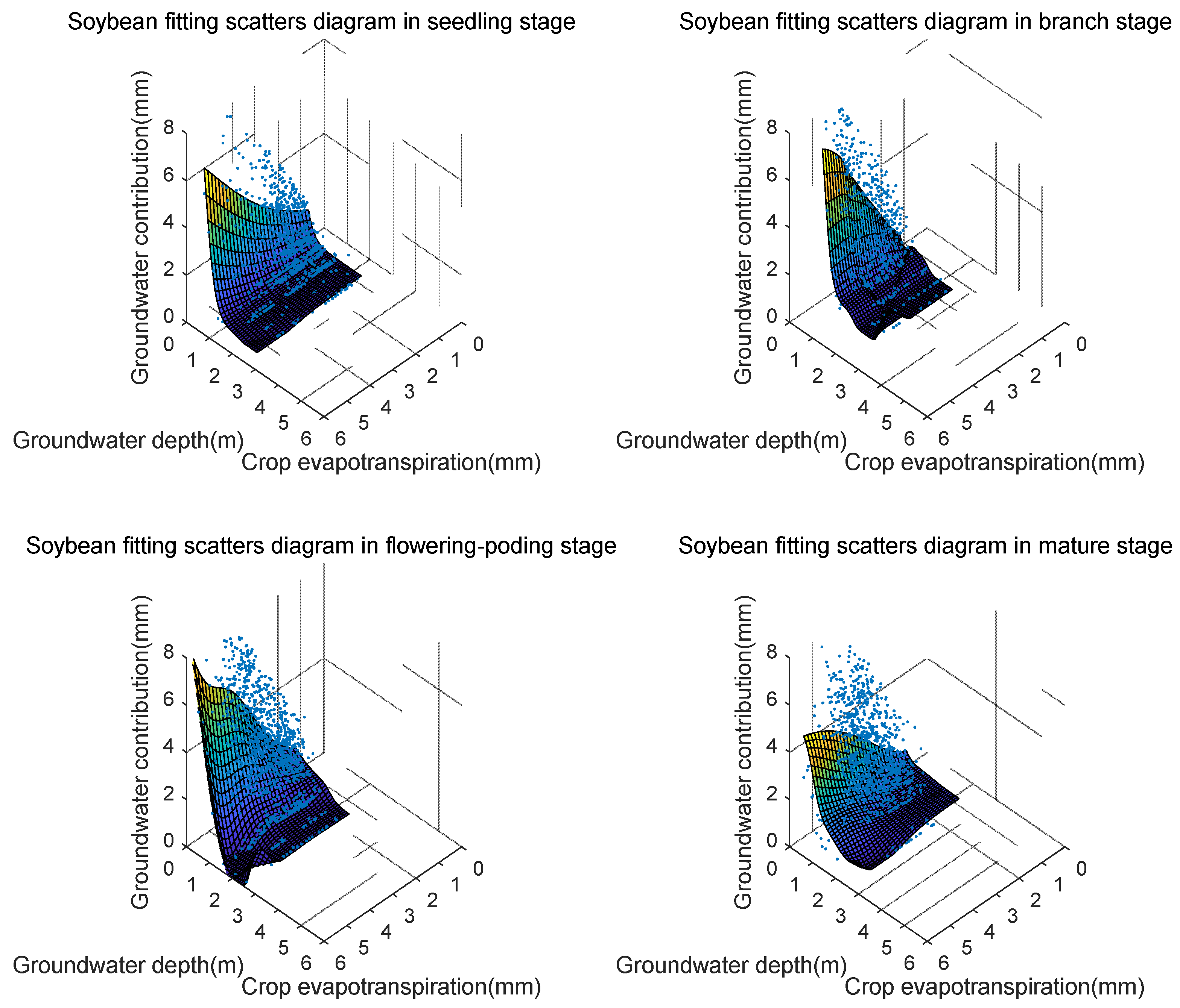
3.2.1. Fitting Errors

The scatter plots in Figure 6 were fitted using the machine learning and formula methods. In the machine learning method, soybean evapotranspiration and groundwater depth data from 1991 to 2002 were the inputs to the neural network, and groundwater contribution from 1991 to 2002 was the output of the neural network. The number of nodes and the total number of hidden layers were optimized using the GA, and the parameters of the weights and the bias in each layer were trained using the Levenberg–Marquardt algorithm. The fitting errors of the trained neural network are listed in

Table 3. Results and fitting errors of the machine learning and formula methods.

Methods	Parameters	Seedling Stage	Branch Stage	Flowering–Podding Stage	Mature Stage	Average
Machine learning	RME	0.788	1.133	1.107	1.324	1.088
	RMSPE	1.637	2.116	2.568	2.337	2.165
	R	0.836	0.806	0.771	0.634	0.762
Aviriyanover formula $$E_g=E{T}_c{\left(1-\frac{H}{H_{max}}\right)}^n$$	n	3.534	2.312	1.506	2.354	2.426
	RME	0.968	1.433	1.489	1.361	1.313
	RMSPE	1.675	2.592	3.018	2.429	2.429
	R	0.778	0.755	0.739	0.604	0.719
Ye Shuiting formula $$E_g=E{T}_c·{\mathrm{e}}^{-a_1\frac{H}{H_{max}}}$$	a1	4.052	2.725	1.908	2.854	2.884
	RME	0.984	1.599	1.748	1.450	1.445
	RMSPE	1.733	2.776	3.415	2.514	2.610
	R	0.775	0.755	0.736	0.612	0.719
Power function formula $$E_g=a·E{T}_c{\left(\frac{H}{H_{max}}\right)}^{-b}$$	a	0.041	0.115	0.221	0.166	0.136
	b	1.326	0.983	0.723	0.695	0.932
	RME	0.752	1.490	1.818	1.523	1.396
	RMSPE	1.514	2.675	3.617	2.594	2.600
	R	0.848	0.768	0.718	0.611	0.736

. In the formula method, combined with the data on groundwater depth, soybean evapotranspiration, and groundwater contribution from 1991 to 2002, the parameters of Equations (7)–(9) were optimized using an accelerated genetic algorithm (AGA) [26] and objective Function (5). The optimized parameters were fed into Equations (7)–(9), the simulated groundwater contribution was obtained using the three formulas, and the fitting errors were calculated based on Formulas (10)–(12).

The relative mean error (RME), root mean square percentage error (RMSPE), and correlation coefficient (R) ranks for the different methods are shown in

Table 4. Analysis of the assessment indices for machine learning and formula fitting.

Assessment Indices	Machine Learning	Aviriyanover Formula	Ye Shuiting Formula	Power Function Formula
RME	1.036	1.313	1.445	1.396
Rank of RME	1	2	4	3
RMSPE	2.092	2.429	2.61	2.6
Rank of RMSPE	1	2	4	3
R	0.763	0.719	0.719	0.736
Rank of R	1	3	3	2
Average rank	1	2.3	3.7	2.7

after comparing the statistical indices in Table 3.

From Table 4, it can be seen that the average rank of the error analysis was the best for machine learning, which indicates that its fitting effect was better than that of the formula method. Therefore, the machine learning method is recommended to fit the scatter of groundwater contribution, crop evapotranspiration, and groundwater depth.

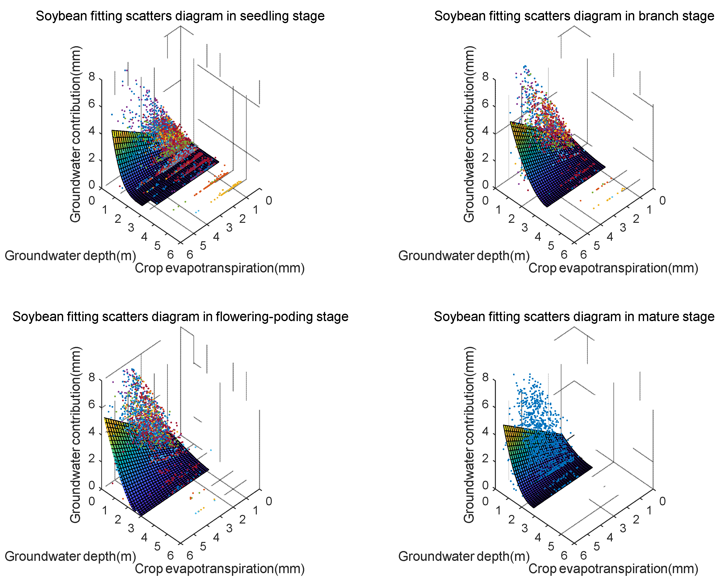
3.2.2. Validation Errors

In the last section, the groundwater contribution data from 1991 to 2002 were used to obtain the optimized formula methods and trained neural network method that were, in turn, used to calculate the groundwater contribution from 2004 to 2005. The validation errors for RME, RMSPE, and R are listed in

Table 5. Validation errors for groundwater contribution for the machine learning and formula methods.

Methods	Parameters	Seedling Stage	Branch Stage	Flowering–Podding Stage	Mature Stage	Average
Machine learning	RME	0.767	1.370	0.821	1.318	1.069
	RMSPE	1.582	2.902	1.817	2.241	2.136
	R	0.777	0.752	0.735	0.677	0.735
Aviriyanover formula $$E_g=E{T}_c{\left(1-\frac{H}{3}\right)}^n$$	RME	0.796	1.445	1.018	1.470	1.182
	RMSPE	1.472	2.860	2.467	2.639	2.360
	R	0.773	0.679	0.693	0.647	0.698
Ye Shuiting formula $$E_g=E{T}_c·{\mathrm{e}}^{-a_1\frac{H}{H_{max}}}$$	RME	0.852	1.482	1.096	1.518	1.237
	RMSPE	1.532	2.862	2.693	2.667	2.438
	R	0.768	0.680	0.686	0.651	0.696
Power function formula $$E_g=a·E{T}_c{\left(\frac{H}{H_{max}}\right)}^{-b}$$	RME	0.766	1.475	1.154	1.478	1.218
	RMSPE	1.524	3.057	2.758	2.548	2.472
	R	0.768	0.720	0.671	0.666	0.706

, combined with the observation data.

The ranks of the different methods with respect to RME, RMSPE, and R can be obtained in

Table 6. Analysis of the assessment indices for machine learning and formulae validation.

Assessment Indices	Machine Learning	Aviriyanover Formula	Ye Shuiting Formula	Power Function Formula
RME	1.036	1.182	1.237	1.218
Rank of RME	1	2	4	3
RMSPE	2.092	2.36	2.438	2.472
Rank of RMSPE	1	2	3	4
R	0.763	0.698	0.696	0.706
Rank of R	1	3	4	2
Average rank	1	2.3	3.7	3

after comparing the statistical indices in Table 5.

Table 6 shows that the average rank of the error indices for the machine learning method is excellent at 1; and the Aviriyanover, power function, and Ye Shuiting formulae had lower ranks of error analysis. Because of its high precision, the machine learning method is recommended to further calculate groundwater contribution.

Based on Figure 6, three-dimensional diagrams of the fitting scatter were drawn using the machine learning method.

In Figure 7, the variation trend can be observed from an overall three-dimensional perspective. Figure 7 shows that with an increase in soybean evapotranspiration and a decrease in groundwater depth, the groundwater contribution increases gradually. The fitted curved surface is inclined toward the positive direction of the axis of groundwater contribution. To compare the fitted curved surfaces, fitting scatter diagrams for soybeans using the Aviriyanover formula are shown in Figure 8. There is a similar trend between fitting the curved surface using machine learning and the Aviriyanover formula method. However, the surface in Figure 8 is smoother than that in Figure 7 because there are more parameters in the neural network of Figure 7. The neural network, with five nodes of one hidden layer, has 21 parameters, including 15 weight values and six bias values, whereas the Aviriyanover formula has only one parameter. Owing to its additional parameters, the machine learning method can be adjusted to better fit the scatter, as shown in Figure 7. Therefore, the precision of the machine learning method is better than that of the formula methods.

Figure 7 and Figure 8 show that the groundwater depth gradually deepened at the same soybean evapotranspiration and groundwater contribution from the seedling to the branch- and flowering-poding stages, but it became shallower from the flowering–podding stage to the mature stage. The soybean roots at the seedling stage were short, and the groundwater contribution was mainly from shallow groundwater. Subsequently, in the middle of the growth period, the soybeans grew vigorously, their roots were long, and they could access deeper groundwater. Therefore, with an increase in groundwater depth and a decrease in soybean evapotranspiration, the groundwater contribution decreased slowly. However, in the mature stage, the soybeans grew slowly, and although the roots were long, the water demand decreased, which contributed to an abrupt decrease in groundwater contribution, with an increase in groundwater depth and a decrease in soybean evapotranspiration. The fitting surface is relevant to the weights and biases of the neural network method, which indicates that the parameters of the neural network method are linked to growth characteristics and groundwater contribution.

4. Conclusions

The main goal of the current study was to improve the modeling of groundwater contribution and to compare groundwater contribution calculation methods, including machine learning and the formula methods of Aviriyanover, Ye Shuiting, and the power function. Data relating to groundwater depth, groundwater contribution, and atmospheric data from 1991 to 2005 were collected from a test station in Xinmaqiao, China, and the relationship between groundwater contribution and soybean evapotranspiration in different growth stages was analyzed. The errors and fitting surface characteristics of the trained neural network method and formula methods based on AGA were also analyzed. The conclusions are as follows.

(1)

As part of soybean evapotranspiration, the groundwater contribution increased with an increase in soybean evapotranspiration. In addition, the correlation coefficients of soybean evapotranspiration and groundwater contribution gradually decreased with increasing groundwater depth because of the influence of thick soil layers on the movement of groundwater evaporation in the vertical vadose zone.

(2)

The correlation coefficients between groundwater contribution and soybean evapotranspiration increased from the seedling to the branch and flowering–podding stages and decreased from the flowering–podding stage to the maturity stage. The short roots of soybeans at the seedling stage led to a low correlation coefficient of 0.68. The longer roots and larger leaf area of soybeans at the branch and flowering–podding stages led to high correlation coefficients of 0.78 and 0.75, respectively. Low soybean water demand caused a low correlation coefficient of 0.57 in the mature stage.

(3)

Through this study, we found that machine learning had the best performance for fitting errors, with values for relative mean error (RME), root mean square percentage error (RMSPE), and correlation coefficient of 1.088, 2.165, and 0.762, respectively; in addition, for validation errors, we observed values for RME, RMSPE, and correlation coefficient of 1.069, 2.136, and 0.735, respectively, compared with those of the formula method, which can be explained by more parameters in the neural network. The fitting surface of the formula method is smoother than that of the machine learning method due to the existence of more parameters in the neural network. The machine learning method is recommended for readers seeking to calculate the groundwater contribution.

The recommended machine learning method can be used in hydrological and crop growth models. Many hydrological models do not consider the influence of the groundwater contribution on the water balance equation and the water cycle. The machine learning method can be added to the groundwater module of hydrological models, and groundwater contribution should be added to the water balance equation for groundwater. In addition, machine learning methods can be used in crop growth models, and there may be greater crop transpiration.

References

1. Yang, X. Research progress on the utilization of shallow groundwater under the planting conditions of crops. J. Anhui Agric. Sci. 2008, 36, 9650–9651+9673. (In Chinese) [Google Scholar]
2. Zhu, M.; Ahmed, B.N.; Li, X.L.; Huang, M.N.; Muhammad, T.; Ming, L. Shallow groundwater utilization role of wheat based on different soil and different groundwater depth. Fresen. Environ. Bull. 2018, 27, 3495–3505. [Google Scholar]
3. Zhao, Y.; Li, F.W.; Wang, Y.; Jiang, R.G. Evaluating the effect of groundwater table on summer maize growth using the AquaCrop model. Environ. Model. Assess. 2020, 25, 343–353. [Google Scholar] [CrossRef]
4. Wang, X.; Hou, H. Study on shallow groundwater evaporation laws of crops and bare soil. J. Hydroelectric. Eng. 2008, 27, 60–65. (In Chinese) [Google Scholar]
5. Costelloe, J.F.; Irvine, E.C.; Western, A.W. Uncertainties around modelling of steady-state phreatic evaporation with field soil profiles of δ18O and chloride. J. Hydrol. 2014, 511, 229–241. [Google Scholar] [CrossRef]
6. Aviriyanover, C.Φ. The Level Drainage Facilities to Control the Irrigation Salinizatio; China Industry Press: Beijing, China, 1985. (In Chinese) [Google Scholar]
7. Ye, S.; Shi, X.; Miao, X. Analysis of hydration degree problem with phreatic evaporation empirical formula. Hydrogeol. Eng. Geol. 1982, 45–48+6. (In Chinese) [Google Scholar]
8. Hu, S.; Kang, S.; Song, Y.; Tian, C.; Pan, Y.; Li, Y. Variation of phreatic evaporation and its calculation method in Tarim River Basin in Xinjiang Region. Trans. Chin. Soc. Agric. Eng. 2004, 49–53. (In Chinese) [Google Scholar]
9. Zhidong, L.; Shixiu, Y.; Senchuan, X. Soil Water Dynamics; Tsinghua University Press: Beijing, China, 1988. (In Chinese) [Google Scholar]
10. Fidantemiz, Y.F.; Jia, X.; Daigh, A.; Hatterman-Valenti, H.; Steele, D.; Rashid Niaghi, A.; Simsek, H. Effect of water table depth on soybean water use, growth, and yield parameters. Water 2019, 11, 931. [Google Scholar] [CrossRef] [Green Version]
11. Zhou, C.; Wang, Z. Experiment on phreatic evaporation of bare soil and soil with crop in the field of Shajiang black soil. Anhui Agric. Sci. Bull. 2018, 24, 81–83. (In Chinese) [Google Scholar]
12. Wang, Z.; Yang, M.; Lv, H.; Hu, Y.; Zhu, Y.; Gu, N.; Wang, Y. Phreatic evaporation in bare and wheat land during freezing-thawing period of Huaibei Plain based on lysimeters experiments. Trans. Chin. Soc. Agric. Eng. 2019, 35, 129–137. (In Chinese) [Google Scholar]
13. Karimov, A.K.; Šimůnek, J.; Hanjra, M.A.; Avliyakulov, M.; Forkutsa, I. Effects of the shallow water table on water use of winter wheat and ecosystem health: Implications for unlocking the potential of groundwater in the Fergana Valley (Central Asia). Agric. Water Manag. 2014, 131, 57–69. [Google Scholar] [CrossRef]
14. Shah, N.; Nachabe, M.; Ross, M. Extinction depth and evapotranspiration from ground water under selected land covers. Groundwater 2007, 45, 329–338. [Google Scholar] [CrossRef] [PubMed]
15. Sreekanth, P.D.; Geethanjali, N.; Sreedevi, P.D.; Ahmed, S.; Kumar, N.R.; Jayanthi, P.D.K. Forecasting groundwater level using artificial neural networks. Curr. Sci. 2009, 96, 933–939. [Google Scholar]
16. Daliakopoulos, I.N.; Coulibaly, P.; Tsanis, I.K. Groundwater level forecasting using artificial neural networks. J. Hydrol. 2005, 309, 229–240. [Google Scholar] [CrossRef]
17. Rakhshandehroo, G.R.; Vaghefi, M.; Aghbolaghi, M.A. Forecasting Groundwater Level in Shiraz Plain Using Artificial Neural Networks. Arab. J. Sci. Eng. 2012, 37, 1871–1883. [Google Scholar] [CrossRef]
18. Mohammadi, K. Groundwater Table Estimation Using MODFLOW and Artificial Neural Networks. In Proceedings of the General Assembly of the European-Union-of-Geosciences, Vienna, Austria, 24–29 April 2005; pp. 127–138. [Google Scholar]
19. Zhu, C.J.; Xie, H.H.; Huang, X.K. Evaluation of groundwater quality using Artificial Neural Network. In Proceedings of the International Symposium on Knowledge Acquisition and Modeling, Wuhan, China, 21–22 December 2008; pp. 158–160. [Google Scholar]
20. Zhu, C.J.; Hao, Z.C.; Ju, Q.; Ieee. A prediction of groundwater quality using Grey System Neural Network United Model. In Proceedings of the 21st Chinese Control and Decision Conference, Guilin, China, 17–19 June 2009; pp. 3216–3219. [Google Scholar]
21. Sunayana; Kalawapudi, K.; Dube, O.; Sharma, R. Use of neural networks and spatial interpolation to predict groundwater quality. Env. Dev. Sustain 2020, 22, 2801–2816. [Google Scholar] [CrossRef]
22. Kulisz, M.; Kujawska, J.; Przysucha, B.; Cel, W. Forecasting water quality index in groundwater using Artificial Neural Network. Energies 2021, 14, 5875. [Google Scholar] [CrossRef]
23. Demuth, H.B.; Beale, M.H.; Jess, O.D.; Hagan, M.T. Neural Network Design; Martin Hagan: Stillwater, OK, USA, 2014. [Google Scholar]
24. Hagan, M.T.; Menhaj, M.B. Training feedforward networks with the Marquardt algorithm. IEEE Trans. Neural Netw. 1994, 5, 989–993. [Google Scholar] [CrossRef]
25. Wang, Z.; Liu, M.; Li, R. Experiment on phreatic evaporation of bare soil and soil with crop in Huaibei plain. Trans. Chin. Soc. Agric. Eng. 2009, 25, 26–32. (In Chinese) [Google Scholar]
26. Jin, J.; Yang, X.; Ding, J. An improved simple genetic algorithm - accelerating genetic algorithm. Syst. Eng. Theory Pract. 2001, 21, 8–13. (In Chinese) [Google Scholar]
27. Bi, J. Macroeconometric Model in China: Structural Analysis, Policy Simulation, and Economic Forecasting; Peking University Press: Beijing, China, 1994; p. 234. (In Chinese) [Google Scholar]
28. Luo, Y.; Mao, Y.; Peng, S.; Zhen, Q.; Wang, W. Modified Aver’yanov’s phreatic evaporation equations under crop growing. Trans. Chin. Soc. Agric. Eng. 2013, 29, 102–109. (In Chinese) [Google Scholar]
29. Allen, R.; Pereira, L.; Raes, D.; Smith, M. Crop evapotranspiration guidelines for computing crop water requirements. FAO Irrig. Drain. Pap. 1998, 300, 24. [Google Scholar]
30. Zhao, Y.; Wang, Y.; Duo, Y. Discussion on some issues of crop evapotranspiration. South--North. Water. Transfers. Water Sci. Technol. 2005, 3, 57–59. (In Chinese) [Google Scholar]
31. Luo, Y.; He, C.; Sophocleous, M.; Yin, Z.; Hongrui, R.; Ouyang, Z. Assessment of crop growth and soil water modules in SWAT2000 using extensive field experiment data in an irrigation district of the Yellow River Basin. J. Hydrol. 2008, 352, 139–156. [Google Scholar] [CrossRef]
Figure 1. The schematic diagram of the Mariotte bottle system for observing the groundwater contribution of soybeans.
Water 14 03092 g001
Figure 2. The structure of the neural network.
Water 14 03092 g002
Figure 3. The location of the test station.
Water 14 03092 g003
Figure 4. Scatter diagrams of soybean evapotranspiration and groundwater contribution for various groundwater depths in the flowering–podding stage.
Water 14 03092 g004
Figure 5. Changes in the correlation coefficient considering the amount of soybean evapotranspiration and groundwater contribution along with depth in different growth stages.
Water 14 03092 g005
Figure 6. Three-dimensional scatter diagrams of groundwater depth, crop evapotranspiration, and the groundwater contribution of soybean in different growth periods.
Water 14 03092 g006
Figure 7. Fitting scatter diagrams for groundwater depth, crop evapotranspiration, and groundwater contribution in each growth period for soybeans using the machine learning method.
Water 14 03092 g007
Figure 8. Fitting scatter diagrams for groundwater depth, crop evapotranspiration, and groundwater contribution in each growth period for soybeans using the Aviriyanover formula method.
Water 14 03092 g008