
Simulation Analysis of the Cooling Effect of Urban Water Bodies on the Local Thermal Environment


School of Geomatics and Urban Spatial Information, Beijing University of Civil Engineering and Architecture, Beijing 102616, China
*
Author to whom correspondence should be addressed.
Water 2022, 14(19), 3091; https://doi.org/10.3390/w14193091
Submission received: 2 August 2022
/
Revised: 23 September 2022
/
Accepted: 26 September 2022
/
Published: 1 October 2022
(This article belongs to the Section Urban Water Management)
Abstract
:Urban water bodies have a cooling effect and alter the local urban thermal environment. However, current research is unclear regarding the relationships between factors such as the spatial density, area proportion, and distribution pattern of water bodies and the cooling effect of water on the local thermal environment. To clarify these relationships, it is critical to quantify and evaluate the influence these factors have on the cooling effect of water in the urban landscape. Therefore, we analyzed the cooling effect of different water bodies on the local thermal environment at the microscale by comparing their area proportions and distribution patterns using numerical simulations. Furthermore, we analyzed the day–night variation in the cooling effect of urban water bodies with different areas and distribution patterns. We used the area proportion, separation index (SI), and landscape shape index (LSI) to indicate the layouts of water bodies. The results showed that the cooling effect of a water body was higher during the day than at night. These results also showed that area proportion and LSI were positively correlated with the water body’s cooling effect. However, the efficiency of the cooling effect gradually decreased with increasing area proportion. When the LSI increased, more areas within the region displayed larger cooling effect values, but the uniformity of the regional cooling diminished. Additional results showed that the cooling effect had no significant positive correlation with SI. A moderate SI could enhance the uniformity of the cooling effect in the region and link the cooling effect between water patches.
1. Introduction
With accelerating urbanization, the urban-scale heat island effect becomes more pronounced. Under the urban heat island (UHI) effect, urban spaces do not form high-temperature isothermal regions but present isolated centers of high temperature. UHIs not only affect people’s living environment and quality of life but also can cause serious harm to the urban ecosystem and public safety, affect the urban material cycle and energy flow, and aggravate air pollution, thus affecting the development of cities.
In recent years, various mitigation efforts or acts of governance have been undertaken to reduce the impact of UHIs. Using green and blue infrastructure to reduce the temperature of the surrounding urban environment is one of the most effective ways to mitigate the urban heat environment [1,2,3,4,5]. Urban blue infrastructure consists of water bodies in urban landscapes. Various water bodies in urban landscapes offer significant potential value in regulating the urban microclimate and reducing urban air temperatures [6]. Many studies showed that water bodies have a significant cooling effect [7,8,9]. Water bodies have high thermal inertia, heat capacity, and thermal conductivity, and low emissivity [10]. Because water has only one surface with which to absorb solar radiation, the ability of urban water bodies to absorb heat is weaker than that of buildings. Therefore, according to the theory of surface heat balance, water bodies not only correspond to relatively low surface temperatures but also influence the ambient temperature of the surrounding environment.
Many factors affect water bodies’ cooling effect, including factors specific to each water body and local environmental factors. The ability of water bodies to regulate the local microclimate can be realized by planning the area, shape and spatial heterogeneity of different water bodies [11]. In terms of water body area, the proportion of water surface is significantly negatively correlated (correlation coefficient of −0.72) with the surface temperature of the water body [12]. The larger the area of the water body, the more heat radiation it absorbs, and the larger its evaporation area. The larger the area of evaporation, the more heat in the air is dissipated through evaporation, and the lower the resulting air temperature and radiation temperature values [13]. The water body’s patch area is the dominant cooling intensity factor [14]. However, in reality, the area of water bodies is limited. Therefore, water bodies’ shape and spatial heterogeneity can also be designed to maintain their maximum value for microclimate regulation. The shape and spatial heterogeneity of water bodies can be quantified by applying a landscape index [15]. The cooling effect of water decreases nonlinearly as the distance from the water body increases [16]. The shape of a body of water is usually represented by the landscape shape index (LSI). The smaller LSI of the water body is, the greater the UHI effect is [17]. The LSI of the water body has a high correlation with the cooling effect of the water body [18,19,20]. In terms of spatial heterogeneity, numerous smaller water bodies can provide more beneficial cooling effects than fewer large water bodies with the same total area [21]. In addition, widely distributed, discrete water bodies have a better cooling effect than concentrated water bodies [22,23]. Therefore, parametric indicators are necessary to quantitatively study the cooling effects of different water bodies.
To quantify the cooling effect of water bodies, three methods are commonly used: field measurement [24,25,26], monitoring by remote sensing [20,27,28], and microscopic simulation [29,30,31]. Although field measurements are accurate, the cost of observation is high, and the scale is limited. Remote sensing methods primarily focus on the relationship between the cooling effect’s intensity and range and the areas and spatial patterns of water bodies. Remote sensing methods tend to analyze the annual seasonal variation or long-term interannual variation in the cooling effect of water bodies. Compared with field measurement, microscopic simulation does not require much manpower or time. Compared with remote sensing, microscopic simulation has the advantages of resolution and dimension and can obtain 3-D temperature data at the meter scale. The computational fluid dynamics (CFD) model is one of the important microscopic simulation methods. ENVI-met is the most widely used software for analyzing the influence of different underlying surfaces on urban microclimate. For example, ENVI-met was used to simulate the layout factors of water bodies, and a microscale model was constructed to simulate the water bodies’ scale, dispersion, morphology, and location. The cooling effects under different water body configurations were simulated, and the water body configuration with the best cooling effect was determined [22].
Based on previous studies, we found it very important to quantify the cooling effect of urban water bodies. However, at present, most studies on the cooling effect of water bodies start from remote sensing monitoring to analyze the cooling effect of water bodies, especially of large rivers and lakes. There are few quantitative studies on the cooling effect of artificial rivers, pools, and other landscape water bodies in urbanized areas seriously affected by human activities at the microscale, and the factors affecting the cooling effect. Therefore, we took urban artificial water bodies as an example and used numerical simulation to analyze the cooling effect of water bodies quantitatively. The specific objectives of this study were as follows: (1) to determine the effect of different area proportions of water bodies on the cooling effect of urban water bodies; (2) to use different layout indices to quantify the layout of water bodies; (3) to determine the influence of different water body distribution patterns on the cooling effect of urban water bodies.
2. Method
We used the urban microclimate simulation software ENVI-met for the simulation experiments. ENVI-met software is based on relevant theoretical knowledge, such as thermodynamics, computational fluid dynamics, and urban ecology. It fully considers the interactions between the ground, vegetation, architecture, and atmosphere in small-scale urban spaces and can numerically simulate and reproduce the dynamic urban atmospheric change process. The numerical simulation of dynamic urban atmospheric change incorporates air flow, turbulence, heat and water exchange between plants and the surrounding environment, particle diffusion, and heat and water vapor exchange on the ground and building surfaces. Therefore, ENVI-met software is essential for studying the urban heat island effect, building natural ventilation, and exploring atmospheric pollutant diffusion [32].
2.1. Boundary Condition of Simulation
As an example, we studied the cooling effect of urban water landscapes on the urban microclimate in the Beijing area. The simulation area was 100 m × 100 m, located at 116.4° E and 39.91° N. According to the characteristics of the ENVI-met numerical simulation, the grid was set to 100 × 100 × 30. The grid resolution was dx = 1 m, dy = 1 m, and dz = 2 m (dx and dy are the horizontal resolutions of the X and Y axes, respectively, and dz is the vertical resolution of the Z axis). 31 July 2018, was selected as the simulation day, and the simulation time was 24 h from 0:00. Based on the day’s meteorological data from Beijing, the initial wind speed was set to 1.8 m/s, the dominant wind direction was 180°, the initial temperature was 30 °C, and the relative humidity was 72%.
2.2. Simulation Design
2.2.1. Simulation of Different Water Body Area Proportions
To ensure that the surrounding environment remained unchanged, we used the control variable method to set up a green space with a coverage rate of 30% around the water body. With the shape and layout of the water body unchanged, we set up eight different models of the area proportion of water bodies, with water body area proportions of 0%, 1%, 4%, 9%, 16%, 25%, 36%, 49%, and 64%, referring to the ratio of the area of water bodies to the area of the surrounding region. The water body area proportion refers to the proportion of water body area to the area of the area where it is located, and is calculated as follows:
where is the area proportion of the water bodies, is the total simulation area, and is the total area of water patches.
The models of the area proportion for each water body constructed by ENVI-met software are shown in Table 1, where the surfaces other than the water body were set as bare soil.
2.2.2. Simulation of Different Water Body Layouts
The spatial heterogeneity and shape of the water bodies are important factors for water body layout. To describe the simulation results, we used two quantitative indices to quantify the differences between different layouts. We used the Separation Index (SI) to denote the water bodies’ spatial heterogeneity [33]; it was calculated as follows:
where is the minimum boundary distance from each patch to the nearest neighbor patch, is the number of water patches, is the total area of water patches. SI describes the degree of dispersion of the water bodies. A larger SI indicates that the more distant the patches are from each other, the more discrete the distribution of patches.
We used Landscape Shape Index (LSI) to denote the water bodies’ shape. LSI is a shape index of water body patches, a standardized measure of total edge or margin density that can be adjusted to the size of the landscape [34]; it was calculated as follows:
where is the perimeter of a single water patch, is the area of a single water patch. LSI illustrates the complexity of the shape of the water body. Ideally, the LSI equals 1.00 for a circle and 1.13 for a square. It increases with increasing landscape shape irregularity. A larger LSI indicates a more irregular shape, leading to a larger contact surface between the water body and the surrounding environment.
We selected a water body with an area proportion of 16%, established six layout models, and simulated the above indicators with the layout elements shown in Table 2. The effects of SI on the cooling effect of water bodies are discussed using cases 1, 2, 3, and 4. The effects of LSI on the cooling effect of water bodies are discussed using cases 1, 6, and 7.
3. Results
3.1. The Effect of Area Proportion on the Cooling Effect
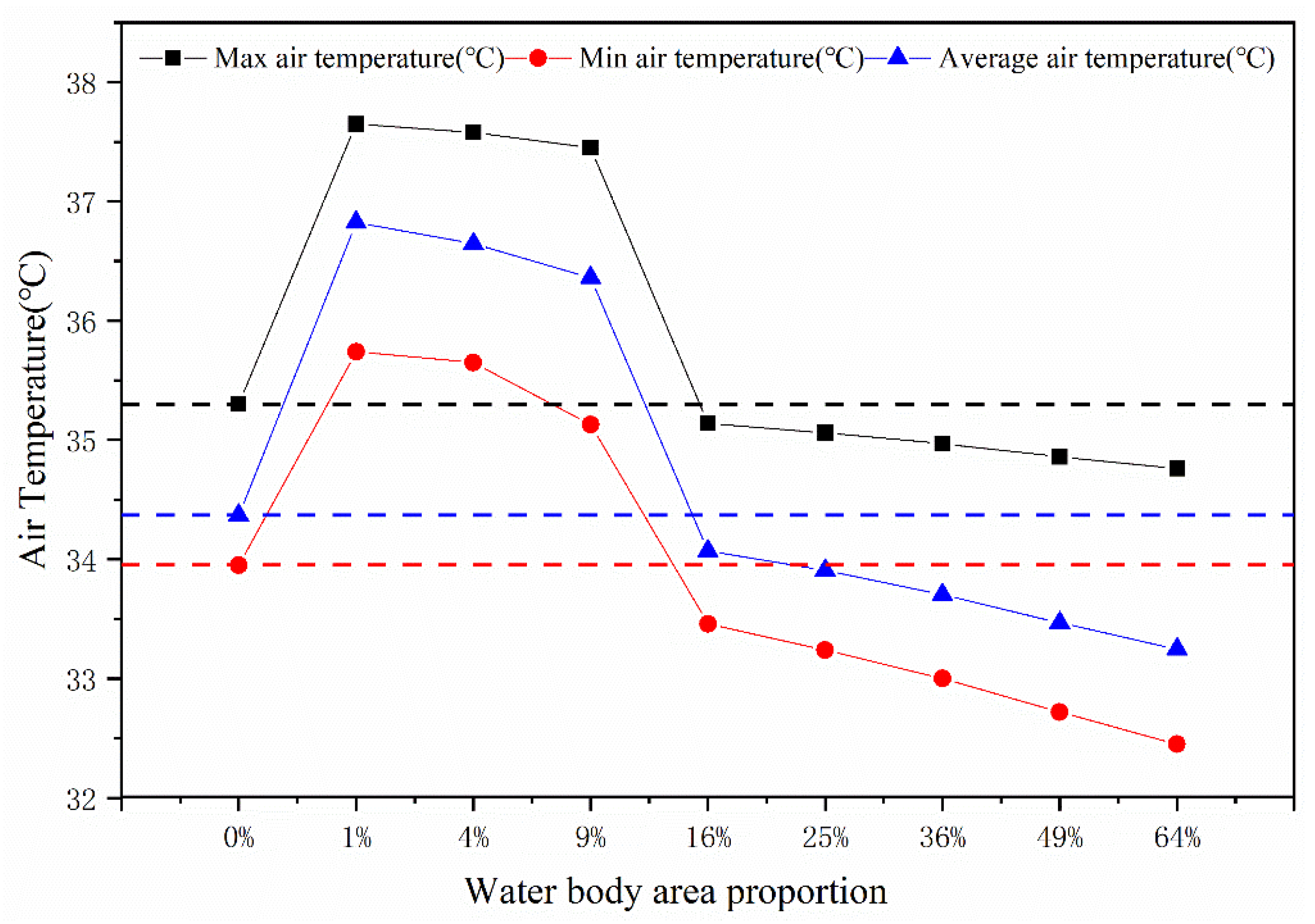
We analyzed the maximum, minimum, and average temperatures of water bodies with different area proportions at 14:00. From Figure 1, we can see that the temperature gradually decreased as the area proportion of the water body increased. However, when comparing with the air temperature at 14:00 for water bodies with a 0% area proportion, water bodies with 1%, 4%, and 9% area proportions did not have a cooling effect on the surrounding environment, and even increased the air temperature. Therefore, we analyzed the experimental results for the effects of water body area proportions of 16%, 25%, 36%, 49%, and 64% on the cooling effect.
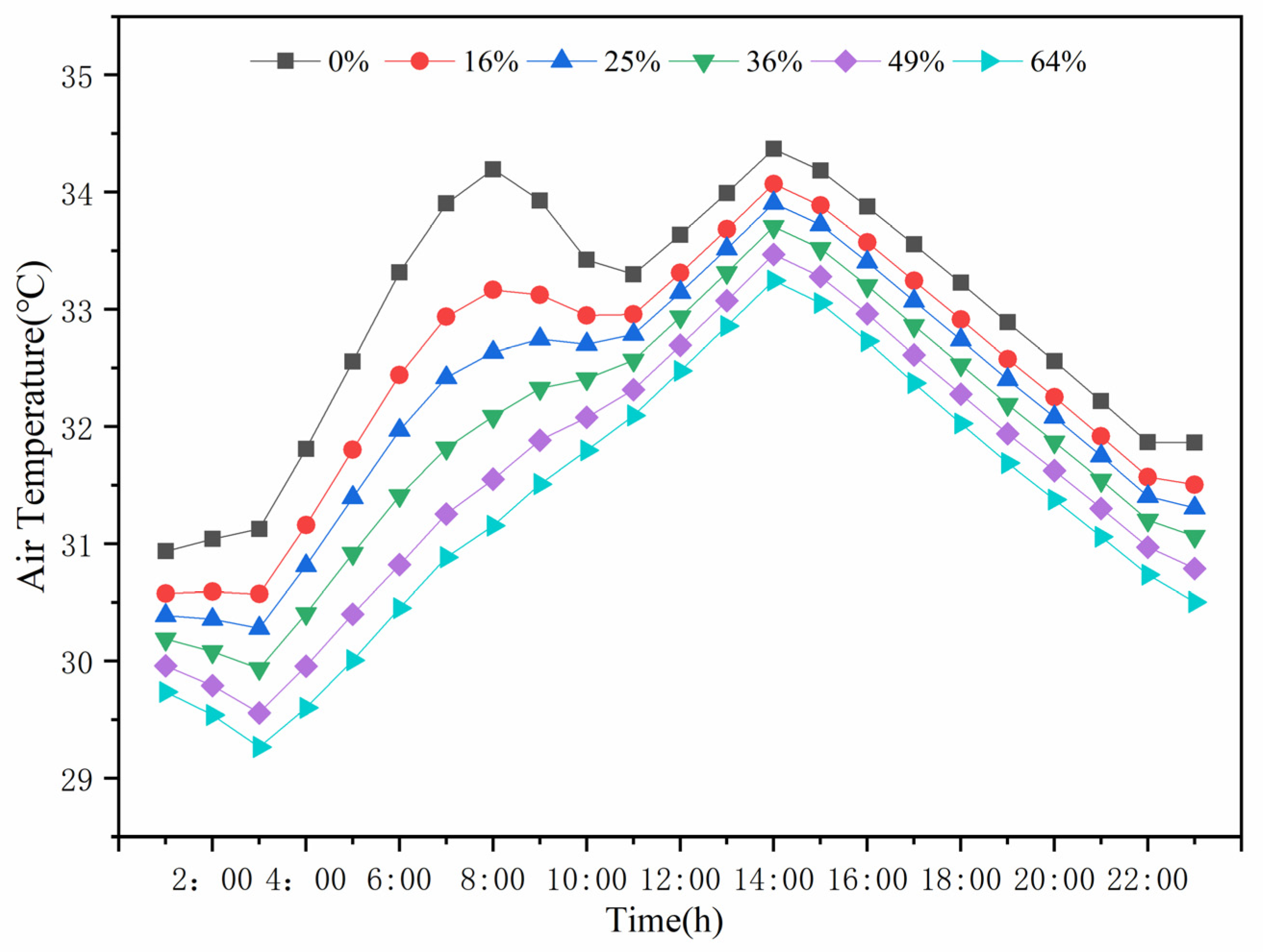
The hourly temperature changes throughout the day under each water body area proportion are shown in Figure 2. The daily minimum temperature occurred at 3:00, and the daily maximum temperature occurred at 14:00. The water bodies with area proportions of 0%, 16%, and 25% had brief temperature drops at 8:00. The temperature started to increase at 10:00 and reached a maximum at 14:00. For water bodies with area proportions of 36%, 49%, and 64%, the temperature began to increase gradually after 3:00 and reached its highest value at 14:00.
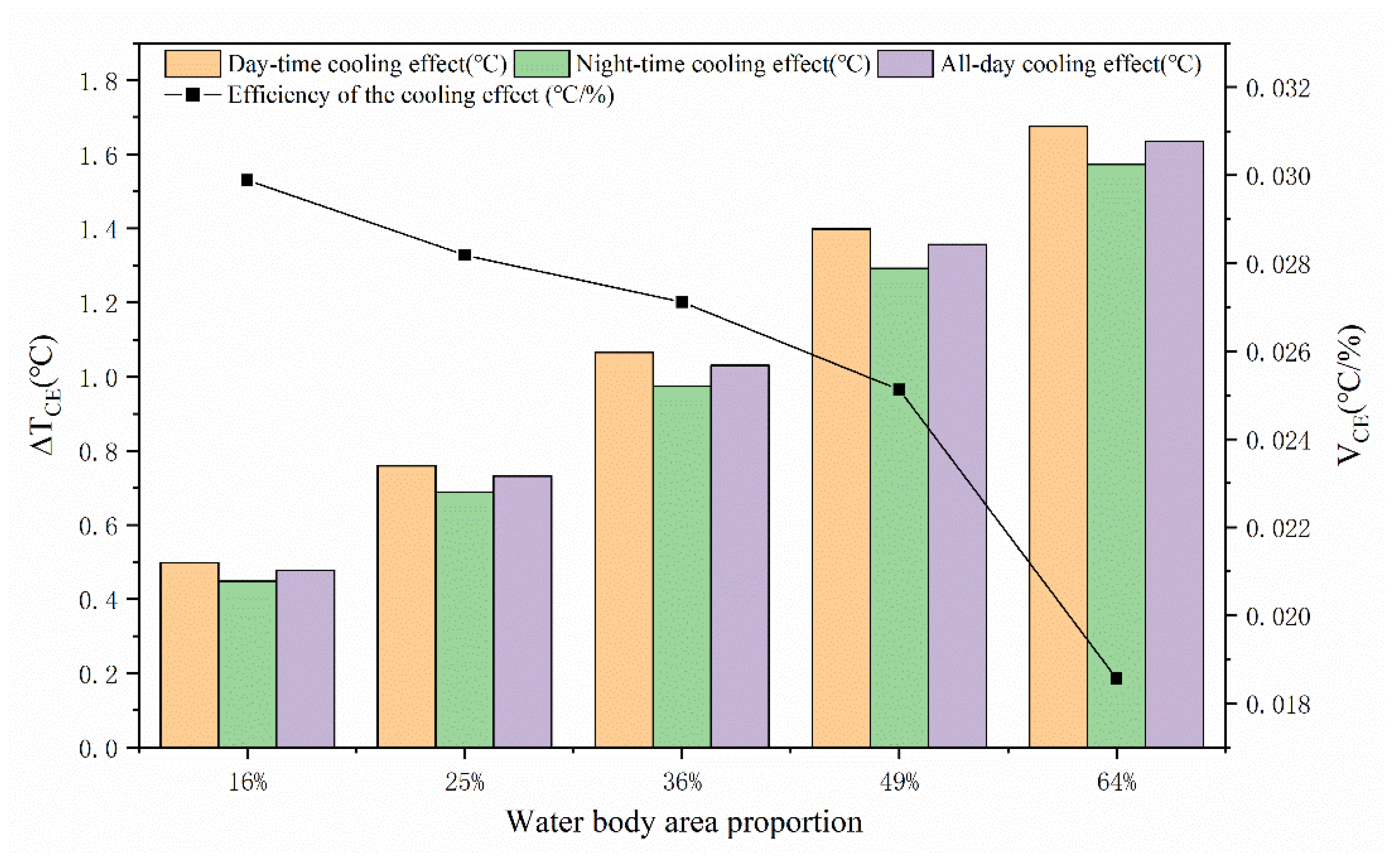
Based on the sunrise and sunset times on 31 July 2018, we used the period of 6:00–19:00 as the daytime and the rest of the period as the nighttime. The daytime, nighttime, and all-day cooling effects for each selected water body area proportion are shown in the histogram in Figure 3. The cooling effect is denoted by , and is calculated as follows:
where is the average temperature in the scenario with the water body, is the average temperature in the scenario without the water body, and the unit of is °C.
We expressed the speed of enhancement of the all-day cooling effect for each water body area proportion with respect to the previous area proportion in terms of the efficiency of cooling effect enhancement, as shown in the line graph in Figure 3. We used to denote the efficiency of cooling effect enhancement; it is calculated as follows:
where is the water body area proportion and is the area proportion of the previous water body (i.e., the previous ). and are the cooling effects under their respective area proportion scenarios. The unit of is °C/%.
Figure 3 shows that the water body cooling effect increased as the area proportion of the water body increased. In the case of identical water body area proportions, the cooling effect of the water body was more significant during the day than at night. With increases in the area proportion of the water body, the efficiency of the water body cooling showed a decreasing trend. When the area proportion of the water body was 16%, was 0.030 °C/%; when the area proportion of the water body was 64%, was 0.019 °C/%.
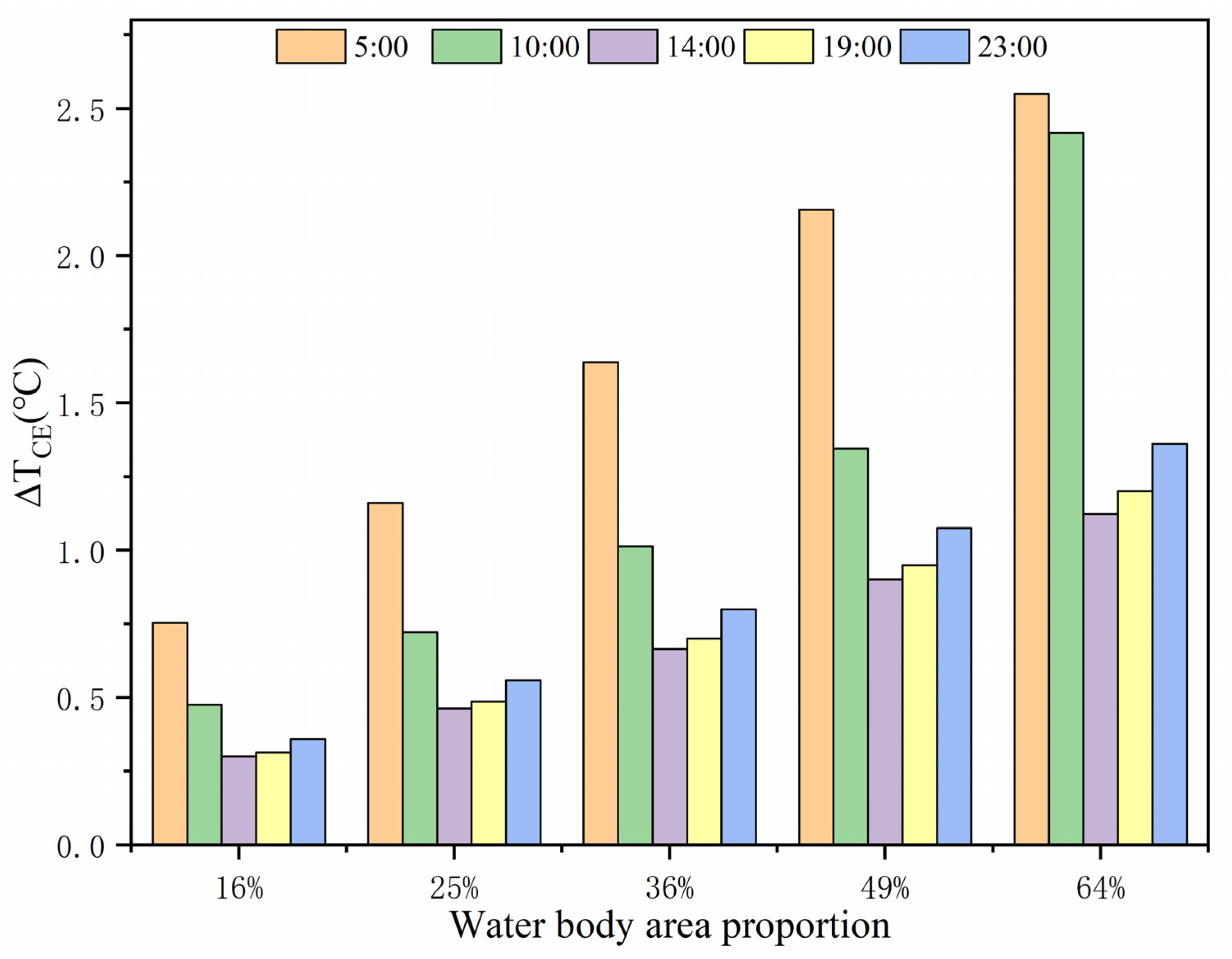
We selected five typical times of the day, 5:00, 10:00, 14:00, 19:00, and 23:00, to simplify the daily temperature changes. 5:00 and 19:00 were the times of sunrise and sunset, respectively. 10:00 was in the sunrise temperature rise stage, 14:00 was in the highest temperature stage of the day, and 23:00 was the time when the temperature continued to fall after sunset. The cooling effects of different water body area proportions at the five time points are shown in Figure 4. We found that with increases in water body area proportion, the water body cooling effect gradually became apparent. The cooling effect was highest at 5:00, while the cooling effect at 14:00 was relatively low.
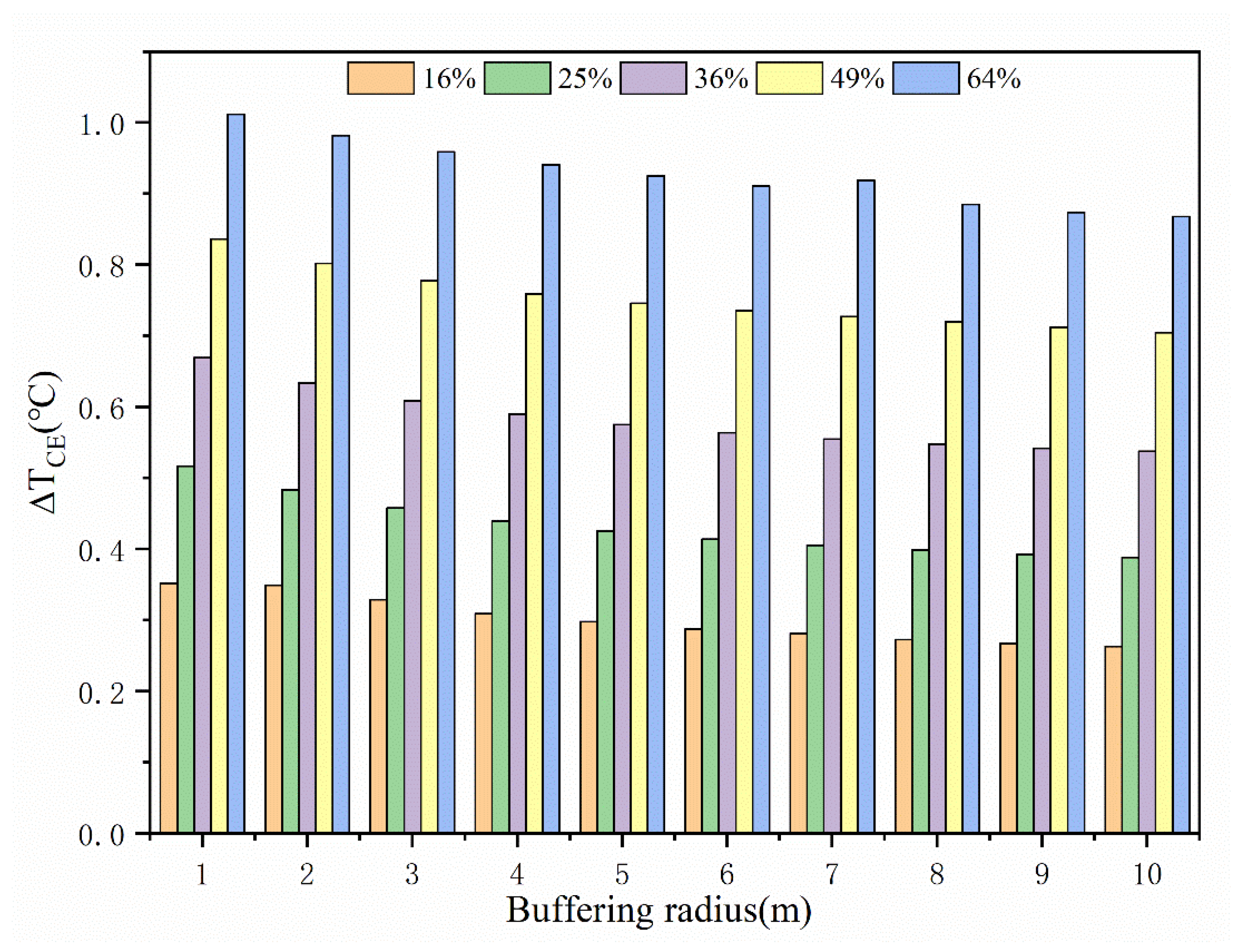
For a 1.4 m high horizontal surface, we set buffers at 1 m (model horizontal resolution) intervals to extract the average cooling effect of each buffer at 14:00. The cooling effect of different water body area proportions across a range of different buffers is shown in Figure 5. As the radius of the buffer increased, the cooling effect gradually decreased, and the cooling effect of the neighboring water body was the most obvious. Within the same buffer radius, the cooling effect of the water body continued to show increases with increasing water body area proportion.
3.2. The Effect of Layout on the Cooling Effect
3.2.1. Effect of the SI of Water Bodies on the Cooling Effect
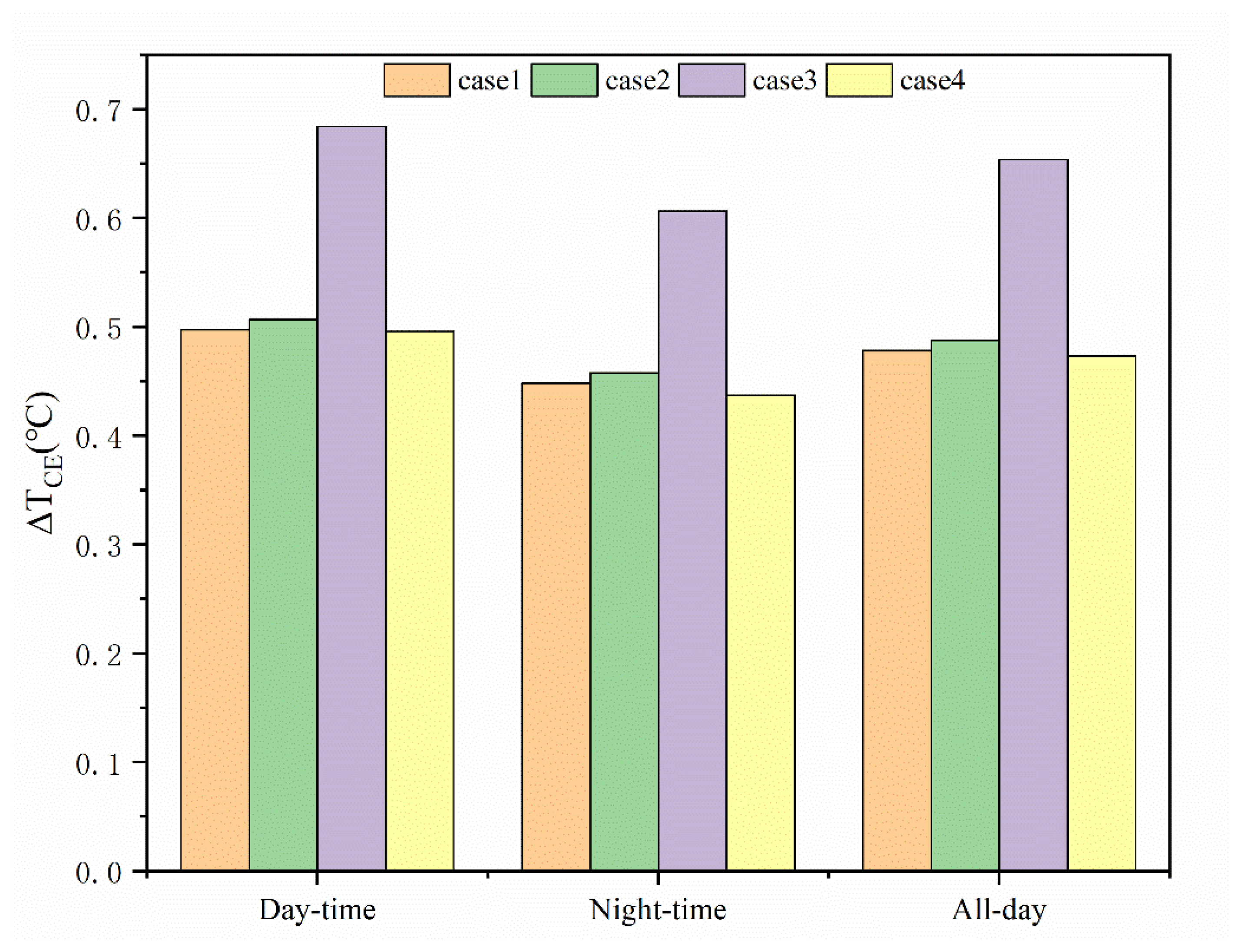
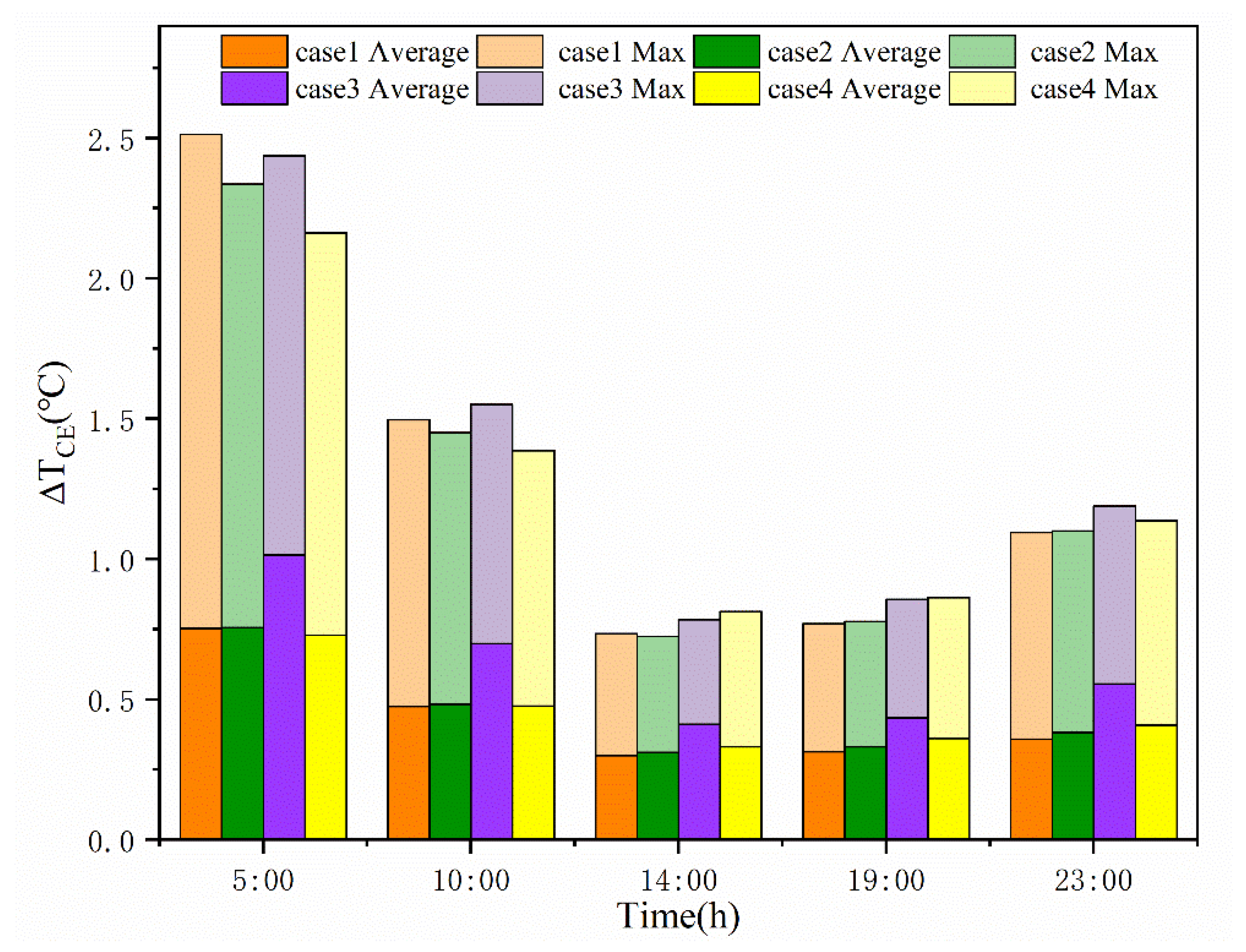
The distance between water patches affects the linkage of cooling effects between water patches. Thus, changing the distance between water patches can alter the cooling effect of water bodies. Cases 1, 2, 3, and 4 are shown in Figure 6 for daytime, nighttime, and all-day cooling effects. SI in case 3 was moderate and corresponded with a higher cooling effect during both day and night, making it the optimal layout among the four. Therefore, our analysis determined that the water body cooling effect would weaken if water body locations were too concentrated or too scattered. Additionally, moderate SI water bodies were more conducive to the linking of cooling effects between water patches. The average cooling effect and maximum cooling effect of water bodies with different SI values are shown in Figure 7. The dark color in Figure 7 represents the average value, and the light color represents the maximum value. There is no additive cooling effect presented in the figure, and the value provided as the maximum cooling effect is the value of the maximum cooling effect. The maximum cooling effect of case 1, the water body with the most concentrated layout, was 2.514 °C in the morning (5:00). The maximum cooling effect of case 3, with a moderate SI value, was better in the morning (10:00) and midnight (23:00), and the values of were 1.551 and 1.189 °C, respectively. In the afternoon (14:00) and evening (19:00), the cooling effect of case 4, with a higher SI value, was better, and the values of were 0.813 °C and 0.863, respectively. Regarding average cooling effect, case 3, with a moderate SI, had a higher cooling effect at all five typical time points. Therefore, we can infer that appropriately increasing the spacing of water patches aided in the reduction in temperature throughout the day within a locality.
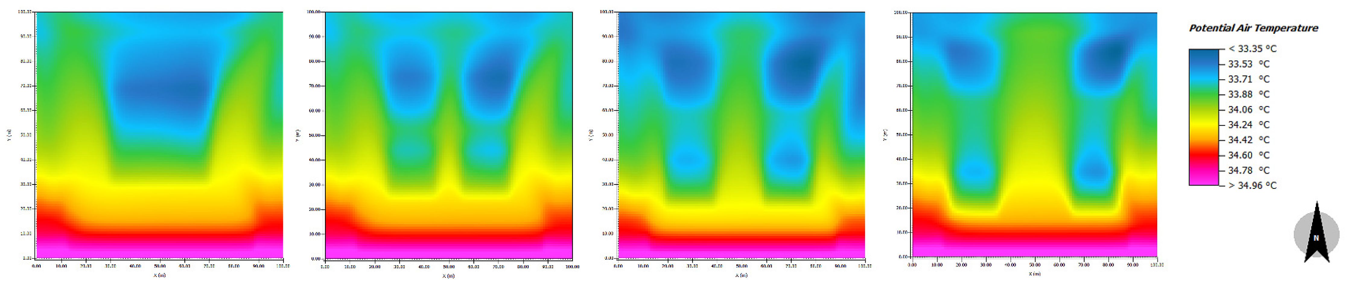
The temperature distribution of cases 1, 2, 3, and 4 at 14:00 is shown in Figure 8. We defined the blue area as the lowest-temperature area, the green and yellow areas as low-temperature areas, the orange and red areas as high-temperature areas, and the purple area as the highest-temperature area. From Figure 8, we can see that a moderate SI was more likely to reduce the temperature in the interstitial regions between water patches and had more cooling advantages for the whole location. As SI increased, the lowest-temperature region (blue) and the low-temperature region (green) gradually separated. However, the cooling effect linkage between the water patches caused the separated interstitial area to be filled by the next-lowest temperature region (yellow). When the SI was too high, the gap area between the patches was again gradually encroached upon by the high-temperature area (orange), and the distance between the oversized patches destroyed the linkage of cooling effects.
3.2.2. Effect of the LSI of Water Bodies on the Cooling Effect
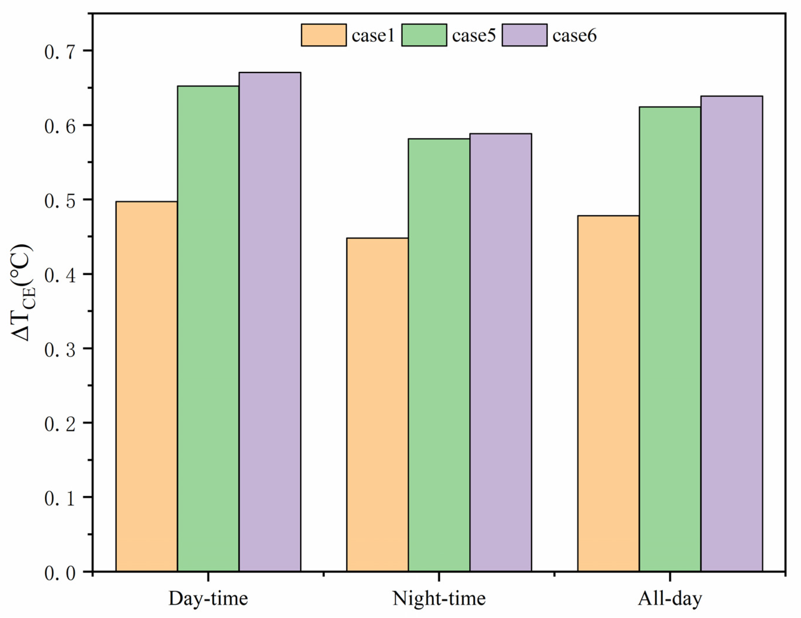
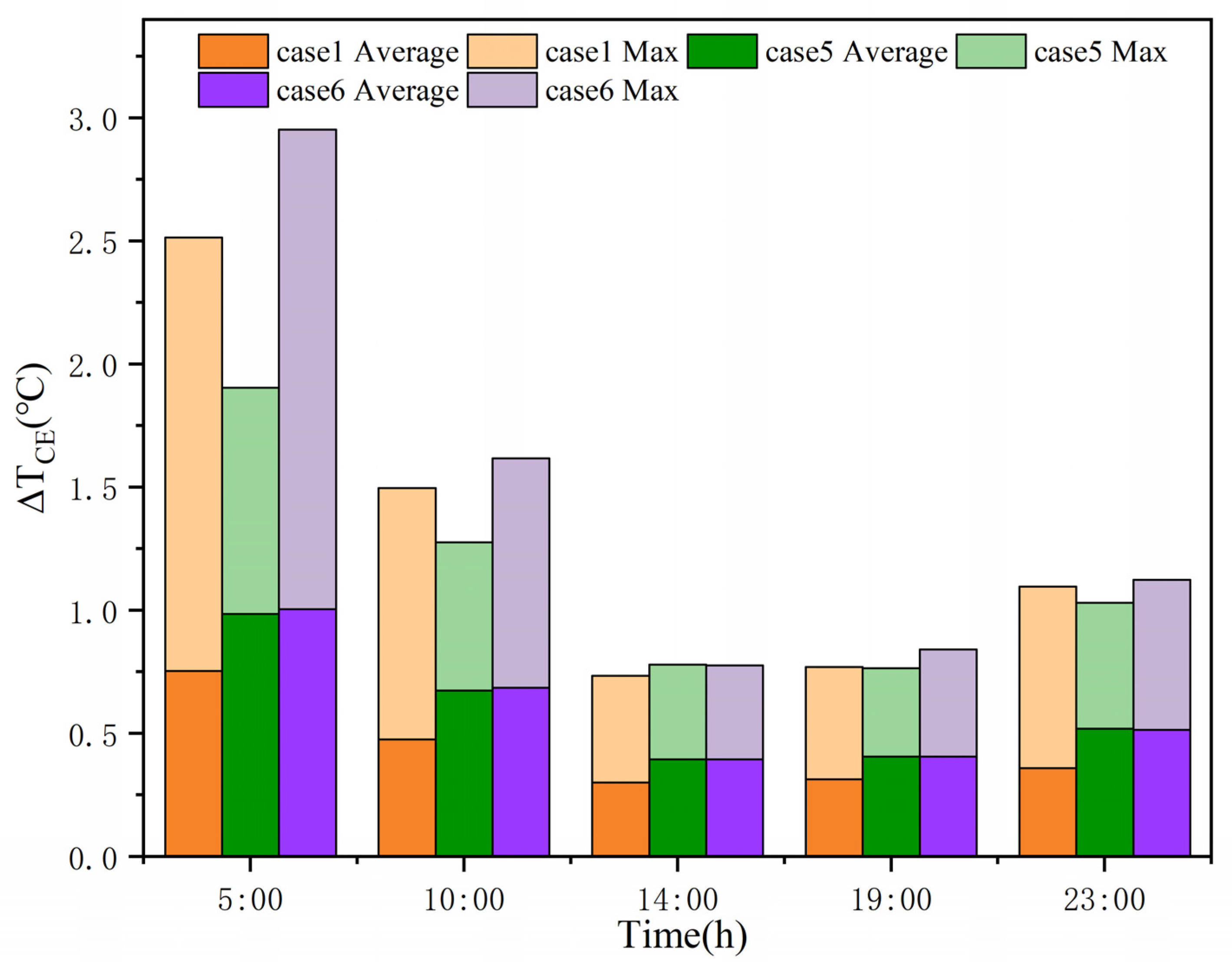
The cooling effect of water bodies is influenced not only by the cooling effect linkage between the patches but also by the characteristics of the water patches themselves, such as their shape. The daytime, nighttime, and all-day cooling effects for cases 1, 5, and 6 are shown in Figure 9. For water body layouts with the same LSI, the cooling effect of the water body at nighttime was more significant than that at daytime. Whether daytime or nighttime, the highest cooling effect was in case 6, and the lowest cooling effect was in case 1. We can see that the larger the LSI value for a water body, the higher the cooling effect. The average and maximum cooling effects of water bodies with different LSIs are shown in Figure 10. Case 6 had the highest maximum cooling effect. However, the maximum cooling effect of case 5 was smaller than that of case 1 at all time observations except 14:00, which indicates that a linear water body was the least favorable to a cumulative cooling effect. Regarding the average cooling effect, the cooling effect of the water body was more obvious as LSI increased, indicating that increased complexity of the water body shape was beneficial to the overall cooling effect of the water body on the surrounding environment.
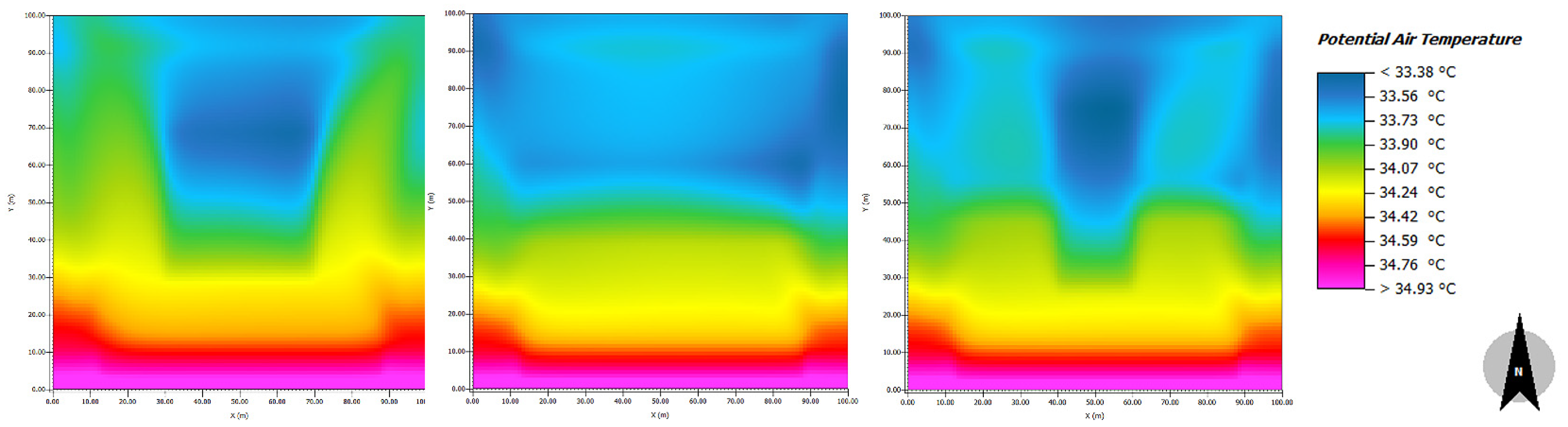
The temperature distribution for cases 1, 5, and 6 at 14:00 is shown in Figure 11. From Figure 11, we can see that as the shape index (LSI) increased, there was a clear tendency for the lowest-temperature area (blue) to deepen, with more areas within the locality displaying high cooling effect values. However, we simultaneously see that increases in the LSI weakened the uniformity of cooling within the locality, and the low-temperature area (green) was significantly reduced.
4. Discussion
4.1. The Effect of Wind Direction on the Cooling Effect
Just as water exerts a cooling effect on the air flowing over the water surface, the wind direction also influences the cooling effect of water bodies. From the temperature distribution experiment above, we can see that temperature was gradually reduced with changes in wind direction. When the water body was located in the windward area of the dominant wind direction in summer, the cooling effect of the water body could impact a larger area [22]. When the position of the water body is fixed, cold wind-driven air flowing over the water surface decreases the temperature in the downwind area significantly [35]. Therefore, we set points 1, 2, and 3 in cases where the area proportion of the water body was 16%, 25%, 26%, and 49% to study the cooling effect in the downwind area, center area, and upwind area of the water body. The location of each point is shown in Table 3.
The air temperatures and cooling effects for water bodies with different area proportions at 14:00 at the three points are shown in Table 4. We can see from Table 4 that the air temperature at the points in the downwind area was significantly lower than the air temperature at the points in the center and upwind areas of the water body when the area proportion of the water body was 16%, 25%, and 36%. The cooling effect in the downwind area was also significantly greater than that in the central and the upwind regions of the water body. However, the temperature and cooling effect in the central area of the water body was greater than that in the downwind and upwind areas when the area proportions of the water bodies were 49% and 64%. This indicates that the cooling effect on the surrounding environment gradually weakened when the area proportion of the water body was too large.
4.2. The Effect of Waterfront Green Space Type on the Cooling Effect
Waterfront green space acts as part of the water corridor and has a synergistic cooling effect with the water body. Waterfront green spaces can affect the radiation balance of water bodies by providing shade, lowering water temperature, and promoting air convection to reduce coastal temperature [36]. The spatial configuration and vegetation type of waterfront green spaces jointly affect the cooling effect. Vegetation configuration includes the variation among vegetation species and the selection and combination of tree, hedge, and grass types to form a multilevel vegetation structure [37]. To study the cooling effect of different vegetation types on the environment around water bodies, we constructed three ideal waterfront green space scenarios with three configured vegetation types: trees (height 15 m), hedges (height 2 m), and grasses (height 0.25 m). Apart from the water bodies, the underlying surface was set up as bare soil, and a no-green-space scenario was also considered, as shown in Table 5. The area proportion of the water body was 16%, and the coverage of the green areas was 33%.
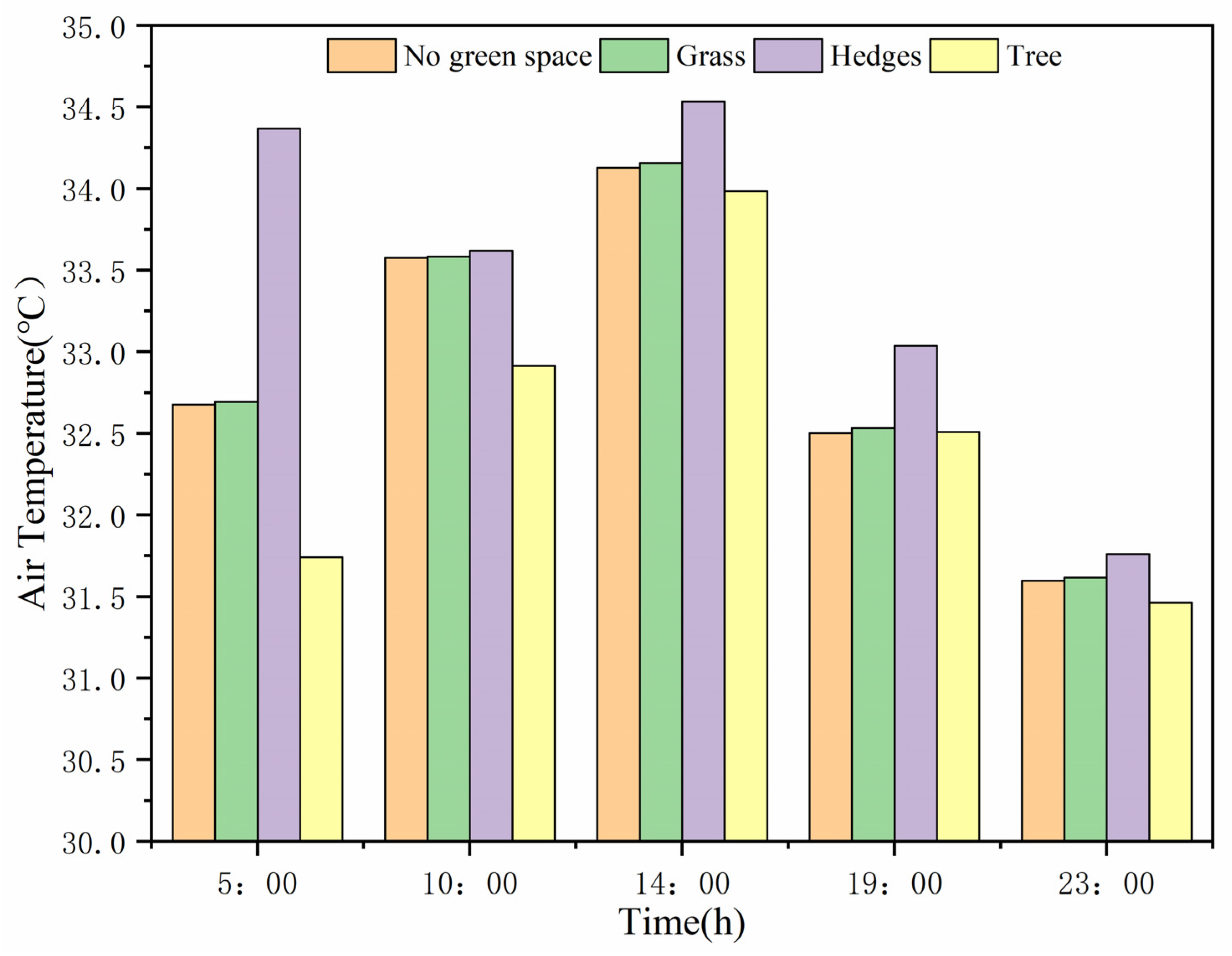
The air temperatures at five typical times for the four selected riparian vegetation type scenarios are shown in Figure 12. We can see from Figure 12 that the highest temperature at each observation was when hedges were the waterfront vegetation type, and the lowest temperature was when trees were the waterfront vegetation type. When grass and hedge were the vegetation type, the temperature was slightly higher than in the no-green-space scenario. Therefore, we can select trees as the optimum vegetation type for waterfront vegetation type selection.
The full-day cooling effect on localities with trees as the waterfront vegetation type relative to localities without greenery is shown in Figure 13. The cooling effect gradually increased before 8:00, and the strongest cooling effect was 1.457 °C at 8:00. The cooling effect gradually decreased after 8:00, and the weakest cooling effect was 0.011 °C at 17:00. The cooling effect of trees gradually disappeared after 17:00 because the shading and transpiration effect of the tree canopy gradually decreases following sunset, which weakens the cooling effect provided by trees.
5. Conclusions
The cooling effect of urban water bodies is influenced by several variables, including water body scale and layout pattern, which are important factors that cannot be ignored. We used the urban microclimate simulation software ENVI-met to construct models of different proportions and layouts of water bodies in order to analyze urban water bodies quantitatively. By analyzing the cooling effect of different water body proportions and layouts, we found that both elements significantly affect the cooling effect.
Our study verifies previous findings that the cooling effect of water bodies is correlated with scale, and larger water body proportions induce more pronounced cooling effects [21,35,38]. A large area of water usually has a high water convection heat dissipation capacity, which can significantly reduce the surrounding ambient temperature. When the water body area proportion was 16–64%, the all-day cooling effect was 0.48–1.57 °C. As the area proportion of a water body increases, its thermal storage capacity is enhanced, which further promotes heat transfer between the water body and the surrounding area, thus reducing the surrounding temperature. When the area of the water body was too small, it did not provide a cooling effect, which verifies the previous study results [39]. However, it is impossible to meet the demand for the urban cooling effect by increasing the area of water bodies. This is because as the area of the water body increases, the efficiency of the cooling effect of the water body decreases. When the area of the water body was too large, the cooling effect was most apparent in the center of the water body, and the cooling effect in the upwind and downwind directions was smaller than in the center of the water body.
Proper separation of water bodies can reduce the temperature of the areas between water bodies, and the linkage of cooling effects between water bodies can more evenly distribute the cooling effect across the locality. However, when the SI was high, the cooling effect linkages between the water patches disappeared. Therefore, the separation of water bodies in the same area should be appropriately increased to maximize the cooling benefit. Additionally, complex water body shapes had a more obvious cooling effect, and increasing the complexity of the shape increased the overall cooling effect of the water body on the surrounding environment [40,41].
In addition, wind direction and waterfront vegetation type also significantly affected water bodies’ cooling effects. When the water body area proportion was moderate, its cooling effect in the downwind area was higher than that in the center and the upwind areas. The cooling effect in the central area of the water body was higher than that in the upwind and downwind areas when the area proportion of the water body is larger. Regarding waterfront vegetation type, the cooling effect was most significant when the vegetation type was trees. The cooling effect of trees was most significant at 8:00 but disappeared after 18:00.
However, there are some limitations to this study. We only used a single form of numerical simulation data to analyze the cooling effects of different water bodies on the local thermal environment at the microscale. We did not use onsite measurements or remote sensing monitoring data to compare with numerical simulation data. Therefore, in subsequent research, we need to combine various methods to analyze the cooling effects of different water bodies from multiple proportions. Because the high summer temperature in Beijing includes high-frequency seasonal variability that affects the study of the cooling effect of water bodies, we used typical summer weather in Beijing as the meteorological conditions of the model. However, the water body cooling effect may vary in different regions with different summer meteorology. Thus, research on variation patterns in different regions should be continued. Not only would the factors of the water body itself affect the cooling effect, but also the type, material, and layout of the features around the water body, which would have a synergistic effect with the water’s cooling effect. However, we added only green areas and simple vegetation types with the same coverage around water bodies, and other factors were not considered. Therefore, the coupling effects of various factors should be studied in depth to analyze more complex cooling mechanisms.
Author Contributions
Conceptualization, B.C. and Q.C. (Qiang Chen); methodology, B.C.; software, B.C.; validation, B.C., Q.C. (Qianhao Cheng) and Y.L.; formal analysis, B.C.; investigation, B.C.; resources, Q.C. (Qiang Chen); data curation, R.L.; writing—original draft preparation, B.C.; writing—review and editing, Q.C. (Qiang Chen); visualization, B.C.; supervision, Q.C. (Qiang Chen); project administration, M.D.; funding acquisition, Q.C. (Qiang Chen). All authors have read and agreed to the published version of the manuscript.
Funding
This study is sponsored by the BUCEA Post Graduate Innovation Project, grant number PG2022107, the Pyramid Talent Training Project of Beijing University of Civil Engineering and Architecture, grant number JDYC20200321, and the General project of Beijing Municipal Science and Technology Commission, grant number KM201910016006.
Institutional Review Board Statement
Not applicable.
Informed Consent Statement
Not applicable.
Data Availability Statement
The data that support the findings of this study are available from the author upon reasonable request.
Acknowledgments
The authors would like to thank the editors and anonymous reviewers for their valuable time and efforts in reviewing this manuscript.
Conflicts of Interest
The authors declare no conflict of interest.
References
- Shi, D.; Song, J.; Huang, J.; Zhuang, C.; Guo, R.; Gao, Y. Synergistic cooling effects (SCEs) of urban green-blue spaces on local thermal environment: A case study in Chongqing, China. Sustain. Cities Soc. 2020, 55, 102065. [Google Scholar] [CrossRef]
- Gunawardena, K.R.; Wells, M.J.; Kershaw, T. Utilising green and bluespace to mitigate urban heat island intensity. Sci. Total Environ. 2017, 584, 1040–1055. [Google Scholar] [CrossRef] [PubMed]
- Tan, X.; Sun, X.; Huang, C.; Yuan, Y.; Hou, D. Comparison of cooling effect between green space and water body. Sustain. Cities Soc. 2021, 67, 102711. [Google Scholar] [CrossRef]
- Doick, K.J.; Peace, A.; Hutchings, T.R. The role of one large greenspace in mitigating London’s nocturnal urban heat island. Sci. Total Environ. 2014, 493, 662–671. [Google Scholar] [CrossRef]
- Jim, C.Y.; Chan, M.W.H. Urban greenspace delivery in Hong Kong: Spatial-institutional limitations and solutions. Urban For. Urban Green. 2016, 18, 65–85. [Google Scholar] [CrossRef]
- Wu, C.; Li, J.; Wang, C.; Song, C.; Chen, Y.; Finka, M.; La Rosa, D. Understanding the relationship between urban blue infrastructure and land surface temperature. Sci. Total Environ. 2019, 694, 133742. [Google Scholar] [CrossRef]
- Chang, C.R.; Li, M.H.; Chang, S.D. A preliminary study on the cool-island intensity of Taipei city parks. Landsc. Urban Plan. 2007, 80, 386–395. [Google Scholar] [CrossRef]
- Costanza, R.; d’Arge, R.; De Groot, R.; Farber, S.; Grasso, M.; Hannon, B.; Limburg, K.; Naeem, S.; O’neill, R.V.; Paruelo, J. The value of the world’s ecosystem services and natural capital. Nature 1997, 387, 253–260. [Google Scholar] [CrossRef]
- Cao, X.; Onishi, A.; Chen, J.; Imura, H. Quantifying the cool island intensity of urban parks using ASTER and IKONOS data. Landsc. Urban Plan. 2010, 96, 224–231. [Google Scholar] [CrossRef]
- Nicholson, S.E. Land surface atmosphere interaction: Physical processes and surface changes and their impact. Prog. Phys. Geogr. 1988, 12, 36–65. [Google Scholar] [CrossRef]
- Jia, H.; Ma, H.; Wei, M. Urban wetland planning: A case study in the Beijing central region. Ecol. Complex. 2011, 8, 213–221. [Google Scholar] [CrossRef]
- Karlessi, T.; Santamouris, M.; Synnefa, A.; Assimakopoulos, D.; Didaskalopoulos, P.; Apostolakis, K. Development and testing of PCM doped cool colored coatings to mitigate urban heat island and cool buildings. Build. Environ. 2011, 46, 570–576. [Google Scholar] [CrossRef]
- Syafii, N.I.; Ichinose, M.; Kumakura, E.; Chigusa, K.; Jusuf, S.K.; Wong, N.H. Enhancing the potential cooling benefits of urban water bodies. Nakhara J. Environ. Des. Plan. 2017, 13, 29–40. [Google Scholar]
- Peng, J.; Liu, Q.; Xu, Z.; Lyu, D.; Du, Y.; Qiao, R.; Wu, J. How to effectively mitigate urban heat island effect? A perspective of waterbody patch size threshold. Landsc. Urban Plan. 2020, 202, 103873. [Google Scholar] [CrossRef]
- Liu, Z.; Li, K.; Jia, H.; Wang, Z. Refining Assignment of Runoff Control Targets with a Landscape Statistical Model: A Case Study in the Beijing Urban Sub-Center, China. Water 2022, 14, 1466. [Google Scholar] [CrossRef]
- Qiu, W.; Xu, L. Thermal environment effect of urban water landscape. Acta Ecol. Sin. 2013, 33, 1852–1859. [Google Scholar]
- Li, C.; Yu, C.W. Mitigation of urban heat development by cool island effect of green space and water body. In Proceedings of the 8th International Symposium on Heating, Ventilation and Air Conditioning, Xi’an, China, 20–21 October 2013; pp. 551–561. [Google Scholar]
- Sun, R.; Chen, L. How can urban water bodies be designed for climate adaptation? Landsc. Urban Plan. 2012, 105, 27–33. [Google Scholar] [CrossRef]
- Cheng, L.; Guan, D.; Zhou, L.; Zhao, Z.; Zhou, J. Urban cooling island effect of main river on a landscape scale in Chongqing, China. Sustain. Cities Soc. 2019, 47, 101501. [Google Scholar] [CrossRef]
- Wang, Y.; Ouyang, W. Investigating the heterogeneity of water cooling effect for cooler cities. Sustain. Cities Soc. 2021, 75, 103281. [Google Scholar] [CrossRef]
- Sun, R.; Chen, A.; Chen, L.; Lue, Y. Cooling effects of wetlands in an urban region: The case of Beijing. Ecol. Indic. 2012, 20, 57–64. [Google Scholar] [CrossRef]
- Hong, J.; Teng, S.; Zhang, R. Effect of water body forms on microclimate of residential district. Energy Procedia 2017, 134, 256–265. [Google Scholar]
- Syafii, N.I.; Ichinose, M.; Kumakura, E.; Jusuf, S.K.; Hien, W.N.; Chigusa, K.; Ashie, Y. Assessment of the Water Pond Cooling Effect on Urban Microclimate: A Parametric Study with Numerical Modeling. Assessment 2021, 12, 461–471. [Google Scholar] [CrossRef]
- Amani-Beni, M.; Zhang, B.; Xu, J. Impact of urban park’s tree, grass and waterbody on microclimate in hot summer days: A case study of Olympic Park in Beijing, China. Urban For. Urban Green. 2018, 32, 1–6. [Google Scholar] [CrossRef]
- Li, S. Microclimate effects of different underlying surfaces in cities. In Proceedings of the 2006 Annual Meeting of China Meteorological Society, Chengdu, China, 25–27 October 2006; pp. 173–186. [Google Scholar]
- Anderson, W.P.; Anderson, J.L.; Thaxton, C.S.; Babyak, C.M. Changes in stream temperatures in response to restoration of groundwater discharge and solar heating in a culverted, urban stream. J. Hydrol. 2010, 393, 309–320. [Google Scholar] [CrossRef] [Green Version]
- Yu, K.; Chen, Y.; Liang, L.; Gong, A.; Li, J. Quantitative analysis of the interannual variation in the seasonal water cooling island (WCI) effect for urban areas. Sci. Total Environ. 2020, 727, 138750. [Google Scholar] [CrossRef]
- Sun, X.; Tan, X.; Chen, K.; Song, S.; Zhu, X.; Hou, D. Quantifying landscape-metrics impacts on urban green-spaces and water-bodies cooling effect: The study of Nanjing, China. Urban For. Urban Green. 2020, 55, 126838. [Google Scholar] [CrossRef]
- Manteghi, G.; Lamit, H.; Remaz, D.; Aflaki, A. ENVI-Met simulation on cooling effect of Melaka River. Int. J. Energy Environ. Res. 2016, 4, 7–15. [Google Scholar]
- Yang, J.; Hu, X.; Feng, H.; Marvin, S. Verifying an ENVI-met simulation of the thermal environment of Yanzhong Square Park in Shanghai. Urban For. Urban Green. 2021, 66, 127384. [Google Scholar] [CrossRef]
- Han, D.; Yang, X.; Cai, H.; Xu, X. Impacts of neighboring buildings on the cold island effect of central parks: A case study of Beijing, China. Sustainability 2020, 12, 9499. [Google Scholar] [CrossRef]
- Liu, Z.; Cheng, W.; Jim, C.Y.; Morakinyo, T.E.; Ng, E. Heat mitigation benefits of urban green and blue infrastructures: A systematic review of modeling techniques, validation and scenario simulation in ENVI-met V4. Build. Environ. 2021, 200, 107939. [Google Scholar] [CrossRef]
- Chen, Z. Simulation and optimization of the impact of green space on urban local thermal environment. Master’s Thesis, Beijing Normal University, Beijing, China, 2018. [Google Scholar]
- McGarigal, K. FRAGSTATS: Spatial Pattern Analysis Program for Quantifying Landscape Structure; U.S. Department of Agriculture, Forest Service, Pacific Northwest Research Station: St. Paul, MN, USA, 1995; Volume 351.
- Zeng, Z.; Zhou, X.; Li, L. The Impact of Water on Microclimate in Lingnan Area. Procedia Eng. 2017, 205, 2034–2040. [Google Scholar] [CrossRef]
- Herb, W.R.; Stefan, H.G. Dynamics of vertical mixing in a shallow lake with submersed macrophytes. Water Resour. Res. 2005, 41, 293–307. [Google Scholar] [CrossRef]
- Sodoudi, S.; Zhang, H.; Chi, X.; Müller, F.; Li, H. The influence of spatial configuration of green areas on microclimate and thermal comfort. Urban For. Urban Green. 2018, 34, 85–96. [Google Scholar] [CrossRef]
- Syafii, N.I.; Ichinose, M.; Kumakura, E.; Jusuf, S.K.; Chigusa, K.; Wong, N.H. Thermal environment assessment around bodies of water in urban canyons: A scale model study. Sustain. Cities Soc. 2017, 34, 79–89. [Google Scholar] [CrossRef]
- Jacobs, C.; Klok, L.; Bruse, M.; Cortesão, J.; Lenzholzer, S.; Kluck, J. Are urban water bodies really cooling? Urban Clim. 2020, 32, 100607. [Google Scholar] [CrossRef]
- Zhang, Q.; Wu, Z.; Chen, Y. Seasonal Variations of the Cooling Effect of Water Landscape in High-density Urban Built-up Area: A Case Study of the Center Urban District of Guangzhou. In Proceedings of the 2017 2nd International Conference on Frontiers of Sensors Technologies (ICFST), Shenzhen, China, 14–16 April 2017; pp. 394–400. [Google Scholar]
- Xue, Z.; Hou, G.; Zhang, Z.; Lyu, X.; Jiang, M.; Zou, Y.; Shen, X.; Wang, J.; Liu, X. Quantifying the cooling-effects of urban and peri-urban wetlands using remote sensing data: Case study of cities of Northeast China. Landsc. Urban Plan. 2019, 182, 92–100. [Google Scholar] [CrossRef]
Figure 1.
Maximum, minimum, and average temperatures at 14:00.

Figure 2.
Hourly temperature of water bodies with different area proportions throughout the day.

Figure 3.
Cooling effect and efficiency of the cooling effect for different water body area proportions.
Figure 3.
Cooling effect and efficiency of the cooling effect for different water body area proportions.

Figure 4.
The cooling effect of water bodies with different area proportions at different time points.
Figure 4.
The cooling effect of water bodies with different area proportions at different time points.

Figure 5.
Cooling effect of different water body area proportions in different buffer radii.

Figure 6.
Day-time, night-time, and all-day cooling effects in cases 1, 2, 3 and 4.

Figure 7.
Average cooling effect and maximum cooling effect of cases 1, 2, 3 and 4.

Figure 8.
Distribution of temperature in cases 1, 2, 3, and 4 at 14:00.

Figure 9.
Daytime, nighttime, and all-day cooling effects in cases 1, 5 and 6.

Figure 10.
Average cooling effect and maximum cooling effect in cases 1, 5 and 6.

Figure 11.
Distribution of temperature in cases 1, 5, and 6 at 14:00.

Figure 12.
The air temperature of different waterfront vegetation types at different time points.

Figure 13.
The hourly cooling effect of trees.


Table 1.
Different water body area proportions model settings.
| Water Body Area Proportion | Area (m²) | Model |
|---|---|---|
| 0% | 0 |  |
| 1% | 100 |  |
| 4% | 400 |  |
| 9% | 900 |  |
| 16% | 1600 |  |
| 25% | 2500 |  |
| 36% | 3600 |  |
| 49% | 4900 |  |
| 64% | 6400 |  |
Table 2.
Different water body layout model settings.
| Case | Perimeter of a Single Water Patch (m) | Area of a Single Water Patch (m²) | SI | LSI | Model |
|---|---|---|---|---|---|
| case 1 | 160 | 1600 | 0 | 1.13 |  |
| case 2 | 40 | 400 | 0.06 | 1.13 |  |
| case 3 | 40 | 400 | 0.25 | 1.13 |  |
| case 4 | 40 | 400 | 0.56 | 1.13 |  |
| case 5 | 200 | 1600 | 0 | 1.41 |  |
| case 6 | 260 | 1600 | 0 | 1.69 |  |
Table 3.
Distribution of points in each area.
| Water Body Area Proportion | 16% | 25% | 36% | 49% | 64% |
|---|---|---|---|---|---|
| Points |  |  |  |  |  |
Table 4.
Air temperature and cooling effect for each point.
| Water Body Area Proportion | Point | Air Temperature (°C) | Cooling Effect (°C) |
|---|---|---|---|
| 16% | 1 | 33.506 | 0.672 |
| 2 | 33.734 | 0.560 | |
| 3 | 34.245 | 0.199 | |
| 25% | 1 | 33.343 | 0.812 |
| 2 | 33.576 | 0.718 | |
| 3 | 34.197 | 0.298 | |
| 36% | 1 | 33.182 | 0.956 |
| 2 | 33.390 | 0.905 | |
| 3 | 34.139 | 0.416 | |
| 49% | 1 | 33.037 | 1.093 |
| 2 | 33.183 | 1.112 | |
| 3 | 34.094 | 0.555 | |
| 64% | 1 | 32.938 | 1.203 |
| 2 | 33.019 | 1.275 | |
| 3 | 34.146 | 0.686 |
Table 5.
Model settings for different waterfront vegetation types.
| Waterfront Green Space Type | No Green Space | Grass (0.25 m) | Hedges (2 m) | Tree (15 m) |
|---|---|---|---|---|
| Model |  |  |  |  |
Publisher’s Note: MDPI stays neutral with regard to jurisdictional claims in published maps and institutional affiliations. |
© 2022 by the authors. Licensee MDPI, Basel, Switzerland. This article is an open access article distributed under the terms and conditions of the Creative Commons Attribution (CC BY) license (https://creativecommons.org/licenses/by/4.0/).
Share and Cite
MDPI and ACS Style
Cao, B.; Chen, Q.; Du, M.; Cheng, Q.; Li, Y.; Liu, R. Simulation Analysis of the Cooling Effect of Urban Water Bodies on the Local Thermal Environment. Water 2022, 14, 3091. https://doi.org/10.3390/w14193091
AMA Style
Cao B, Chen Q, Du M, Cheng Q, Li Y, Liu R. Simulation Analysis of the Cooling Effect of Urban Water Bodies on the Local Thermal Environment. Water. 2022; 14(19):3091. https://doi.org/10.3390/w14193091
Chicago/Turabian StyleCao, Beilei, Qiang Chen, Mingyi Du, Qianhao Cheng, Yuanyuan Li, and Rui Liu. 2022. "Simulation Analysis of the Cooling Effect of Urban Water Bodies on the Local Thermal Environment" Water 14, no. 19: 3091. https://doi.org/10.3390/w14193091
Note that from the first issue of 2016, this journal uses article numbers instead of page numbers. See further details here.