Article

Theoretical Model and Experimental Research on Determining Aquifer Permeability Coefficients by Slug Test under the Influence of Positive Well-Skin Effect

1
School of Earth Sciences and Engineering, Hohai University, Nanjing 210098, China
2
China Water Resources Beifang Investigation, Design and Research Co., Ltd., Tianjin 300222, China
*
Author to whom correspondence should be addressed.
Water 2022, 14(19), 3089; https://doi.org/10.3390/w14193089
Submission received: 20 August 2022 / Revised: 23 September 2022 / Accepted: 25 September 2022 / Published: 1 October 2022

Abstract

:
In the process of slug test in the field, mud and debris may infiltrate into the aquifer during the formation of the test well, and a poorly permeable annulus area appears around the test well wall. This is called the positive well-skin effect, which can have a significant impact on the results of slug tests due to the characteristics of a slug test. Therefore, to carry out the research on the determination of aquifer permeability coefficients by slug test under the influence of positive well-skin effect, a mathematical model of a slug test considering the positive well-skin effect was constructed. The Laplace transform method and the AWG algorithm were used to solve for a series of standard curves, and specific steps were given for calculating aquifer permeability coefficients by slug test under the influence of positive well-skin effect. Meanwhile, an indoor test model with positive well-skin effect was constructed, then several sets of slug tests and pumping tests with different excitation strengths were carried out. Based on this study, the presence of positive well-skin layer had a great impact on the aquifer permeability coefficient determined from both the pumping test and Kipp model of slug test, resulting in smaller results. The HWS model overcomes the influence of positive well-skin effect. This will further improve the theory of slug test, increase the accuracy of slug test in determining the permeability coefficient, and promote the application scope of slug test. It is therefore possible to discern the well-skin factor and determine the aquifer permeability coefficient by fitting the slug test data to a standard curve.

1. Introduction

As an efficient technique for testing the permeability coefficients of aquifers, the slug test is characterized by short test cycle, simple equipment, and high accuracy [1]. Hvorslev [2], Cooper [3], Bouwer and Rice [4], Kipp [5], McElwee [6], Huang [7], Zhou [8], Zhao [9,10,11], and Liang [12] all proposed theoretical models and engineering applications for the slug test in determining hydrogeological parameters of aquifers, none of which have considered the well-skin effect.
However, in the actual application of the slug test, it is likely that a positive well-skin effect appears due to the inevitable influence of factors such as mud wall protection during the drilling. Based on the mechanism characteristics of slug test, this positive well-skin effect greatly affects the accuracy of the slug test and thus has become a technical bottleneck limiting the application of slug test to a large extent. Meanwhile, current methods to reduce the influence of well-skin effect on permeability still focus on how to eliminate the presence of well-skin effect, and while the test results are slightly more accurate, they are costly and inefficient. As a result, various research on the influences of well-skin effect on the slug test have been carried out at home and abroad. Back in 1972, Ramey et al. [13] were the first to propose a theoretical model for slug test that took into account the well-skin effect. They assumed that the well-skin layer was extremely thin, with boundaries extending to infinity, and that the water storage effect of the well was taken into consideration. A series of standard curves were obtained to determine the permeability coefficient of the aquifer and well-skin effect based on the relationship between the dimensionless water storage coefficient and factors related to the well-skin effect. The model considers a more comprehensive situation, but the similarity of the standard curve shapes leads to a high degree of uncertainty in determining the relevant parameters. As a result, this fitting method may lead to inaccurate estimates of aquifer permeability coefficients. Faust [14] investigated the effect of well-skin of finite thickness on the results of the slug test using a numerical model and a simple analytical solution. The results show that the data obtained from the slug test are more representative of the permeability coefficient of the well-skin layer rather than that of the aquifer. The reason is that when well-skin of finite thickness is existent, the curve of the slug test results is shifted along the horizontal axis, making the estimation of the permeability coefficient unreliable. Moench [15] summarized the existing theoretical models of the slug test and pointed out the relationship between the two assumptions of infinitely thin and finitely thick well-skins; the solution for a finite-thickness well-skin is equal to the solution for an infinitely thin well-skin with the storage effect of the well-skin neglected. Sageev [16] assumed well-skin layer existed with extremely thin thickness. Considering the storage effect of the well bore, it was found that when solving for aquifer permeability coefficients with the matching line method, the measured curves should be analysed in three periods: early, middle, and late. The early period mainly reflects the permeability coefficient of well-skin layer, the middle period curve is suitable to the case where there is no well-skin, and the late period curve can be used when well-skins are positive or when the well-skin effect is not considered. Song [17] and Zeng [18] analysed the slug test results under the influence of well-skin effect, divided the slug test process into initial and intermediate stages, and developed a two-stage analysis method to estimate the well-skin factor S w and aquifer permeability coefficient K a . In a slug test conducted by Rovey II [19] and others on 31 test wells of varying development strength in porous alluvium, a link was found between the well-skin effect and the development strength of the test wells, with the test results being small due to the presence of a positive well-skin effect rather than wellbore damage. The results were also analysed with the means of conventional Bouwer–Rice method and the deconvolution method, which quantifies and removes some degree of well-skin effect. Barrash et al. [20] founded the cause of positive well-skin effect and the evidence of head loss through observation and analysis results of a large number of tests in the BHRS research base: compaction, residue invasion, and blockage of screen. Yeh et al. [21] proposed a simulation method to estimate the thickness of well-skin layer and other hydraulic parameters at the same time and used the annealing (SA) algorithm to estimate five parameters: hydraulic conductivity, specific storage and thickness of the well-skin layer, hydraulic conductivity, and specific storage of the aquifer. Chen [22] first compared the slug test with the conventional pumping test and found that the slug test has very obvious advantages and that it causes less groundwater disturbance, but the radius of influence of slug test is basically within 10 m and only represents a small area of stratigraphic properties near the test well, and the slug test has high requirements on the quality of test well structure and is susceptible to the well-skin effect. To address this drawback, he concluded that the test well structure needs to be pre-designed and adequately washed before the test. Ju [23] carried out pumping test and slug test in the field, and the test results showed that the pumping test involved a large area, while the slug test involved a small area, and the K value of the pumping test was 1.5 times higher than that of the slug test. The well-skin effect was the main reason that leads to the difference between the two test results. Cardiff et al. [24] considered that due to slug tests’ high sensitivity to low-conductivity skins, it was possible that aquifer K estimates obtained may simply represent depth-variability in a low-conductivity skin. By comparing K profiles obtained at closely-spaced wells, the volume being interrogated by the slug test response extended beyond the wellbore skin and represented true aquifer K variability. Sahin [25] proposed that the influence of the well-skin effect must be considered when calculating aquifer permeability parameters in slug tests and that slug test results that took into account the influence of the well-skin effect were more reliable and accurate. Weeks [26] proposed that the well-skin effect had a significant impact on the test results of the slug test, affecting parameters related to the permeability parameters and the water storage coefficient. Liu [27] used numerical approaches to propose a new three-dimensional slug test model for inhomogeneous aquifers in which inertia effects associated with linear friction and well-skin effect are considered. Morozov [28] evaluated aquifer anisotropic permeability and well-skin effect based on slug test data in incomplete wells.
In previous studies, most of the studies on slug test under positive well-skin effect used numerical simulation or parameter inversion of a large number of test data to estimate the aquifer permeability coefficient. There was no good method to accurately calculate the permeability coefficient of well-skin layer, nor was there a special large-scale physical test model to carry out the research of slug test under the positive well-skin effect to determine the aquifer permeability coefficient, so the mechanism research of the well-skin effect on the slug test is lacking. Therefore, it is necessary to study the hydraulic conductivity between the aquifer and the well-skin from the perspective of the mechanism of the well-skin effect. In this study, the mathematical model of the slug test under the positive well-skin effect is firstly proposed; the standard curve of the model was obtained by solving with Laplace transform and AWG (Azari–Wooden–Gaver) algorithm, and the corresponding specific calculation steps of the model based on the solution process are given. Meanwhile, the physical test model was constructed indoors, based on data from multiple sets of slug tests and pumping tests with different excitation strengths, the reliability and accuracy of the proposed theory and method for determining aquifer permeability coefficients by slug test under positive well-skin effects (HHU-Well-Skin model, whose abbreviation is HWS model) was verified by comparing the calculation results with those of the pumping tests and Kipp model method. This will further improve the theory of the slug test, increase the accuracy of the slug test in determining the permeability coefficient, and promote the scope of application of the slug test.

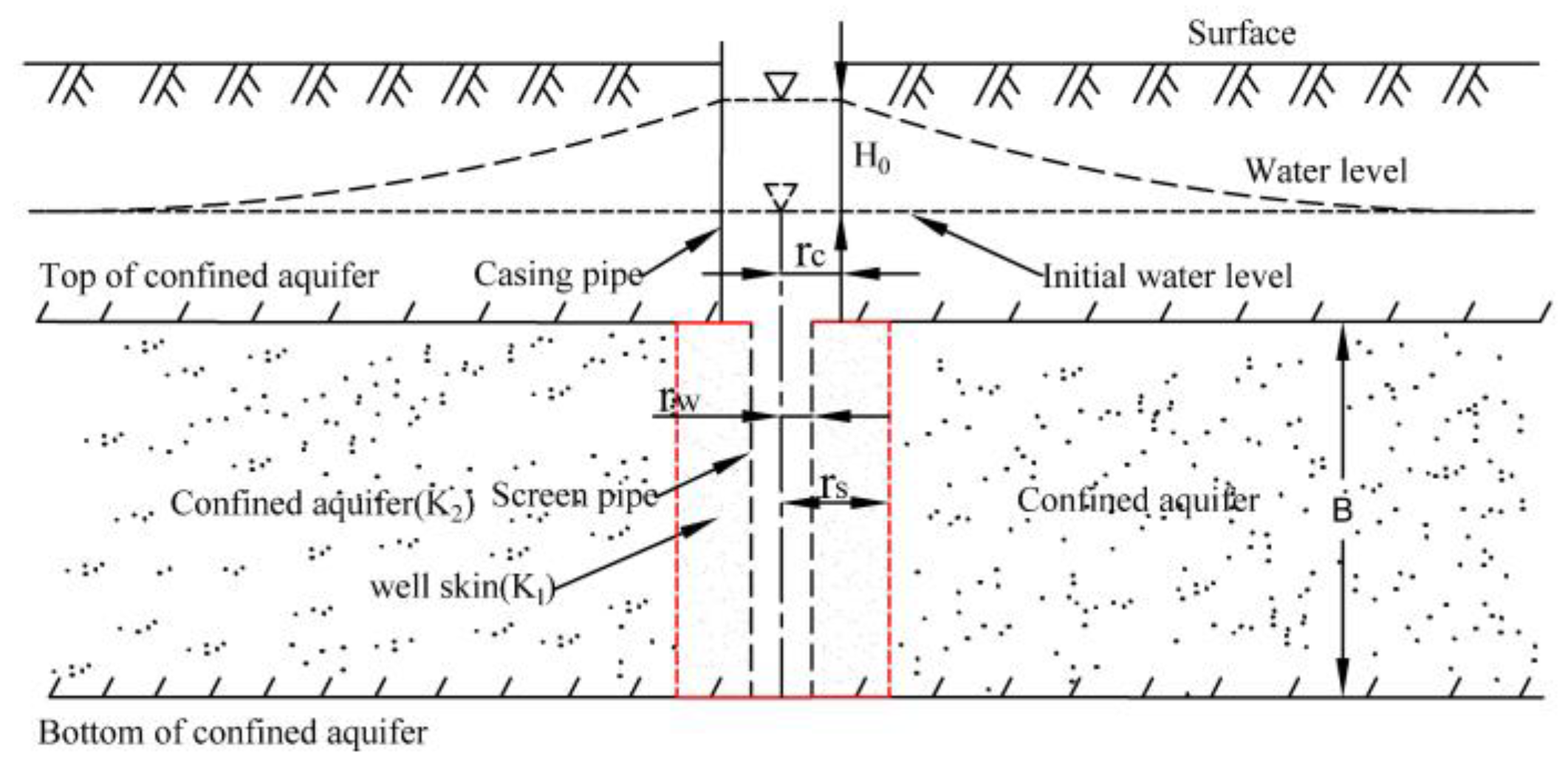
2. Theoretical Model Construction for Slug Test under Positive Well-Skin Effect (HSW Model)

2.1. Basic Condition Assumptions

(1) The aquifer is a confined aquifer of constant thickness and horizontal occurrence, with a homogeneous and isotropic medium; (2) groundwater flowing in the aquifer is radial; (3) there is a well-skin layer of finite thickness, and the distance from the centre of the well to the outer boundary of the well-skin layer is r s ; (4) head friction losses are negligible; and (5) the test well is a complete well.

2.2. Establishment and Solution of Model

The continuity equation was established in the confined aquifer and finite thickness well-skin layer; the water balance equation was established in the contact surface between the confined aquifer and the finite thickness well-skin layer and between the finite thickness well-skin layer and the well. The theoretical model of the slug test under the positive well-skin effect was thus constructed, and the aquifer structural model of the slug test under the positive well-skin effect is shown in Figure 1.
(1) Establishment of the theoretical model
In the confined complete well system, the governing equation of groundwater radial flow in a well-skin layer and a confined aquifer is:
2 h 1 r 2 + 1 r h 1 r = S 1 K 1 h 1 t ,     r w r r s
2 h 2 r 2 + 1 r h 2 r = S 2 K 2 h 2 t , r s r
A water balance equation is established in the contact surface between the confined aquifer and the well-skin layer of finite thickness:
K 1 h 1 ( r s , t ) r = K 2 h 2 ( r s , t ) r , t > 0
A water balance equation is established in the contact surface between the well-skin layer of finite thickness and the well:
π r c 2 d H ( t ) d t = 2 π r w K 1 B h 1 ( r w , t ) r , t > 0
Initial conditions:
h 1 ( r , 0 ) = h 2 ( r , 0 ) = 0 , r > r w
H ( 0 ) = H 0
Boundary conditions:
h 2 ( , t ) = 0
h 1 ( r s , t ) = h 2 ( r s , t ) , t > 0
H ( t ) = h 1 ( r w , t )
Among them, subscripts 1 and 2 represent well-skin layer and confined aquifer parameters, respectively; h is the value of head change ( m ) ;   r is the distance from a point within the well-skin layer or aquifer to the centre of the well ( m ) ; t is time ( s ) ; K is the permeability coefficient ( m · d 1 ) ; S is the water storage coefficient; r w is the radius of the screen pipe ( m ) ; r c is the radius of the well casing ( m ); r s is the distance from the centre of the well to the outer boundary of the well-skin layer ( m ) ; B is the thickness of the confined aquifer ( m ) ; and H ( t ) is the change of well water level at time t relative to the initial water level ( m ) .
(2) Solution of the theoretical model
First, the equations and the definite solution conditions were transformed into dimensionless models by dimensionless factors and parametric variables, and then, in turn, the Laplace transform was performed. The dimensionless transformation equation is:
h 1 D = h 1 H 0 , h 2 D = h 2 H 0 , ρ = r r w , ρ s = r s r w , ρ w = 1 , τ = K 2 t S 2 r w 2 , α = K 2 K 1 , β = S 1 K 2 S 2 K 1 , γ = r c 2 2 S 2 B r w 2
The results are as follows after Laplace transformations of time in Equations (1) and (2):
2 h 1 D ¯ ρ 2 + 1 ρ h 1 D ¯ ρ β 2 p h 1 D ¯ = 0 ,   1 ρ ρ s
2 h 2 D ¯ ρ 2 + 1 ρ h 2 D ¯ ρ p h 2 D ¯ = 0 ,   ρ s ρ
Then, Equations (3) and (4) are, respectively, converted to:
h 1 D ¯ ρ ( ρ s , p ) = α h 2 D ¯ ρ ( ρ s , p ) ,   p > 0
α γ ( p H D ¯ 1 ) = h 1 D ¯ ( 1 , p ) ρ
The conditional Equations of definite solution (7)–(9) are, respectively, converted to:
h 2 D ¯ ( , p ) = 0 , p > 0
h 1 D ¯ ( ρ s , p ) = h 2 D ¯ ( ρ s , p ) ,   p > 0
According to the modified Bessel equation of order 0,
d 2 y d x 2 + 1 x d y d x β 2 y = 0
The general solution of Equation (17) is:
y = C 1 K 0 ( β x ) + C 2 I 0 ( β x )
Among them, I 0 ( x ) and K 0 ( x )   are the first and second type of modified Basel functions, respectively; C 1   and   C 2   are two constants determined by the boundary conditions. Therefore, according to the general solution of Equation (17), the solutions of Equations (11) and (12) can be obtained as:
h 1 D ¯ ( ρ , p ) = C 1 K 0 ( β ρ p ) + C 2 I 0 ( β ρ p )
h 2 D ¯ ( ρ , p ) = C 3 K 0 ( ρ p ) + C 4 I 0 ( ρ p )
Among them, C 1   and C 2   as well as C 3   and C 4   are constants determined by boundary conditions in well-skin layers and aquifer, respectively.
According to Equation (15),
lim ρ h 2 D ¯ ( ρ , p ) = 0
The first type of modified Bessel function I 0 ( x ) is an exponentially growing function with the property that when x , I 0 ( x ) , so C 4 = 0 in Equation (21).
h 2 D ¯ ( ρ , p ) = C 3 K 0 ( ρ p )
According to Equation (13),
C 1 K 0 ( β ρ s p ) + C 2 I 0   ( β ρ s p ) = C 3 K 0 ( ρ s p )
For
h 1 D ¯ ρ ( ρ s , p ) = h 1 D ¯ ρ ( ρ , p ) | ρ = ρ s = C 1 β p K 0 ( β ρ s p ) ( β ρ s p ) + C 2 β p I 0 ( β ρ s p ) ( β ρ s p )
α h 2 D ¯ ρ ( ρ s , p ) = α h 2 D ¯ ρ ( ρ , p ) | ρ = ρ s = α C 3 p K 0 ( ρ s p ) ( ρ s p )
By the properties of the modified Bessel equation of order 0,
d d x K 0 ( x ) = K 1 ( x )
d d x I 0 ( x ) = I 1 ( x )
Therefore, Equations (25) and (26) are:
C 1 β p K 0 ( β ρ s p ) ( β ρ s p ) + C 2 β p I 0 ( β ρ s p ) ( β ρ s p )   = C 1 β p K 1 ( β ρ s p ) + C 2 β p   I 1 ( β ρ s p )
α C 3 p K 0 ( ρ s p ) ( ρ s p ) = α C 3 p K 1 ( ρ s p )
Therefore, according to the Equations (16), (25), (26), (28), and (29), the following conclusions can be obtained:
C 1 β p K 1 ( β ρ s p ) + C 2 β p I 1 ( β ρ s p ) = α p C 3 K 1 ( ρ s p )
Simplification of Equation (30):
C 1 β K 1 ( β ρ s p ) C 2 β I 1 ( β ρ s p ) = α C 3 K 1 ( ρ s p )
For
p H D ¯ ( ρ ) 1 = p h 1 D ¯ ( 1 , p ) 1 = p [ C 1 K 0 ( β p ) + C 2 I 0 ( β p ) ] 1
According to Equations (25) and (29),
h 1 D ¯ ρ ( 1 , p ) = h 1 D ¯ ρ ( ρ , p ) | ρ = 1 = C 1 β p K 1 ( β p ) + C 2 β p I 1 ( β p )
Associating Equations (32) and (33) according to Equation (14),
α γ [ p ( C 1 K 0 ( β p ) + C 2 I 0 ( β p ) ) 1 ] = C 1 β p K 1 ( β p ) + C 2 β p I 1 ( β p )
According to Equation (34),
C 1 = α γ + C 2 [ β I 1 p ( β p ) α γ p I 0 ( β p ) ] α γ p K 0 ( β p ) + β p K 1 ( β p )
Equation (24) × α K 1 ( ρ s p )   and Equation (31) × K 0 ( ρ s p ) , respectively:
C 1 α K 0 ( β ρ s p ) K 1 ( ρ s p ) + C 2 α I 0 ( β ρ s p ) K 1 ( ρ s p ) = C 3 α K 0 ( ρ s p ) K 1 ( ρ s p )
C 1 β K 1 ( β ρ s p ) K 0 ( ρ s p ) C 2 β I 1 ( β ρ s p ) K 0 ( ρ s p ) = C 3 α K 1 ( ρ s p ) K 0 ( ρ s p )
The solution of combining Equations (36) and (37) is:
C 1 = C 2 [ α I 0 ( β ρ s p ) K 1 ( ρ s p ) β I 1 ( β ρ s p ) K 0 ( ρ s p ) ] α K 0 ( β ρ s p ) K 1 ( ρ s p ) β K 1 ( β ρ s p ) K 0 ( ρ s p )
From Equations (35) and (38),
[ α I 0 ( β ρ s p ) K 1 ( ρ s p ) + β I 1 ( β ρ s p ) K 0 ( ρ s p ) ] × [ α γ p K 0 ( β p ) + β p K 1 ( β p ) ] C 2 [ β p I 1 ( β p ) α γ p I 0 ( β p ) ] × [ β K 1 ( β ρ s p ) K 0 ( ρ s p ) α K 0 ( β ρ s p ) K 1 ( ρ s p ) ] C 2 = [ β K 1 ( β ρ s p ) K 0 ( ρ s p ) α K 0 ( β ρ s p ) K 1 ( ρ s p ) ] × α γ
Set:
a 1 = α γ p I 0 ( β p ) β p I 1 ( β p )
a 2 = α γ p K 0 ( β p ) + β p K 1 ( β p )
c 1 = α I 0 ( β ρ s p ) K 1 ( ρ s p ) + β I 1 ( β ρ s p ) K 0 ( ρ s p )
c 2 = β K 1 ( β ρ s p ) K 0 ( ρ s p ) α K 0 ( β ρ s p ) K 1 ( ρ s p )
Therefore, according to Equation (39),
C 1 = c 1 α γ a 1 c 2 + a 2 c 1
According to Equation (38),
C 2 = c 2 α γ a 1 c 2 + a 2 c 1
According to Equation (32),
C 3 = c 1 K 0 ( β ρ s p ) + c 2 I 0 ( β ρ s p ) K 0 ( ρ s p )
Substituting C 1 , C 2 , and C 3 into Equations (20) and (21), respectively, the solution of Laplace’s equation is obtained as:
h 1 D ¯ ( ρ , p ) = α γ [ c 1 K 0 ( β ρ p ) + c 2 I 0 ( β ρ p ) ] a 1 c 2 + a 2 c 1
h 2 D ¯ ( ρ , p ) = α γ [ c 1 K 0 ( β ρ s p ) + c 2 I 0 ( β ρ s p ) ] K 0 ( ρ p ) ( a 1 c 2 + a 2 c 1 ) K 0 ( ρ s p )
The final solution of the Laplace transform domain is obtained according to Equation (17) as:
H D ¯ ( p ) = α γ [ c 1 K 0 ( β p ) + c 2 I 0 ( β p ) ] a 1 c 2 + a 2 c 1
Among them, H D ¯ ( p ) represents the well water level change in dimensionless form. The rest of the symbols remain the same meaning as above.
Equation (49), which is the final solution derived in the Laplace transform domain, therefore also requires an inverse Laplace transform of Equation (49). However, when using Stehfest’s algorithm [29] for the inversion of the Laplacian space image function, although the analytical solution of the model can be obtained relatively quickly, the number of summation terms N ( N is an even number and N 16 ) in the algorithm is affected by the Laplacian space solution and the time t and other parameters; especially when the curve of the solution changes steeply, numerical dispersion and oscillation will occur [30]. In recent years, more accurate algorithms such as Crump and AWG have emerged in the study of Laplace numerical inversion methods, with the AWG algorithm being an improvement on the Stehfest algorithm, which maintains the advantages of the original algorithm in terms of simplicity and ease of implementation while ensuring accuracy in solving for steep changes in the curve of the real space solution.
g ( t ) = ln 2 τ i = 1 N V i G ( ln 2 τ i )
Among them, g ( t ) is the image primitive function in real space, F ( s ) is the image function in Laplace space; N is the number of summation terms, V i = ( 1 ) N 2 + i k = [ i + 1 2 ] M i n ( i , N 2 ) k N 2 ( 2 k + 1 ) ! ( N 2 k + 1 ) ! k ! ( k + 1 ) ! ( i k + 1 ) ! ( 2 k i + 1 ) ! .
Substitute Equation (49) into Equation (50) for inverse Laplace transform to obtain
H D ( τ ) = ln 2 τ i = 1 N V i H D ¯ ( ln 2 τ i )
Equation (51) is the analytic solution of the model, where the operation of the parameters a 1 , a 2 , c 1 , and c 2 involves the first and second type of modified Bessel functions I 0 ( x ) , I 1 ( x ) and K 0 ( x ) , K 1 ( x ) , all four of which are in the form of series and are usually simplified according to their properties for the convenience of the operation. Considering that the omission of the remainder term will have an impact on the model calculation results, the Bessel functions besseli(0,x), besseli(1,x) and besselk(0,x), besselk(1,x) are called directly when MATLAB programming is performed, without omitting the remainder term. In addition, to ensure that the solution curve is smooth and realistic, the number of summation terms N in the solution process is taken as 2.
The standard curve data corresponding to different well-skin factors α were obtained by using MATLAB programming to run through Equation (51), and then, the H D τ standard curve under the influence of positive well-skin effect can be obtained by plotting the standard curve data as shown in Figure 2. Under the slug test conditions, the measured curve of H D t can be plotted according to the slug test data so that the measured curve is aligned with the vertical axis of the standard curve at the same horizontal height position. Then, the measured curve is shifted along the horizontal axis to make the measured curve fit the standard curve, and the corresponding α and γ values of the fitted standard curve are recorded so that the α value of the positive well-skin factor of the well can be identified according to the fitted standard curve. At the same time, any matching point is selected, and the corresponding coordinate values [ τ ] and [ t ] of the standard curve and the measured curve are noted and substituted into Equations (52) and (53) to obtain:
Aquifer permeability coefficient:
K 2 = [ τ ] [ t ] r c 2 2 γ B
Positive well-skin layer permeability coefficient:
K 1 = K 2 α

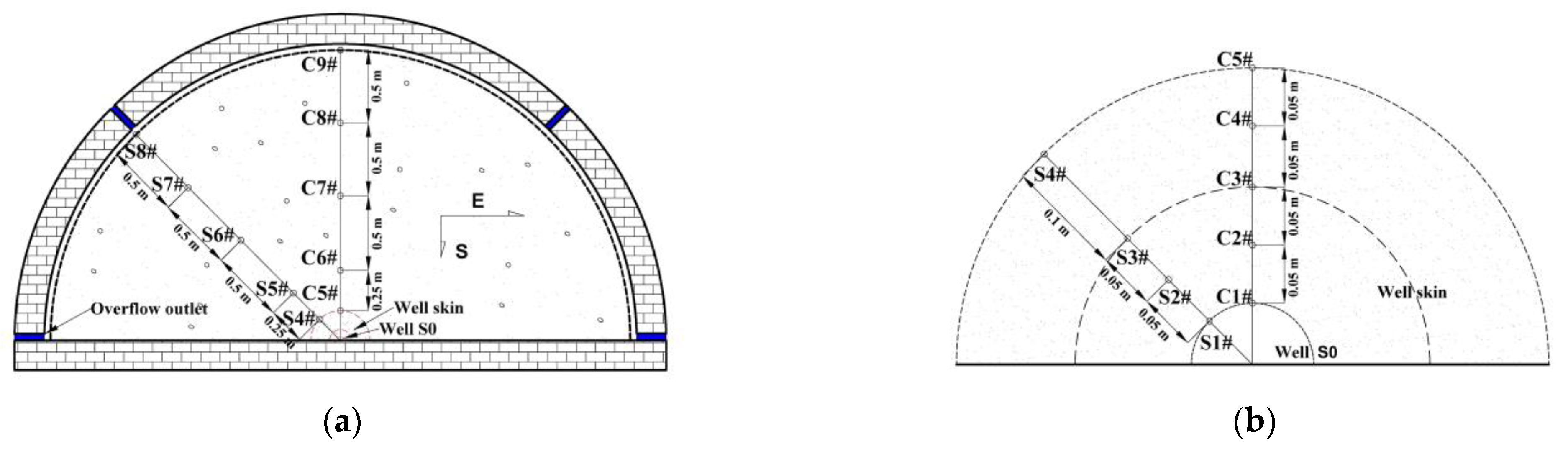
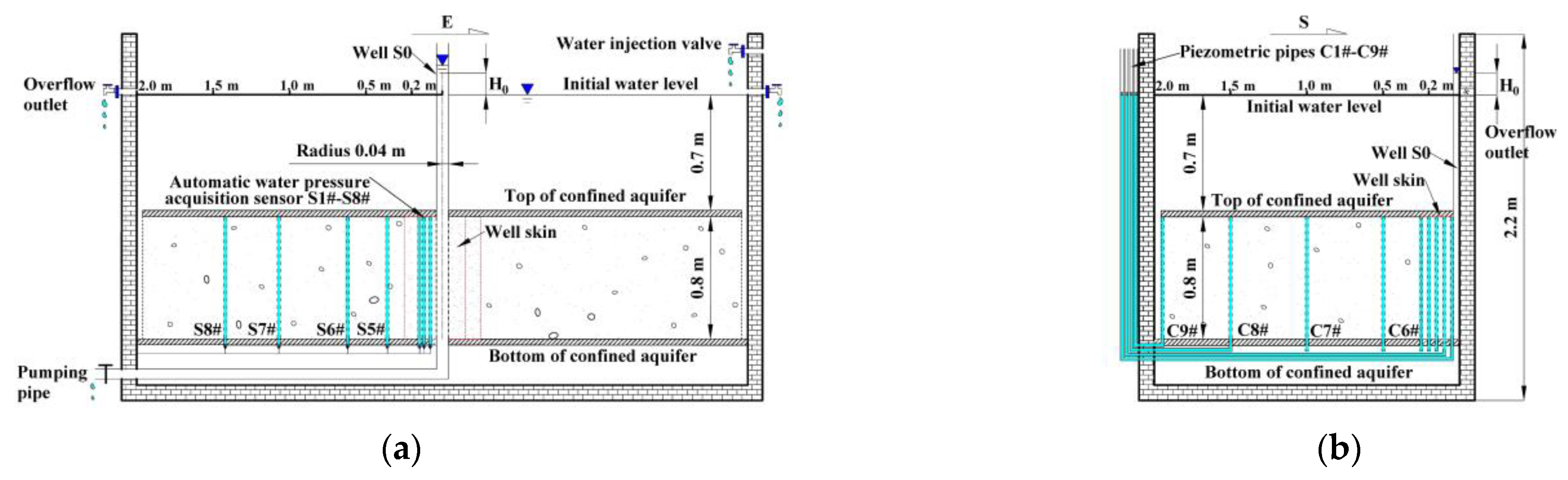
3. Indoor Model Tests

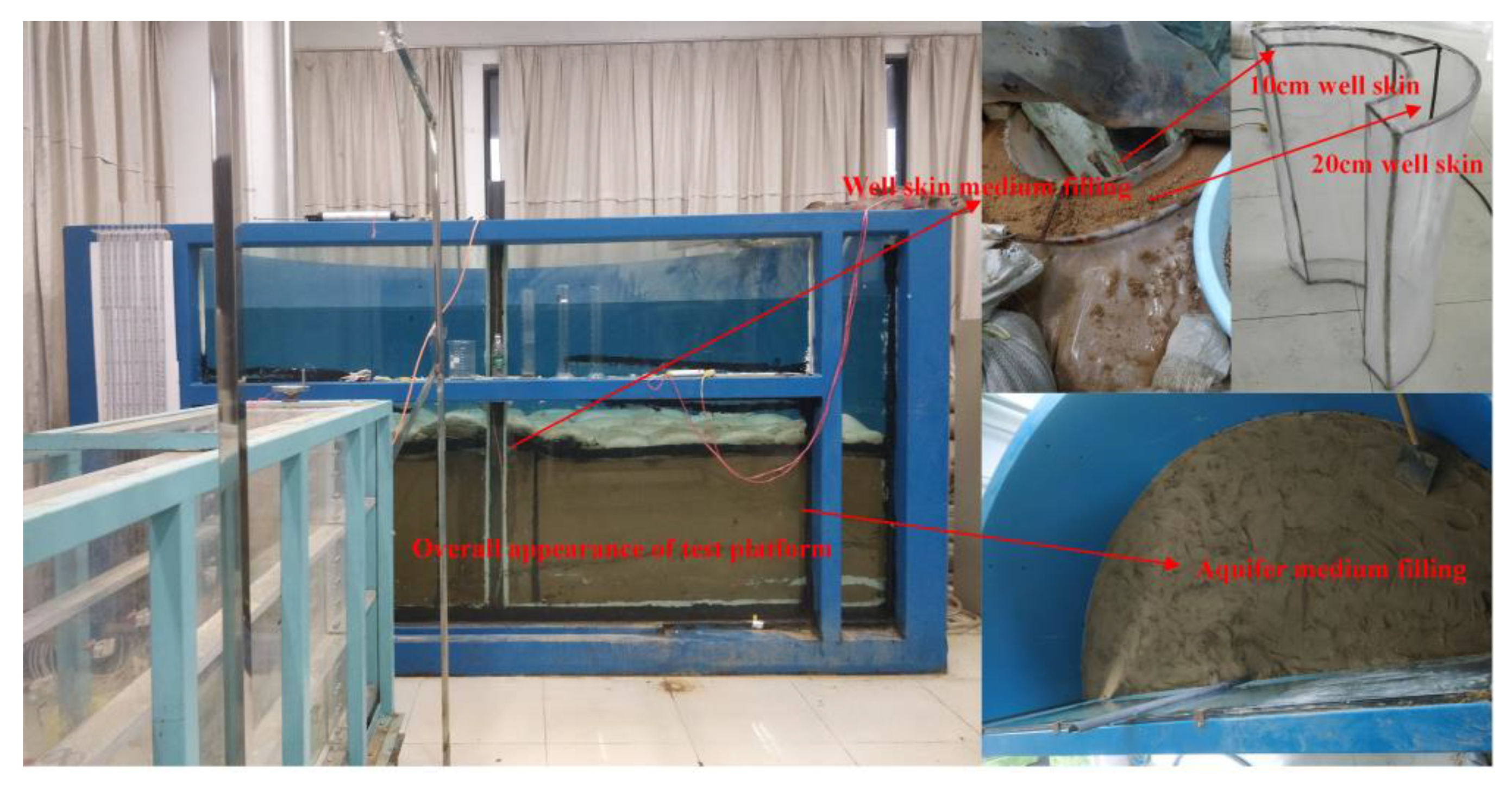
3.1. Test Platform Construction

(1) Aquifer System
Based on the assumptions of the radial flow and the principle of axisymmetry in the groundwater well flow problem, a semi-circular model in the axisymmetric model was utilized for the test platform to save test space. The overall design of the model is a 2.2 m high, 2 m radius semi-cylindrical sand tank with a test well in the centre of the semi-cylindrical section. The test well has an internal diameter of 0.08 m and an external diameter of 0.10 m. Overflow outlets are uniformly arranged at the upper 1.5 m of the model bottom plate on the side of the semi-cylindrical arc to ensure that the boundary is a constant water head boundary during the test. The aquifer system simulates a confined aquifer with a thickness of 0.8 m. The aquifer medium is medium and fine sand with a particle size of 0.25 mm–0.50 mm. Both the top and bottom plates are provided with waterproof layers. A layer of sandbags is laid on the top of the top plate to apply pressure to simulate a confined aquifer. In addition, a gap is left at the circular boundary as a constant water head recharge boundary. As the research focuses on the influence of well-skin on this slug test, the setting of the well-skin layer is very important and two different thicknesses of well-skin layers were used to investigate the influence of different thicknesses of well-skin layer on the results of the slug test. The well-skin layer is located within 20 cm around the test well and is separated from the aquifer using a semi-cylindrical frame, which is divided into two semi-cylindrical zones of 0–10 cm and 10–20 cm. The positive well-skin is filled with a 1:1 mixture of silty clay and silty fine sand. When the well-skin is not set, the well-skin layer is filled with the same particle size of 0.25 mm–0.50 mm sand as the aquifer. The planar graph of the test platform model is shown in Figure 3, where Figure 3a shows the overall planar graph, and Figure 3b shows the local well-skin layer planar graph. The east–west section of the indoor test platform is shown in Figure 4a, and the north–south section is shown in Figure 4b. A physical picture of the indoor test platform is shown in Figure 5.
(2) Observation System
In order to ensure the reliability of the observation data, the observation system uses both piezometric pipes and automatic water pressure acquisition sensor. The main function of this system is to observe the change of water level data in real time during the test. The test well S0 is set in the centre of the semi-cylindrical section as part of both the piezometric pipe observation device and the automatic water pressure acquisition sensor device, and the piezometric pipes and automatic water pressure acquisition sensors are distributed in two radial directions of the semi-circular base plate.
The piezometric pipe observation device consists of the test well S0 and piezometric pipes C1#–C9#, which are, respectively, 0.05 m, 0.10 m, 0.15 m, 0.20 m, 0.25 m, 0.50 m, 1.00 m, 1.50 m, and 2.00 m away from the test well. The automatic water pressure acquisition sensor device consists of the test well S0 and observation holes S1#–S8#, which are, respectively, 0.05 m, 0.10 m, 0.15 m, 0.25 m, 0.50 m, 1.00 m, 1.50 m, and 2.00 m away from the test well. An automatic water pressure acquisition sensor was put into the test well S0 from the wellhead to record the water level change of the test well. The overall setup of the observation system is shown in Figure 3.

3.2. Test Programme

(1) Test Programme Design
The slug test is a method to determine the hydrogeological parameters of an aquifer by means of the change law of well water level with time caused by the change of small amount of water in the test well. For this indoor slug test, three different volumes of water lifting columns were used as excitation devices to meet the requirements of different excitation strengths: small (500 cm3), medium (1000 cm3), and large (1500 cm3) to meet the instantaneous characteristic of the water volume changes in the test well. In addition, to eliminate the possible influence of factors such as positive well-skin layer thickness and excitation strength, the indoor test programme was divided into three different well-skin conditions: no well-skin, 10 cm thick positive well-skin layer, and 20 cm thick positive well-skin layer. Three different excitation strengths for the water lifting slug test and three different pumping flow rates for large, medium, and small flow rates pumping test were conducted under different well-skin conditions. To avoid accidental errors, three parallel sets of tests were conducted simultaneously for each test. The pumping test and slug test numbers for each group are shown in Table 1.
(2) Test Steps and Methods
Before the start of the test, water was injected into the aquifer from the side of the model arc to saturate it layer by layer, with the air in the sand body drained outward. Water injection was stopped when the water level in the model completely immersed the aquifer sand body. The sand body was considered reaching saturation when the readings of each piezometric pipe and automatic water pressure acquisition sensor were basically the same and remained unchanged for a long time. Then, water was injected continuously until the water level reached the overflow outlets of the model, and there was water overflow. The pumping test and slug test were carried out after the water level in the model was always at the overflow outlets position, and the readings of each piezometric pipe and automatic water pressure acquisition sensor were stable and remained unchanged for a long time.

4. Test Results and Analysis

4.1. Pumping Test Method

The results of the pumping tests were processed and calculated using the Dupuit equation method [31] and the Thiem equation method [31]. The average value of the results of the two calculation methods for each group of pumping tests without well-skin model conditions was used as the reference value to verify the reliability and accuracy of the proposed theory and method (HWS model) for determining the aquifer permeability coefficient by slug tests under the positive well-skin effect. The results of the permeability coefficients calculated by the pumping test method without well-skin model conditions are shown in Table 2.
By comparing the mean values of the results calculated by the two methods in Table 2, they are basically consistent, indicating a reasonable test design. Therefore, the average value of the aquifer permeability coefficient calculated under both methods was used as the reference value of the aquifer permeability coefficient determined by the pumping tests without well-skin conditions.
After setting up the positive well-skin layer, the pumping test observation data from the positive well-skin layer and the aquifer were calculated using the Theim equation method to obtain the reference value of the permeability coefficient of the positive well-skin layer. The calculation results obtained are shown in Table 3.
As shown in Table 3, the aquifer permeability coefficient determined from pumping tests became significantly smaller after the installation of the positive well-skin layer. In the case of the 20 cm thick well-skin, the permeability coefficient of the aquifer determined from pumping tests was even smaller due to the smaller permeability coefficient of the well-skin layer, indicating that the presence of the positive well-skin layer had a great impact on the aquifer permeability coefficient determined from pumping tests.
However, the permeability coefficient of the positive well-skin layer can be accurately obtained by using the observation data in the positive well-skin layer. Therefore, the calculation results of the observation data in the positive well-skin layer using Theim’s equation method show that the reference values of the permeability coefficient in the positive well-skin layer as ρ s = 3.75 and ρ s = 6.25 are 0.0276 cm·s−1 and 0.0172 cm·s−1, respectively.

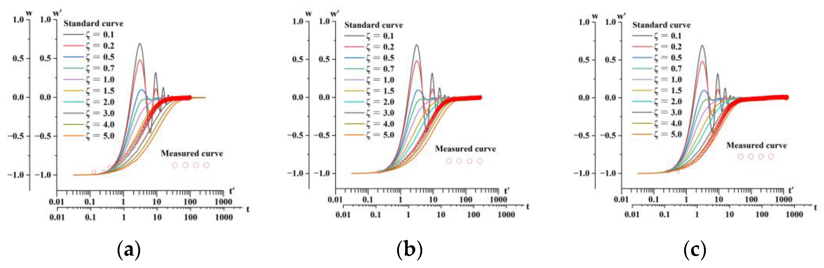
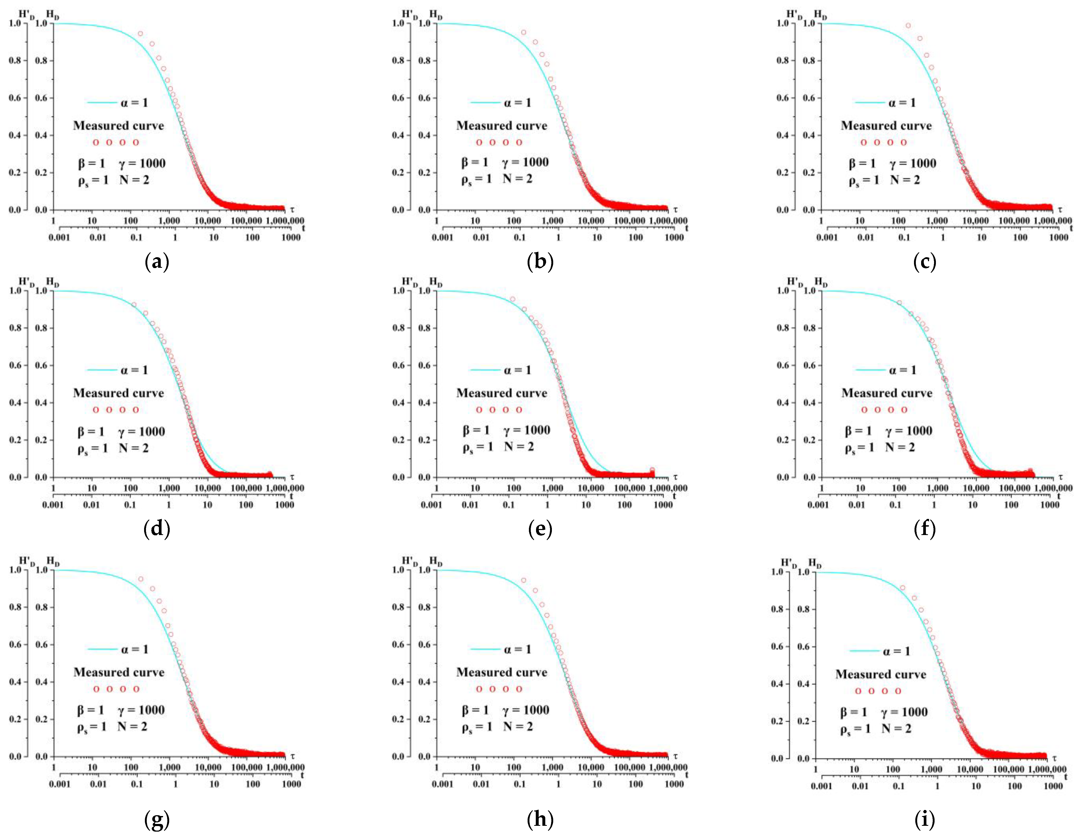
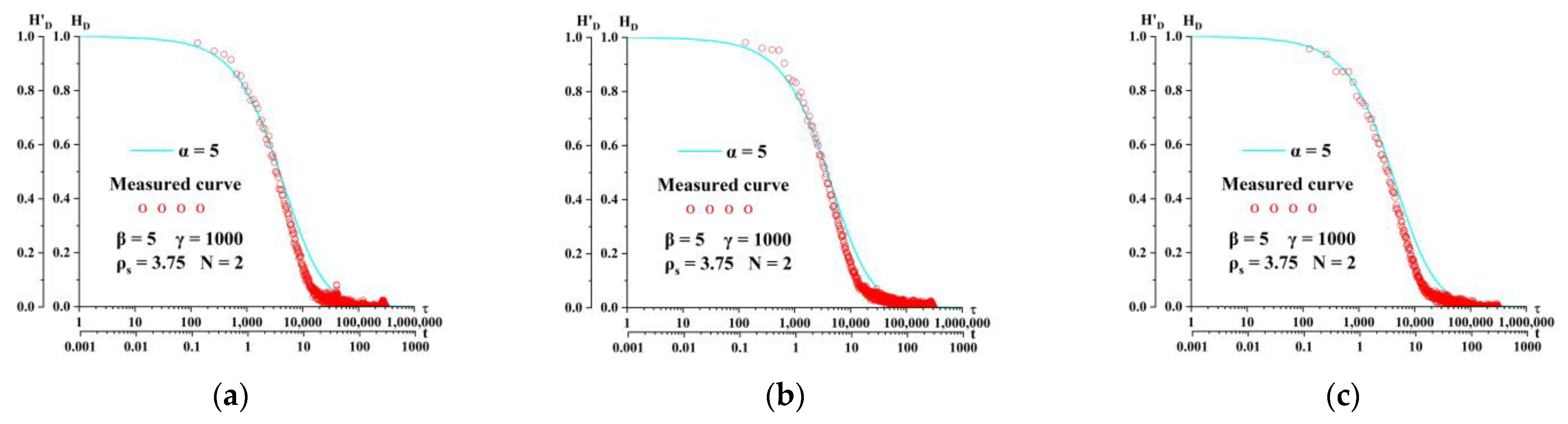
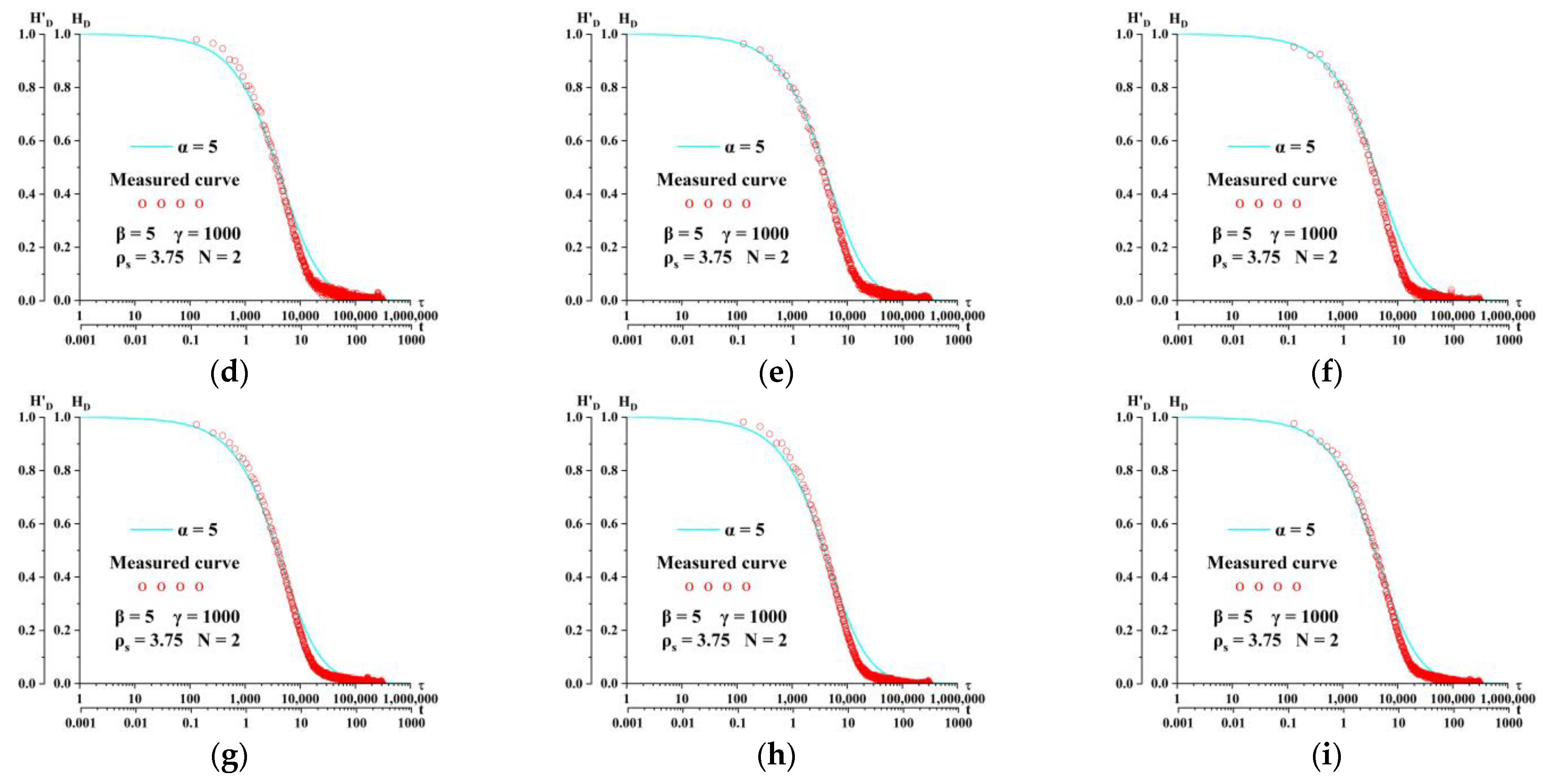
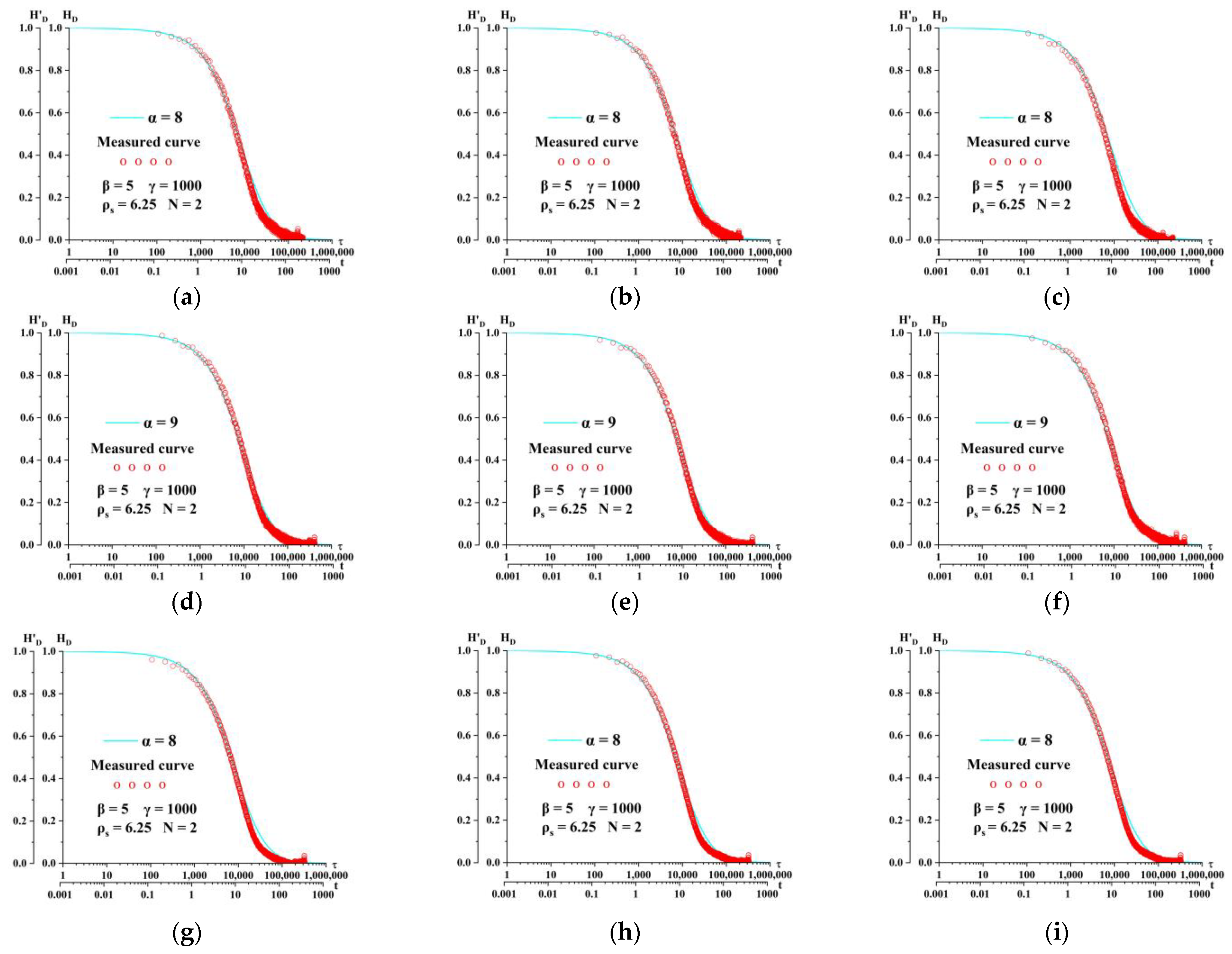
4.2. Slug Test Method

The slug test data were analysed and calculated with the Kipp model and the proposed theoretical model for slug test under positive well-skin effect (HWS model), respectively.
(1) Kipp model analysis method [5] (without considering the well-skin effect model)
The Kipp model uses dimensionless factors and parameter variables to convert the differential equation of water flow oscillations within a single well into dimensionless form and obtain a set of standard curves. The test data were processed, and the permeability coefficient values were solved using the matching method, and the partial Kipp model matching fitting diagram without well-skin model conditions are shown in Figure 6, and the final calculation results are shown in Table 4.
From Table 4, the average values of the permeability coefficients calculated from the slug tests with different excitation strengths under the no well-skin model conditions are in general agreement with the reference values of the permeability coefficients calculated from the conventional pumping tests. This indicates that accurate results can be obtained from the slug test data using the Kipp model under the no well-skin model conditions. However, the calculated values based on the Kipp model under positive well-skin model conditions are between the aquifer permeability coefficient and the positive well-skin layer permeability coefficient, which represents the average value of the positive well-skin layer and aquifer permeability coefficient under the influence of positive well-skin. This implies that the slug test is influenced by positive well-skin, and the Kipp model is no longer applicable to the slug test under positive well-skin model conditions.
(2) Analytical approach to the theoretical model of the slug test under positive well-skin effect (HWS model)
According to the well-skin layer model conditions of the indoor test, standard curves were plotted for no well-skin ( ρ s = 1, β = 1, γ = 1000), 10 cm thick positive well-skin layer ( ρ s = 3.75, β = 5, γ = 1000), and 20 cm thick positive well-skin layer ( ρ s = 6.25, β = 5, γ = 1000), respectively. We next took the test data of H D and time t in the slug test under different well-skin model conditions and drew a single logarithmic relationship curve, fitted it with the standard curve (Figure 7, Figure 8 and Figure 9), chose any matching point, and recorded the coordinate values of [ τ ] and [ t ] corresponding to the standard curve and the measured curve, and then the aquifer permeability coefficient K 2 could be obtained. Then, based on the value of α , the well-skin layer permeability coefficient K 1 could be obtained.
The HWS model was used to analyze the test data of each group. The calculation results of the aquifer and well-skin layer permeability coefficients were obtained, respectively, and shown in Table 5.

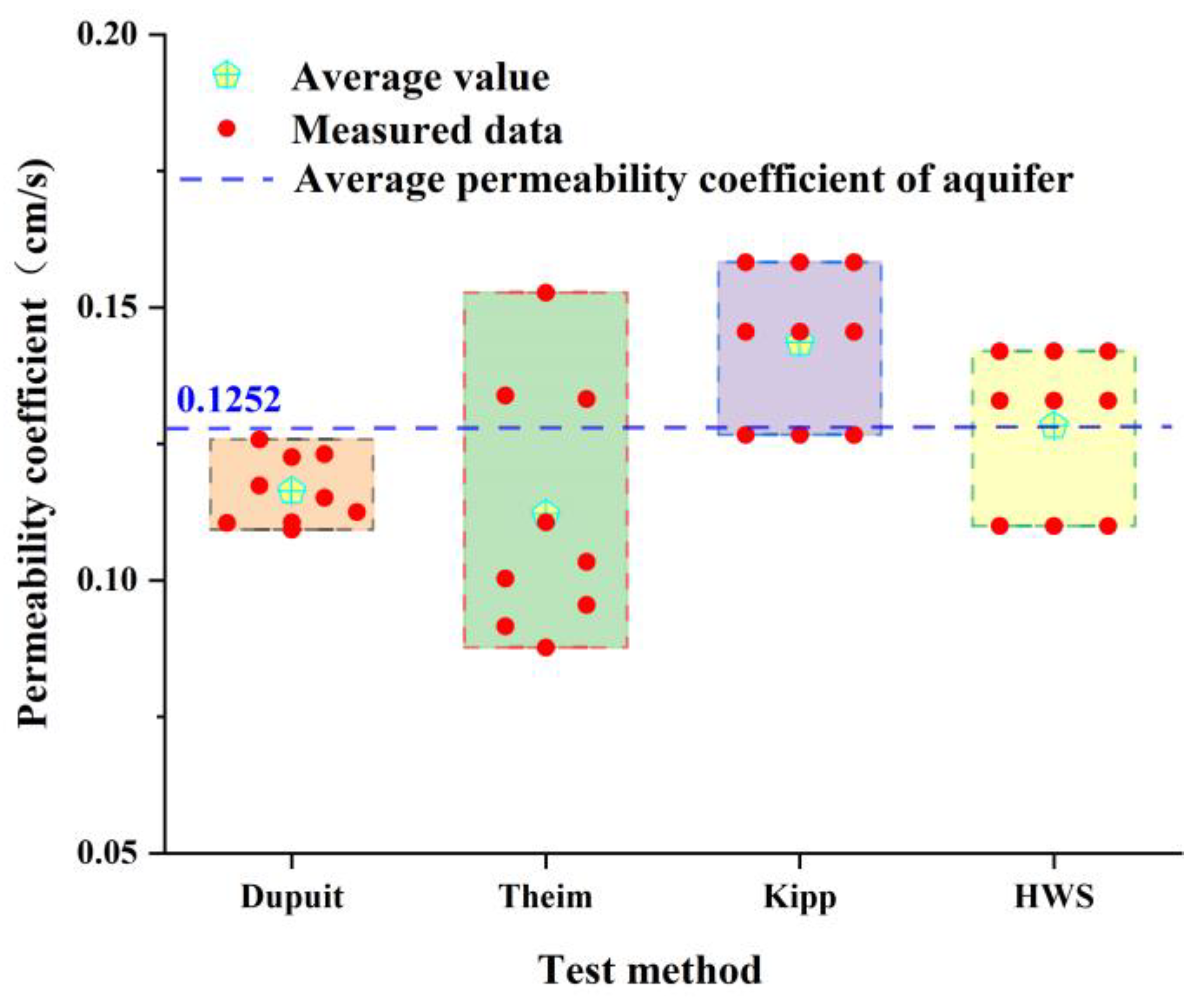
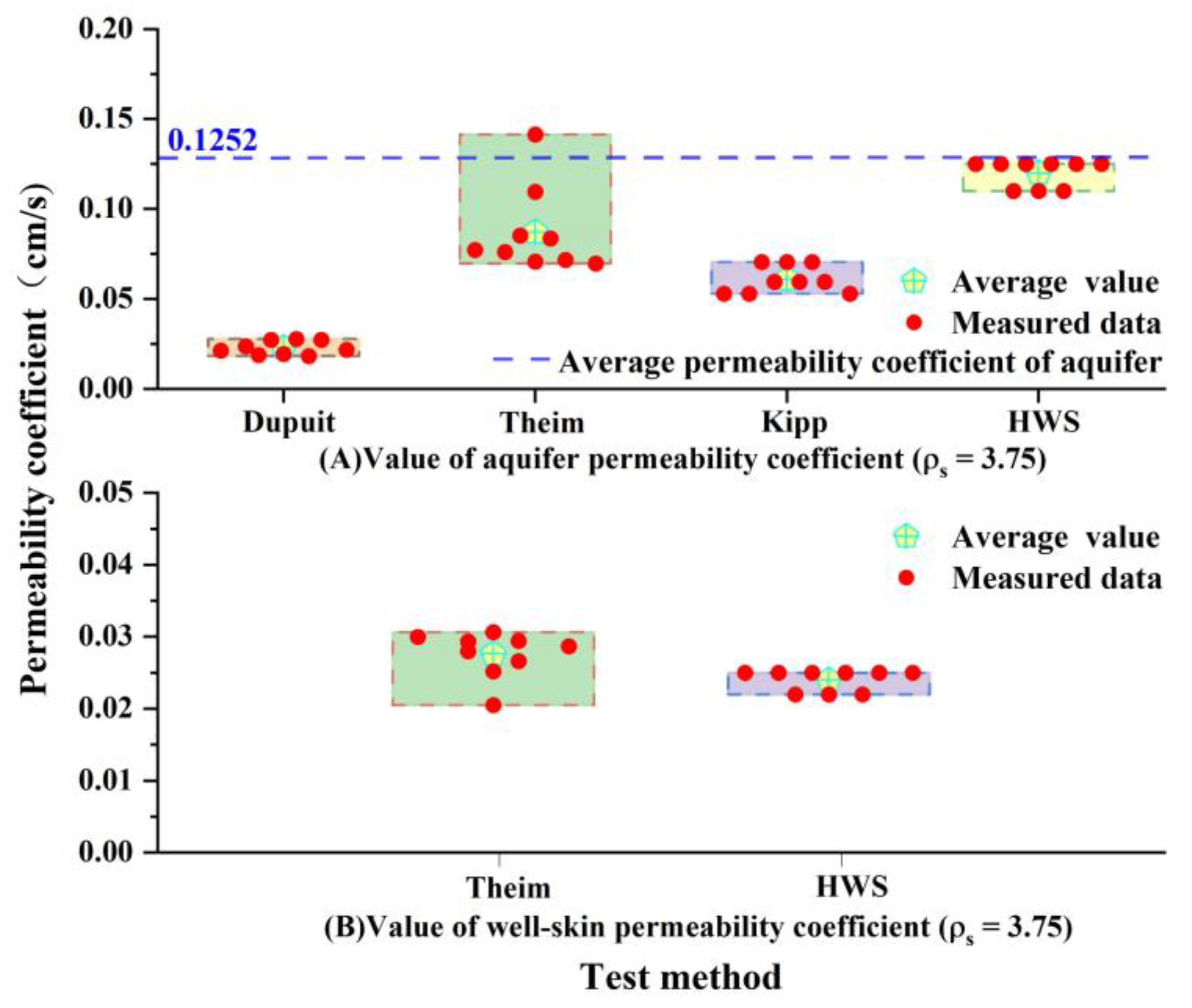
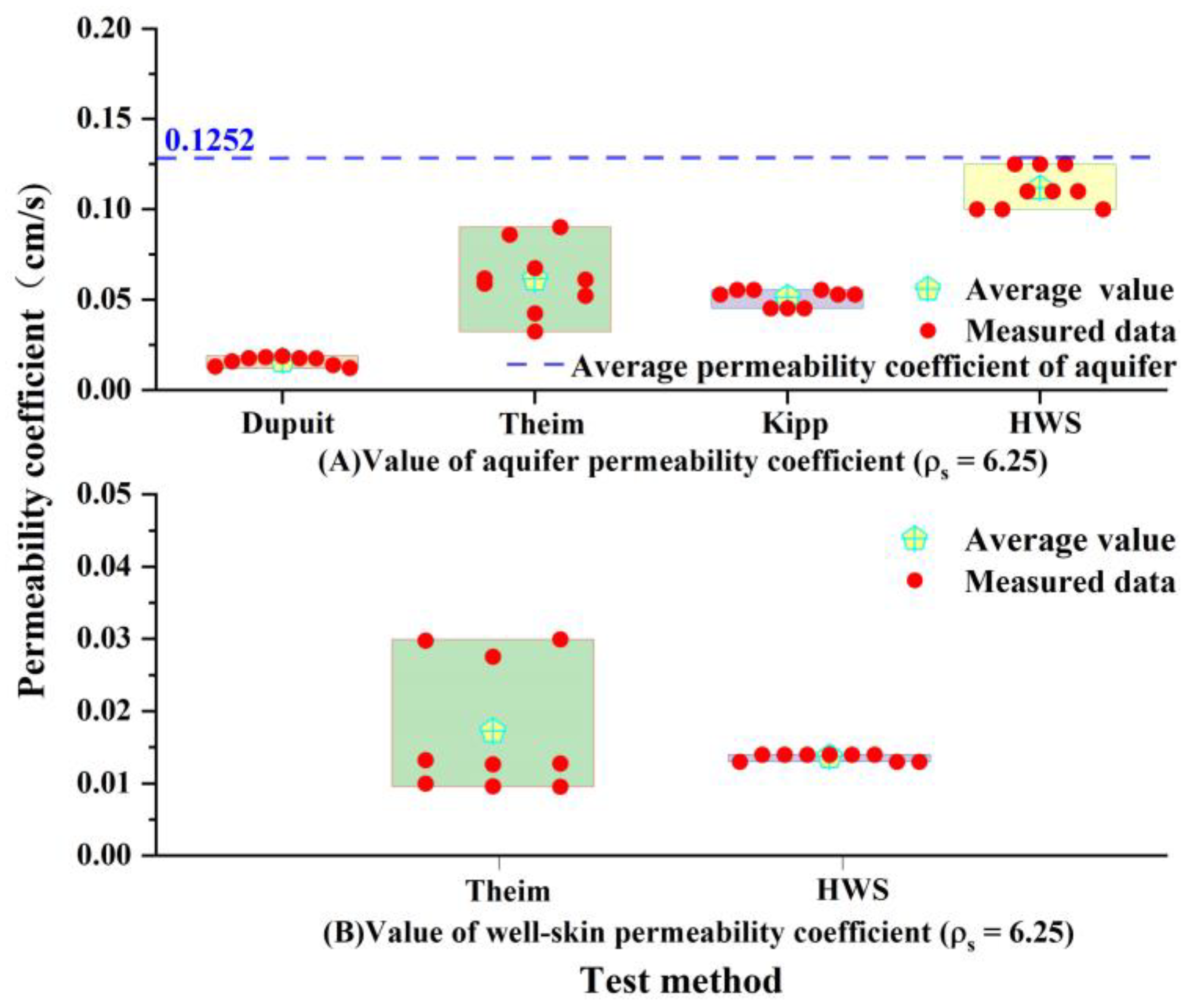
4.3. Comparison and Analysis of Calculation Results

Based on the calculation results in Table 2, Table 3, Table 4 and Table 5, the permeability coefficients of aquifer and well-skin layers in different well-skin conditions obtained by different calculation methods were compared and analysed as shown in Figure 10, Figure 11 and Figure 12.
The average value of the Dupuit equation method, Theim equation method, Kipp model, and HWS model was used as the reference value of aquifer permeability coefficient (0.1252 cm·s−1) under the no well-skin model conditions. The calculation results of different test methods show that the calculation results of Kipp model of the slug test are generally larger than the reference value, and the calculation results of HWS model are more similar to the reference value; that is, the HWS model can obtain accurate aquifer permeability coefficient values based on the slug test data under the no well-skin model. Meanwhile, it can be seen from Figure 10 that the calculation results based on the slug test are more stable under the same excitation strength.
Comparing the results of the different analytical methods for ρ s = 3.75 (10 cm thick positive well-skin layer), both the pumping test and the slug test Kipp model analytical methods are affected by the positive well-skin effect in the calculation of the aquifer permeability coefficient, resulting in small results. The HWS model overcomes the influence of the positive well-skin effect. The average value (0.1200 cm·s−1) of the HWS model is in good agreement with the reference value (0.1252 cm·s−1) of permeability coefficient. Meanwhile, the average value (0.0240 cm·s−1) of the permeability coefficient of the positive well-skin layer calculated by the HWS model is consistent with the average value (0.0276 cm·s−1) of the permeability coefficient of the positive well-skin layer calculated using the Theim equation method based on the observation test data within the positive well-skin layer. This shows that the permeability coefficient obtained from the HWS model for ρ s = 3.75 is accurate under positive well-skin effect.
Comparing the results obtained by different analytical method for ρ s = 6.25 (20 cm thick positive well-skin layer), it can be seen that as the thickness of the well-skin layer becomes larger, the positive well-skin effect has a greater impact on the calculation results of the pumping test. Compared to the pumping test and the Kipp model of the slug test, the average value (0.1120 cm·s−1) of the aquifer permeability coefficient calculated by the HWS model for ρ s = 6.25 is essentially the same as the reference value of aquifer permeability coefficient (0.1252 cm·s−1) under the no well-skin model conditions. The calculation results of the permeability coefficient of the positive well-skin layer for ρ s = 6.25 of both the pumping test Theim equation method and the HWS model are smaller than those for ρ s = 3.75, probably because the thickening of the positive well-skin layer makes the filling medium more compact and leads to a smaller permeability coefficient value. The average value (0.0140 cm·s−1) calculated by the HWS model for the positive well-skin layer of ρ s = 6.25 is similar to the average value (0.0172 cm·s−1) of the permeability coefficient of the positive well-skin layer calculated using the Theim equation method based on the observation test data within the positive well-skin layer, indicating that the HWS model still maintains a high accuracy in calculating the permeability coefficient values for the aquifer and the positive well-skin layer at ρ s = 6.25.
Comparing the calculations results of aquifer permeability coefficient under different well-skin conditions, the Dupuit equation method of pumping test is more influenced by the positive well-skin effect, as the results obtained when using the test well for calculations represent the average permeability coefficient of the whole aquifer (including positive well-skin layer). Under the positive well-skin effect, the Theim equation method can obtain accurate values of the permeability coefficient of the positive well-skin layer based on the observation test data of the pumping test within the positive well-skin layer, but the calculated permeability value of the aquifer is greatly affected by the positive well-skin effect, and the calculation result is smaller. Compared to the Kipp model, which is only applicable to the no well-skin model conditions, the HWS model is applicable to various positive well-skin models and can accurately obtain the permeability coefficients of aquifer under various positive well-skin model conditions. The permeability coefficient of the positive well-skin layer calculated by the HWS model is similar to the value calculated by the Theim equation based on the observations test data of the pumping test within the positive well-skin layer. This implies that HWS model is accurate in the application of determining the permeability coefficient of aquifer using slug test data, and the HWS model can calculate the permeability coefficient value of the positive well-skin layer when the positive well-skin effect exists. Compared with the traditional pumping test method and Kipp model method of slug test, HWS model is more accurate in determining the aquifer permeability coefficient.
The proposed slug test theoretical model under the influence of positive well-skin effect was verified and compared in indoor finite scale model. Therefore, the application of the proposed theoretical model and method in the field test will be the focus of future research work. In the field application, it is necessary to consider the influence of scale effect, different excitation strength, and different excitation modes (water injection mode, water lift mode, and air pressure mode, etc.) on the test results.

5. Conclusions

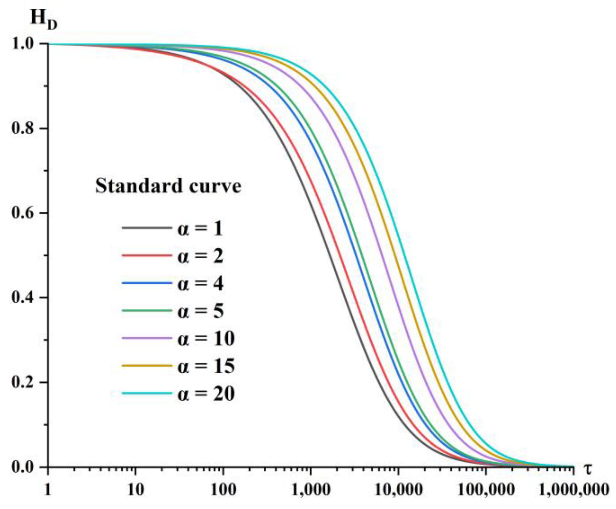
  • The theoretical model of the slug test considering the positive well-skin effect was solved by using the Laplace transform method and the AWG algorithm. Furthermore, multiple sets of standard curves under different well-skin conditions were plotted, and the specific parameter calculation methods and steps of the HWS model were proposed.
  • The presence of the positive well-skin layer had a great impact on the aquifer permeability coefficient determined from both pumping test and slug test, resulting in smaller results. The Kipp model is no longer applicable to the slug test under the influence of positive well-skin effect. The HWS model can overcome the influence of the positive well-skin effect, and the HWS model is applicable to the various positive well-skin models and the no well-skin model. When the positive well-skin effect exists, the HWS model can calculate not only the permeability coefficient of aquifers but also the permeability coefficient of the positive well-skin layer.
  • Multiple groups of standard curves under different well-skin conditions have obvious curve characteristics, and different standard curves have a high degree of discrimination. Therefore, by analysing the curve shape and characteristics of the HWS model, according to the different degree of the positive well-skin effect, it can be judged in the field test whether the positive well-skin effect exists based on the preliminary understanding of formation lithology.

Author Contributions

Conceptualization, Y.Z.; methodology, Y.Z.; validation, H.W., P.L. and X.D.; formal analysis, Y.Z., H.W., P.L. and X.D.; resources, Y.Z.; data curation, P.L. and X.D.; writing—original draft preparation, Y.Z.; writing—review and editing, H.W., X.D. and Y.Y.; visualization, H.W. and X.D.; supervision, Y.Z., Y.H. and J.W.; project administration, Y.Z., Y.H. and J.W.; funding acquisition, Y.Z. All authors have read and agreed to the published version of the manuscript.

Funding

This research was funded by the National Key Research and Development Program of China, grant number 2019YFC1510802, the Fundamental Research Funds for the Central Universities, grant number B220205006, and the scientific research project of water conveyance and irrigation project of Xixiayuan water control project in Henan Province, China, grant number XXYSS/GQ-KYXM-02.

Data Availability Statement

Not applicable.

Acknowledgments

The authors would like to thank the School of Earth Sciences and Engineering at Hohai University for partial support of the graduate student on this project.

Conflicts of Interest

The authors declare no conflict of interest.

References

  1. Xu, Q. Application analysis of hydrogeological slug test technology. China Urban Econ. 2010, 132–136. [Google Scholar]
  2. Hvorslev, M.J. Time Lag and Soil Permeability in Ground-Water Observations. US Army Bull. 1951, 36, 49. [Google Scholar]
  3. Cooper, H.H., Jr.; Bredehoeft, J.D.; Papadopulos, I.S. Response of a finite-diameter well to an instantaneous charge of water. Water Resour. Res. 1967, 3, 263–269. [Google Scholar] [CrossRef]
  4. Bouwer, H.; Rice, R.C. A slug test for determining hydraulic conductivity of unconfined aquifers with completely or partially penetrating wells. Water Resour. Res. 1976, 12, 423–428. [Google Scholar] [CrossRef] [Green Version]
  5. Kipp, K.L., Jr. Type Curve Analysis of Inertial Effects in the Response of a Well to a Slug Test. Water Resour. Res. 1985, 21, 1397–1408. [Google Scholar] [CrossRef]
  6. McElwee, C.D. Improving the analysis of slug tests. J. Hydrol. 2002, 269, 122–133. [Google Scholar] [CrossRef]
  7. Yong, H.; Zhifang, Z.; Jinguo, W. Method for determination of hydro-geological parameter of aquifers with low permeability and its application. J. Hohai Univ. Nat. Sci. 2006, 34, 672–675. [Google Scholar] [CrossRef]
  8. Zhou, Z.; Wang, Z.; Zeng, X.; Yang, J.; Chen, W. Development of rapid field test system for determining permeable parameters of rock and soil masses. Yanshilixue Yu Gongcheng Xuebao/Chin. J. Rock Mech. Eng. 2008, 27, 1292–1296. [Google Scholar]
  9. Zhao, Y.; Zhang, Z.; Rong, R.; Dong, X.; Wang, J. A new calculation method for hydrogeological parameters from unsteady-flow pumping tests with a circular constant water-head boundary of finite scale. Q. J. Eng. Geol. Hydrogeol. 2022, 55, qjegh2021-112. [Google Scholar] [CrossRef]
  10. Zhao, Y.; Zhou, Z. Comparative study on field slug tests to determine aquifer permeability based on Kipp model and CBP model. Geotech. Investig. Surv. 2012, 40, 32–38. [Google Scholar]
  11. Zhao, Y.-r.; Zhou, Z.-f. A field test data research based on a new hydraulic parameters quick test technology. J. Hydrodyn. 2010, 22, 562–571. [Google Scholar] [CrossRef]
  12. Liang, X.; Zhan, H.; Zhang, Y.-K.; Liu, J. Underdamped slug tests with unsaturated-saturated flows by considering effects of wellbore skins. Hydrol. Processes 2018, 32, 968–980. [Google Scholar] [CrossRef]
  13. Ramey, H.J.; Agarwal, R.G. Annulus Unloading Rates as Influenced by Wellbore Storage and Skin Effect. Soc. Pet. Eng. J. 1972, 12, 453–462. [Google Scholar] [CrossRef]
  14. Faust, C.R.; Mercer, J.W. Evaluation of Slug Tests in Wells Containing a Finite-Thickness Skin. Water Resour. Res. 1984, 20, 504–506. [Google Scholar] [CrossRef]
  15. Moench, A.F.; Hsieh, P.A. Comment on “Evaluation of Slug Tests in Wells Containing a Finite-Thickness Skin” by C. R. Faust and J. W. Mercer. Water Resour. Res. 1985, 21, 1459–1461. [Google Scholar] [CrossRef]
  16. Sageev, A. Slug Test Analysis. Water Resour. Res. 1986, 22, 1323–1333. [Google Scholar] [CrossRef]
  17. Mingyi, S.; Jiaxun, C. Slug test analysis of unconfined aquifers considering well skin effect. National PingTung University of Science and Technology. In Proceedings of the Forth Conference on Groundwater Resources and Water Quality Protection, Neipu, Taiwan, 14 April 2001. [Google Scholar]
  18. Tzeng, C. Method for Extrapolation of Experimental Parameters for Slug Test Affected by Negative Well Skin Effect. Natl. Cent. Univ. 2002. Available online: http://ir.lib.ncu.edu.tw:88/thesis/view_etd.asp?URN=89624004 (accessed on 20 September 2022).
  19. Rovey, C.W.; Niemann, W.L. Wellskins and slug tests: Where’s the bias? J. Hydrol. 2001, 243, 120–132. [Google Scholar] [CrossRef]
  20. Barrash, W.; Clemo, T.; Fox, J.J.; Johnson, T.C. Field, laboratory, and modeling investigation of the skin effect at wells with slotted casing, Boise Hydrogeophysical Research Site. J. Hydrol. 2006, 326, 181–198. [Google Scholar] [CrossRef]
  21. Yeh, H.-D.; Chen, Y.-J. Determination of skin and aquifer parameters for a slug test with wellbore-skin effect. J. Hydrol. 2007, 342, 283–294. [Google Scholar] [CrossRef]
  22. Chen, Z.; Yuan, G.; Zhao, B. A study on application of slug test. Geotech. Investig. Surv. 2009, 37, 31–34. [Google Scholar] [CrossRef] [Green Version]
  23. Ju, X.; He, J.; Wang, J.; Ma, W.; Lu, Y. Comparison of the determination of hydrogeological parameters from pumping tests and slug tests. Geotech. Investig. Surv. 2011, 39, 51–56. [Google Scholar] [CrossRef] [Green Version]
  24. Cardiff, M.; Barrash, W.; Thoma, M.; Malama, B. Information content of slug tests for estimating hydraulic properties in realistic, high-conductivity aquifer scenarios. J. Hydrol. 2011, 403, 66–82. [Google Scholar] [CrossRef]
  25. Sahin, A.U. Simple methods for quick determination of aquifer parameters using slug tests. Hydrol. Res. 2017, 48, 326–339. [Google Scholar] [CrossRef]
  26. Weeks, E.P.; Clark, A.C. Evaluation of Near-Critical Overdamping Effects in Slug-Test Response. Ground Water 2013, 51, 775–780. [Google Scholar] [CrossRef]
  27. Liu, Q.; Hu, L.; Bayer, P.; Xing, Y.; Qiu, P.; Ptak, T.; Hu, R. A Numerical Study of Slug Tests in a Three-Dimensional Heterogeneous Porous Aquifer Considering Well Inertial Effects. Water Resour. Res. 2020, 56, e2020WR027155. [Google Scholar] [CrossRef]
  28. Morozov, P.E. Assessing the Hydraulic Conductivity Anisotropy and Skin-Effect Based on Data of Slug Tests in Partially Penetrating Wells. Water Resour. 2020, 47, 430–437. [Google Scholar] [CrossRef]
  29. Stehfest, H. Numerical Inversion of Laplace Transforms. Commun. ACM 1970, 13, 624. [Google Scholar] [CrossRef]
  30. He, G.Y.; Li, L. An application of AWG method of numerical inversion of Laplace transform for flow in a fluid finite-conductivity vertical fractures. Pet. Explor. Dev. 1995, 22, 47–50. [Google Scholar]
  31. Zhifang, Z.; Jinguo, W. Groundwater Dynamics, 1st ed.; Science Press: Beijing, China, 2013. [Google Scholar]
Figure 1. Schematic diagram of the slug test model considering well-skin effect (The red dashed line represents the outer wall of the well skin layer, and the red area represents the internal structure of the well skin layer).
Water 14 03089 g001
Figure 2. HWS model standard curve.
Water 14 03089 g002
Figure 3. Indoor test platform planar graph. (a) Whole planar graph. (b) Well-skin planar graph.
Water 14 03089 g003
Figure 4. Section of indoor test platform. (a) East–West Section. (b) South–North Section.
Water 14 03089 g004
Figure 5. Physical picture of indoor test platform.
Water 14 03089 g005
Figure 6. Partial slug test Kipp model matching fitting diagram under none well-skin model conditions. (a) N-Sls2. (b) N-Slm2. (c) N-Sll3.
Water 14 03089 g006
Figure 7. Curve fitting diagram between measured data from slug test and HWS model standard curve under the no well-skin conditions. (a) N-Sls1. (b) N-Sls2. (c) N-Sls3. (d) N-Slm1. (e) N-Slm2. (g) N-Sll1. (h) N-Sll2. (i) N-Sll3.
Water 14 03089 g007
Figure 8. Curve fitting diagram between measured data from slug test and HWS model standard curve under model conditions of ρ s = 3.75. (a) P10-Sls1. (b) P10-Sls2. (c) P10-Sls3. (d) P10-Slm1. (e) P10-Slm2. (f) P10-Slm3. (g) P10-Sll1. (h) P10-Sll2. (i) P10-Sll3.
Water 14 03089 g008aWater 14 03089 g008b
Figure 9. Curve fitting diagram between measured data from slug test and HWS model standard curve under model conditions of ρ s = 6.25. (a) P20-Sls1. (b) P20-Sls2. (c) P20-Sls3. (d) P20-Slm1. (e) P20-Slm2. (f) P20-Slm3. (g) P20-Sll1. (h) P20-Sll2. (i) P20-Sll3.
Water 14 03089 g009
Figure 10. Calculation results of permeability coefficients of aquifer for each analytical method under the no well-skin conditions (The different colour blocks represent the calculated value range of permeability coefficient under different methods).
Water 14 03089 g010
Figure 11. Calculation results of permeability coefficients of aquifer and well-skin layers for each analytical method for ρ s = 3.75 (10 cm thick positive well-skin layer) (The different colour blocks represent the calculated value range of permeability coefficient under different methods).
Water 14 03089 g011
Figure 12. Calculation results of permeability coefficients of aquifer and well-skin layers for each analytical method for ρ s = 6.25 (20 cm thick positive well-skin layer) (The different colour blocks represent the calculated value range of permeability coefficient under different methods).
Water 14 03089 g012
Table 1. Table of test numbers.
Pumping Flow Rate
(Q/m3·d−1)
Pumping Test Method
No Well-Skin10 cm Thick Positive Well-Skin Layer20 cm Thick Positive Well-Skin Layer
ρ s = 3.75 ρ s = 6.25
Small flow rate
(12.4416 m3·d−1)
N-Ps1P10-Ps1P20-Ps1
N-Ps2P10-Ps2P20-Ps2
N-Ps3P10-Ps3P20-Ps3
Medium flow rate (17.4528 m3·d−1)N-Pm1P10-Pm1P20-Pm1
N-Pm2P10-Pm2P20-Pm2
N-Pm3P10-Pm3P20-Pm3
Large flow rate
(23.3280 m3·d−1)
N-Pl1P10-Pl1P20-Pl1
N-Pl2P10-Pl2P20-Pl2
N-Pl3P10-Pl3P20-Pl3
Excitation strength Slug test method
No well-skin10 cm thick positive well-skin layer20 cm thick positive well-skin layer
ρ s = 3.75 ρ s = 6.25
Small column
(500 cm3)
N-Sls1P10-Sls1P20-Sls1
N-Sls2P10-Sls2P20-Sls2
N-Sls3P10-Sls3P20-Sls3
Medium column
(1000 cm3)
N-Slm1P10-Slm1P20-Slm1
N-Slm2P10-Slm2P20-Slm2
N-Slm3P10-Slm3P20-Slm3
Large column
(1500 cm3)
N-Sll1P10-Sll1P20-Sll1
N-Sll2P10-Sll2P20-Sll2
N-Sll3P10-Sll3P20-Sll3
Table 2. Calculated results of pumping tests to determine permeability coefficients under the no well-skin model conditions.
Test GroupDupuit Equation
K Avg./cm·s−1
Theim Equation
K Avg./cm·s−1
K Avg./cm·s−1
N-Ps1/2/30.12390.11970.1218
N-Pm1/2/30.11440.10950.1120
N-Pl1/2/30.11080.10740.1091
K Avg./cm·s−10.11640.11210.1143
Table 3. Calculation of results permeability coefficients determined by pumping tests under positive well-skin model conditions.
Test GroupDupuit Equation K Avg./cm·s−1Theim Equation K Avg./cm·s−1
Based on Test Well Test DataBased on Aquifer Observation DataBased on Positive Well-Skin Layer Observation Data
P10-Ps1/2/30.02740.09600.0250
P10-Pm1/2/30.02220.07750.0280
P10-Pl1/2/30.01880.08800.0298
K Avg./cm·s−10.02280.08720.0276
P20-Ps1/2/30.01820.05490.0166
P20-Pm1/2/30.01700.06270.0176
P20-Pl1/2/30.01300.06640.0174
K Avg./cm·s−10.01610.06130.0172
Table 4. Calculation results of permeability coefficients of the Kipp model in the slug test.
None Well-Skin ρ s = 3.75 ρ s = 6.25
Test GroupK Avg./cm·s−1Test GroupK Avg./cm·s−1Test GroupK Avg./cm·s−1
N-Sls1/2/30.1583P10-Sls1/2/30.0704P20-Sls1/2/30.0452
N-Slm1/2/30.1456P10-Slm1/2/30.0594P20-Slm1/2/30.0554
N-Sll1/2/30.1267P10-Sll1/2/30.0528P20-Sll1/2/30.0528
K Avg./cm·s−10.1435 0.0609 0.0511
Table 5. Calculation results of permeability coefficient determined by slug test based on HWS model under different well-skin effects.
Test Number α Aquifer Permeability Coefficient K2 Avg./cm·s−1
N-Sls1/2/310.1330
N-Slm1/2/310.1110
N-Sll1/2/310.1430
K Avg./cm·s−1 0.1290
Test number α Aquifer permeability coefficient
K2 Avg./cm·s−1
Positive well-skin layer permeability coefficient
K1 Avg./cm·s−1
P10-Sls1/2/350.12500.0250
P10-Slm1/2/350.12500.0250
P10-Sll1/2/350.11000.0220
K Avg./cm·s−10.12000.0240
P20-Sls1/2/380.11000.0140
P20-Slm1/2/390.12500.0140
P20-Sll1/2/380.10000.0130
K Avg./cm·s−10.11200.0140
Publisher’s Note: MDPI stays neutral with regard to jurisdictional claims in published maps and institutional affiliations.

