Mathematical Modeling-Based Management of a Sand Trap throughout Operational and Maintenance Periods (Case Study: Pengasih Irrigation Network, Indonesia)

Abstract

Surface irrigation networks in Indonesia are damaged by several factors, and sedimentation is among the most severe challenges. Sand traps play a substantial role in improving irrigation system efficiency by reducing sedimentation. There are two periods in sand trap operation: the operational and maintenance periods. Pengasih is one of the irrigation schemes implemented in the Progo Opak Serang (POS) River Basin, which has a high level of erosion. This study aimed to propose an appropriate management strategy for the Pengasih sand trap as the first barrier in irrigation network sedimentation based on mathematical modeling. The HEC-RAS simulation software was used to simulate the sand trap hydraulic behaviour. The results show that the validated Manning’s coefficient was 0.025. The optimal transport parameters were Laursen for the potential function, Exner 5 for the sorting method, and Rubey for the fall velocity method. The recommended flushing timeframe is 315 min, with a discharge of 2 m³/s. We suggest that the sand trap flushing frequency be performed twice a year, and it can be performed at the end of March and October. This coincides with the end of the first and third planting seasons of the irrigation scheme.

1. Introduction

Water resources have become the most vital element for human survival. Humans use water for numerous purposes, including agriculture, industry, housing, recreation, and the preservation of the environment [1]. Agricultural production consumes more fresh water than other human activity, estimated at approximately 70% [2,3,4]. Water resources for agriculture and food production are either classified as surface or ground water. In humid climates, surface water is the primary source of water for irrigation systems, while ground water is the main source of water in sub-humid and arid climates [5]. In places where expanding development necessitates agricultural expansion, irrigation water withdrawals are necessary [6,7,8]. Irrigation is the regulated artificial application of water to the soil to replace the water absorbed by crops [9]. Irrigation is essential for achieving food security as irrigated crops comprise 40% of global food production [10,11].

Indonesia is one of the few countries that have extensive technical irrigation infrastructure to store and distribute surface water to agricultural land. The irrigated area in Indonesia reaches around 7.3 million hectares, consisting of 48,000 schemes [12]. Based on the report from the Directorate General of Water Resources, in 2018 the Ministry of Public Works and Housing of the Republic of Indonesia reported that 46% of the surface irrigation network in Indonesia was damaged [13]. This damage was caused by several factors, including a lack of maintenance of the irrigation infrastructure services, poor management system, inappropriate rehabilitation system, and inadequate financing systems [14]. As it pertains to the irrigation infrastructure, the current deterioration is a result of an environment that significantly differs from the intended specifications. Sedimentation is one of the most significant infrastructure issues, from weirs to tertiary level irrigation channels [15,16]. Sedimentation in the irrigation infrastructure can be caused by excessive erosion in the weir upstream due to inadequate conservation of the river basin [16,17]. Sedimentation reduces the irrigation canal conveyance efficiency, leading to inadequacy and inequity in the water distribution to crops [18,19,20]. The government of Indonesia is implementing an irrigation modernization program to deal with multiple issues, including sedimentation. Irrigation modernization is an effort aimed at establishing a participatory irrigation management system capable of providing irrigation services in an effective, efficient, and sustainable manner [14,21,22].

The implementation of irrigation modernization is measured by several indicators, including increased water productivity, improved irrigation services, improved irrigation efficiency, increased financial sustainability, fewer disputes, and reduced environmental damage [21]. To deal with the indicator of improved irrigation efficiency, a sedimentation countermeasure is required. Sand traps are among the most effective devices for removing sediment particles from flowing water [23]. Sand traps play a significant role in preventing or minimizing the sedimentation in the canal and are generally used to improve irrigation system efficiency [24]. As shown in Figure 1, a sand trap is positioned directly downstream of the irrigation intake and is equipped with a flushing gate [15,25]. The function of this structure is to deposit the sediment entering the irrigation intake before it enters the primary irrigation channel [26]. Periodically, the sediment deposited in the sand trap is removed, either manually or hydraulically [15,23,24]. The effort spent on removing sediment from a sand trap is termed the maintenance/flushing period. The interval between the two flushing phases is regarded as the operational/settlement period. An effective sand trap is indicated by its capacity to hydraulically deposit and flush sediment during periodic flushing operations; It allows the sand trap to function effectively and sustainably [24,26].

The Progo Opak Serang (POS) River Basin in Indonesia is one of the river basins with a significant sedimentation potential [17]. The POS is a cross-provincial river basin covering a total area of 4994 km², including the Special Region of Yogyakarta (Daerah Istimewa Yogyakarta/DIY) and Central Java Province, and is governed by the Large River Basin Organization of Serayu Opak [17]. The POS River Basin plays a critical role in providing the water needs in the DIY and Central Java Province, one of which is the requirement of agricultural water, primarily supplied through surface irrigation networks. Concerning the POS River Basin’s potential for sedimentation, 38% of the basin’s area was designated as critical land, with an erosion rate of 235 tons/hectare/year [27]. The Pengasih irrigation scheme is one of the irrigation schemes included in the scope of the WS POS, with an area of 2291 ha. It receives its water supply from the Serang River through the Pengasih Weir. The Serang Watershed is one of the most critical potential watersheds from a landform and land use perspective [28,29]. The slope length and steepness (LS) and soil erodibility (K) have contributed most to the erosion in the Serang Watershed [28]. The high level of erosion in the Serang watershed causes high sedimentation in the Pengasih irrigation scheme. Sedimentation causes plenty of irrigation operation and maintenance (OM) problems. Vast amounts of money are required to maintain the networks, which is often an issue in developing countries, including Indonesia [30]. Therefore, this study aimed to propose an appropriate management strategy for the Pengasih sand trap as the first barrier in irrigation network sedimentation, both in the operational and maintenance periods, based on mathematical modeling. This study can be used as a reference in the guidelines for the operation and maintenance of the irrigation network.

2. Materials and Methods

2.1. Scope of Work

Pengasih is an irrigation scheme that draws the water from the Serang River [17,31]. The Serang Watershed, with the length of the main river reaching 28 km, is located in the Kulon Progo Regency, Special Region of Yogyakarta, Indonesia. In 2009, the Serang Watershed had a 9% critical land area, a slightly critical land area of 29%, a potentially crucial land area of 55%, and a non-critical land area of 7% [32]. This indicated that the Serang watershed was in a precarious state that could result in land degradation, erosion, and landslides [33,34,35]. In the Kulon Progo Regency area, the Sermo Reservoir is currently in operation and dams the Ngrancah River (a tributary of the Serang River) for the main purposes of irrigation and drinking water [27]. Pengasih is one of the irrigation schemes that receive an additional water supply from the Sermo Reservoir [31]. The Pengasih Weir, located at 7°50′08.88″ S and 110°10′16.73″ E, supplies 2077 hectares of paddy fields via an irrigation intake, primary irrigation channel, and nine secondary channels. The system is thus called the Pengasih irrigation scheme, and the location is shown in Figure 2. This study focused on the sand trap of the Pengasih irrigation scheme as the first barrier of sedimentation in the network.

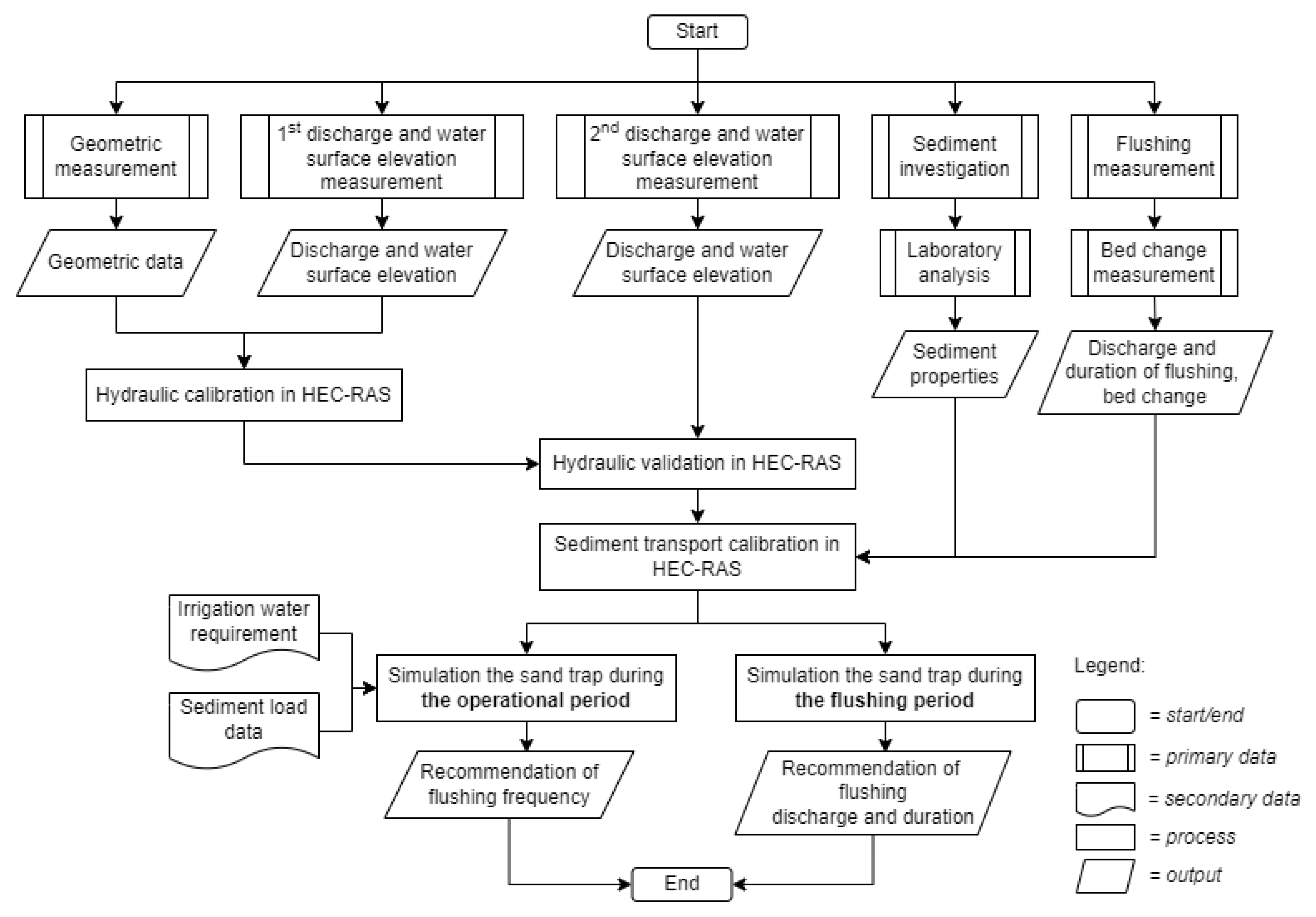
2.2. General Description of the Methodology

This study aimed to propose a management strategy of the Pengasih Weir sand trap based on mathematical modeling. We aimed to model the sand trap hydraulic behaviour during both the operational and flushing periods. During the operational phase, water flows from the irrigation intake through the sand trap body towards the primary irrigation canal. During the flushing phase, the flow travels from the irrigation intake via the sand trap body and exits through the natural channel downstream of the flushing gate. The performance level of sand traps is highly reliant on the frequency of sediment flushing [26]. According to the research flowchart, as illustrated in Figure 3, five sets of field measurements were conducted for this study.

The one-dimensional mathematical model, HEC-RAS (Hydrologic Engineering Center-River Analysis System) version 4.1, was used to simulate the sand trap during the flushing period and for ensuring sediment and hydraulic calibration and validation. HEC-RAS version 6.2 was utilized to simulate the sand trap throughout the operational period. By comparing the simulated and observed water surface elevation, the hydraulic calibration and validation were used to establish the appropriate hydraulic parameter, which was Manning’s roughness coefficient in this case. The calibration of the sediment was used to build a modeling approach for sediment transport during the flushing and operational periods of the sand trap. To estimate the appropriate operation of the sand trap, simulations were conducted during both the operational and flushing periods. During the operational phase, the irrigation water requirements and sediment load data were utilized as additional secondary data. This study recommends the frequency, discharge, and duration of flushing for the Pengasih Weir sand trap.

2.3. Data Collection

There are two types of data collection in this study, namely secondary and primary. Included in the secondary data needed are the irrigation water requirements and sediment load data. The analysis of the data was obtained from the researcher’s previous study. The irrigation water requirement is determined biweekly based on the growing phase of the paddy crop. Aside from that, the sediment load data were calculated using the Meyer-Peter and Müller equation, referencing a prior study [15]. The primary data collection consisted of geometric measurements, discharge measurements, water surface elevation measurements, sediment investigations, and flushing measures in the Pengasih Weir sand trap. The following description applies to each form of data collection.

2.3.1. Geometric Measurement

Along the channel, cross-sections were obtained from the irrigation intake to the commencement of the primary channel. Terrestrial measurements were conducted with the aid of a total station and its auxiliary components. The arrangement for the cross-section measurement process is depicted in Figure 4. Between CS_intake and CS₁₃, fourteen cross-sections were measured.

2.3.2. Discharge Measurement

The velocity was determined using a cup-type current meter. The cup is rotated in reaction to the flow velocity, and the amount of rotation is converted to the flow velocity. As velocity varies with the depth and width of the flow, the measurement was taken at a variety of depths (H) and was divided into three width segments. As seen in Figure 5, the discharge was estimated using the velocity-area approach as indicated in Equations (1) and (2). As depicted in Figure 5, there were three depth variants, namely 0.2H, 0.6H, and 0.8H, as well as three width segments. Figure 6 displays the configuration of the velocity measurement system. As can be seen, the measurement location comprised nine points. There were three cross-sections for measuring the discharge to represent the flow upstream, midstream, and downstream.

Total discharge was calculated using the velocity-area method:

$${\overline{V}}_I,{\overline{V}}_{II},{\overline{V}}_{III}=\frac{V_{0.2H}+V_{0.6H}+V_{0.8H}}{3}$$

(1)

$$Q_{tot}={\overline{V}}_I{A}_I+{\overline{V}}_{II}{A}_{II}+{\overline{V}}_{III}{A}_{III}$$

(2)

where Q_tot = total discharge, A_I, A_II, A_III = cross-sectional area of segment I, II, and III. ${\overline{V}}_I, {\overline{V}}_{II},{\overline{V}}_{III}$ = average flow velocity of segment I, II, and III; V_0.2H, V_0.6H, V_0.8H = flow velocity at a depth of 0.2H, 0.6H, and 0.8H from the water surface, B, b = channel top and bottom width, and h = flow depth.

2.3.3. Water Surface Elevation Measurement

In the HEC-RAS model, the hydraulic calibration and validation were accomplished utilizing the water surface elevation. Using an automatic level and its associated equipment, the measurement was performed. Figure 7 depicts the layout of the measurement. Evidently, there were eight cross-sections to be measured, beginning with CS₀ and finishing with CS₇. There were ten meters between the two cross-sections.

2.3.4. Sediment Investigation

The sediment properties were used for sediment modeling, and they included information about the current bed sediment in the Pengasih Weir sand trap. The sediment was sampled using a sediment grab sampler. The bed sediment sample layout is similar to that of the velocity measurement (as depicted in Figure 6); therefore, there were nine sampling points. In a soil laboratory, a given sample’s specific gravity and particle size distribution was determined using the sieve and hydrometer techniques.

2.3.5. Flushing Measurement

Some of the measured components are the flushing mechanism’s discharge and duration as well as the channel bed change. Observing the state of the channel’s bed before and after flushing, as measured by a total station, allows for the observation of changes in the channel’s bed. In the same cross-section, we conducted measurements for both situations. The bed change was employed as an input in the HEC-RAS sediment modeling.

2.4. Mathematical Modelling in Irrigation Network

The hydraulic simulation model can be a valuable tool for comprehending the hydraulic behavior of irrigation systems; it also enhances the irrigation system performance by investigating the flow characteristics in a massive and diverse irrigation network under various design and management scenarios [30]. A mathematical model can be used to analyze a vast irrigation network’s hydraulic properties and behavior, directly analyzing and enhancing the system performance [36]. Currently, technical advances allow academics to perform mathematical modeling for various goals. Numerous mathematical models are available for hydraulic modeling jobs, including the HEC-RAS, MIKE 11, CCHE1D, FLUVIAL-12, and BRI-STARS models [37,38]. These models can estimate the appearance of a river or stream after a flood, sediment transport, and clogging of reservoirs and stream channels.

This study replicates the flow and sedimentation models in a sand trap using a one-dimensional flow mathematical model and HEC-RAS version 4.1 and 6.2 [39]. The HEC-RAS model allows for the simulation of the one-dimensional water surface profile in stable rivers, unsteady river flows, as well as allowing for the simulation of delivered sediment load and river water quality [40]. The HEC-RAS one-dimensional model is extensively used to simulate sediment transport [40,41,42]. It is appropriate for evaluating the canal hydraulic steady state conditions [36]. Therefore, it can be used as a decision support system by ensuring the irrigation systems’ optimal operation and maintenance [36]. The concept of the one-dimensional energy equation was used to compute from one cross-section to another (see Equation (3)) [43,44,45].

$$Z_2+Y_2+\frac{{\alpha }_2{V_2}^2}{2g}=Z_1+Y_1+\frac{{\alpha }_1{V_1}^2}{2g}+h_e$$

(3)

where Z₁, Z₂ = elevations of the main channel bed (m); Y₁, Y₂ = depths of water at cross-sections (m); V₁, V₂ = average velocities (m/s); ${\alpha }_1,{\alpha }_2$ = velocity weighting coefficients; g = gravitational acceleration (m/s²); and h_e = energy head loss (m) due to friction and estimated by Manning’s coefficient (Equation (4)) [36,43].

$$h_e=L\overline{S_f}+C\left|\frac{{\alpha }_2{V_2}^2}{2g}-\frac{{\alpha }_1{V_1}^2}{2g}\right|$$

(4)

where L = discharge weighted reach length (m); $\overline{S_f}$ = representative friction slope between the two sections; and C = contraction/expansion loss coefficient [46,47,48].

2.5. Performance Indicators

In order to analyze the various possibilities used in this study and select the optimal option, performance indicators are required. A comparison of simulated and real-world data was involved in each scenario. We must evaluate a scenario’s accurateness in the context of the available data. To assess a recommender system’s accuracy, the root mean square error (RMSE) and mean absolute error (MAE) are typically used [49]. The model is better or the forecasts are more accurate when the RMSE and MAE are lower [50]. Equations (5) and (6) provide illustrations of these formulas [49].

$$\mathrm{RMSE}=\sqrt{\frac{{{\displaystyle \sum }}_{n=1}^N{\left({\widehat{r}}_n-r_n\right)}^2}{N}}$$

(5)

$$\mathrm{MAE}=\frac{{{\displaystyle \sum }}_{n=1}^N\left|{\widehat{r}}_n-r_n\right|}{N}$$

(6)

where ${\widehat{r}}_n$ is the prediction rating, $r_n$ is the actual rating in the testing dataset, and N is the number of rating prediction pairs between the testing data and prediction results.

Additionally, this study assessed the system utilizing the Nash–Sutcliffe efficiency index (NSE) and the coefficient of determination (R²). The correlation coefficient, abbreviated as R, measures how strongly two variables that are either of linear or straight-line relation to one another. As their linearity assumption is rarely verified, correlation coefficients are commonly employed incorrectly [50]. The coefficient of determination (R²) normally ranges from 0 to 1, with a value of 0 signifying a lack of a linear relationship and a value of 1 indicating a perfectly linear relationship [50]. In Equations (7) and (8), the coefficient of determination is described.

$$coefficient of determination={\left(coefficient of correlation\right)}^2$$

(7)

$$coefficient of correlation, R=\frac{n\left({\displaystyle \sum }xy\right)-\left({\displaystyle \sum }x\right)\left({\displaystyle \sum }y\right)}{\sqrt{\left[n{\displaystyle \sum }{x}^2-{\left({\displaystyle \sum }x\right)}^2\right]\left[n{\displaystyle \sum }{y}^2-{\left({\displaystyle \sum }y\right)}^2\right]}}$$

(8)

where R is coefficient of correlation, x are values in the first set of data, y are the values in the second set of data, and n is the total number of values.

Nash and Sutcliffe (1971) offered the efficiency index as a substitute goodness-of-fit statistic in response to the efficiency coefficient’s limitations. The NSE statistic is a frequently employed and perhaps reliable indicator of how well hydrologic models fit [51]. A linear model’s efficiency index will fall between 0 and 1 if its forecasts are unbiased. In the case of biased models, the efficiency index may be algebraically negative. Even if the model is unbiased, nonlinear models, which most hydrologic models are, can have negative efficiencies. Under the premise of a linear model, the NSE is equal to R² [51]. Equation (9) shows how to calculate the NSE.

$$\mathrm{NSE}=1-\frac{{{\displaystyle \sum }}_1^n{\left({\widehat{Y}}_i-Y_i\right)}^2}{{{\displaystyle \sum }}_i^n{\left(Y_i-\overline{Y}\right)}^2}$$

(9)

where ${\widehat{Y}}_i$ is the predicted value of the criterion (dependent) variable Y, $Y_i$ is the measured value of the criterion (dependent) variable Y, $\overline{Y}$ is the mean of the measured values of Y, and n is the sample size.

3. Results and Discussion

3.1. Data Collection Results

There were two stages to the primary data collection process. Sediment sampling (to be tested in a soil laboratory), measurements of the discharge and water surface elevation under normal flow circumstances (operational phase), measurements of the channel cross-section, dimensional measurements of inline structures, and measurements of discharge and flushing duration (flushing phase) comprised the first stage of data collection. Measurements of the cross-section were made both before and after flushing. When the sand trap is flushed, it indicates that the sediment has been removed from it and that it was previously full of sediment. These two circumstances can be used to calculate the amount of sediment that accumulates in the sand trap over the operational period. Discharge and water level measurements comprised the second stage of data collection. In order to set up the geometry and perform the hydraulic calibration, the first measurement datasets of discharge, water surface elevation, and cross-section were used. The second measurement datasets of discharge and water surface elevation were used for the hydraulic validation. Additionally, the sediment calibration used the dataset of the sediment sampling, bed change, and discharge and flushing duration.

Table 1. Summary of the collected primary data.

No.	Type of Data	Results	Note
1.	Average discharge
	■ From the first stage, under operational phase	2.03 m3/s	Average flow depth: 1.56 m; average velocity: 0.19 m/s
	■ From the second stage, under operational phase	0.53 m3/s	Average flow depth: 1.20 m; average velocity: 0.08 m/s
2.	Water surface elevation
	■ From the first stage, under operational phase	8 values (in meters)	From station 0–70: 96.416, 96.409, 96.401, 96.436, 96.435, 96.384, 96.383, 96.382
	■ From the second stage, under operational phase	8 values (in meters)	From station 0–70: 95.741, 95.730, 95.730, 95.724, 95.718, 95.702, 95.702, 95.702
3.	Sediment
	■ Average specific gravity	2.66	Based on pycnometer test
	■ Grain size distribution		Based on sieve and hydrometer test
	○ Upstream (Station 10)	9 values (in % finer)	VFG: 99.58, VCS: 98.48, CS: 94.49, MS: 76.97, FS: 48.86, VFS: 9.66, CM: 5.59, FM: 2.20, Clay: 0
	○ Midstream (Station 30)	9 values (in % finer)	VFG: 99.08, VCS: 98.81, CS: 98.43, MS: 79.30, FS: 60.11, VFS: 22.16, CM: 13.29, FM: 10.54, Clay: 0
	○ Downstream (Station 50)	9 values (in % finer)	VFG: 95.87, VCS: 91.58, CS: 87.30, MS: 74.41, FS: 60.54, VFS: 18.03, CM: 11.29, FM: 6.92, Clay: 0
4.	Discharge and duration of flushing
	■ Discharge	2.08 m3/s	Average flow depth: 0.30 m; average velocity: 1.59 m/s
	■ Duration	90 min
6.	Volume of sediment deposited during the operational period at the time of measurement (within 80 days)	36.51 m3	based on cross-section measurement
7.	Capacity of sand trap	84.40 m3	based on cross-section measurement
8.	Length of sand trap	100 m

Where VFG is very fine gravel, VCS is very coarse sand, CS is coarse sand, MS is medium sand, FS is fine sand, VFS is very fine sand, CM is coarse silt, and FM is fine silt.

displays the results of the primary data collection in summary.

3.2. Preparation of Model

Hydraulic modeling was performed to provide important information about the performance of the Pengasih Weir sand trap during the operational and flushing periods. A hydraulic simulation model is a mathematical representation of the physical hydraulic processes that occur in the field. Such processes can be described by the conservation of mass, conservation of momentum, and conservation of energy equations, posed in either one, two, or three dimensions. In one-dimensional hydraulic modeling, the flow is assumed to move in the longitudinal direction only, that is, downstream. This study employed the one-dimensional HEC-RAS model version 4.1 and 6.2 to simulate the sand trap during the operational and flushing periods. This is attributed to the sand trap being an artificial channel with uniform lining and a narrow width; therefore, the predominant flow direction is in the longitudinal direction.

The procedure for performing flow simulations using the HEC-RAS model consists of five components [39]: model preparation, geometry modeling, flow modeling, hydraulic computation, and presentation and interpretation of simulation results. This study used geometry and flow datasets to estimate the operational and flushing phases. Figure 8 displays the geometry in the operational and flushing periods. The green arrow denotes the flow direction in the operational period. The geometry in this period was used for hydraulic calibration and validation. The water flows from the irrigation intake through the body of the sand trap and into the primary irrigation canal. The orange arrow depicts the flow direction during the flushing period. The geometry in this period was used to calibrate the sediment. The flow travels from the irrigation intake through the sand trap body and escapes through the natural channel downstream of the flushing gate. The user must always replicate the river reach in the upstream–downstream direction when using HEC-RAS. Consequently, the most downstream segment of the reach is designated as river station 0.

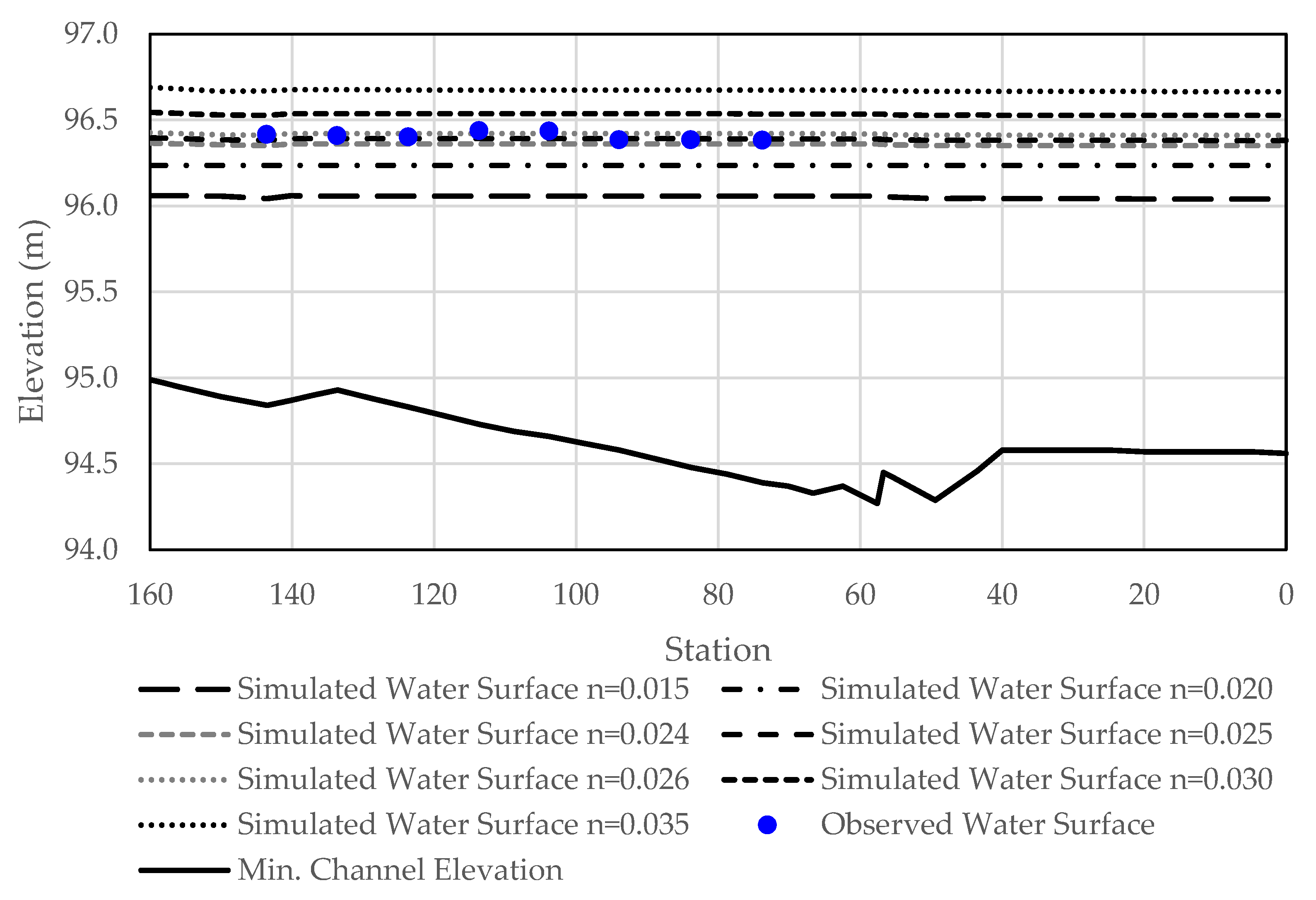
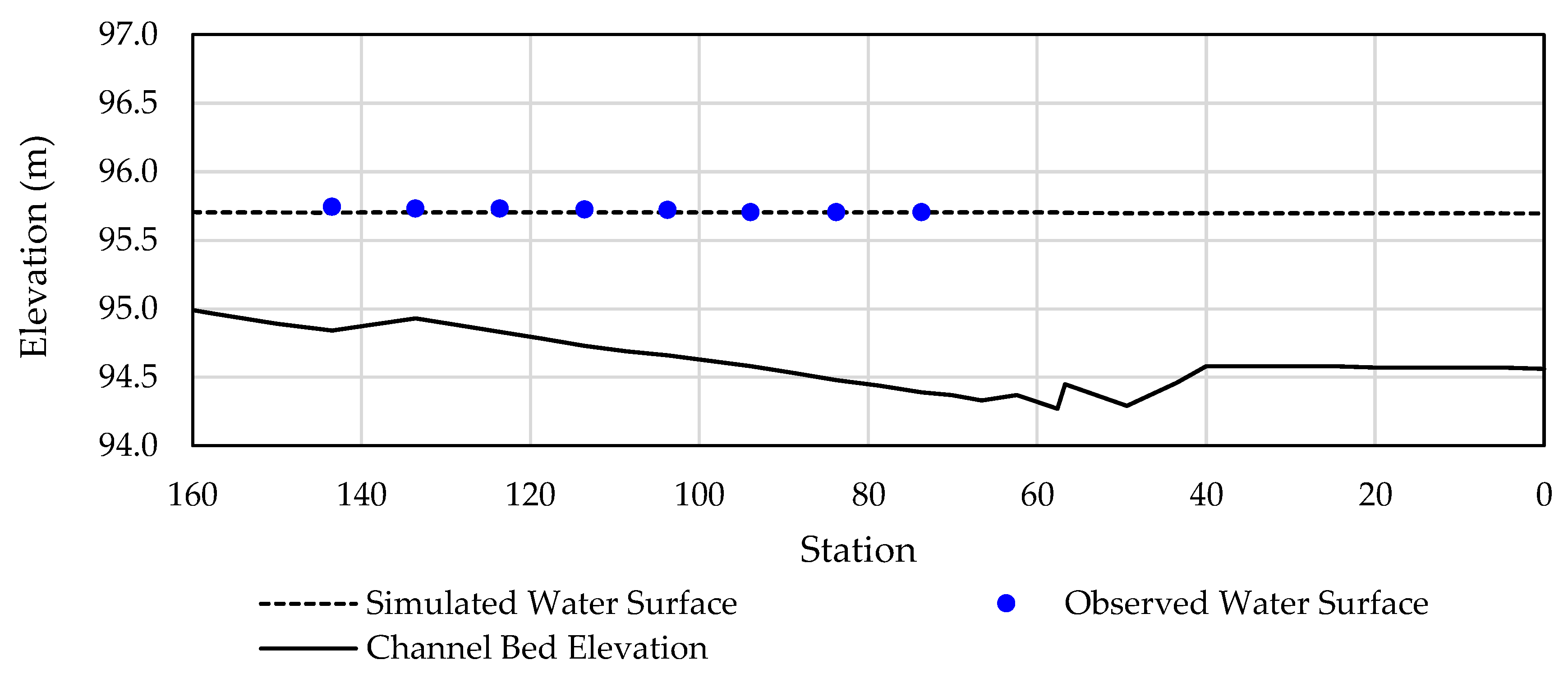
3.3. Hydraulic Calibration and Validation

In both hydraulic calibration and validation, flow and water surface elevation data from the two independent measurements obtained at different times were utilized. The flow was treated as a steady flow as it takes place in a channel with a uniform shape, and the discharge remains constant throughout time. As depicted in Figure 8, the operational geometry was utilized for both hydraulic calibration and validation. A normal discharge of 2.03 m³/s was utilized as an input for the steady flow data in the calibration process. The condition at the downstream boundary was normal depth. In addition, the observed water surface elevation was input into the flow model and compared with the estimated elevation. There were eight points of data for the elevation of the water’s surface, with values ranging from +96.382 m to +96.436 m.

Obtaining Manning’s bed roughness coefficient, which was used in the simulation, was the initial step of the calibration process. According to field observations, the sidewalls and bottom of the Pengasih Weir sand trap channel are composed of stone laid in mortar; Manning’s coefficient table, which is accessible via the HEC-RAS model, does not fully account for this type of configuration. As a strategic approach, we opted for a concrete bottom float with random stone on the mortar sides, with minimum, average, and maximum values of 0.017, 0.020, and 0.024, respectively. As a result, the Manning coefficient for the initial simulation was assigned at 0.015. Figure 9 depicts the hydraulic calibration results. Various Manning coefficients were used to compare the observed and simulated water surfaces. The upstream and downstream sections of the sand trap are on the right and left sides of the diagram, respectively. The blue dashed lines illustrate the Manning coefficient-calculated water levels. We also plot the channel bed elevation in a straight black line to provide a sense of the channel depth during the simulation.

As illustrated in Figure 9, the water surface elevation that was predicted using the input Manning’s coefficient of 0.015 is underestimated, with the overall trend being below the reported water level. The Manning’s coefficient was changed in the following simulation to 0.020; however, the simulated water level elevation was still underestimated. The simulation was then performed with a Manning’s coefficient of 0.025, and it can be seen that the observed water surface conforms to the simulation’s water level elevation. The simulation was then conducted with a Manning’s coefficient of 0.030 to determine whether the value of 0.025 is appropriate. It is absolutely noticeable that the findings are overstated. We determined that the value of 0.025 for Manning’s coefficient appeared closest to the observed water surface. Furthermore, we added two Manning values close to 0.025, namely 0.024 and 0.026, to confirm the calibration results. We analyzed the accuracy of the calibration results obtained using performance indicators such as the coefficient of determination (R²), Nash–Sutcliffe efficiency index (NSE), root mean square error (RMSE), and mean absolute error (MAE), as shown in

Table 2. Performance indicators of the calibrated Manning’s coefficient.

No.	Performance Indicator	Value
		n = 0.015	n = 0.020	n = 0.024	n = 0.025	n = 0.026	n = 0.030	n = 0.035
1	Coefficient of Determination (R2)	0.9379	0.9457	0.9369	0.9522	0.9474	0.9477	0.8051
2	Nash–Sutcliffe Efficiency Index (NSE)	−282.7061	−68.1269	−4.8787	−0.6402	−0.5346	−38.6501	−166.5715
3	Root Mean Square Error (RMSE)	0.3505	0.1730	0.0504	0.0266	0.0258	0.1310	0.2693
4	Mean Absolute Error (MAE)	0.3497	0.1716	0.0456	0.0216	0.0224	0.1293	0.2685

[49,50,51]. As can be seen, the outcomes from the Manning’s value of 0.025 perform well across all indicators, even if compared with those of 0.024 and 0.026. If we look at the comparison between the performance indicators of Manning 0.025 and 0.026, only the RMSE value of Manning 0.026 was slightly better than that of Manning 0.025. For the R² and NSE values, the closer they are to one, the better, while for RMSE and MAE, the smaller their error, the more accurate. When the observed data are a better predictor than the model, particularly for NSE, an efficiency below zero occurs. Negative efficiencies are possible with nonlinear models, of which most are hydrologic [51]. As a result, a negative NSE value is permitted. Therefore, it can be concluded that 0.025 is best suited for the Manning’s roughness coefficient of the channel condition of the Pengasih Weir sand trap. This condition is referred to as the calibrated Manning’s coefficient.

After calibrating the Manning’s coefficient to the required accuracy of 0.025, the second measurement dataset was utilized to validate the coefficient. The input for the steady flow data was a normal discharge at a rate of 0.53 m³/s. The condition at the downstream boundary was normal depth. In addition, the observed water surface was incorporated into the process of flow modeling, which would be compared with the simulated water surface. There were eight points of data for the elevation of the water’s surface, with values ranging from +95.702 m to +95.741 m. Figure 10 represents the results of the hydraulic validation. It compares the observed and simulated water surfaces at n = 0.025. The validated Manning’s coefficient generates a water surface that is compatible with the observed data, as illustrated. As with the calibrated Manning’s coefficient, the verified one was evaluated using performance metrics such as R², NSE, RMSE, and MAE (see

Table 3. Performance indicators of the validated Manning’s coefficient.

No.	Performance Indicator	Value, n = 0.025
1	Coefficient of Determination (R2)	0.8479
2	Nash–Sutcliffe Efficiency Index (NSE)	−0.9833
3	Root Mean Square Error (RMSE)	0.0221
4	Mean Absolute Error (MAE)	0.0168

). The outcomes perform admirably across the board. Specifically, for NSE, a sub-zero efficiency occurs when the observed data outperform the model’s forecast. Consequently, 0.025 was declared as the validated Manning’s coefficient, and it can be utilized in the simulation of sediment models. For defining water flow through the ground, Manning’s roughness coefficient is one of the most significant quantities. Surface irrigation field conditions widely vary, and it is not clear how to accurately measure this roughness factor. This procedure can be used as a reference in dealing with the problem.

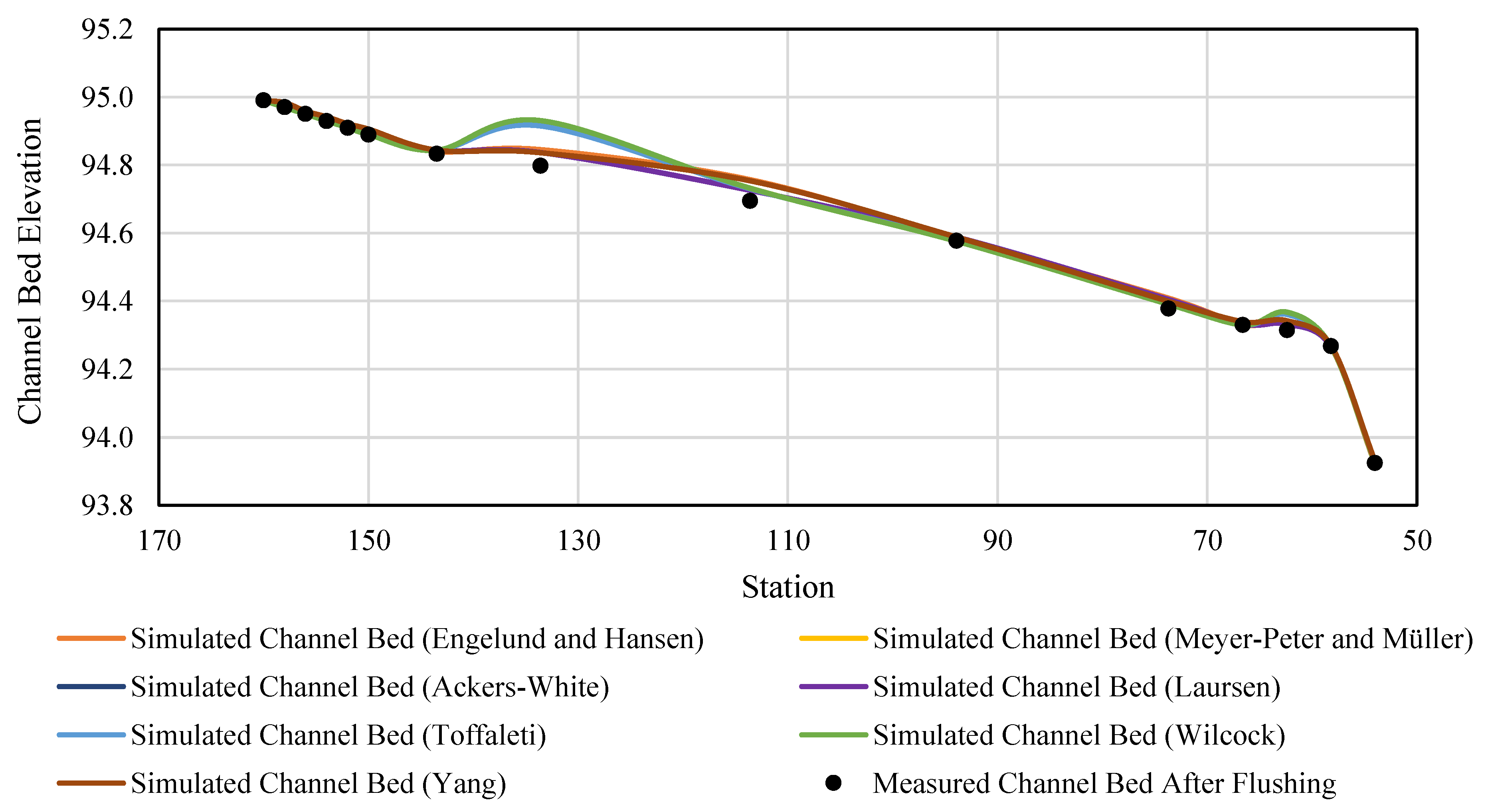
3.4. Sediment Calibration

A correct estimation of erosion and sedimentation at a stream cross-section depends on the sediment transport equation selection and Manning roughness coefficient [37]. Using the sediment transport concept, one can model the flushing in the sand trap of an irrigation network. The intricacy of sediment transport modeling is well-known. The data utilized to predict bed changes are uncertain, and the underlying theory is empirical and extremely sensitive to a wide range of physical variables [47]. With sufficient data, however, it is possible to calibrate regional sedimentation models to construct decision plans and assess sedimentation issues. Before the HEC-RAS model can compute the sediment transport, the sand trap hydraulics parameter must be established. The HEC-RAS model employs a hydrodynamic simplification, which numerous sediment transport models also utilize. The assumption of a quasi-unsteady flow is similar to a continuous hydrograph with several different steady flow patterns.

The maximum amount of sediment that can leave the control volume depends on how much sediment the water can transport. The term that refers to this is sediment transport capacity. Sediment transport potential, which measures how much material of a particular grain class a given hydrodynamic condition can carry, is a factor that must be determined in order to compute the sediment transport capacity. Seven sediment transport potential function equations, including the Ackers and White (1973), Engelund and Hansen (1967), Laursen–Copeland (1968, 1989), Meyer-Peter and Müller (1948), Toffaleti (1968), and Yang (1973, 1984) equations, are accessible in HEC-RAS version 4.1 [47].

The sediment transport potential is determined according to the grain size fraction, enabling the simulation of hydraulic sorting and armoring. The bed sorting method (also known as the mixing or armoring method) records the bed gradation that HEC-RAS uses to compute the grain class specific transport capacity and simulate the supply-side armoring procedures. The most common result of bed sorting is armoring, which occurs when a coarse cover layer forms on top of a more representative subsurface layer of the river bed material. The active layer and Exner 5 are the two possible sorting methods in HEC-RAS version 4.1. In addition, the fall velocity technique is believed to be consistent with the evolution of the sediment transport function. The four selectable modes are the Rubey, Toffaleti, Van Rijn, and Report 12 modes. The researcher must find the optimal sediment transport model methodology for a given case, location, and environmental condition, including sorting and velocity methodologies. In order to improve the prediction of the sediment transport capacity, it is also essential to establish the correct transport potential function. To overcome this issue of identifying the sediment transport modeling strategy, calibration is essential. The calibration parameter can be found by looking at how the bed changes when sediment is flushed.

In this study, we measured the changes to the bed following sand trap flushing. A comparison was made between the simulated and observed bed changes for calibration. The sediment transport simulation consists of eight scenarios, comprising the two sorting and four fall velocity algorithms indicated in

Table 4. Scenarios for the sediment calibration.

Scenario	Sediment Transport Parameter
	Sorting Method	Fall Velocity Method
1	Active Layer	Rubey
2	Active Layer	Toffaleti
3	Active Layer	Van Rijn
4	Active Layer	Report 12
5	Exner 5	Rubey
6	Exner 5	Toffaleti
7	Exner 5	Van Rijn
8	Exner 5	Report 12

. Each scenario is represented by a graph of seven potential transport functions. A plan in HEC-RAS represented the scenario; hence, eight sediment transport plans were calculated. The HEC-RAS output that was considered was a sediment spatial plot; it displayed the bed level after a specified duration of flushing. The actual flushing of the Pengasih Weir sand trap took 90 min and generated a flow at a rate of 2.08 m³/s. Consequently, each simulation lasted 90 min.

The elevation of the simulated channel bed after 90 min of flushing was compared with the measured elevation using multiple transport functions available in HEC-RAS version 4.1. We ran simulations of each transport function using the eight specified scenarios. For each scenario, the combination of all transport functions was graphed. Then, it was determined which of the simulated bed elevations produced by all of the combinations was the one that came closest to matching the observed bed elevation following flushing. We discovered that scenario five, specifically from the transport potential function of the Laursen method, provided the most accurate bed elevation comparison. Figure 11 depicts the comparison of the bed elevation from scenario five. The left side of the graph represents the upstream region, while the right side indicates the downstream region. In Figure 11, the dots represent the observed channel bed after flushing, whereas the purple line represents the Laursen-simulated channel bed. The closest line to the dots is the purple one. We then tested the simulation using the performance metrics listed in

Table 5. Performance indicators of the sediment calibration.

No.	Performance Indicator	Value
1	Coefficient of Determination (R2)	0.9986
2	Nash–Sutcliffe Efficiency Index (NSE)	0.9974
3	Root Mean Square Error (RMSE)	0.0163
4	Mean Absolute Error (MAE)	0.0114

, specifically R², NSE, RMSE, and MAE. According to Table 5, all values are acceptable. Consequently, using Laursen for the potential function, Exner 5 for the sorting method, and Rubey for the fall velocity method are the optimal approaches we determined for the modeling of sediment movement in this scenario.

When the actual condition is considered, using Laursen as a transport function makes sense in this scenario. The Laursen equation was developed for gravel transport and extended down into the silt range. None of the other functions currently included in the HEC-RAS model are explicitly designed for silt-sized particles [47]. This investigation determined the bed gradation, ranging from fine gravel to fine silt. It is consistent with the Laursen equation of the transport function’s identification. In terms of sorting, Exner 5 armoring techniques have been successfully applied to various river systems. As a result, it was also appropriate for this investigation. Rubey’s calculating fall velocity is also suitable for silt, sand, and gravel grains. Furthermore, Rubey recommended particles with a specific gravity of 2.65 as optimal for the equation [47]. From the laboratory test result, the specific gravity of the sediment for this study is 2.66.

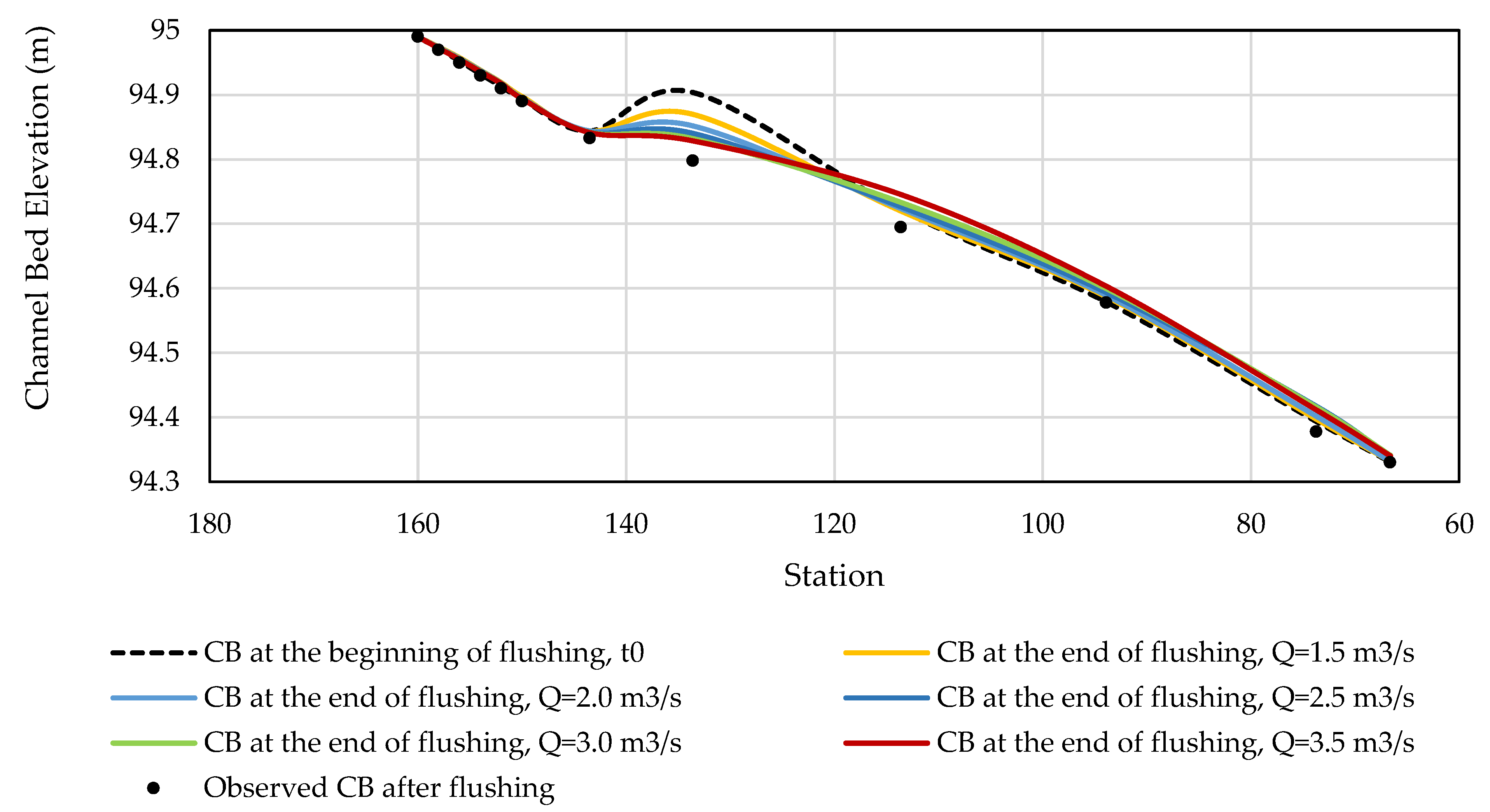
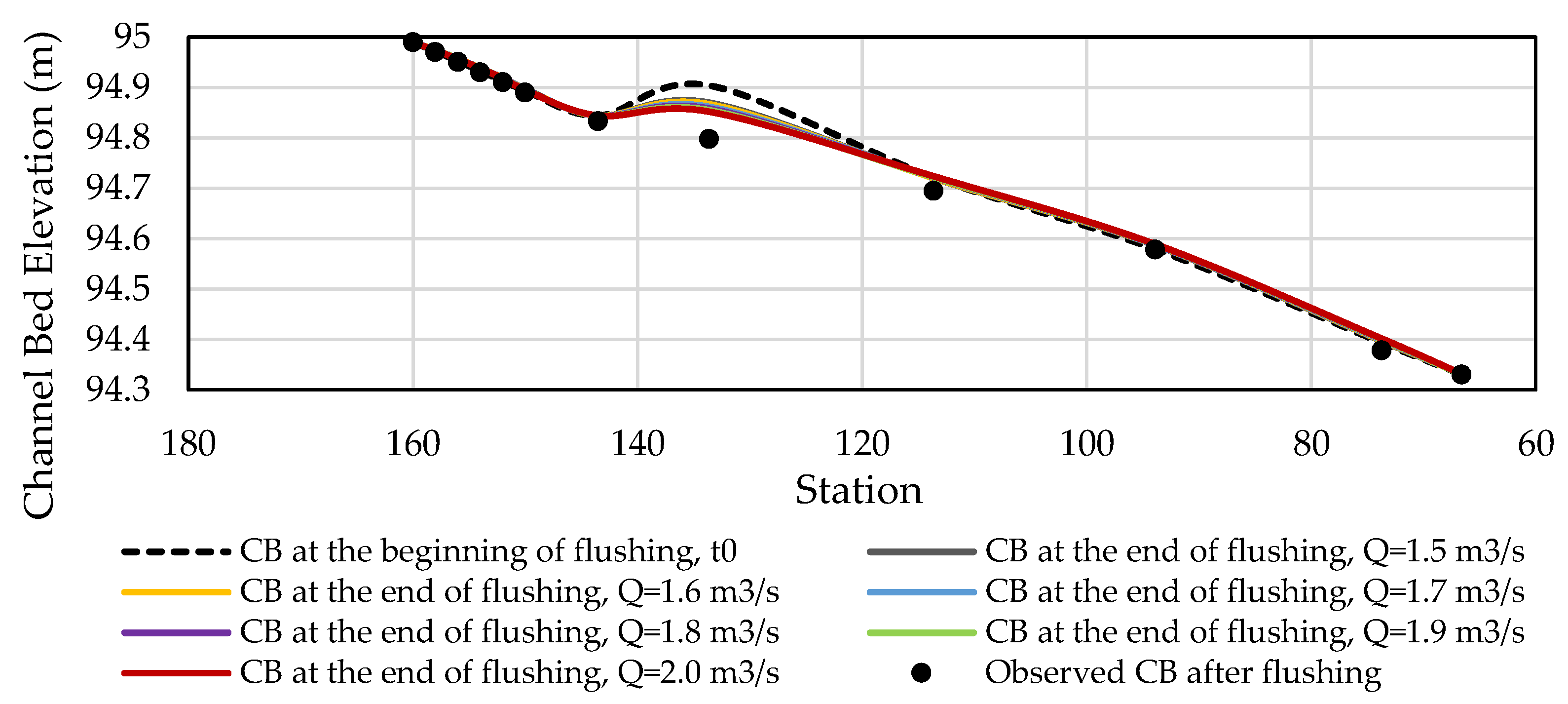
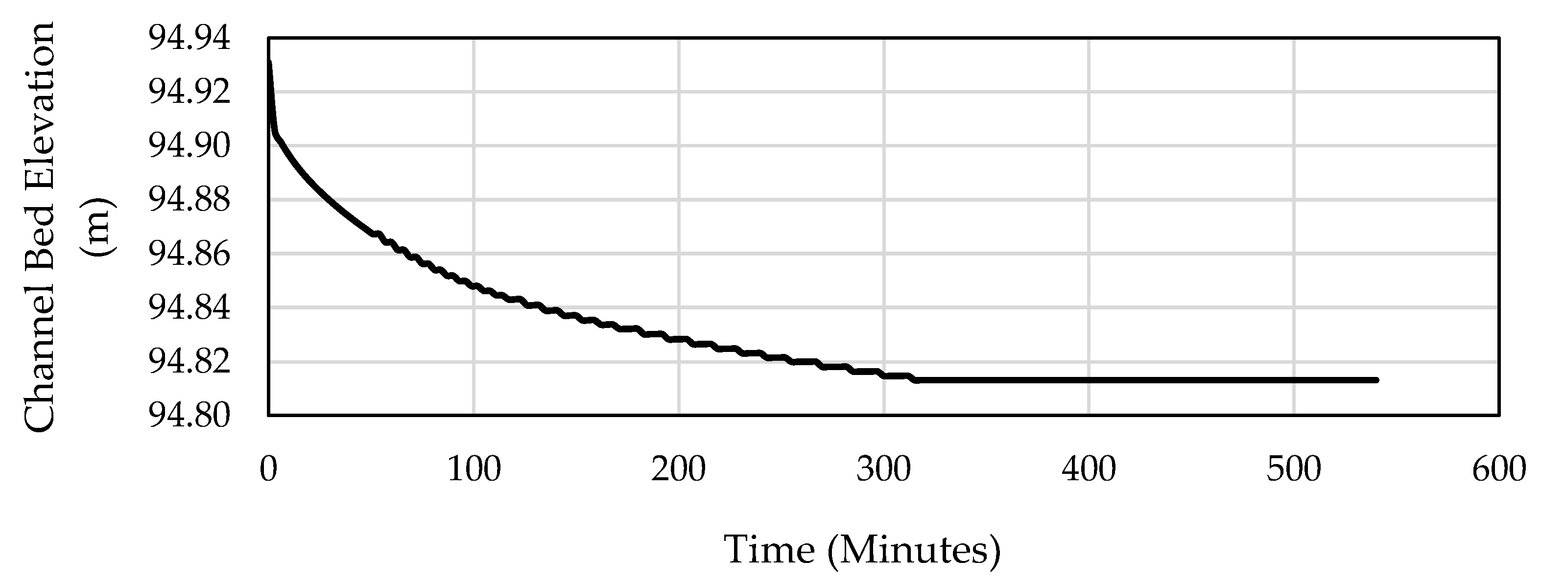
3.5. Simulation of Sand Trap Model in Flushing Period

The approach for modeling the sediment transport was determined in the previous step. The subsequent analysis is a simulation of the flushing, which analyzes the efficacy of various sand trap flushing discharges over 90 min. The flushed bed elevation from the simulation was then compared with the observed dataset. The flushing process was replicated for 90 min with five distinct discharges separated by increments of 0.5 m³/s. These discharges were 1.5, 2.0, 2.5, 3.0, and 3.5 m³/s. The actual flushing discharge, 2.08 m³/s as determined by the field measurement, serves as the reference for determining the discharge values. Figure 12 depicts the results of the simulation. The left part of Figure 12 shows the upstream region, whereas the right leg represents the downstream region. Each scenario’s line terminates at station 66.6, the final stop before the flushing gate. This is due to the evaluation’s emphasis on the sand trap’s inside while ignoring its downstream. The dotted black line represents the channel bed prior to flushing. At station 133.6, where the bed slope bends, a substantial amount of sediment was deposited, resulting in a sediment thickness of 10.57 cm; this value is determined by the difference in bed elevation before and after flushing at that particular station.

As shown in Figure 12, all discharges led to a comparable decrease in the amount of material dumped near station 133.6 and a rise in sediment deposition in the downstream of station 133.6. Each simulated channel bed (after flushing) was compared with the observed channel bed using R², NSE, RMSE, and MAE as performance indicators. The performance indicators for the sediment simulation results are summarized in

Table 6. Performance indicators of the sediment simulation results.

Performance Indicators	Values from the Discharge of
	1.5 m3/s	2.0 m3/s	2.5 m3/s	3.0 m3/s	3.5 m3/s
R2	0.9972	0.9981	0.9975	0.9973	0.9968
NSE	0.9956	0.9968	0.9954	0.9950	0.9943
RMSE	0.0212	0.0181	0.0217	0.0226	0.0241
MAE	0.0127	0.0117	0.0149	0.0156	0.0161

. As can be seen, the performance of the 2.0 m³/s discharge is superior to that of the 1.5 m³/s discharge. The values are all acceptable.

The optimization procedure was then carried out based on the simulation results. The flushing simulation lasted for 90 min with six distinct discharges ranging from 1.5 to 2.0 m³/s. The interval was reduced from 0.5 to 0.1 m³/s, thus the discharges became 1.5, 1.6, 1.7, 1.8, 1.9, and 2.0 m³/s. Figure 13 depicts the results. As can be seen, the graphs provide almost identical results. Compared with the bed changes that were made after 90 min of flushing, the 0.1 m³/s difference in discharge is insignificant. Based on Figure 14, the red line shows that the channel bed caused by a 2.0 m³/s discharge was the most similar to the actual data, with the performance indicators shown in the second column of Table 6.

According to the observations, a discharge rate of 2.0 m³/s is acceptable for the flushing of the Pengasih Weir sand trap. According to the measurements taken in the field, the average flushing outflow was 2.083 m³/s. The present methods for discharge and flushing could be argued to be already suitable and practical. Additionally, considering the flushing duration, the more efficient the flushing operation, the shorter its duration. Nevertheless, the sediment was not completely flushed during the actual time (90 min), especially at station 133.6. Because there is a bend in the bed slope, this station represents the predominant cross-section, where the greatest amount of sediment was deposited in the Pengasih sand trap. We could utilize the station to determine the duration of flushing until the entire sediment volume is cleared.

The time series for the flushing of the sediment, specifically that which accumulated in station 133.6, is depicted in Figure 14. The straight line of the curve suggests that all sediment has been flushed. Therefore, the recommended flushing timeframe is 315 min, or 5.25 h. To regulate the flushing process, we must consider the amount of available water in the source river. If the minimum discharge of the river exceeds 2.0 m³/s, the flushing operation can be carried out. The institution responsible for irrigation in the Kulon Progo Regency, which contains the Pengasih Weir, has installed a number of automatic water level recorders (AWLRs) at present. They were built in various locations throughout the Pengasih irrigation scheme, including one on the side of the weir. These help the operator flush the sand trap.

In addition to the water availability in the source river, we must also consider the irrigation water requirements of the rice crop. Priority should be placed on water usage if they are in the cultivation and growth stages. Sedimentation problems begin in the upstream portion of the irrigation system and continue throughout the network to the downstream part. If upstream efforts to prevent sedimentation are still optimal, it is vital to investigate the reasons and solutions of sedimentation issues that arise along the network. This is essential for sustaining the long-term viability of the irrigation system, which is a national strategic priority that would promote more remarkable agricultural production. Good agricultural products can lead to food self-sufficiency, which contributes to achieving Sustainable Development Goal 2: end hunger, achieve food security, improve nutrition, and promote sustainable agriculture.

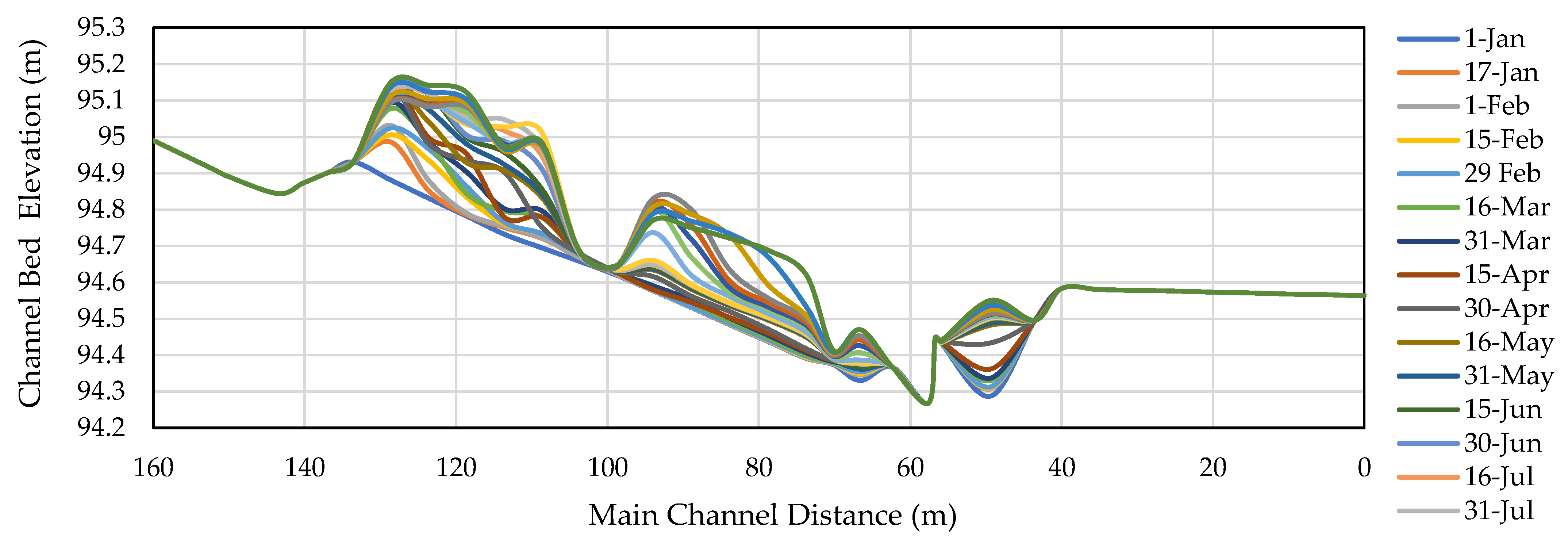
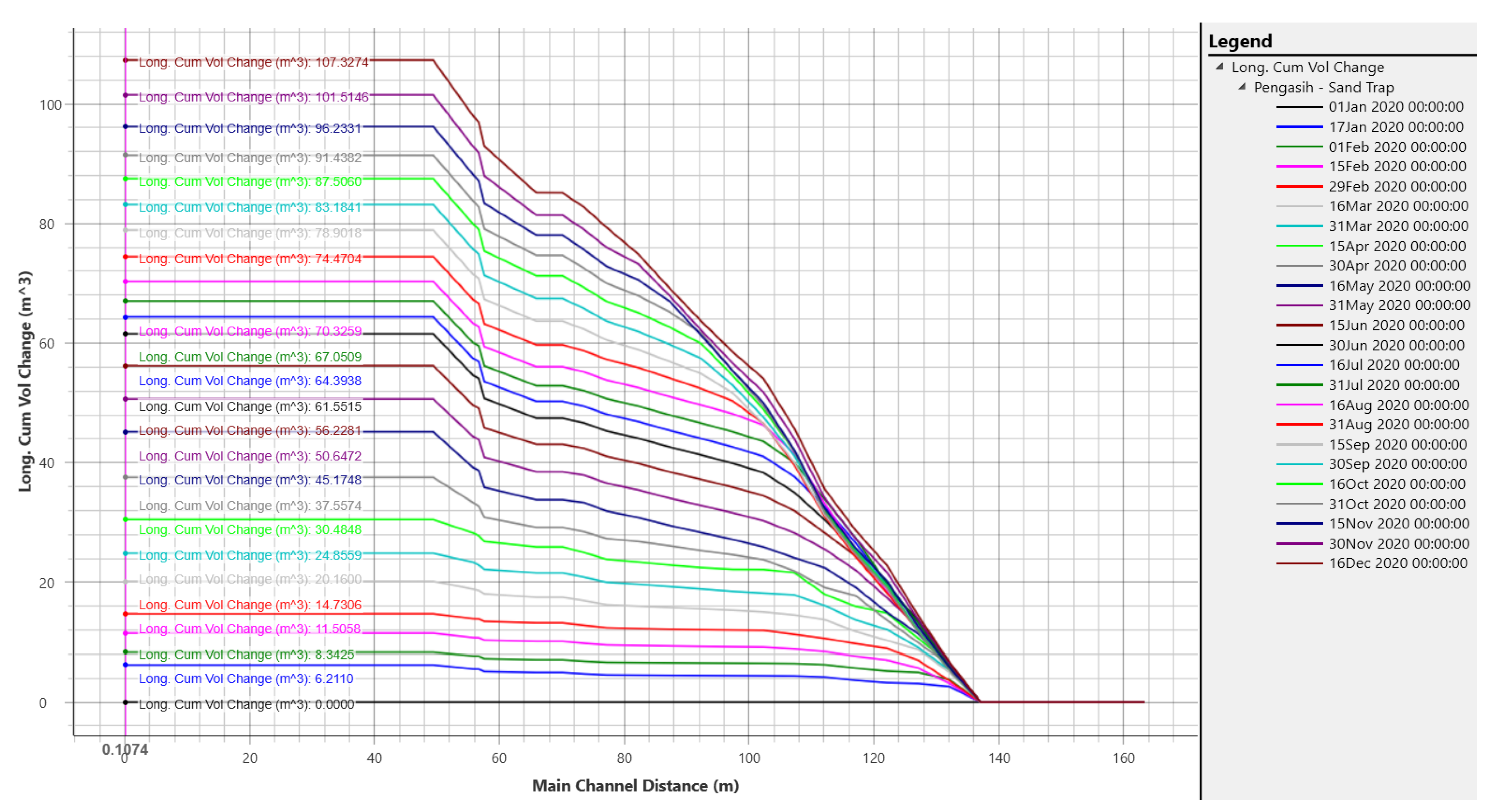
3.6. Simulation of Sand Trap Model in Operational Period

During the operational period, the flushing gate downstream of the sand trap is closed, allowing the flow to enter the primary irrigation channel. In this period, the flow of irrigation water is distributed through the primary, secondary, and tertiary irrigation networks to meet the water needs of the crops in the paddy fields. At the same time, sediment that enters through the irrigation intake will slowly settle in the sand trap. Sand traps are designed with a specific capacity; if this capacity is met, the sediment will enter the primary irrigation network. Obviously, this is not expected as it will reduce the channel capacity and overall irrigation efficiency. As previously stated, the Indonesian government has been executing an irrigation modernization program to address various problems, and one of the indications of modernization is a better irrigation efficiency. Therefore, it is necessary to assess the behavior of the sand trap in the operational period with the indicator of flushing frequency.

The officer determines the frequency of flushing in the field solely based on the adequacy of the river’s discharge and whether the rice plants require water at that time. Therefore, it can be stated that the frequency of flushing in the field is only determined on the basis of estimates and observations, not on the sand trap’s capacity. According to a literature review, the Pengasih Weir sand trap has a capacity of 84 m³ [15]. Pradipta et al. (2020) assessed the time required for the Pengasih Weir sand trap to attain the full condition using analytical calculations based on the Meyer-Peter and Müller and Einstein sediment transport equations [15]. Both equations can be applied to the properties of the bottom sediment under the conditions of constant flow while disregarding the wash load [15]. Using the same input properties of flow, channel hydraulics, and sediment, the Meyer-Peter and Müller and Einstein equations yielded different times to achieve the maximum capacity, namely 162 (5.4 months) and 274 (9.1 months) days, respectively [15]. According to the weir operator, the sand trap was flushed after 80 days in 2019. It can be claimed that the frequency of draining was less efficient because it was performed before the sand trap had reached full capacity.

The results of the analytical calculations from Pradipta et al. (2020) need to be validated by mathematical modeling, which in this study was carried out using HEC-RAS version 6.2. The reason for using the latest HEC-RAS version for modeling a sand trap in the operational period is that it can provide a more diverse sediment output compared with version 4.1 (the version used in modeling a sand trap in the flushing period). There are three types of sediment output in HEC-RAS version 4.1: sediment spatial plot, sediment time series plot, and sediment–XS bed change plot. The three output types are sufficient to represent the expected modeling results in the flushing period. In HEC-RAS version 6.2, there are various sediment outputs, including Froude number channel, invert change, invert elevation, longitudinal cumulative volume change, Manning’s n channel, shear stress, cumulative bed volume change, etc. In both versions of the HEC-RAS mentioned, users can also select sediment output options in groupings of output level, mass/volume, output increment, etc.

Similar to the modeling during the flushing period, we modeled the geometry, quasi-unsteady flow data, and sediment data throughout the operational period. We employed the geometry depicted in Figure 9. There are three boundary conditions for the quasi-unsteady flow data: upstream, middle, and downstream. In line with the rice crop’s growth phase, the upstream section (station 160) was fitted with a flow series containing data in the form of irrigation water requirements for two weeks for one year. The water demand for irrigation in Pengasih ranges from 0.4 to 2.22 m³/s. The middle portion (station 55.6) was specified as a time series gate opening, assuming that the gate is always fully open. The downstream part (Station 0) was set to normal depth. There are two primary inputs in the sediment data section: initial conditions and transport parameters and boundary conditions. In the initial conditions and transport parameters, we employed the parameters based on the calibration results stated in Section 3.4, where the transport function was Laursen, sorting method was Exner 5, and fall velocity method was Rubey. Regarding the initial conditions, we modeled the sand trap to the empty condition. In the section on bed gradation, measurement results taken upstream of the sand trap were utilized. In the section on boundary conditions, we provided two sets of flow-load rating curves. Based on the field measurements, we acquired two flow rates of 2.03 and 0.53 m³/s, which we also utilized for the hydraulic calibration and validation. At the same time, the two total load values were derived from the analytic calculations according to Pradipta et al. (2020).

Figure 15 represents the results of the sediment transport modeling during the operational period. The values are presented every two weeks according to the irrigation requirement discharge settings in the Pengasih irrigation scheme. From the intake (station 160) to station 133.6, the upstream portion of the sand trap was modeled with “pass-through nodes” in the sediment data setting option in HEC-RAS, indicating that no sediment is permitted to deposit in this area. This is because the area is included in the ineffective flow area due to the inflow from the irrigation intake. During the operational period, there was no sediment deposition in this location, according to field observations. Figure 16 indicates that the sediment entering the sand trap via the Pengasih irrigation intake was not uniformly deposited. Most sediment accumulates upstream towards the middle and downstream before entering the primary irrigation canal. It indicates that the greatest sediment deposition occurred in the sand trap’s upstream region. In Section 3.4’s discussion, it was reported that there was a bend in the slope of the channel bottom upstream of the sand trap, precisely at station 133.6. This requires additional thought and consideration. The bend also reduces the effectiveness of the flushing procedure as well as the operational of the sand trap in general. It is recommended that the government in charge of irrigation in the Kulon Progo Regency (where the Pengasih irrigation network is located) carry out a rehabilitation program to solve the bending issue and improve the sand trap’s performance. Irrigation network rehabilitation is the process of repairing or upgrading irrigation systems in order to return or enhance irrigation capabilities and services for the purposes of expanding planting area and/or intensifying agricultural production.

To determine how long it will take for the sand trap to achieve its maximum capacity, we plotted the cumulative volume change every two weeks, as shown in Figure 16. As can be observed, the cumulative volume deposited in the sand trap on September 30 is 83.18 m³, whereas the cumulative amount for the subsequent biweekly period (October 16) is 87.51 m³. It can be observed that the sand trap nearly achieved its full capacity of 84 m³ by the end of September. If we compare it with the results of the analytical calculations conducted by Pradipta et al. (2020), it was found that the sand trap will reach full capacity after 9 months based on Einstein’s sediment transport equation. The results of these two studies imply that the Pengasih irrigation network’s sand trap should be flushed roughly every nine months or in September of each year.

In addition to considering the sediment transport factor in the sand trap as modeled in this study, the flushing of the sand trap must also include the following factors: (i) the demand for irrigation water in paddy fields; and (ii) the availability of river water. The Pengasih irrigation scheme is incorporated into Kulon Progo’s Kalibawang irrigation interconnection system. Kulon Progo is one of four regencies in Indonesia’s Yogyakarta Special Region. In Kulon Progo, there are three groups of irrigation schemes governed by three different authorities: the Kalibawang irrigation scheme, which falls under the jurisdiction of the central government; the Sapon irrigation scheme, which falls under the jurisdiction of the provincial government; and the Small irrigation schemes, which falls under the jurisdiction of the district government. As stated in Section 2.1, the Pengasih irrigation area receives water from the Serang River (with an average annual discharge of 2.8 m³/s), with the part of the Serang River leading to Pengasih being supplemented by the Kalibawang main canal. The Kalibawang main canal is the principal irrigation water supply channel for the Kulon Progo Regency. The Kalibawang intake is the essential structure of the Kalibawang irrigation network as it collects water from the Progo River (with an average annual discharge of 7 m³/s) for distribution to the rice fields via the main channel and tertiary canal. The planting design in the Kalibawang irrigation scheme applies a group system based on the availability of irrigation water discharge and the area, namely group I and II. Group II includes the Pengasih irrigation scheme in this instance.

In group II, the first planting season, or MT-1 (paddy), begins in November 2021 and completes at the end of March 2022; the second planting season, or MT-2 (paddy), takes place from April to July 2022. The third planting season, or MT-3 (“palawija” or vegetables), begins in August and finishes at the end of October 2022, according to the Kulon Progo Regency Regulation Number 39 of 2021 regarding the annual planting system for 2021. It is to be noted that the term palawija comes from Sanskrit, which can be interpreted as a second crop in the dry season. On the basis of this cropping pattern, irrigation water requirements for one planting season can be determined. As previously stated, flushing the sand trap also takes into account the irrigation water needs and the availability of river discharge in addition to the sediment transport factor, as well as the time required to attain full capacity. Figure 17 depicts the annual water balance for the Pengasih irrigation scheme.

Regarding Figure 17, the requirement for irrigation water is based on calculations performed by Negoro (2019) [52] while the availability of water is based on the ten-year average river discharge at Pengasih Station (2010–2020). Based on the discussion in Section 3.4, it has been determined that optimal flushing of the Pengasih sand trap can be achieved with a minimum flow of 2 m³/s. Hence, the minimum available discharge in the river is projected to meet these demands. Figure 17 demonstrates that there is no minimum flow rate of 2 m³/s in September (when the full capacity of the sand trap is reached according to the modeling results in this section). Therefore, flushing can be shifted to the subsequent month, October period 2 (Oct-II), as it coincides with the harvest time of the third planting season (“palawija” or vegetables). Typically, irrigation canals are drained following the harvest season to conduct surveys and maintenance.

The first planting season for the Pengasih irrigation scheme begins on November 1, not in January. Therefore, an additional sand trap flushing must be scheduled beyond October. We suggest that the supplemental flushing be conducted in March period 2 (Mar-II), which coincides with the harvest period of the first planting season. It may be inferred that the sand trap does not need to be flushed too frequently, and that two times per year is sufficient. This is a result of the moderate sediment load entering through the Pengasih intake. This is because, in addition to receiving water from the Serang River, the Pengasih irrigation network also draws water from the Sermo Reservoir (as mentioned in Section 2.1). According to Peni (2020), the water in the Sermo Reservoir is typically clean, odorless, and tasteless [53]. The measured pH ranges from 6.1 to 8.4, whereas the TDS ranges from 108 to 660 ppm. Therefore, the water in the Sermo Reservoir is acceptable for use as a source of water supply and for agriculture.

Lastly, finding the optimal frequency and schedule for sand trap flushing helps increase irrigation water use efficiency. This could be introduced at the annual irrigation commission meeting of the provincial government of the Special Region of Yogyakarta (DIY) as a recommendation for the improved operation and maintenance of the Pengasih irrigation network. The strategy of sand trap management presented in this paper can also be explored for other irrigation networks in DIY, Indonesia, and for other agricultural countries. In addition, effective sedimentation management in the irrigation network can preserve the service life of the irrigation network infrastructure, allowing agricultural crops to be supplied with water in a sustainable manner. Agriculture is a strategic sector that plays an important role in Indonesia’s socioeconomic life; therefore, it is crucial. Proper irrigation management can raise agricultural production and contribute to the accomplishment of food security in accordance with Sustainable Development Goal (SDG) number 2, which aims to end hunger, achieve food security, improve nutrition, and promote sustainable agriculture. Irrigation management will be enhanced if it is supported by an integrated upstream-to-downstream water resources management. In the long-term, it will not only be necessary to consider how to return sediment that enters the irrigation network (which originates from the river) to the river but also to consider how to minimize sedimentation from upstream, for instance, through watershed conservation. If implemented, this will result in a sustainable agricultural system.

4. Conclusions

This study intended to propose an appropriate management strategy for the Pengasih sand trap based on mathematical modeling using HEC-RAS. Hydraulic calibration and validation were used to establish the appropriate Manning’s roughness coefficient by comparing the observed and simulated water surface elevation. The sediment calibration is intended to build a modeling approach for the sediment transport model with the measured bed changes as an indicator. The results showed that the validated Manning’s coefficient was 0.025. The optimal transport parameters were the Laursen equation for the potential function, Exner 5 for the sorting method, and Rubey for the fall velocity method with R², NSE, RMSE, and MAE values of 0.999, 0.997, 0.016, and 0.011, respectively. The recommended flushing timeframe is 315 min at a discharge of 2 m³/s. During the operational period, we recommend that sand trap flushing frequency is set to two times per year, where it can be performed at the end of March and October. This coincides with the end of the irrigation scheme’s first and third planting seasons. This could be introduced at the annual irrigation commission meeting of the provincial government of the Special Region of Yogyakarta as a recommendation for the improved operation and maintenance of the Pengasih irrigation network. The strategy of sand trap management presented in this paper can also be explored for other irrigation networks in the Special Region of Yogyakarta, Indonesia, as well as for other agricultural countries.

References

1. Loucks, D.P.; van Beek, E. Water Resource Systems Planning and Management: An Introduction to Methods, Models, and Applications; Springer: Cham, Switzerland, 2017; ISBN 978-3-319-44234-1. [Google Scholar]
2. Pimentel, D.; Houser, J.; Preiss, E.; White, O.; Fang, H.; Mesnick, L.; Barsky, T.; Tariche, S.; Schreck, J.; Alpert, S. Water Resources: Agriculture, the Environment, and Society. Bioscience 1997, 47, 97–106. [Google Scholar] [CrossRef]
3. FAO. AQUASTAT Main Database; Food and Agriculture Organization of the United Nations (FAO): Rome, Italy, 2015. [Google Scholar]
4. Döll, P. Vulnerability to the Impact of Climate Change on Renewable Groundwater Resources: A Global-Scale Assessment. Environ. Res. Lett. 2009, 4, 035006. [Google Scholar] [CrossRef]
5. Him-Gonzalez, C. Water Resources for Agriculture and Food Production. Water Interact. Energy Environ. Food Agric. 2009, 1, 148–159. [Google Scholar]
6. Starr, G.; Levison, J.; Starr, G.; Levison, J. Identification of Crop Groundwater and Surface Water Consumption Using Blue and Green Virtual Water Contents at a Subwatershed Scale. Environ. Process. 2014, 1, 497–515. [Google Scholar] [CrossRef]
7. Munir, S. Role of Sediment Transport in Operation and Maintenance of Supply and Demand Based Irrigation Canals. Ph.D. Thesis, Wageningen University, Delft, The Netherlands, 2011. [Google Scholar]
8. Paudel, K.P. Role of Sediment in the Design and Management of Irrigation Canals. Ph.D. Thesis, Wageningen University, Delft, The Netherlands, 2010. [Google Scholar]
9. Díaz-González, V.; Rojas-Palma, A.; Carrasco-Benavides, M. How Does Irrigation Affect Crop Growth? A Mathematical Modeling Approach. Mathematics 2022, 10, 151. [Google Scholar] [CrossRef]
10. Siebert, S.; Döll, P. Quantifying Blue and Green Virtual Water Contents in Global Crop Production as Well as Potential Production Losses without Irrigation. J. Hydrol. 2010, 384, 198–217. [Google Scholar] [CrossRef]
11. Leng, G.; Leung, L.R.; Huang, M. Significant Impacts of Irrigation Water Sources and Methods on Modeling Irrigation Effects in the ACME Land Model. J. Adv. Model. Earth Syst. 2017, 9, 1665–1683. [Google Scholar] [CrossRef]
12. Alaerts, G.J. Adaptive Policy Implementation: Process and Impact of Indonesia’s National Irrigation Reform 1999–2018. World Dev. 2020, 129, 104880. [Google Scholar] [CrossRef]
13. Pradipta, A.G.; Murtiningrum, M.; Febriyan, N.W.D.; Rizqi, F.A.; Ngadisih, N. Prioritas Pengembangan Dan Pengelolaan Jaringan Irigasi Tersier Di D.I. Yogyakarta Menggunakan Multiple Attribute Decision Making. J. Irig. 2020, 15, 55. [Google Scholar] [CrossRef]
14. Arif, S.S.; Pradipta, A.G.; Murtiningrum; Subekti, E.; Sukrasno; Prabowo, A.; Djito; Sidharti, T.S.; Soekarno, I.; Fatah, Z. Toward Modernization of Irrigation from Concept to Implementations: Indonesia Case. IOP Conf. Ser. Earth Environ. Sci. 2019, 355, 012024. [Google Scholar] [CrossRef]
15. Pradipta, A.G.; Maulana, A.F.; Murtiningrum; Arif, S.S.; Tirtalistyani, R. Evaluation of the Sand Trap Performance of the Pengasih Weir during the Operational Period. IOP Conf. Ser. Earth Environ. Sci. 2020, 542, 012053. [Google Scholar] [CrossRef]
16. Gurmu, Z.A.; Ritzema, H.; de Fraiture, C.; Ayana, M. Stakeholder Roles, and Perspectives on Sedimentation Management in Small-Scale Irrigation Schemes in Ethiopia. Sustainability 2019, 11, 6121. [Google Scholar] [CrossRef]
17. Sukardi, S.; Warsito, B.; Kisworo, H.S. River Management in Indonesia; Directorate General of Water Resources: Jakarta Pusat, Indonesia, 2013.
18. De Sousa, L.S.; Wambua, R.M.; Raude, J.M.; Mutua, B.M. Assessment of Water Flow and Sedimentation Processes in Irrigation Schemes for Decision-Support Tool Development: A Case Review for the Chókwè Irrigation Scheme, Mozambique. AgriEngineering 2019, 1, 100–118. [Google Scholar] [CrossRef]
19. Revel, N.M.T.K.; Ranasiri, L.P.G.R.; Rathnayake, R.M.C.R.K.; Pathirana, K.P.P. Estimation of Sediment Trap Efficiency in Reservoirs—An Experimental Study. Eng. J. Inst. Eng. Sri Lanka 2015, 48, 43. [Google Scholar] [CrossRef]
20. Ochiere, H.O.; Onyando, J.O.; Kamau, D.N. Simulation of Sediment Transport in the Canal Using the Hec-Ras (Hydrologic Engineering Centre—River Analysis System) In an Underground Canal in Southwest Kano Irrigation Scheme—Kenya. Int. J. Eng. Sci. Invent. 2015, 4, 15–31. [Google Scholar]
21. Arif, S.S.; Prabowo, A. Pokok-Pokok Modernisasi Irigasi Indonesia; Direktorat Jenderal Sumber Daya Air; Kementerian Pekerjaan Umum: Jakarta, Indonesia, 2014.
22. Pradipta, A.G.; Pratyasta, A.S.; Arif, S.S. Analisis Kesiapan Modernisasi Daerah Irigasi Kedung Putri Pada Tingkat Sekunder Menggunakan Metode K-Medoids Clustering. agriTECH 2019, 39, 1–11. [Google Scholar] [CrossRef]
23. Mustafa, M.R.; Tariq, A.R.; Rezaur, R.B.; Javed, M. Investigation on Dynamics of Sediment and Water Flow in a Sand Trap. In Proceedings of the International Conference on Mechanics, Fluids, Heat, Elasticity, and Electromagnetic Fields, Venice, Italy, 28–30 September 2013; Volume 14, pp. 31–36. [Google Scholar]
24. Widaryanto, L.H. Evaluation on Flushing Operation Frequency of Sand Trap of Pendowo and Pijenan Weirs. J. Civ. Eng. Forum 2018, 4, 233. [Google Scholar] [CrossRef]
25. Richter, W.; Vereide, K.; Mauko, G.; Havrevoll, O.H.; Schneider, J.; Zenz, G. Retrofitting of Pressurized Sand Traps in Hydropower Plants. Water 2021, 13, 2515. [Google Scholar] [CrossRef]
26. Paulos, T.; Yilma, S.; Ketema, T. Evaluation of the Sand-Trap Structures of the Wonji-Shoa Sugar Estate Irrigation Scheme, Ethiopia. Irrig. Drain. Syst. 2006, 20, 193–204. [Google Scholar] [CrossRef]
27. Large River Basin Organization of Serayu-Opak. A Report: Pola Pengelolaan Sumber Daya Air Wilayah Sungai Progo Opak Serang; Large River Basin Organization of Serayu-Opak Rencana: Special Region of Yogyakarta, Indonesia, 2016.
28. Arif, N.; Danoedoro, P.; Hartono, H. Remote Sensing and GIS Approaches to a Qualitative Assessment of Soil Erosion Risk in Serang Watershed, Kulonprogo, Indonesia. Geoplan. J. Geomat. Plan. 2017, 4, 131. [Google Scholar] [CrossRef]
29. Arif, N.; Danoedoro, P. Hartono Analysis of Artificial Neural Network in Erosion Modeling: A Case Study of Serang Watershed. IOP Conf. Ser. Earth Environ. Sci. 2017, 98, 012027. [Google Scholar] [CrossRef]
30. Islam, A.; Raghuwanshi, N.S.; Singh, R. Development and Application of Hydraulic Simulation Model for Irrigation Canal Network. J. Irrig. Drain. Eng. 2008, 134, 49–59. [Google Scholar] [CrossRef]
31. Purwantoro, D.; Nurrochmad, F. Analisa Pengembangan Daerah Irigasi Baru Di DAS Ngrancah Kabupaten Kulon Progo. Master’s Thesis, Universitas Gadjah Mada, Yogyakarta, Indonesia, 2005. [Google Scholar]
32. Arif, N.; Danoedoro, P.; Hartono, H.; Mulabbi, A. Erosion Prediction Model Using Fractional Vegetation Cover. Indones. J. Sci. Technol. 2020, 5, 125–132. [Google Scholar] [CrossRef]
33. Mahmud, M.; Joko, H.; Susanto, S. Assessment of Watershed Status (Case Study at Serang Sub Watershed). agriTECH 2009, 29, 198–207. [Google Scholar] [CrossRef]
34. Ayuningtyas, E.A.; Fahmi, A.; Ilma, N.; Yudha, R.B. Pemetaan Erodibilitas Tanah Dan Korelasinya Terhadap Karakteristik Tanah Di DAS Serang, Kulon Progo. J. Nas. Teknol. Terap. 2018, 1, 136–146. [Google Scholar] [CrossRef]
35. Prabowo, A. Identifikasi Morfometri DAS Serang Dari Citra DEM SRTM. KURVATEK 2022, 7, 25–30. [Google Scholar] [CrossRef]
36. Serede, I.J.; Mutua, B.M.; Raude, J.M. Hydraulic Analysis of Irrigation Canals Using HEC-RAS Model: A Case Study of Mwea Irrigation Scheme, Kenya. Int. J. Eng. Res. Technol. 2015, 4, 989–1005. Available online: https://www.academia.edu/download/63368271/hydraulic-analysis-of-irrigation-canals-using-IJERTV4IS09029420200519-4388-3dnb6n.pdf (accessed on 20 September 2022).
37. Hamzeh Haghiabi, A.; Zaredehdasht, E. Evaluation of HEC-RAS Ability in Erosion and Sediment Transport Forecasting. World Appl. Sci. J. 2012, 17, 1490–1497. [Google Scholar]
38. Mohammed, H.S.; Alturfi, U.A.M.; Shlash, M.A. Sediment Transport Capacity in Euphrates River at Al-Abbasia Reach Using HEC-RAS Model. Int. J. Civ. Eng. Technol. 2018, 9, 919–929. [Google Scholar]
39. Mehta, D.J.; Ramani, M.; Joshi, M. Application of 1-D Hec-Ras Model in Design of Channels. Int. J. Innov. Res. Adv. Eng. 2014, 1, 1883. [Google Scholar]
40. Ahmad, F.; Ansari, M.A.; Hussain, A.; Jahangeer, J. Model Development for Estimation of Sediment Removal Efficiency of Settling Basins Using Group Methods of Data Handling. J. Irrig. Drain. Eng. 2021, 147, 04020043. [Google Scholar] [CrossRef]
41. Joshi, N.; Lamichhane, G.R.; Rahaman, M.M.; Kalra, A.; Ahmad, S. Application of HEC-RAS to Study the Sediment Transport Characteristics of Maumee River in Ohio. In World Environmental and Water Resources Congress 2019: Hydraulics, Waterways, and Water Distribution Systems Analysis—Selected Papers from the World Environmental and Water Resources Congress 2019; American Society of Civil Engineers: Reston, VA, USA, 2019; pp. 257–267. [Google Scholar] [CrossRef]
42. Brunner, G.W.; Gibson, S. Sediment Transport Modeling in HEC RAS. In Impacts of Global Climate Change; American Society of Civil Engineers: Anchorage, AL, USA, 2005; pp. 1–12. [Google Scholar]
43. Traore, V.B.; Bop, M.; Faye, M.; Giovani, M.; Boukhaly Traore, V.; Malomar, G.; Hadj, E.; Gueye, O.; Sambou, H.; Dione, A.N.; et al. Using of Hec-Ras Model for Hydraulic Analysis of a River with Agricultural Vocation: A Case Study of the Kayanga River Basin, Senegal “Using of Hec-Ras Model for Hydraulic Analysis OPV Modelling and Fabrication View Project Modelling for Hydraulic Anal. Am. J. Water Resour. 2015, 3, 147–154. [Google Scholar] [CrossRef]
44. Serede, I.J.; Mutua, B.M.; Raude, J.M. A Review for Hydraulic Analysis of Irrigation Canals Using HEC-RAS Model: A Case Study of Mwea Irrigation Scheme, Kenya. Hydrology 2014, 2, 1–5. [Google Scholar] [CrossRef]
45. ShahiriParsa, A.; Noori, M.; Heydari, M.; Rashidi, M. Floodplain Zoning Simulation by Using HEC-RAS and CCHE2D Models in the Sungai Maka River. Air Soil Water Res. 2016, 9, 55–62. [Google Scholar] [CrossRef]
46. Sisinggih, D.; Wahyuni, S.; Nugroho, R.; Hidayat, F.; Idi Rahman, K. Sediment Transport Functions in HEC-RAS 4.0 and Their Evaluation Using Data from Sediment Flushing of Wlingi Reservoir—Indonesia. IOP Conf. Ser. Earth Environ. Sci. 2020, 437, 012014. [Google Scholar] [CrossRef]
47. USACE. HEC-RAS River Analysis Systems: Hydraulic Reference Manual, Version 4.1; USACE Hydrologic Engineering Center: Davis, CA, USA, 2010. [Google Scholar]
48. Pokrajac, D.; Finnigan, J.J.; Manes, C.; McEwan, I.; Nikora, V. On the Definition of the Shear Velocity in Rough Bed Open Channel Flows. In Proceedings of the International Conference on Fluvial Hydraulics—River Flow 2006, Lisbon, Portugal, 6–8 September 2006; Volume 1, pp. 89–98. [Google Scholar]
49. Wang, W.; Lu, Y. Analysis of the Mean Absolute Error (MAE) and the Root Mean Square Error (RMSE) in Assessing Rounding Model. IOP Conf. Ser. Mater. Sci. Eng. 2018, 324, 012049. [Google Scholar] [CrossRef]
50. Ratner, B. The Correlation Coefficient: Its Values Range between 1/1, or Do They. J. Target. Meas. Anal. Mark. 2009, 17, 139–142. [Google Scholar] [CrossRef]
51. Mccuen, R.H.; Knight, Z.; Cutter, A.G. Evaluation of the Nash-Sutcliffe Efficiency Index. J. Hydrol. Eng. 2006, 11, 597–602. [Google Scholar] [CrossRef]
52. Negoro, A.K. Estimasi Nilai Faktor K Daerah Irigasi Sistem Kalibawang Kabupaten Kulon Progo. Undergraduate Thesis, University of Gadjah Mada, Yogyakarta, Indonesia, 2019. [Google Scholar]
53. Peni, S.N. Kualitas Air Di Daerah Waduk Sermo Dan Sekitarnya, Desa Hargowilis, Kabupaten Kulon Progo. Master’s Thesis, Institut Teknologi Nasional Yogyakarta, Yogyakarta, Indonesia, 2017. [Google Scholar]
Figure 1. Sand trap layout in an irrigation network. A sand trap is positioned downstream of the irrigation intake and is equipped with a flushing gate. Its function is to deposit sediment entering the irrigation network before it enters the primary irrigation channel.
Water 14 03081 g001
Figure 2. The research focus was on the sand trap of the Pengasih irrigation network, which is indicated by the red circle; it receives its water supply from the Serang River, which is part of the Progo Opak Serang (POS) River Basin, Indonesia. The POS River Basin is one of the cross-provincial river basins located in both the Special Region of Yogyakarta (63%) and Central Java Province (37%).
Water 14 03081 g002
Figure 3. Research flowchart illustrating the datasets and procedure used to model the sand trap throughout the operational and flushing period, performed using the HEC-RAS software.
Water 14 03081 g003
Figure 4. The layout for measuring cross-sections, which contains fourteen cross-sections starting from the irrigation intake until the beginning part of the irrigation primary channel.
Water 14 03081 g004
Figure 5. The illustration of the discharge measurement, consisting of a separation of the channel cross-section area into three segments (AI, AII, and AIII). The velocity was measured at three different depths (0.2H, 0.6H, and 0.8H).
Water 14 03081 g005
Figure 6. The layout for measuring the velocity showing nine measurement points (10L, 10M, 10R, 30L, 30M, 30R, 50L, 50M, and 50R). L, M, and R denote the left, middle, and right parts of the channel, respectively.
Water 14 03081 g006
Figure 7. The layout for measuring the water surface denotes eight measurement cross-sections with 10 m from each other.
Water 14 03081 g007
Figure 8. Geometry in the operational and flushing periods. The green arrow denotes the flow direction in the operational period. The geometry in this period was used for hydraulic calibration and validation. We modeled an inline structure in the form of a step and equipped with gates before entering the irrigation primary channel. Additionally, we placed the ineffective flow area right after the irrigation intake and step. The orange arrow depicts the flow direction during the flushing period. The geometry in this period was used to calibrate the sediment. We modeled an inline structure in the form of gate (flushing gate) before entering the natural channel to return the flow to the river.
Water 14 03081 g008
Figure 9. Comparison between the observed and simulated water surface with several Manning’s coefficient values (0.015, 0.020, 0.024, 0.025, 0.026, and 0.030) in order to calibrate the model. The upstream and downstream sections of the sand trap are on the right and left sides of the diagram, respectively. The black line curve denotes the channel bed elevation. A normal discharge of 2.03 m3/s obtained from the first measurement was utilized as an input for the steady flow data in this calibration process.
Water 14 03081 g009
Figure 10. Comparison between the observed and simulated water surface with n = 0.025 to validate the model. The upstream and downstream sections of the sand trap are on the right and left sides of the diagram, respectively. The black line curve denotes the channel bed elevation and the blue circles indicate the observed water surface. The input for the steady flow data for this model validation was a normal discharge at a rate of 0.53 m3/s, which was obtained from the second measurement.
Water 14 03081 g010
Figure 11. Comparison between the simulated channel bed elevation after 90 Min of flushing from several transport functions with the measured elevation in Scenario five. The upstream and downstream sections of the sand trap are on the left and right sides of the diagram.
Water 14 03081 g011
Figure 12. Flushing simulation results (Discharge interval = 0.5 m3/s). There are five discharges compared: 1.5, 2.0, 2.5, 3.0, and 3.5 m3/s. The upstream and downstream sections of the sand trap are on the left and right sides of the diagram.
Water 14 03081 g012
Figure 13. Flushing optimization results (discharge interval = 0.1 m3/s). There are six discharges that were compared: 1.5, 1.6, 1.7, 1.8, 1.9, and 2.0 m3/s.
Water 14 03081 g013
Figure 14. The sediment time series to flush the sediment deposited in station 133.6. The straight line of the curve suggests that all of the sediment has been flushed.
Water 14 03081 g014
Figure 15. The bi-weekly bed configuration along the sand trap due to the incoming sediment during the operational period. The values are presented every two weeks according to the irrigation requirement discharge settings in the Pengasih irrigation scheme.
Water 14 03081 g015
Figure 16. The bi-weekly cumulative volume change along the sand trap due to the incoming sediment during the operational period. The values are presented every two weeks according to the irrigation requirement discharge settings in the Pengasih irrigation scheme.
Water 14 03081 g016
Figure 17. Annual water balance for the Pengasih irrigation scheme. The green line indicates the required discharge for the optimal flushing of the sand trap, while the blue and orange line denote the water availability and irrigation water requirements, respectively.
Water 14 03081 g017