
Climate Change Impacts on the Water Resources and Vegetation Dynamics of a Forested Sardinian Basin through a Distributed Ecohydrological Model

Dipartimento di Ingegneria Civile, Ambientale e Architettura, Università di Cagliari, 09123 Cagliari, Italy
*
Author to whom correspondence should be addressed.
Water 2022, 14(19), 3078; https://doi.org/10.3390/w14193078
Submission received: 19 July 2022
/
Revised: 12 September 2022
/
Accepted: 14 September 2022
/
Published: 30 September 2022
(This article belongs to the Section Water and Climate Change)
Abstract
:Climate change is impacting Mediterranean basins, bringing warmer climate conditions. The Marganai forest is a natural forest protected under the European Site of Community Importance (Natura 2000), located in Sardinia, an island in the western Mediterranean basin, which is part of the Fluminimaggiore basin. Recent droughts have strained the forest′s resilience. A long-term hydrological database collected from 1922 to 2021 shows that the Sardinian forested basin has been affected by climate change since the middle of the last century, associated with a decrease in winter precipitation and annual runoff, reduced by half in the last century, and an increase of ~1 °C in the mean annual air temperature. A simplified model that couples a hydrological model and a vegetation dynamics model for long-term ecohydrological predictions in water-limited basins is proposed. The model well predicted almost one century of runoff observations. Trees have suffered from the recent warmer climate conditions, with a tree leaf area index (LAI) decreasing systematically due to the air temperature and a vapor pressure deficit (VPD) rise at a rate of 0.1 hPa per decade. Future climate scenarios of the HadGEM2-AO climate model are predicting even warmer conditions in the Sardinian forested basin, with less annual precipitation and higher air temperatures and VPD. Using these climate scenarios, we predicted a further decrease in runoff and tree transpiration and LAI in the basin, with a reduction of tree LAI by half in the next century. Although the annual runoff decreases drastically in the worst scenarios (up to 26%), runoff extremes will increase in severity, outlining future scenarios that are drier and warmer but, at the same time, with an increased flood frequency. The future climate conditions undermine the forest’s sustainability and need to be properly considered in water resources and forest management plans.
1. Introduction
Over the past century, climate change has been altering precipitation and air temperature regimes across the world [1,2,3,4,5,6,7]. Precipitation and runoff are decreasing in Mediterranean regions, with impacts on water resources and ecosystem sustainability [8,9,10]. In Sardinia, an island in the Mediterranean Sea, Montaldo and Sarigu (2017) [10] estimated a persistent negative trend of winter precipitation (Mann−Kendall τ up to −0.40) in the 1922−2010 period, which produced an even more dramatic negative trend of runoff (τ up to −0.45), with runoff more than halved in recent decades, and a decrease in the mean annual basin runoff coefficient (Mann-Kendall τ value of −0.32 [11]. Runoff is a key term of basin water resources and a good indicator of water availability [12,13]. The impact on water resources has been dramatic in Sardinia, with frequent water supply restrictions, including for domestic consumption [14]. A further negative precipitation trend has been predicted for the near future [15,16], affecting the central Mediterranean basin and speeding up the desertification process [16,17,18,19,20,21].
At the same time, the air temperature is increasing around the world, and the positive trend of air temperature impacts the vapor pressure deficit (VPD) trend [22,23] and consequently the vegetation dynamics, which are strictly related to temperature and VPD (e.g., [24,25]).
Forests are important for carbon sequestration, erosion control [26], and biodiversity conservation [27] and need to be preserved [28,29]. Forests make up 30.74% of the planet’s surface [30], and in Mediterranean countries, the forest area is 88 million ha [31]. The declining trend of precipitation related to climate change can affect forest sustainability [32,33] due to the direct relation between precipitation and tree cover development in water-limited ecosystems. Sankaran et al. (2005) [34] and Axelsson and Hanan (2017) [35] estimated a mean annual precipitation (MAP) threshold of around 650−700 mm, below which rain restricted tree cover growth in African savannas. Understanding of forest response to decreased precipitation is still undetermined because tree strategies for reducing vulnerability to drought can differ (e.g., resource partitioning, tree species selection) related to tree species diversity and richness [36].
In Mediterranean forests, recent investigations on holm oaks showed that drought reduced their growth and increased tree mortality [37,38]. Typically, to survive dry conditions, trees optimize the use of water by extending their roots downward, where soils are wet for longer [39,40,41,42]. In Mediterranean basins, especially under water-restricted conditions, upstream hillsides are often characterized by trees growing on shallow soils above fractured bedrocks or cemented horizons, where tree roots can still enter through cracks, taking up water from the rock storage (up to 70–90% of transpiration) through the hydraulic lift process [40,43,44,45,46,47,48,49]. Drier conditions can affect tree development, making past survival and water-use optimization strategies insufficient, and these need to be investigated further. Furthermore, an increase in VPD due to the recognized increase in air temperature may affect vegetation growth negatively [23,50,51], and subsequently impact land surface fluxes and water resources [24,52,53]. Forest sustainability under climate change warming is still strongly questioned [54,55] and needs to be investigated using accurate modeling approaches.
Currently, long-term databases of land-observed hydrologic data (e.g., rain, runoff and air temperature) have been available for most of the last century, and the effects of climate change on water resources and vegetation dynamics can be evaluated [3,32,37]. At the same time, the availability of future climate scenarios may allow for the prediction of the states and the preservation of water and vegetation resources in the future [56,57,58]. In general, the effects of climate and land use changes may be overlapped and need to be separated [59]. A first step is to investigate climate change effects only, looking at areas with low human impact and few anthropogenic land cover changes in the past. In this sense, having relatively low urbanization and human activity (with ~50% of the total area covered by forest; [60]), Sardinia is an excellent reference for ecohydrological studies on past and future climate change effects [8,11,18,47,61,62] representing typical conditions of the western Mediterranean Sea basin, and endowed with an extensive and long-term hydrological database dating back almost a century [10,47].
Remote sensing observations of the vegetation index, like the normalized difference vegetation index (NDVI), provide spatial monitoring of forest dynamics at high time resolution [63,64]. Long NDVI databases are starting to become available, although they are not as extensive as the hydrological databases. Time series of the Advanced Very High Resolution Radiometer (AVHRR) optical sensor are, for instance, greatly extended (from 1984), but the coarse spatial resolution (1.1 km) is inappropriate for Mediterranean hydrologic basins characterized by strong spatial heterogeneity. Instead, the time series of NDVI from the MODIS sensor on the Aqua and Terra satellite platforms are robust and still long enough (from 2000), with a smaller spatial resolution (~250 m) [64,65], to offer appropriate support for ecohydrological and climate change studies.
Ecohydrological models are a key tool for predicting climate change impacts on water and vegetation resources, through the coupling of hydrologic and vegetation dynamics models [52,66,67,68,69,70,71]. With the growth of computational power, ecohydrological models have increased in complexity through the inclusion of more processes, controlling variables and parameterization [52,72,73]. These parameter additions are justified on the basis that the inclusion of additional controlling mechanisms should both improve the predictive skill and make the parameter values easier to estimate based on physiological characteristics or measurements, but the uncertainty of the parameterization has increased [52,73,74,75]. Hence, there is a need for models with parsimonious parametrization that are still able to accurately predict the main drivers of the processes, with a low computational load, becoming key requirements when long databases are simulated. We propose an ecohydrological model for both hydrological and vegetation dynamics modeling under water-limited conditions, which respond to the need for: (1) long-term (e.g., hundreds of years) hydrologic balance predictions, (2) the inclusion of vegetation dynamics, (3) the inclusion of the hydraulic redistribution by tree roots from deep to surface soil layers, an important contribution in water-limited forested ecosystems, (4) a spatially distributed approach that is able to capture the spatial variability of ecohydrological processes, physiographic properties of the basin and meteorological forcing, and (5) parsimonious model parameterization and a low computational load. With these objectives, daily or monthly model time scales can be adequate for water balance and vegetation dynamics predictions [76,77,78]. We started from the basin-scale distributed hydrologic model of Montaldo et al. (2007) [79] and the plot-scale ecohydrological model of Montaldo et al. (2008) [52] and Montaldo et al. (2013) [61], which couples a land surface model and a vegetation dynamic model. At a daily time scale, the Hortonian overland flow [80,81,82], typical of Mediterranean basins with steep hillslopes in semi-arid climate conditions, can be predicted using the Soil Conservation Service (SCS) method [81,83,84], which is widely used for surface runoff estimation (e.g., [85,86]). For the recharge of the shallow soil by tree roots through the hydraulic redistribution, recently, Montaldo et al. (2021) [47] successfully developed a simplified approach, which we adapted in our proposed model. We used the vegetation dynamic model of Montaldo et al. (2008) [68], running at a daily time scale and already tested in a Sardinian ecosystem for LAI predictions, which is parsimonious in model parameterization [52].
In Sardinia, the Marganai forest (mainly Quercus ilex trees) is a European Site of Community Importance (Natura 2000), part of the long-term ecological research network [87]), and is mainly in the Rio Fluminimaggiore basin, located on the southwest side of the island. In this part of Sardinia, a significant past decrease in rainfall was estimated by Montaldo and Sarigu (2017) [10], due to its strong correlation with the North Atlantic Oscillation (NAO) index. The Marganai forest experienced a recent drought in summer 2017 that affected the trees (Figure 1b), sounding a warning signal on the sustainability of this protected forest. Montaldo and Oren (2018) [11] showed a mean decreasing trend of evapotranspiration (ET) in Sardinian basins (~−5% for the period 1951−1975 compared to 1976−2000), and that ET was mostly affected by the decreasing of precipitation. The proposed ecohydrological model is used for predicting runoff, soil water balance and forest tree behavior during the long 1924−2021 period at the Fluminimaggiore basin, for which hydrological observations are available. Remote optical sensor observations of MODIS were used for estimating the NDVI of the basin and testing model predictions of vegetation dynamics. The ecohydrological model is also used for future scenario predictions. We used the future climate scenarios predicted by global circulation models (GCM) in the Fifth Assessment report of the Intergovernmental Panel on Climate Change (IPCC) [88], and selected the most reliable models after testing the past GCM predictions against observed data [11]. In summary, the objectives of this study are: (1) to develop a parsimonious spatially distributed model for long-term ecohydrological studies in water-limited basins; (2) to evaluate the past (almost one century) climate change effects on the soil water balance terms (i.e., runoff, and evapotranspiration), and tree LAI of the forested Fluminimaggiore basin, through the use of the proposed ecohydrological model, and (3) to predict future ecohydrological scenarios of the forested Sardinian basin, evaluating the impact on water resources and the hydrological state of the protected Marganai forest.
2. Methods
2.1. The Rio Fluminimaggiore Basin and the Marganai Forest
The case study is in the Rio Fluminimaggiore basin (area 83 km2), which is located in the southwest of Sardinia (Italy) (Figure 2), and includes the Marganai Forest, a Long–Term Ecosystem Research (LTER) Italian site and a European Site of Community Importance (Natura 2000).
The basin is predominantly mountainous (89% of the basin with height > 200 m a.s.l.), with a mean slope of ~24°. The mountains are granitic and limestone rocks covered mainly by thin soils (mostly silty-clay) ranging from 10 to 50 cm deep. The basin is mainly natural (~97% of the basin), and the predominant land cover is forest (~55% of the basin), with half being dense Quercus ilex forest, and the rest typical Mediterranean maquis (Arbutus unedo L., Phillyrea latifolia L., Euphorbia dendronides L., Cistus monspeliensis L., Cistus salvifolius L., Rosmarinus officinalis L.). Typically Mediterranean basins in water-limited conditions, tree roots expand below the thin soil layer into the fractured rocky layers, looking for rock moisture [47].
The climate is typical marine Mediterranean climate type, characterized by cool and wet winters and warm and dry summers. The mean historical annual precipitation is 782 mm (1922−2021) with mean monthly precipitation ranging from 125 mm (in December) to 3 mm (in July). The mean annual air temperature is 16.36 °C, with mean monthly values ranging from 9.45 °C (in January) to 24.29 °C (in August).
Daily rain data from 8 stations of the Sardinian Regional Hydrographic Service are available in the area of the basin (Figure 2), with data from 1922 to 2021. Daily data of the hydrometric station of the Fluminimaggiore river are available from 1924 to 2021 (a record length of 97 years and 22.68% of missing data). In the following, yearly estimates of hydrologic variables are computed for the hydrologic year, which in Sardinia starts in October (when precipitation usually starts) and ends in September of the next year (when the soil is dry) [11]. Data from the 8 thermometric stations of the Sardinian Regional Hydrographic Service are available, with at least 97 complete years of data (Figure 2), providing daily maximum and minimum air temperatures (Tmax and Tmin, respectively). We also used wind velocity data from a nearby anemometric station at Capo Frasca, and relative humidity and incoming solar radiation data from the ERA20C (data from 1924 to 1978, [89]) and the ERA5 (data from 1979 to 2021, [90,91] European Centre for Medium-Range Weather Forecasts (ECMWF) atmospheric reanalysis datasets, which we tested successfully using two years of data of incoming solar radiation from two stations (Punta Gennarta and Rio Leni) close to the basin (RMSE = 90.46 W/m2), and 15 years of data of relative humidity at a Sardinian station in Orroli (distance of 65 km; RMSE = 19.02%).
A digital elevation model was available (Figure 2), from which basin topographic properties are derived at 200 m spatial resolution. Soil characteristics (soil depth, texture, and hydrologic properties) and land cover maps are also available at the same spatial resolution. We used the soil depth map made by the Sardinian authority for agricultural scientific research and technological innovation (AGRIS) [92]. It was at 100 m spatial resolution, and we up-scaled at 200 m by averaging the 100 m data. The AGRIS soil depth map was also tested successfully by independent measurements of the forest Sardinian authority (FORESTAS).
NDVI is estimated from red and near-infrared spectral reflectance measurements of remote sensor data. We used MODIS data at 250 m spatial resolution and 16 days of temporal resolution, available from 2000 to 2021 (Figure 1). The LAI is derived from NDVI MODIS data through a non-linear relationship (LAI = 7658 NDVI33.06 + 2.97 for the forest; [93]. Sentinel 2 images, which were characterized by higher spatial resolution (10 m), were also acquired, but they are available from 2016 only.
2.2. The Distributed Ecohydrological Model
The proposed numerical model is a spatially distributed ecohydrological model (Figure 2 and Figure 3), which couples a hydrologic model and a vegetation dynamic model. The model runs at a daily timescale and 200 m spatial scale. Three principal components can be identified in the model (Figure 3): (1) the soil water balance model (SWBM) that computes soil moisture, water balance, surface runoff and subsurface water flux, (2) the vegetation dynamic model (VDM) that computes biomass budgets and LAI, and (3) the simplified overland flow and base flow computations.
In the first component, the soil water budget is computed at each cell of the basin. From this model component, the surface runoff and drainage are predicted, and these are used by the third component of the model for computing runoff at the basin scale. The second component, the vegetation dynamic model, provides the LAI at each cell, which is used by the SWBM for computing the evapotranspiration (ET) and rain interception (Figure 3).
Meteorological model inputs are: precipitation (P), air temperature (Tair), wind speed (WS), relative humidity (RH), incoming short wave solar radiation (Rsw) and photosynthetically active radiation (PAR). We used the Thiessen method for spatial interpolation of the meteorological model inputs. The parameters of the model are in Table 1.
2.2.1. The Soil Water Balance Model
The SWBM predicts land surface fluxes and soil moisture evolutions for each grid cell. It is derived from the models of Montaldo et al. (2013) [78] and Montaldo et al. (2021) [47], and includes three land surface components for each cell: bare soil, grass and trees. Because the basin is mainly characterized by thin soils above fractured rocky layers, the model includes two layers vertically, a surficial soil of variable depth (ds) according to the soil depth of the cell, and an underlying active fractured rock depth (dr) for modeling root zone soil moisture. The model simulates the water balance of the two layers for each cell:
where θs is the moisture of the upper soil layer, θr is the moisture of the underlying rocky layer, P is the precipitation, Qsup is the surface runoff, Ew is the wet evaporation, which is equal to the rainfall interception, characterized by a storage capacity of 0.2 LAI [94], Ebs is the bare soil evaporation, Eg is the grass transpiration, Et,s is the tree transpiration from the surface soil layer, Et,r is the tree transpiration from the fractured rock layer (with tree transpiration, Et = Et,s + (1 − ) Et,r), is the percentage of tree root water uptake from the surface soil layer, fd is the daily hydraulic redistribution flux between the surface soil and the fractured rock through the tree roots, Dr is the vertical drainage, Le is the leakage, fbs, fg and ft are the fractions of bare soil, grass cover and tree cover in each cell, respectively, with fbs + fg + ft = 1. Qsup is estimated using the Soil Conservation Service Curve Number (SCS-CN) method [81,83,84] from P, and computing the antecedent moisture conditions from the rain in the previous five days (Appendix A). We used the original seasonal rainfall limits of the SCS-CN method for distinguishing the antecedent moisture conditions (Appendix A) and calibrated the CN map (for properly predicting runoff). Dr and Le are estimated using the unit gradient assumption of gravity drainage [95] and related to soil moisture following Clapp and Hornberger (1978) [96]:
where ksat,s and ksat,r are the saturated hydraulic conductivity of the surficial soil layer and the deeper layer, respectively, bs and br are the slopes of the soil retention curve of the two layers, and θsat,s and θsat,r are the saturated soil moisture of the two layers.
The fd contribution is estimated as a function of the soil moisture gradient between the surface and underlying rocky sublayer through [47,97]:
where af and bf are tree root parameters. Evapotranspiration components (Eg, Et,s, and Et,r) are estimated by the Penman−Monteith equation ([98] Equation 10.34), with the canopy resistance (rc) given by [99]:
where f1, f2 and f3 are stress functions of soil/rock moisture, air temperature and VPD, calculated as [11,68]:
where θwp is the wilting point, θlim is the limiting soil moisture for vegetation, and Tmin, Topt and Tmax are the minimum, optimal and maximum temperature for vegetation. Note that θ soil moisture contributors are θs for Eg and Et,s and θr for Et,r.
Bare soil evaporation is estimated as a function of soil moisture through Ebs = α PE [100], and PE is the potential evaporation based on (Penman−Monteith [98], Equation 10.15). Total evapotranspiration is given by:
Note that the soil water balance model for the root zone can include a soil sublayer instead of the root-accessible fractured rock sublayer based on the same approach, but it would require different parameter values.
2.2.2. The Vegetation Dynamic Model
The VDM computes the change in biomass over time from the difference between the rates of biomass production (photosynthesis) and loss, such as what occurs through respiration and senescence (e.g., [101,102]). The VDM distinguishes trees and grass components and is derived from the models of Nouvellon et al. (2000) [103], Montaldo et al. (2005) [52] and Montaldo et al. (2008) [68]. In the VDM of trees, four separate biomass states (compartments) are tracked: green leaves (Bg), stem (Bs), living root (Br), and standing dead (Bd). The biomass (g DM m−2) components are simulated by ordinary differential equations integrated numerically at a daily time step [52,101,103,104]:
where Pg is the gross photosynthesis, aas, aar, ass, asr, ars, and arr are allocation (partitioning) coefficients to leaves, stem and root compartments, Ra, Rs and Rr are the respiration rates from leaves, stem and root biomass, respectively, Sa, Ss and Sr are the senescence rates of leaves, stem and root biomass, respectively, and La is the litter fall. The equations of the terms in (11)−(14) are in Table 2. The key term of the VDM, Pg, is computed using the approach of Montaldo et al. (2005) [52], which started from a simplified form of Fick’s law applied to gas exchange in plants [102,105] and the Nouvellon et al. (2000) model [103], deriving a simplified expression that estimates Pg mainly by the photosynthetically active radiation PAR, soil moisture, and other routinely monitored variables (wind velocity, and air humidity and temperature). Note that in Equations (11)−(13), the θ soil moisture contributors are θs for Pg,s and θr for Pg,r.
The VDM of grass distinguishes only three biomass compartments (green leaves, roots and standing dead), and the biomass components are simulated using Equations (11), (13) and (14), respectively.
Leaf area index values are estimated from the biomass through linear relationships [52,103,105,106]:
where ca is the specific leaf area of the green biomass. The other VDM equations are reported in Table 2. The SWBM is coupled with the VDM, which provides the LAI values of trees and grass daily, which are then used by the SWBM for computing the evapotranspiration partitioning, and the soil water content. The SWBM provides soil moisture and aerodynamic resistances to the VDM.
2.2.3. The Surface Runoff and Base Flow
In each cell of the basin, the Qsup surface runoff is computed daily by the SWBM, and the total surface runoff at the basin scale is computed by summing the surface runoff contribution of the cells of the basin daily. This model simplification is reasonable for small basins such as the Fluminimaggiore basin, which are characterized by a small time of concentration (<4 h). Following Montaldo et al. (2007) [79], the Qb subsurface flow at the basin outlet is computed at the j + 1 time step through a lumped conceptual approach, namely a linear reservoir method [107]:
where Δt is the time step (=daily), and k is a linear reservoir parameter.
At each daily time step, the total runoff at the basin outlet (Q) is given by the sum of total surface runoff and Qb.
2.3. Other Field Experimental Sites for Testing Model Components
In the Fluminimaggiore basin, measurements of some key outputs of the SWBM, such as evapotranspiration of the main tree species, Quercus ilex, and the soil water balance for shallow soils with trees, a typical feature of the Marganai forest, are not available. For testing these model components, we used the data of two other case studies, the Castelporziano and Orroli sites, which are still in Mediterranean climate conditions, and for which the required measurements are available. We chose these two sites because the trees in Castelporziano are of the same species as the Marganai forest, while the Orroli site is characterized by a long dataset of soil moisture and micrometeorological data [108,109], a similar morphological soil type with a key role of the hydraulic redistribution and the water uptake by the tree roots from the underlying fractured rocks, and is located in Sardinia, 65 km from the Fluminimaggiore basin.
The Castelporziano Estate is located in Lazio, central Italy (41.70427°, 12.3572°, 19 m elevation), and is a Long-Term Ecological Research site with data available on the (FLUXNET2015 Dataset [110], site ID: IT-Cp2). The site is located in a coastal area and covers about 6000 ha [111]. The climate is typical Mediterranean semi-arid with a mean annual precipitation of 805 mm, similar to the Fluminimaggiore basin, and a mean annual temperature of 15.2 °C [111]. The soil is a sandy-loam with a mean depth of 45 cm. Vegetation is mainly composed of Quercus ilex with a percentage cover ~60% [111,112]. This site is equipped with an eddy covariance tower for measuring evapotranspiration, CO2, and energy fluxes (e.g., [113]).
The Orroli site is located in east-central Sardinia (39°41′12.57″ N, 9°16′30.34″, 500 m elevation), with thin soils (mean soil depth of 15 cm). The climate at this site is maritime Mediterranean, with a mean annual precipitation of 643 mm and mean annual air temperature of 14.6 °C. The vegetation is a patchy mixture of wild olive tree (Olea Sylvestris) clumps with canopy cover of ~33% and herbaceous seasonal species. The site has been monitored since 2003 by a micrometeorological tower for the estimation of sensible heat flux, evapotranspiration and CO2 exchanges with the standard eddy covariance method. Seven frequency domain reflectometer probes (FDR, Campbell Scientific Model CS-616) were inserted in the soil close to the tower (3.3−5.5 m away) to estimate moisture at half-hourly intervals in the thin soil layer. FDR calibration and the other instrumentation of the field site are described in Montaldo et al. (2020) [109].
2.4. IPCC Future Projections
For future climate scenarios, we have considered the IPCC scenarios in the Fifth Assessment report, focusing on the Atmosphere–Ocean General Circulation Models (AOGCMs) of Flato et al. (2014) [89]. We selected the climate model for future scenarios after comparing the model outputs of air temperature and precipitation with the observed data in the Fluminimaggiore basin. Following Montaldo and Oren (2018) [11], from the 12 AOGCMs (MPI-ESM-LR, CMCC-CMS, CNRM-CM5, GFDL-ESM2G, GFDL-ESM2M, HadCM3, HadGEM2-CC, HadGEM2-ES, MPI-ESM-MR, NorESM1-M, NorESM1-ME, HadGEM2-AO) of Flato et al. (2014) [88], we selected the HadGEM2-AO, because it predicted better than the others the observed past changes of precipitation and air temperature in the Sardinian basin. We compared the changes of precipitation and air temperature in the period 1976−2000 with 1951−1975. The HadGEM2-AO model was able to capture past climate changes, with differences in predicted changes of winter precipitation of less than 2% of the observed changes (less than 4% for yearly data), and with low differences (~0.1 °C) in yearly changes of air temperature.
Future climate scenarios are generated up to 2100 for the Fluminimaggiore basin from HadGEM2-AO predictions through the multivariate bias correction technique [114], which uses the land-observed meteorological data of the past for estimating the required statistics. Future climate scenarios are generated up to 2100 for the Fluminimaggiore basin from HadGEM2-AO predictions through the multivariate bias correction technique [114], which uses the land-observed meteorological data of the past for estimating the required statistics. The reference period is from 1950 to 2005. The stations with land-observed data are in Figure 2, and basin areal averages are computed using the Thiessen method. The multivariate bias correction technique uses an iterative algorithm that consists in three main steps: (1) constructing a uniformly distributed random orthogonal rotation matrix and applying that to the land-observed meteorological target data and to the AOGCM meteorological source data of the past, (2) correcting the marginal distributions of the rotated sources data by using an empirical quintile map, (3) applying the inverse rotation to the resulting data. These steps are repeated until the multivariate distribution converges to the target distribution. The multivariate bias correction statistically downscaled the AOGCM data at a resolution of 1.25° latitude and 1.87° longitude (~150 km) to the basin spatial scale. The temporal resolution of the HadGEM2-AO predictions is the same as the model time step (daily). Four representative concentration pathways (RCP) of HadGEM2-AO are considered (RCP 26, RCP 45, RCP 6, RCP 85).
2.5. Comparisons and Statistical Data Analysis
Data were analyzed on daily, monthly, seasonal and yearly time scales. Model goodness of fit was evaluated by comparing the modeling results with observations and using the following statistics: mean (μ), standard deviation (SD), coefficient of variation (CV), mean error (me), root mean square error (RMSE), correlation coefficient (ρ), Nash-Sutcliffe efficiency (NSE) [115] and mean ratio (Rμ).
For evaluating trends in the data series, we used the Mann−Kendall (1938) method [116], which allows us to estimate the τ index of the trend, and the Theil−-Sen method (1950,1968) [117,118] for estimating the β trend line slope. The Mann−Kendall and Theil−Sen methods are widely used in ecohydrological studies of climate change [10,119,120].
Finally, we used the Generalized Extreme Value (GEV) distribution for the frequency analysis of the annual maximum runoff and Kolmogorov–Smirnov and Chi-squared tests for evaluating the model goodness. The GEV distribution is widely used in hydrological applications (e.g., [121,122] and is well suited for the Sardinian basins [123].
3. Results
A long drought affected the Marganai forest in summer 2017, due to an unusual dry spring (48.37 mm of rain compared with the average 109.37 mm) that preceded a common dry summer. At the end of August 2017, the south-facing Quercus ilex trees turned red due to the critical state (Figure 1b), while usually, they were still green at the end of the summer (Figure 1a). The state of the trees was clearly identified by Sentinel 2 images (Figure 1c,d) due to their high spatial resolution (10 m). However, the use of the coarse MODIS images still allowed us to capture the lower NDVI of the tree cover at the end of August 2017 (mean NDVI ~0.7), compared to the end of August 2016 (mean NDVI ~0.8; Figure 1c,d). Looking at the long MODIS NDVI time series of the Marganai forest, in summer 2017, the NDVI actually reached the minimum value (~0.7) in the last 13 years; however, in the first 8 years of the investigated 2000−2021 period, the NDVI decreased to 0.7 another five times (Figure 1g); highlighting it was more common for trees to reach critical conditions in the first decade of the twenty-first century. However, 2017 was characterized by a longer and unusual drought (from spring) that caused a longer series of very low NDVI values (from April; Figure 1g).
The Fluminimaggiore basin is characterized by low urbanization conditions and low human activities, which has not changed from the past, as can be seen from the comparison of historical (1954) and recent (2016) aerial photography (Figure S1). The basin is still mostly natural (~97% of the basin), forested (55%), and the increase in urban areas is negligible (from 0.45% to 0.79% of the basin area), while the mine area (1.4%) is still present, although no longer active.
The analysis of the historical precipitation and temperature data at the basin scale pointed out that the yearly precipitation trend is negative but not significant (Mann–Kendall τ of −0.065 with p = 0.345, Theil Sen β of −0.596 mm/year; Figure 4a), while the yearly air temperature is increasing significantly (Mann–Kendall τ of 0.300 with p < 0.001, Theil–Sen β of 0.010 °C/year; Figure 4b). Due to the precipitation regime of the basin (Figure 5a), precipitation is mainly concentrated in the autumn and winter months, with mean monthly precipitation ranging from 72 mm in March to 125 mm in December (Figure 5a), and the decrease in precipitation was significant in winter (Mann–Kendall τ of −0.15 with p < 0.05, and Theil–Sen β of −0.26 mm/year; Figure 5b,c). Conversely, the air temperature increase was higher in the spring and summer months (Mann Kendall τ up to 0.26 in summer; Figure 5b,c), when the air temperature was already much higher (up to 25 °C on average in summer; Figure 5a). Due to the positive air temperature trend, the mean annual VPD increased significantly (Mann–Kendall τ of 0.13 with p = 0.06, Theil–Sen β of 0.01 hPa/year).
The negative trend of observed annual runoff was significant and higher than the negative trend of annual precipitation, reaching a Mann–Kendall τ of −0.26 (p = 0.001) and a Theil−Sen β of −2.206 mm/year (Figure 4c). In the 1990s, annual runoff was very low, with values lower than 100 mm/year for three years (Figure 4c).
3.1. The Ecohydrological Model Testing and Its Predictions for the Past Period
Firstly, the model components were tested locally at the two experimental sites without considering surface and subsurface flows. The ET model components were tested using the data of the Castelporziano site. The model parameter values are in Table 1 and Table 3. The model component for the evapotranspiration estimate of Quercus ilex was successfully tested using the 2-year Castelporziano ET observations (RMSE = 0.039 mm/d, R2 = 0.73 and p < 0.05; Figure 6a,b). The model well predicted the seasonal variability of ET, which reached 4 mm/d in summer (Figure 6a). Soil moisture and fd (af = 169.83, bf = 8.61 in Equation (6); ξt = 0.3 if θs > = 0.2, otherwise ξt = 0.1) are successfully tested using the long data base (15 years) of the Orroli site (RMSE = 0.067 R2= 0.78 and p <0.05 for soil moisture prediction; RMSE = 0.48; R2 = 0.74 and p <0.05 for seasonal fd; Figure 6c,d). The model well predicted the strong seasonal variability of soil moisture, ranging from dry (~0.1 in summer) to saturated (~0.5 in winter) conditions (Figure 6c).
The distributed version of the ecohydrological model was then applied at the Fluminimaggiore basin comparing the modeled and observed runoff for the long 1924−2020 historical period (Figure 7). We first used the 1924−1975 period for calibration (Table 1 and Table 3; k = 20.8 d) and last the 1976−2020 period for validation. Both monthly and yearly runoff predictions were tested successfully (Figure 7; for monthly runoff: RMSE = 14.85 mm/month and R2= 0.94 and p < 0.001 in calibration, and RMSE = 17.76 mm/month and R2 = 0.84 and p < 0.001 in validation; for yearly runoff: RMSE = 36.38 mm/year and R2 = 0.98 and p < 0.001 in calibration, and RMSE = 48.51 mm/year and R2 = 0.90 and p < 0.001 in validation), and the total predicted runoff of the whole observed period (~28 m) matched well to the total observed runoff (difference of 0.02%; Figure 7c). A sensitivity analysis of the model to the soil depths was also performed. We varied the basin soil depths uniformly with respect to the reference soil depth map (made by AGRIS) in a wide range (increasing up to +80% and decreasing up to −80%). The runoff predictions were mainly sensitive to the decrease in the soil depths (for values lower than −40%), due to the high increase in predicted runoff (which increased up to 58%, and RMSE increased up to 210 mm/y). Using more realistic scenarios of soil depths (variations from −40% to 40% respect to the reference soil depth map), the model results have low sensitivity to the soil depth variations (RMSE always lower than 53 mm/y), confirming the robustness of the model results.
The VDM predicted the annual LAI estimated from MODIS NDVI quite well. We successfully tested the basin-averaged LAI predictions (RMSE = 0.10, R2= 0.69, mean ratio = 0.99), and the mean LAI predictions of the forest (RMSE = 0.18, R2= 0.72, mean ratio = 0.99, Figure 8c).
We also tested the basin average yearly ET predictions with ET estimates derived from runoff and precipitation observations. In semiarid regions at an annual scale, the runoff is roughly equal to the precipitation minus ET from the basin water balance, assuming negligible changes of the basin soil water storage [11,124], so that annual ET estimates can be derived as the difference between observed runoff and observed precipitation. The annual ET model predictions well matched the annual ET estimates (RMSE = 3.93 mm/year; R2 = 0.98, p = <0.05), confirming the model’s reliability at the basin scale.
At the basin scale, a nonsignificant negative trend of annual ET was predicted for the past (Mann−Kendall τ of −0.08 with p = 0.22, Theil−Sen β of −0.19 mm/year, Figure 8a), while the negative trend is significant for tree transpiration (Mann−Kendall τ of −0.16 with p = 0.02, Theil−Sen β of −0.26 mm/year, Figure 8b), and even more for tree LAI (Mann−Kendall τ of −0.24 with p < 10−3, Theil−Sen β of −0.005, Figure 8c)
Finally, we compared the changes in the past of runoff, ET and tree LAI predicted by the model using the actual observations of the Sardinian meteorological network, with those predicted using the HadGEM2-AO data, opportunely downscaled, as model atmospheric inputs. We compared the 1976−2000 period with the 1951−1975 period as proposed by Montaldo and Oren (2018) [11] in Sardinia. The use of the HadGEM2-AO atmospheric data of the past allowed us to sufficiently well predict the past decrease in the annual runoff (~20%), ET (~2%) and tree LAI (Table 4).
3.2. Future Ecohydrological Scenarios
Future scenarios of HadGEM2-AO predicted a decrease in annual precipitation for all the representative concentration pathways, reaching a decrease of 14% for the 2061−2080 period and RCP 45, and 12% for the farther scenario (2081−2100) and the worst RCP 85 (Figure 9a) when compared with the recent 2000−2020 period. Annual air temperature is predicted to increase in future scenarios by up to 4 °C in RCP 85 and the 2081−2100 period (Figure 9b), impacting VPD, which is predicted to increase starting from 2041, by up to 20% in RCP 85 and in the 2081−2100 period (Figure 9c). Using the calibrated distributed ecohydrological model, the yearly runoff is predicted to further decrease in the future for most of the scenarios, mainly amplifying the rain changes (Figure 9d), and reaching the highest decrease of 26% for the RCP 45 configuration and the 2061−2080 period.
The warmer future scenarios (2022−2100) impacted the evapotranspiration, the trend of which is predicted to remain negative in the future, although not significantly (τ = −0.03, p = 0.68, β = −0.04 mm/year; Figure 8a), and even more so for tree transpiration, the decrease of which is predicted to be higher and significant in the future (τ= −0.22, p = 0.004, β = −0.23 mm/year; Figure 8b). The most alarming decreasing trend is for tree LAI (τ = −0.62, p <0.001, β = −0.01mm/year; Figure 8c), for which the average reduction is predicted to be 31% at the end of the predicted period when compared to its value at the start of the investigated period (Figure 8c).
4. Discussion
In several areas of the world, such as the Mediterranean basin, warmer climate conditions due to climate change are impacting water resources and forests [9,33,37,125], highlighting the need to carefully evaluate this impact using observations and accurate ecohydrological modeling, an essential tool for the prediction of the effects of future climate change scenarios. The Fluminimaggiore basin, in which the Marganai forest is located, is a meaningful case study because it is mainly natural (~97% of the basin) with low urbanization and has experienced negligible land use changes in the last century (Figure S1), providing the opportunity to evaluate the climate change impacts alone, unaltered by anthropogenic land use change effects [59]. The Marganai forest is a European Site of Community Importance (Natura 2000), whose habitats need to be preserved for the conservation of biodiversity in Europe, and a recent drought, in Summer 2017, stressed and affected the predominant tree species, the Quercus ilex, a common evergreen oak species in the Mediterranean region (e.g., [126,127]). Actually, the Fluminimaggiore basin was affected by changes in the main climatic factors, rainfall and air temperature in the past. The long database (almost one century) of the Sardinian forested basin allowed us to evaluate past climate changes. While annual rain decreased, but not significantly in the past, the winter precipitation decreased significantly with a Mann−Kendall τ of −0.15 (p < 0.05). Because the winter precipitation is the key contribution to the runoff in the Sardinian basins [8], the annual runoff trend followed the winter precipitation trend with even higher negative values, reaching a Mann−Kendall τ of −0.26 (p = 0.001), in agreement with the findings of Montaldo and Sarigu (2017) [10] for several Sardinian basins. Actually, runoff was very low in the 1990s, when water supply restrictions, including for domestic consumption, became frequent in Sardinia [14]. The decrease in the winter rain produced an alarming decrease in runoff and water resources supply, with potential consequences on forest and ecosystem sustainability, due to the decrease in the water reservoir in the deeper soil layers, as revealed by the significant negative trend of rock moisture (Mann−Kendall τ of −0.15, p = 0.03). In these water-limited environments, the rock moisture is a key water resource used by trees in dry seasons [47,49], and its decline can undermine the resilience of the trees to droughts.
At the same time, in the Sardinian basin, there was a significant positive trend of air temperature, with an increase of ~1 °C of mean annual air temperature in the last century (Figure 4b), which will be further amplified according to the future scenarios of the HadGEM2-AO climate model, which predicts an increase in air temperature by up to 4 °C in the worst scenario (RCP 85) and in the furthest period (2081–2100). We selected the HadGEM2-AO climate model from the 12 AOGCM2 of Flato et al. (2013) [88] as being the best when precipitation and air temperature predictions of the past are compared with observations of the Sardinian hydrographic service network, as proposed by Montaldo and Oren (2018) [11]. Then, we downscaled the original GCM to match the observed data statistical distribution to increase the correlation between the observed data and the simulated one taking into account the inter-variable relationships. Trees are suffering and will suffer even more in the warmer conditions in the future, with the predicted tree transpiration decreasing by 2.3 mm for the decade. The warmer conditions affected tree LAI, which decreased in the past, and is predicted to decrease still more in the future, reaching low values up to 2 (on average ~2.5) at the end of the twenty-first century, while tree LAI is ~4 currently (Figure 9c). The decrease in tree LAI is related more to the rise in air temperature (by 89%) than to the decline in precipitation, due to the impact of air temperature on VPD, which is a main climate control of the vegetation growth in these Mediterranean ecosystems [24,50]. Future scenarios predict a decrease in the mean annual precipitation (MAP) from ~810 mm in the recent 2001−2020 period to ~690−790 mm in the future (varying according to the representative concentration pathways scenarios of HadGEM2-AO), which could still be sufficient MAP values for sustaining the actual tree cover density in the basin. Sankaran et al. (2005) [34], Yang et al. (2016) [128], Axelsson and Hanan (2017) [35] and Corona and Montaldo (2020) [129] identified a MAP threshold of ~650−700 mm under which woody cover development becomes directly limited by rain in semi-arid ecosystems. In this Sardinian basin, future hydrological scenarios seem to still satisfy tree water needs to the limit: in the future scenarios, the rock moisture is predicted to further decrease on average by up to 10%, highlighting the achievement of a dangerous borderline condition, below which the underlying root-zone reservoir could no longer sustain tree water needs. In this respect, other Sardinian basins are characterized by lower MAP (e.g., ~40% of the Sardinian basins analyzed by Montaldo and Sarigu, 2017 [10], such as most of the basins in the Mediterranean area [130], and these basins could be in even more critical conditions.
Forest stress under climate change has been evaluated worldwide [32,33,36,37,125]. The negative impact of VDP increase on vegetation growth in the future was predicted on a global scale by Yuan et al. (2019) [23], and Williams et al. (2013) [51] predicted a strong increase in drought stress on the forests of the southwestern United States due to the VPD increase. Here, we predicted a reduction by almost half of the tree LAI in a protected natural forest in the Mediterranean basin mainly due to the VPD increase. The Marganai forest is suffering and will suffer even more from a reduction of tree cover that jeopardizes the forest’s sustainability and survival in the future, and its resilience to climate change. Forest management needs to deal with the impact of climate change on the forests [131], defining strategies for increasing the forest resilience and sustainability [36].
The proposed ecohydrological model well predicted the long runoff data series, including all the main hydrological and vegetation dynamics processes. The model was lightweight computationally, and it was possible to write the model code in MATLAB, although the spatially distributed approach is typically heavy for numerical model calculations. The model answered the need for parsimonious parametrization [52,74,75,76], mainly using a simplified approach for runoff estimation based on the Soil Conservation Service (SCS) method [81,83,84], which is widely used by other hydrological models (e.g., [86]) such as the SWAT model (e.g., [18,85], and the simplified approach of Montaldo et al. (2008) [68]) for vegetation dynamics modeling. At the same time, the model included the hydraulic lift effects due to tree root expansion in the rocky sublayer typical of the Mediterranean water-limited basins, which is a key term (on average ~50% of Et) for properly predicting tree transpiration in semi-arid ecosystems [47,48,49]. The proposed ecohydrological model proved to be an effective tool for predicting climate change effects, which needed to be evaluated with long data series to avoid erroneous evaluations due to the limitation of the data extension [62,132].
In the Sardinian basin, runoff, a representative term for the water resources status, decreased in the past with a reduction by half in the last century (Figure 7a). The model predicted a further decrease in the runoff in the future (using the HadGEM2-AO scenarios) by up to an additional 26% (Figure 9d), highlighting a serious concern about the water resources supply in the future of the Sardinian forested basin. Sardinian basins have suffered historically from water scarcity [133], but the predicted future scenarios will be even worse. These results are consistent with those of Piras et al. (2014) [62] in another Sardinian basin, who used a short period (3 years) for model calibration, and the results of Fonseca and Santos (2019) [134] in a Portuguese Mediterranean basin. Based on HadGEM2-AO climate model scenarios, the future of the Fluminimaggiore basin will be characterized by less annual runoff but at the same time more extreme runoff events, as suggested by a frequency analysis of daily runoff extremes (Figure 10). The increases in the extreme precipitation in the future scenarios of the Sardinia region (by up to 10%, Figure S2) and the regions in the north Mediterranean Sea basin were also predicted by Trambay and Somot (2018) [135] and Marras et al. (2021) [18]. Rainfall extremes in the reference period were well estimated using the downscaled HadGEM2-AO data (Figure S2). Using the HadGEM2-AO (in the RCP 85 configuration) climate forcing, an increase in the frequency of maximum runoff was predicted, as can be deduced by the frequency analysis of the annual maximum daily runoff using a Generalized Extreme Value distribution, distinguishing between the past (1924−2021) and future (2022−2100) periods, and return periods from 5 to 100 years (Figure 10; the statistics of the Kolmogorov–Smirnov and Chi-squared tests are in Table 5). Daily runoff increased by up to 34% for return periods of 100 years for the future climate scenarios. We predicted that in the future, despite the reduction trend of the annual runoff, the increase in precipitation extremes will produce an increase in the possibility of extreme runoff events such as floods, with possible consequences for human life, structural damages, and river erosion, which may also be amplified due to the predicted reduction of tree cover in the basin [136,137]. These future scenarios will need to be carefully considered and included in the water resources management and planning of the Sardinian forested basins, using robust modeling approaches, such as our proposed distributed ecohydrological model.
5. Conclusions
A parsimonious model that couples a hydrological model and a vegetation dynamic model for long-term ecohydrological predictions in forested basins under water-limited conditions was successfully proposed. The model predicted the soil water balance in two root zone layers, one of which is an underlying rocky layer where tree roots penetrate, the runoff contribution using the simplified Soil Conservation Service (SCS) method, and the vegetation dynamics using a biomass balance approach for grass and tree LAI computations. Despite the model’s parsimony, it well predicted almost one century of runoff observations in a forested Sardinian basin, the Fluminimaggiore basin, characterized by low human impact and urbanization, which has been left in almost the same land use conditions over the past century.
The Sardinian basin is affected by climate change with a decrease in winter precipitation and, consequently, in annual runoff, which has reduced by half in the last century, and an increase of ~1 °C of the mean annual air temperature. In the Fluminimaggiore basin, the Marganai forest, which is a protected forest and a European Site of Community Importance (Natura 2000), has experienced alarming droughts due to the warmer climate conditions. Forest trees have suffered from these conditions, with tree LAI decreasing systematically mainly due to the air temperature and VPD rise at a rate of 0.1 hPa per decade.
Future scenarios (up to 2100) of the HadGEM2-AO climate model predict even warmer climate conditions, with less annual precipitation and higher air temperature and VPD, impacting both runoff and tree transpiration and LAI, with a predicted reduction of tree LAI by half in the next century. The annual runoff is predicted to decrease drastically in the worst scenarios (by up to 26%), and, at the same time, runoff extremes are predicted to increase severity, outlining future scenarios that will be drier and warmer with an increasing flood frequency. The future climate conditions will undermine the water resources and forest sustainability of the forested Sardinian basin, and their resilience to climate change.
The climate change impacts on water resources and forests need to be carefully considered in forest and water resources planning of the Sardinian forested basin, and, in general, of Mediterranean basins under water-limited conditions.
Supplementary Materials
The following supporting information can be downloaded at: https://www.mdpi.com/article/10.3390/w14193078/s1, Figure S1. Historical comparison of the land uses (urban area, rocks, and mines area are highlighted) in the Fluminimaggiore basin: (a) aerial photography of 1954, and (b) aerial photography of 2016. Figure S2. In the Rio Fluminimaggiore basin, daily precipitation extremes under climate change: (a) cumulative distribution fitting estimated using the Generalized Extreme Event (GEV) in the downscaling references period (1950–2005) (continuous lines are the fitted GEV) for land-observed data and downscaled HadGEM2-AO data; (b) precipitation values corresponding to different return periods in the reference period estimated using the GEV distribution for land-observed data and downscaled HadGEM2-AO data; (c) cumulative distribution fitting estimated using the GEV distribution fits to historical observed data (1924−2021), and future climate scenario predictions (2022−2100, using HAdGEM2-AO predictions under RCP 85 concentration pathway) (continuous lines are the fitted GEV); (d) precipitation values corresponding to different return periods for the historical observed data (1924-2021) and the RCP 85 future scenario (2022−2100).
Author Contributions
Conceptualization and methodology, N.M.; software, S.S.; validation, S.S. and N.M.; data curation, S.S.; writing—original draft preparation, N.M. and S.S.; writing—review and editing, N.M.; supervision, N.M.; project administration, N.M.; funding acquisition, N.M. All authors have read and agreed to the published version of the manuscript.
Funding
This research was funded by the Italian Ministry of Education, University and Research (MIUR) through the SWATCH European project of the PRIMA MED program, CUP n. F24D19000010006, and the FLUXMED European project of the WATER JPI program, CUP n. F24D19000030001, and by FORESTAS through the cooperation agreement with University of Cagliari for “The prediction of the climate change effects on the water resources of the Marganai forest”.
Acknowledgments
The authors would like to thank FLUXNET for the Castelporziano IT-Cp2 dataset, Copernicus Open Access Hub for providing Sentinel-2 data, ASA’s Earth Science Data Systems (ESDS) program for providing MODIS data, the Centre for Environmental Data Analysis for providing the AOGCMs outputs of the IPCC scenarios of the Fifth Assessment report, and ARPAS and Ente Acque della Sardegna (ENAS) for providing meteorological data.
Conflicts of Interest
The authors declare no conflict of interest.
Appendix A
In the SCS-CN method (Soil Conservation Service, 1972, 1986), the depth of rainfall excess from the elemental cell is computed as
where P is the daily depth of precipitation, Ia is the initial abstraction before ponding and is equal to cS with c constant (=0.2; see Ponce, 1989), and S is the maximum soil potential retention given by
where CN (= 1−100) is the curve number parameter. The SCS-CN method distinguishes three levels of antecedent moisture condition (AMC I, AMC II, and AMC III), depending on the total rainfall in the 5 days (P5d) preceding a storm (Soil Conservation Service, 1972 and 1986). The SCS-CN method distinguishes three levels of antecedent moisture condition (AMC I, AMC II, and AMC III), depending on the total rainfall in the 5 days (P5d) preceding a storm (Soil Conservation Service, 1972 and 1986). We used the original seasonal rainfall limits of the SCS-CN method for the three antecedent moisture conditions (Ponce, 1989), distinguishing between dormant season (AMC I if P5d < 12.7 mm, AMCIII if P5d > 28 mm) and growing season (AMC I if P5d < 35.5 mm, AMCIII if P5d > 53.3 mm). The values of CN for the AMC II condition are tabulated by the Soil Conservation Service on the basis of the soil type and land use. Then, the values of CN for AMC I and AMC III are expressed in terms of CN for AMC II through the following relationships (Ponce, 1989):
References
- Brunetti, M.; Colacino, M.; Maugeri, M.; Nanni, T. Trends in the daily intensity of precipitation in Italy from 1951 to 1996. Int. J. Climatol. 2001, 21, 299–316. [Google Scholar] [CrossRef]
- Ceballos, A.; Martinez-Fernandez, J.; Luengo-Ugidos, M.A. Analysis of rainfall trends and dry periods on a pluviometric gradient representative of Mediterranean climate in the Duero Basin, Spain. J. Arid Environ. 2004, 58, 215–233. [Google Scholar] [CrossRef]
- Garcia-Ruiz, J.M.; Lopez-Moreno, J.I.; Vicente-Serrano, S.M.; Lasanta-Martinez, T.; Begueria, S. Mediterranean water resources in a global change scenario. Earth-Sci. Rev. 2011, 105, 121–139. [Google Scholar] [CrossRef]
- Klein Tank, A.M.G.; Können, G.P. Trends in Indices of Daily Temperature and Precipitation Extremes in Europe, 1946–1999. J. Clim. 2003, 16, 3665–3680. [Google Scholar] [CrossRef]
- Lopez-Moreno, J.I.; Vicente-Serrano, S.M.; Moran-Tejeda, E.; Zabalza, J.; Lorenzo-Lacruz, J.; Garcia-Ruiz, J.M. Impact of climate evolution and land use changes on water yield in the ebro basin. Hydrol. Earth Syst. Sci. 2011, 15, 311–322. [Google Scholar] [CrossRef]
- Ventura, F.; Pisa, P.R.; Ardizzoni, E. Temperature and precipitation trends in Bologna (Italy) from 1952 to 1999. Atmos. Res. 2002, 61, 203–214. [Google Scholar] [CrossRef]
- Vicente-Serrano, S.M.; Lopez-Moreno, J.I. The influence of atmospheric circulation at different spatial scales on winter drought variability through a semi-arid climatic gradient in Northeast Spain. Int. J. Climatol. 2006, 26, 1427–1453. [Google Scholar] [CrossRef]
- Corona, R.; Montaldo, N.; Albertson, J.D. On the Role of NAO-Driven Interannual Variability in Rainfall Seasonality on Water Resources and Hydrologic Design in a Typical Mediterranean Basin. J. Hydrometeorol. 2018, 19, 485–498. [Google Scholar] [CrossRef]
- Martinez-Fernandez, J.; Sanchez, N.; Herrero-Jimenez, C.M. Recent trends in rivers with near-natural flow regime: The case of the river headwaters in Spain. Prog. Phys. Geogr. Earth Environ. 2013, 37, 685–700. [Google Scholar] [CrossRef]
- Montaldo, N.; Sarigu, A. Potential links between the North Atlantic Oscillation and decreasing precipitation and runoff on a Mediterranean area. J. Hydrol. 2017, 553, 419–437. [Google Scholar] [CrossRef]
- Montaldo, N.; Oren, R. Changing Seasonal Rainfall Distribution With Climate Directs Contrasting Impacts at Evapotranspiration and Water Yield in the Western Mediterranean Region. Earths Future 2018, 6, 841–856. [Google Scholar] [CrossRef]
- Oki, T.; Agata, Y.; Kanae, S.; Saruhashi, T.; Yang, D.; Musiake, K. Global assessment of current water resources using total runoff integrating pathways. Hydrol. Sci. J. 2001, 46, 983–995. [Google Scholar] [CrossRef]
- Savenije, H.H.G. The runoff coefficient as the key to moisture recycling. J. Hydrol. 1996, 176, 219–225. [Google Scholar] [CrossRef]
- Statzu, V.; Strazzera, E. Water Demand for Residential Uses in a Mediterranean Region: Econometric Analysis and Policy Implications; University of Cagliari: Cagliari, Italy, 2009. [Google Scholar]
- Lionello, P.; Scarascia, L. The relation between climate change in the Mediterranean region and global warming. Reg. Environ. Change 2018, 18, 1481–1493. [Google Scholar] [CrossRef]
- Ozturk, T.; Ceber, Z.P.; Turkes, M.; Kurnaz, M.L. Projections of climate change in the Mediterranean Basin by using downscaled global climate model outputs. Int. J. Climatol. 2015, 35, 4276–4292. [Google Scholar] [CrossRef]
- Mariotti, A.; Zeng, N.; Yoon, J.-H.; Artale, V.; Navarra, A.; Alpert, P.; Li, L.Z. Mediterranean water cycle changes: Transition to drier 21st century conditions in observations and CMIP3 simulations. Environ. Res. Lett. 2008, 3, 044001. [Google Scholar] [CrossRef]
- Marras, P.A.; Lima, D.C.; Soares, P.M.; Cardoso, R.M.; Medas, D.; Dore, E.; De Giudici, G. Future precipitation in a Mediterranean island and streamflow changes for a small basin using EURO-CORDEX regional climate simulations and the SWAT model. J. Hydrol. 2021, 603, 127025. [Google Scholar] [CrossRef]
- Masseroni, D.; Camici, S.; Cislaghi, A.; Vacchiano, G.; Massari, C.; Brocca, L. The 63-year changes in annual streamflow volumes across Europe with a focus on the Mediterranean basin. Hydrol. Earth Syst. Sci. 2021, 25, 5589–5601. [Google Scholar] [CrossRef]
- Mastrandrea, M.D.; Luers, A.L. Climate change in California: Scenarios and approaches for adaptation. Clim. Chang. 2012, 111, 5–16. [Google Scholar] [CrossRef]
- May, W. Potential future changes in the characteristics of daily precipitation in Europe simulated by the HIRHAM regional climate model. Clim. Dyn. 2008, 30, 581–603. [Google Scholar] [CrossRef]
- Willett, K.M.; Dunn, R.J.H.; Thorne, P.W.; Bell, S.; de Podesta, M.; Parker, D.E.; Jones, P.D.; Williams, C.N. HadISDH land surface multi-variable humidity and temperature record for climate monitoring. Clim. Past 2014, 10, 1983–2006. [Google Scholar] [CrossRef]
- Yuan, W.P.; Zheng, Y.; Piao, S.; Ciais, P.; Lombardozzi, D.; Wang, Y.; Ryu, Y.; Chen, G.; Dong, W.; Hu, Z.; et al. Increased atmospheric vapor pressure deficit reduces global vegetation growth. Sci. Adv. 2019, 5, 12. [Google Scholar] [CrossRef] [PubMed]
- Montaldo, N.; Oren, R. The way the wind blows matters to ecosystem water use efficiency. Agric. For. Meteorol. 2016, 217, 1–9. [Google Scholar] [CrossRef]
- Oren, R.; Sperry, J.S.; Katul, G.G.; Pataki, D.E.; Ewers, B.E.; Phillips, N.; Schafer, K.V.R. Survey and synthesis of intra- and interspecific variation in stomatal sensitivity to vapour pressure deficit. Plant Cell Environ. 1999, 22, 1515–1526. [Google Scholar] [CrossRef]
- Guerra, C.A.; Maes, J.; Geijzendorffer, I.; Metzger, M.J. An assessment of soil erosion prevention by vegetation in Mediterranean Europe: Current trends of ecosystem service provision. Ecol. Indic. 2016, 60, 213–222. [Google Scholar] [CrossRef]
- Canadell, J.G.; Raupach, M.R. Managing Forests for Climate Change Mitigation. Science 2008, 320, 1456–1457. [Google Scholar] [CrossRef]
- Elia, M.; Lafortezza, R.; Tarasco, E.; Colangelo, G.; Sanesi, G. The spatial and temporal effects of fire on insect abundance in Mediterranean forest ecosystems. For. Ecol. Manag. 2012, 263, 262–267. [Google Scholar] [CrossRef]
- Sardans, J.; Peñuelas, J. Plant-soil interactions in Mediterranean forest and shrublands: Impacts of climatic change. Plant Soil 2013, 365, 1–33. [Google Scholar] [CrossRef]
- FAO and UNEP. The State of the World’s Forests 2020. Forests, Biodiversity and People; FAO and UNEP: Rome, Italy, 2020. [Google Scholar] [CrossRef]
- FAO; Plan Bleu. State of Mediterranean Forests 2018; Food and Agriculture Organization of the United Nations: Rome, Italy; Plan Bleu: Marseille, France, 2018. [Google Scholar]
- Clark, J.S.; Iverson, L.; Woodall, C.W.; Allen, C.D.; Bell, D.M.; Bragg, D.C.; D’Amato, A.W.; Davis, F.W.; Hersh, M.H.; Ibanez, I.; et al. The impacts of increasing drought on forest dynamics, structure, and biodiversity in the United States. Glob. Chang. Biol. 2016, 22, 2329–2352. [Google Scholar] [CrossRef] [PubMed] [Green Version]
- Doughty, C.E.; Metcalfe, D.B.; Girardin, C.A.J.; Amézquita, F.F.; Cabrera, D.G.; Huasco, W.H.; Silva-Espejo, J.E.; Araujo-Murakami, A.; da Costa, M.C.; Rocha, W.; et al. Drought impact on forest carbon dynamics and fluxes in Amazonia. Nature 2015, 519, 78-U140. [Google Scholar] [CrossRef]
- Sankaran, M.; Hanan, N.P.; Scholes, R.J.; Ratnam, J.; Augustine, D.J.; Cade, B.S.; Gignoux, J.; Higgins, S.I.; le Roux, X.; Ludwig, F. Determinants of woody cover in African savannas. Nature 2005, 438, 846–849. [Google Scholar] [CrossRef] [PubMed]
- Axelsson, C.R.; Hanan, N.P. Patterns in woody vegetation structure across African savannas. Biogeosciences 2017, 14, 3239–3252. [Google Scholar] [CrossRef]
- Grossiord, C. Having the right neighbors: How tree species diversity modulates drought impacts on forests. New Phytol. 2020, 228, 42–49. [Google Scholar] [CrossRef] [PubMed]
- Barbeta, A.; Ogaya, R.; Peñuelas, J. Dampening effects of long-term experimental drought on growth and mortality rates of a Holm oak forest. Glob. Chang. Biol. 2013, 19, 3133–3144. [Google Scholar] [CrossRef] [PubMed]
- Bogdziewicz, M.; Fernández-Martínez, M.; Espelta, J.M.; Ogaya, R.; Penuelas, J. Is forest fecundity resistant to drought? Results from an 18-yr rainfall-reduction experiment. New Phytol. 2020, 227, 1073–1080. [Google Scholar] [CrossRef]
- Bleby, T.M.; Mcelrone, A.J.; Jackson, R.B. Water uptake and hydraulic redistribution across large woody root systems to 20 m depth. Plant Cell Environ. 2010, 33, 2132–2148. [Google Scholar] [CrossRef]
- Carrière, S.D.; Martin-StPaul, N.K.; Cakpo, C.B.; Patris, N.; Gillon, M.; Chalikakis, K.; Doussan, C.; Olioso, A.; Babic, M.; Jouineau, A.; et al. The role of deep vadose zone water in tree transpiration during drought periods in karst settings–Insights from isotopic tracing and leaf water potential. Sci. Total Environ. 2020, 699, 134332. [Google Scholar] [CrossRef]
- Domec, J.-C.; King, J.S.; Noormets, A.; Treasure, E.; Gavazzi, M.J.; Sun, G.; McNulty, S.G. Hydraulic redistribution of soil water by roots affects whole-stand evapotranspiration and net ecosystem carbon exchange. N. Phytol. 2010, 187, 171–183. [Google Scholar] [CrossRef]
- Klein, T.; Rotenberg, E.; Cohen-Hilaleh, E.; Raz-Yaseef, N.; Tatarinov, F.; Preisler, Y.; Ogée, J.; Cohen, S.; Yakir, D. Quantifying transpirable soil water and its relations to tree water use dynamics in a water-limited pine forest. Ecohydrology 2014, 7, 409–419. [Google Scholar] [CrossRef]
- Breshears, D.D.; Myers, O.B.; Meyer, C.W.; Barnes, F.J.; Zou, C.B.; Allen, C.D.; McDowell, N.G.; Pockman, W.T. Tree die-off in response to global change-type drought: Mortality insights from a decade of plant water potential measurements. Front. Ecol. Environ. 2009, 7, 185–189. [Google Scholar] [CrossRef]
- Eliades, M.; Bruggeman, A.; Lubczynski, M.W.; Christou, A.; Camera, C.; Djuma, H. The water balance components of Mediterranean pine trees on a steep mountain slope during two hydrologically contrasting years. J. Hydrol. 2018, 562, 712–724. [Google Scholar] [CrossRef]
- Estrada-Medina, H.; Graham, R.C.; Allen, M.F.; Jiménez-Osornio, J.J.; Robles-Casolco, S. The importance of limestone bedrock and dissolution karst features on tree root distribution in northern Yucatán, México. Plant Soil 2013, 362, 37–50. [Google Scholar] [CrossRef]
- McCole, A.A.; Stern, L.A. Seasonal water use patterns of Juniperus ashei on the Edwards Plateau, Texas, based on stable isotopes in water. J. Hydrol. 2007, 342, 238–248. [Google Scholar] [CrossRef]
- Montaldo, N.; Corona, R.; Curreli, M.; Sirigu, S.; Piroddi, L.; Oren, R. Rock Water as a Key Resource for Patchy Ecosystems on Shallow Soils: Digging Deep Tree Clumps Subsidize Surrounding Surficial Grass. Earths Future 2021, 9, 24. [Google Scholar] [CrossRef]
- Rempe, D.M.; Dietrich, W.E. Direct observations of rock moisture, a hidden component of the hydrologic cycle. Proc. Natl. Acad. Sci. USA 2018, 115, 2664–2669. [Google Scholar] [CrossRef]
- Schwinning, S. The ecohydrology of roots in rocks. Ecohydrology: Ecosystems, land and water process interactions. Ecohydrogeomorphology 2010, 3, 238–245. [Google Scholar]
- Dai, A. Recent climatology, variability, and trends in global surface humidity. J. Clim. 2006, 19, 3589–3606. [Google Scholar] [CrossRef]
- Williams, P.; Allen, C.D.; Macalady, A.K.; Griffin, D.; Woodhouse, C.A.; Meko, D.M.; Swetnam, T.; Rauscher, S.A.; Seager, R.; Grissino-Mayer, H.; et al. Temperature as a potent driver of regional forest drought stress and tree mortality. Nat. Clim. Chang. 2013, 3, 292–297. [Google Scholar] [CrossRef]
- Montaldo, N.; Rondena, R.; Albertson, J.D.; Mancini, M. Parsimonious modeling of vegetation dynamics for ecohydrologic studies of water-limited ecosystems. Water Resour. Res. 2005, 41, W10416. [Google Scholar] [CrossRef]
- Rodriguez-Iturbe, I. Ecohydrology: A hydrologic perspective of climate-soil-vegetation dynamics. Water Resour. Res. 2000, 36, 3–9. [Google Scholar] [CrossRef] [Green Version]
- Ellison, D.; Futter, M.N.; Bishop, K. On the forest cover–water yield debate: From demand-to supply-side thinking. Glob. Change Biol. 2012, 18, 806–820. [Google Scholar] [CrossRef]
- Ovando, P.; Beguería, S.; Campos, P. Carbon sequestration or water yield? The effect of payments for ecosystem services on forest management decisions in Mediterranean forests. Water Resour. Econ. 2019, 28, 100119. [Google Scholar] [CrossRef]
- Gustafson, E.J.; De Bruijn, A.M.G.; Pangle, R.E.; Limousin, J.-M.; McDowell, N.G.; Pockman, W.T.; Sturtevant, B.R.; Muss, J.D.; Kubiske, M.E. Integrating ecophysiology and forest landscape models to improve projections of drought effects under climate change. Glob. Chang. Biol. 2015, 21, 843–856. [Google Scholar] [CrossRef]
- Noce, S.; Collalti, A.; Santini, M. Likelihood of changes in forest species suitability, distribution, and diversity under future climate: The case of Southern Europe. Ecol. Evol. 2017, 7, 9358–9375. [Google Scholar] [CrossRef]
- Pinheiro, E.A.R.; Van Lier, Q.D.J.; Bezerra, A.H.F. Hydrology of a Water-Limited Forest under Climate Change Scenarios: The Case of the Caatinga Biome, Brazil. Forests 2017, 8, 62. [Google Scholar] [CrossRef]
- Tomer, M.D.; Schilling, K.E. A simple approach to distinguish land-use and climate-change effects on watershed hydrology. J. Hydrol. 2009, 376, 24–33. [Google Scholar] [CrossRef]
- Salis, M.; Ager, A.A.; Alcasena, F.J.; Arca, B.; Finney, M.A.; Pellizzaro, G.; Spano, D. Analyzing seasonal patterns of wildfire exposure factors in Sardinia, Italy. Environ. Monit. Assess. 2015, 187. [Google Scholar] [CrossRef]
- Montaldo, N.; Corona, R.; Albertson, J.D. On the separate effects of soil and land cover on Mediterranean ecohydrology: Two contrasting case studies in Sardinia, Italy. Water Resour. Res. 2013, 49, 1123–1136. [Google Scholar] [CrossRef]
- Piras, M.; Mascaro, G.; Deidda, R.; Vivoni, E.R. Quantification of hydrologic impacts of climate change in a Mediterranean basin in Sardinia, Italy, through high-resolution simulations. Hydrol. Earth Syst. Sci. 2014, 18, 5201–5217. [Google Scholar] [CrossRef]
- Jönsson, A.M.; Eklundh, L.; Hellström, M.; Bärring, L.; Jönsson, P. Annual changes in MODIS vegetation indices of Swedish coniferous forests in relation to snow dynamics and tree phenology. Remote Sens. Environ. 2010, 114, 2719–2730. [Google Scholar] [CrossRef]
- Le Maire, G.; Marsden, C.; Nouvellon, Y.; Grinand, C.; Hakamada, R.; Stape, J.; Laclau, J. MODIS NDVI time-series allow the monitoring of Eucalyptus plantation biomass. Remote Sens. Environ. 2011, 115, 2613–2625. [Google Scholar] [CrossRef]
- Sulla-Menashe, D.; Kennedy, R.E.; Yang, Z.; Braaten, J.; Krankina, O.N.; Friedl, M.A. Detecting forest disturbance in the Pacific Northwest from MODIS time series using temporal segmentation. Remote Sens. Environ. 2014, 151, 114–123. [Google Scholar] [CrossRef]
- Arora, V.K. Simulating energy and carbon fluxes over winter wheat using coupled land surface and terrestrial ecosystem models. Agric. For. Meteorol. 2003, 118, 21–47. [Google Scholar] [CrossRef]
- Ivanov, V.Y.; Bras, R.L.; Vivoni, E.R. Vegetation-hydrology dynamics in complex terrain of semiarid areas: 1. A mechanistic approach to modeling dynamic feedbacks. Water Resour. Res. 2008, 44, W03429. [Google Scholar] [CrossRef]
- Montaldo, N.; Albertson, J.D.; Mancini, M. Vegetation dynamics and soil water balance in a water-limited Mediterranean ecosystem on Sardinia, Italy. Hydrol. Earth Syst. Sci. 2008, 12, 1257–1271. [Google Scholar] [CrossRef]
- Schilling, K.E.; Jha, M.K.; Zhang, Y.-K.; Gassman, P.W.; Wolter, C.F. Impact of land use and land cover change on the water balance of a large agricultural watershed: Historical effects and future directions. Water Resour. Res. 2008, 44, W00A09. [Google Scholar] [CrossRef]
- Touhami, I.; Chirino, E.; Andreu, J.; Sánchez, J.; Moutahir, H.; Bellot, J. Assessment of climate change impacts on soil water balance and aquifer recharge in a semiarid region in south east Spain. J. Hydrol. 2015, 527, 619–629. [Google Scholar] [CrossRef]
- Yin, Z.; Feng, Q.; Zou, S.; Yang, L. Assessing variation in water balance components in mountainous inland river basin experiencing climate change. Water 2016, 8, 472. [Google Scholar] [CrossRef]
- Franks, S.; Beven, K.J.; Quinn, P.; Wright, I. On the sensitivity of soil-vegetation-atmosphere transfer (SVAT) schemes: Equifinality and the problem of robust calibration. Agric. For. Meteorol. 1997, 86, 63–75. [Google Scholar] [CrossRef]
- Montaldo, N.; Toninelli, V.; Albertson, J.D.; Mancini, M.; Troch, P.A. The effect of background hydrometeorological conditions on the sensitivity of evapotranspiration to model parameters: Analysis with measurements from an Italian alpine catchment. Hydrol. Earth Syst. Sci. 2003, 7, 848–861. [Google Scholar] [CrossRef]
- Bashford, K.E.; Beven, K.J.; Young, P.C. Observational data and scale-dependent parameterizations: Explorations using a virtual hydrological reality. Hydrol. Processes 2002, 16, 293–312. [Google Scholar] [CrossRef]
- Beven, K.J.; Kirkby, M.J.; Freer, J.E.; Lamb, R. A history of Topmodel. Hydrol. Earth Syst. Sci. 2021, 25, 527–549. [Google Scholar] [CrossRef]
- Deng, C.; Liu, P.; Wang, D.B.; Wang, W.G. Temporal variation and scaling of parameters for a monthly hydrologic model. J. Hydrol. 2018, 558, 290–300. [Google Scholar] [CrossRef]
- Wood, A.W.; Maurer, E.P.; Kumar, A.; Lettenmaier, D.P. Long-range experimental hydrologic forecasting for the eastern United States. J. Geophys. Res. Atmos. 2002, 107, 15. [Google Scholar] [CrossRef]
- Zegre, N.; Skaugset, A.E.; Som, N.A.; McDonnell, J.J.; Ganio, L.M. In lieu of the paired catchment approach: Hydrologic model change detection at the catchment scale. Water Resour. Res. 2010, 46, 20. [Google Scholar] [CrossRef]
- Montaldo, N.; Ravazzani, G.; Mancini, M. On the prediction of the Toce alpine basin floods with distributed hydrologic models. Hydrol. Processes 2007, 21, 608–621. [Google Scholar] [CrossRef]
- Arnau-Rosalen, E.; Calvo-Cases, A.; Boix-Fayos, C.; Lavee, H.; Sarah, P. Analysis of soil surface component patterns affecting runoff generation. An example of methods applied to Mediterranean hillslopes in Alicante (Spain). Geomorphology 2008, 101, 595–606. [Google Scholar] [CrossRef]
- Chow, V.; Maidment, D.R.; Mays, L.T. Applied Hydrology; Civil Engineering Series; Mc Graw-Hill International: New York, NY, USA, 1988. [Google Scholar]
- Li, X.-Y.; Contreras, S.; Solé-Benet, A.; Cantón, Y.; Domingo, F.; Lázaro, R.; Lin, H.; Van Wesemael, B.; Puigdefábregas, J. Controls of infiltration-runoff processes in Mediterranean karst rangelands in SE Spain. Catena 2011, 86, 98–109. [Google Scholar] [CrossRef]
- Ponce, V.M. Engineering Hydrology: Principles and Practices; Englewood Cliffs: Prentice Hall, NJ, USA, 1989. [Google Scholar]
- US Soil Conservation Service. National Engineering Handbook, Section 4: Hydrology; US Soil Conservation Service, USDA: Washington, DC, USA, 1985.
- Arnold, J.G.; Muttiah, R.S.; Srinivasan, R.; Allen, P.M. Regional estimation of base flow and groundwater recharge in the Upper Mississippi river basin. J. Hydrol. 2000, 227, 21–40. [Google Scholar] [CrossRef]
- Montaldo, N.; Mancini, M.; Rosso, R. Flood hydrograph attenuation induced by a reservoir system: Analysis with a distributed rainfall-runoff model. Hydrol. Processes 2004, 18, 545–563. [Google Scholar] [CrossRef]
- Ferretti, M.; Bussotti1, F.; Campetella, G.; Canullo, R.; Chiarucci, A.; Fabbio, G.; Petriccione, B. Biodiverity—Its assessment and importance in the Italian programme for the intensive monitoring of forest ecosystems Conecofor. Ann. Ist. Sper. Per La Selvic. 2006, 30, 3–16. [Google Scholar]
- IPCC. Evaluation of Climate Models. In Climate Change 2013: The Physical Science Basis; Stocker, T.F., Qin, D., Plattner, G.-K., Tignor, M., Allen, S.K., Boschung, J., Nauels, A., Xia, Y., Bex, V., Midgley, P.M., Eds.; Cambridge University Press: Cambridge, UK, 2014; pp. 741–866. [Google Scholar]
- Poli, P.; Brunel, P. Assessing reanalysis quality with early sounders Nimbus-4 IRIS (1970) and Nimbus-6 HIRS (1975). Adv. Space Res. 2018, 62, 245–264. [Google Scholar] [CrossRef]
- Hersbach, H.; Bell, B.; Berrisford, P.; Biavati, G.; Horányi, A.; Muñoz Sabater, J.; Nicolas, J.; Peubey, C.; Radu, R.; Rozum, I.; et al. ERA5 hourly data on single levels from 1979 to present, Copernicus Climate Change Service (C3S) Climate Data Store (CDS). ECMWF 2018, 147, 5–6. [Google Scholar]
- Hersbach, H.; Bell, B.; Berrisford, P.; Hirahara, S.; Horányi, A.; Muñoz-Sabater, J.; Nicolas, J.; Peubey, C.; Radu, R.; Schepers, D.; et al. The ERA5 global reanalysis. Q. J. R. Meteorol. Soc. 2020, 146, 1999–2049. [Google Scholar] [CrossRef]
- Aru, A.; Baldaccini, P.; Vacca, A.; Delogu, G.; Dessena, M.A.; Madrau, S.; Melis, R.T.; Vacca, S. Nota Illustrativa alla Carta dei Suoli della Sardegna; Dove Siamo: Viale Trieste, Cagliari, 1991. [Google Scholar]
- Garson, D.C.; Lacaze, B. Monitoring Leaf Area Index of Mediterranean oak woodlands: Comparison of remotely-sensed estimates with simulations from an ecological process-based model. International J. Remote Sens. 2003, 24, 3441–3456. [Google Scholar] [CrossRef]
- Noilhan, J.; Planton, S. A simple parameterization of land surface processes for meteorological models. Mon. Weather. Rev. 1989, 117, 536–549. [Google Scholar] [CrossRef]
- Albertson, J.D.; Kiely, G. On the structure of soil moisture time series in the context of land surface models. J. Hydrol. 2001, 243, 101–119. [Google Scholar] [CrossRef]
- Clapp, R.B.; Hornberger, G.M. Empirical equations for some soil hydraulic properties. Water Resour. Res. 1978, 14, 601–604. [Google Scholar] [CrossRef]
- Ryel, R.; Caldwell, M.; Yoder, C.; Or, D.; Leffler, A. Hydraulic redistribution in a stand of Artemisia tridentata: Evaluation of benefits to transpiration assessed with a simulation model. Oecologia 2002, 130, 173–184. [Google Scholar] [CrossRef]
- Brutsaert, W. Evaporation into the Atmosphere: Theory, History and Applications, 1st ed.; Springer Science & Business Media: Berlin/Heidelberg, Germany, 2013. [Google Scholar]
- Jarvis, P.G.; Monteith, J.L.; Weatherley, P.E. The interpretation of the variations in leaf water potential and stomatal conductance found in canopies in the field. Philos. Trans. R. Soc. London. B Biol. Sci. 1976, 273, 593–610. [Google Scholar] [CrossRef]
- Parlange, M.B.; Albertson, J.D. Evaporation: Use of Fast-Response Turbulence Sensors, Raman Lidar, and Passive Microwave Remote Sensing, Vadose Zone Hydrology; Oxford University Press: Oxford, UK, 1999. [Google Scholar]
- Cayrol, P.; Chehbouni, A.; Kergoat, L.; Dedieu, G.; Mordelet, P.; Nouvellon, Y. Grassland modeling and monitoring with SPOT-4 VEGETATION instrument during the 1997–1999 SALSA experiment. Agric. For. Meteorol. 2000, 105, 91–115. [Google Scholar] [CrossRef]
- Larcher, W. Physiological Plant Ecology: Ecophysiology and Stress Physiology of Functional Groups; Springer Science & Business Media: Berlin/Heidelberg, Germany, 2003. [Google Scholar]
- Nouvellon, Y.; Rambal, S.; Lo Seen, D.; Moran, M.S.; Lhomme, J.P.; Begue, A.; Chehbouni, A.G.; Kerr, Y. Modelling of daily fluxes of water and carbon from shortgrass steppes. Agric. For. Meteorol. 2000, 100, 137–153. [Google Scholar] [CrossRef]
- Arora, V.K.; Boer, G.J. A parameterization of leaf phenology for the terrestrial ecosystem component of climate models. Glob. Change Biol. 2005, 11, 39–59. [Google Scholar] [CrossRef]
- Lambers, H.; Chapin, F.S.; Pons, T.L. Plant Physiological Ecology, 2nd ed; Springer: Berlin/Heidelberg, Germany, 2008. [Google Scholar]
- Hanson, J.; Skiles, J.; Parton, W. A multi-species model for rangeland plant communities. Ecol. Model. 1988, 44, 89–123. [Google Scholar] [CrossRef]
- Sorooshian, S. Surface water hydrology: On-line estimation. Rev. Geophys. Space Phys. 1983, 31, 706–721. [Google Scholar] [CrossRef]
- Detto, M.; Montaldo, N.; Albertson, J.D.; Mancini, M.; Katul, G. Soil moisture and vegetation controls on evapotranspiration in a heterogeneous Mediterranean ecosystem on Sardinia, Italy. Water Resour. Res. 2006, 42, 16. [Google Scholar] [CrossRef]
- Montaldo, N.; Curreli, M.; Corona, R.; Oren, R. Fixed and variable components of evapotranspiration in a Mediterranean wild-olive—Grass landscape mosaic. Agric. For. Meteorol 2020, 280, 107769. [Google Scholar] [CrossRef]
- Pastorello, G.; Trotta, C.; Canfora, E.; Chu, H.; Christianson, D.; Cheah, Y.-W.; Poindexter, C.; Chen, J.; Elbashandy, A.; Humphrey, M.; et al. The FLUXNET2015 dataset and the ONEFlux processing pipeline for eddy covariance data. Sci. Data 2020, 7, 225. [Google Scholar] [CrossRef]
- Fares, S.; Savi, F.; Muller, J.; Matteucci, G.; Paoletti, E. Simultaneous measurements of above and below canopy ozone fluxes help partitioning ozone deposition between its various sinks in a Mediterranean Oak Forest. Agric. For. Meteorol. 2014, 198–199, 181–191. [Google Scholar] [CrossRef]
- Conte, A.; Fares, S.; Salvati, L.; Savi, F.; Matteucci, G.; Mazzenga, F.; Spano, D.; Sirca, C.; Marras, S.; Galvagno, M.; et al. Ecophysiological Responses to Rainfall Variability in Grassland and Forests Along a Latitudinal Gradient in Italy. Front. For. Glob. Chang. 2019, 2, 12. [Google Scholar] [CrossRef]
- Baldocchi, D.D. Assessing the eddy covariance technique for evaluating carbon dioxide exchange rates of ecosystems: Past, present and future. Glob. Chang. Biol. 2003, 9, 479–492. [Google Scholar] [CrossRef]
- Cannon, A.J. Multivariate quantile mapping bias correction: An N-dimensional probability density function transform for climate model simulations of multiple variables. Clim. Dyn. 2018, 50, 31–49. [Google Scholar] [CrossRef] [Green Version]
- Nash, J.E.; Sutcliffe, J.V. River flow forecasting through conceptual models part I—A discussion of principles. J. Hydrol. 1970, 10, 282–290. [Google Scholar] [CrossRef]
- Kendall, M.G. A new measure of rank correlation. Biometrika 1938, 30, 81–93. [Google Scholar] [CrossRef]
- Pranab Kumar, S. Estimates of the Regression Coefficient Based on Kendall’s Tau. J. Am. Stat. Assoc. 1968, 63, 1379–1389. [Google Scholar] [CrossRef]
- Theil, H. A rank-invariant method of linear and polynomial regression analysis. Indag. Math. 1950, 12, 173. [Google Scholar]
- Amirabadizadeh, M.; Huang, Y.F.; Lee, T.S. Recent Trends in Temperature and Precipitation in the Langat River Basin, Malaysia. Adv. Meteorol. 2015, 2015, 579437. [Google Scholar] [CrossRef]
- Reygadas, Y.; Jensen, J.L.R.; Moisen, G.G. Forest Degradation Assessment Based on Trend Analysis of MODIS-Leaf Area Index: A Case Study in Mexico. Remote Sens. 2019, 11, 2503. [Google Scholar] [CrossRef]
- Buishand, T.A. Extreme rainfall estimation by combining data from several sites. Hydrol. Sci. J. J. Des Sci. Hydrol. 1991, 36, 345–365. [Google Scholar] [CrossRef]
- Papalexiou, S.M.; Koutsoyiannis, D. Battle of extreme value distributions: A global survey on extreme daily rainfall. Water Resour. Res. 2013, 49, 187–201. [Google Scholar] [CrossRef]
- Piras, M.; Mascaro, G.; Deidda, R.; Vivoni, E.R. Impacts of climate change on precipitation and discharge extremes through the use of statistical downscaling approaches in a Mediterranean basin. Sci. Total Environ. 2016, 543, 952–964. [Google Scholar] [CrossRef] [PubMed]
- Zhang, L.; Hickel, K.; Dawes, W.R.; Chiew, F.H.S.; Western, A.W.; Briggs, P.R. A rational function approach for estimating mean annual evapotranspiration. Water Resour. Res. 2004, 40, W02502. [Google Scholar] [CrossRef]
- Eamus, D.; Boulain, N.; Cleverly, J.; Breshears, D.D. Global change-type drought-induced tree mortality: Vapor pressure deficit is more important than temperature per se in causing decline in tree health. Ecol. Evol. 2013, 3, 2711–2729. [Google Scholar] [CrossRef] [PubMed]
- Richard, F.; Millot, S.; Gardes, M.; Selosse, M.A. Diversity and specificity of ectomycorrhizal fungi retrieved from an old-growth Mediterranean forest dominated by Quercus ilex. New Phytol. 2005, 166, 1011–1023. [Google Scholar] [CrossRef]
- Salomon, R.L.; Limousin, J.M.; Ourcival, J.M.; Rodriguez-Calcerrada, J.; Steppe, K. Stem hydraulic capacitance decreases with drought stress: Implications for modelling tree hydraulics in the Mediterranean oak Quercus ilex. Plant Cell Environ. 2017, 40, 1379–1391. [Google Scholar] [CrossRef]
- Yang, X.; Crews, K.A.; Yan, B. Analysis of the pattern of potential woody cover in Texas savanna. Int. J. Appl. Earth Obs. Geoinf. 2016, 52, 527–531. [Google Scholar] [CrossRef]
- Corona, R.; Montaldo, N. On the transpiration of wild olives under water-limited conditions in a heterogeneous ecosystem with shallow soil over fractured rock. J. Hydrol. Hydromech. 2020, 68, 338–350. [Google Scholar] [CrossRef]
- Deitch, M.J.; Sapundjieff, M.J.; Feirer, S.T. Characterizing Precipitation Variability and Trends in the World’s Mediterranean-Climate Area. Water 2017, 9, 259. [Google Scholar] [CrossRef]
- Keenan, R.J. Climate change impacts and adaptation in forest management: A review. Ann. For. Sci. 2015, 72, 145–167. [Google Scholar] [CrossRef]
- Koutsoyiannis, D. Climate change, the Hurst phenomenon, and hydrological statistics. Hydrol. Sci. J. J. Des Sci. Hydrol. 2003, 48, 3–24. [Google Scholar] [CrossRef]
- Vinelli, M. Water conservation in Sardinia. Geogr. Rev. 1926, 16, 395–402. [Google Scholar] [CrossRef]
- Fonseca, A.R.; Santos, J.A. Predicting hydrologic flows under climate change: The Tamega Basin as an analog for the Mediterranean region. Sci. Total Environ. 2019, 668, 1013–1024. [Google Scholar] [CrossRef]
- Tramblay, Y.; Somot, S. Future evolution of extreme precipitation in the Mediterranean. Clim. Chang. 2018, 151, 289–302. [Google Scholar] [CrossRef]
- Borrelli, P.; Märker, M.; Schütt, B. Modelling post-tree-harvesting soil erosion and sediment deposition potential in the Turano river basin (Italian Central Apennine). Land Degrad. Dev. 2015, 26, 356–366. [Google Scholar] [CrossRef]
- Rood, S.B.; Bigelow, S.G.; Polzin, M.L.; Gill, K.M.; Coburn, C.A. Biological bank protection: Trees are more effective than grasses at resisting erosion from major river floods. Ecohydrology 2015, 8, 772–779. [Google Scholar] [CrossRef]
Figure 1.
Comparison of the state of the Marganai forest in summer 2017 with that in the previous summer: (a,b) pictures of the forest from the VP sight point shown in panels (c,d) in summer 2016 and summer 2017, respectively; (c,d) images of Sentinel 2 satellite at 10 m spatial resolution (VP is the view point of the pictures in (a,b)); (e,f) NDVI maps from MODIS images at 250 m spatial resolution; (g) time series of the forest average NDVI (~16−day temporal resolution) from MODIS data.

Figure 2.
The Rio Fluminimaggiore river: (a) basin with the river network and the position of the meteorological stations and hydrometer; (b) digital elevation model (DEM) of the basin; (c) model scheme of the soil layers and vegetation for each basin cell.
Figure 2.
The Rio Fluminimaggiore river: (a) basin with the river network and the position of the meteorological stations and hydrometer; (b) digital elevation model (DEM) of the basin; (c) model scheme of the soil layers and vegetation for each basin cell.

Figure 3.
Model structure of the distributed ecohydrological model.

Figure 4.
For the Fluminimaggiore basin, historical annual time series of: (a) precipitation (Py), (b) air temperature (Ty), and (c) runoff (Qy). The slopes of the trend lines (red dashed) are estimated using the Theil−Sen method.
Figure 4.
For the Fluminimaggiore basin, historical annual time series of: (a) precipitation (Py), (b) air temperature (Ty), and (c) runoff (Qy). The slopes of the trend lines (red dashed) are estimated using the Theil−Sen method.

Figure 5.
Historical climate at the Fluminimaggiore basin: (a) monthly precipitation (Pm) and air temperature (Tm) regimes (in each estimation box, the statistics of the 1924−2021 period are shown: filled circles indicate the means, the horizontal lines the median, the box and whiskers represent quartiles, and outliers are depicted individually); (b) the Theil−Sen β of the seasonal mean precipitation and air temperature trends; (c) the Mann−Kendall τ of the seasonal mean precipitation and air temperature trends (thicker arrows when p < 0.05).

Figure 6.
Model results at the two further experimental sites: (a,b) comparison of observed and predicted evapotranspiration (ET) at the Castelporziano site; (c) comparison between observed and predicted soil moisture (q) at the Orroli site in Sardinia; (d) comparison between seasonal predicted and observed hydraulic redistribution flux between the surface soil and the underlying fractured rock through the tree roots (fd) at the Orroli site.

Figure 7.
For the historical period, the comparison between observed and modeled runoff of the Rio Fluminimaggiore basin at (a) monthly timescale (regression line in red with slope of 1.08; R2 = 0.83; p-value = < 105) and (b) yearly time scale (regression line in red with slope of 0.99; R2 = 0.90; p value = < 105) (c) cumulative runoff (Qcum, missing observed values are also not considered in the model time series; values are expressed in millions of cubic meters (Mm3)).

Figure 8.
(a) Evapotranspiration (ET), (b) tree transpiration (Et), and (c) tree LAI (LAIt) predictions using the meteorological observations of the Sardinian meteorological network (up to 2021), and the future climate scenarios of the HadGEM2-AO model (up to 2100). The slopes of the trend lines (red dashed) are estimated by the Theil−Sen method. For the future period, blue dots represent the mean of the four representative concentration pathways (RCP 26, RCP 45, RCP 60, RCP 85), and the shaded light blue areas around the mean bound the minimum and maximum values of the scenarios. For LAIt, green asterisks are the estimated values from NDVI of the MODIS remote sensor.

Figure 9.
In the Rio Fluminimaggiore basin, mean predicted changes in the future with respect to the historical 2000−2020 period of: (a) annual precipitation (ΔPy), (b) annual air temperature (ΔTy), (c) annual vapor pressure deficit (ΔVPDy) and (d) annual runoff (ΔRy).
Figure 9.
In the Rio Fluminimaggiore basin, mean predicted changes in the future with respect to the historical 2000−2020 period of: (a) annual precipitation (ΔPy), (b) annual air temperature (ΔTy), (c) annual vapor pressure deficit (ΔVPDy) and (d) annual runoff (ΔRy).

Figure 10.
In the Rio Fluminimaggiore basin, the changes of daily runoff extremes under climate change: runoff values corresponding to different return periods estimated using the Generalized Extreme Event (GEV) distribution fits to historical observed data (1924–2021), and future climate scenario predictions (2022–2100, using HAdGEM2-AO predictions under RCP 85 concentration pathway).


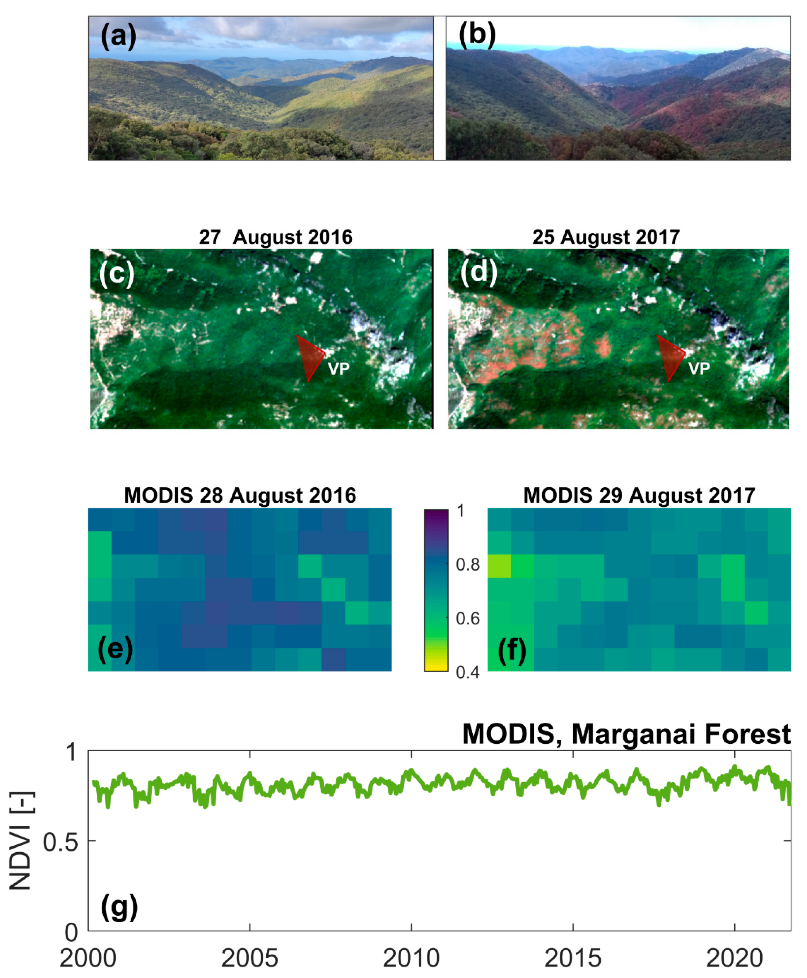
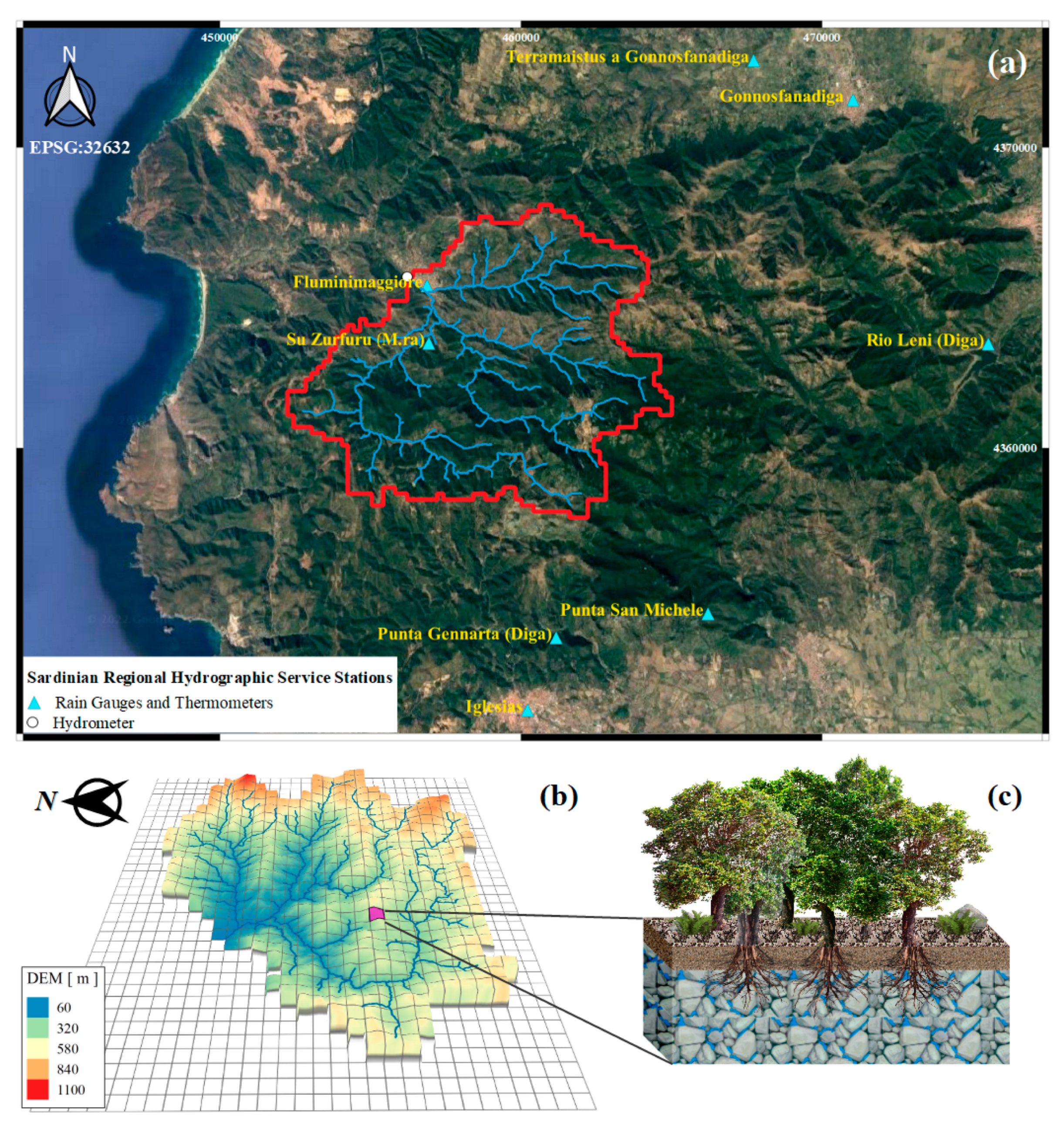
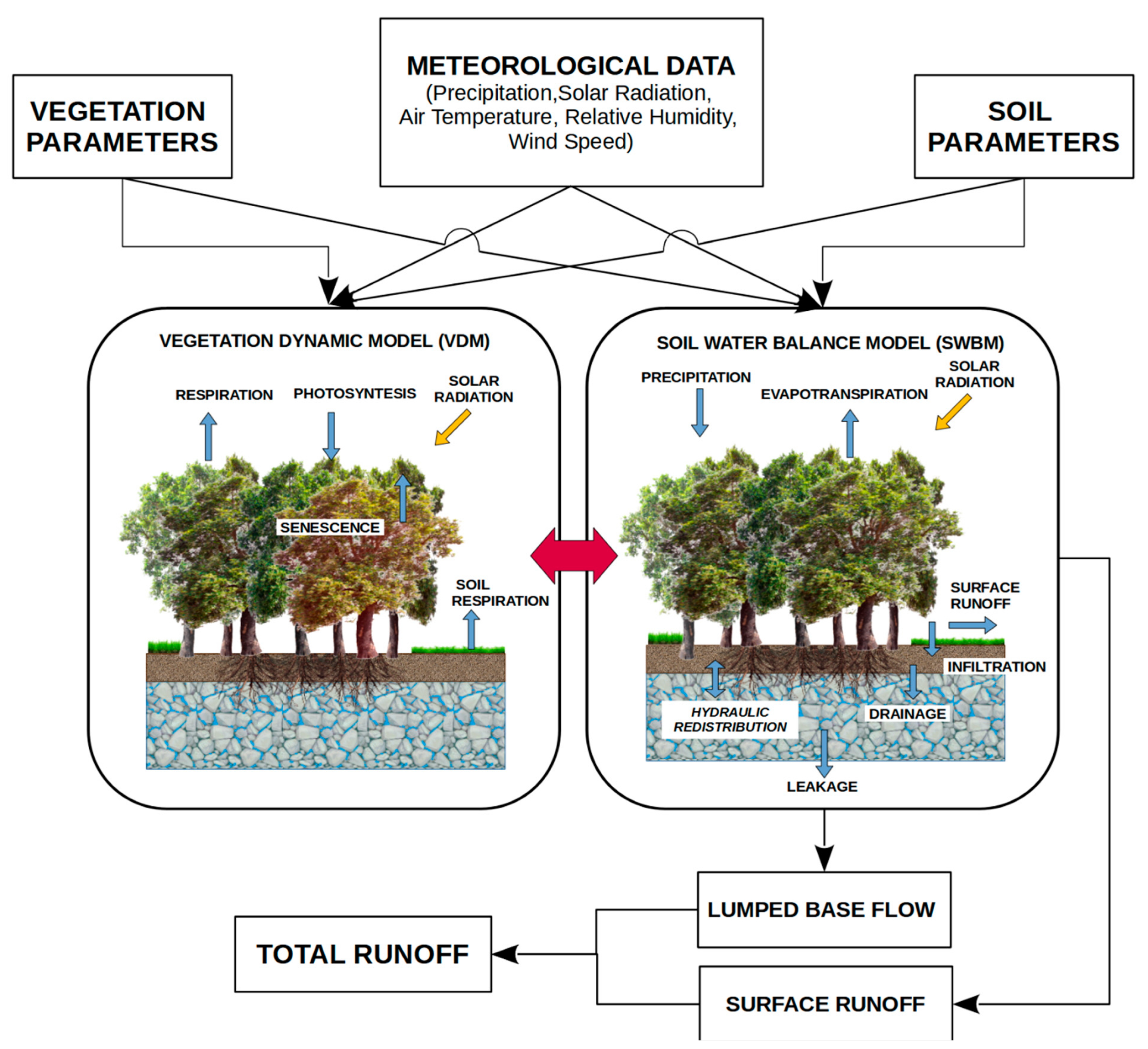
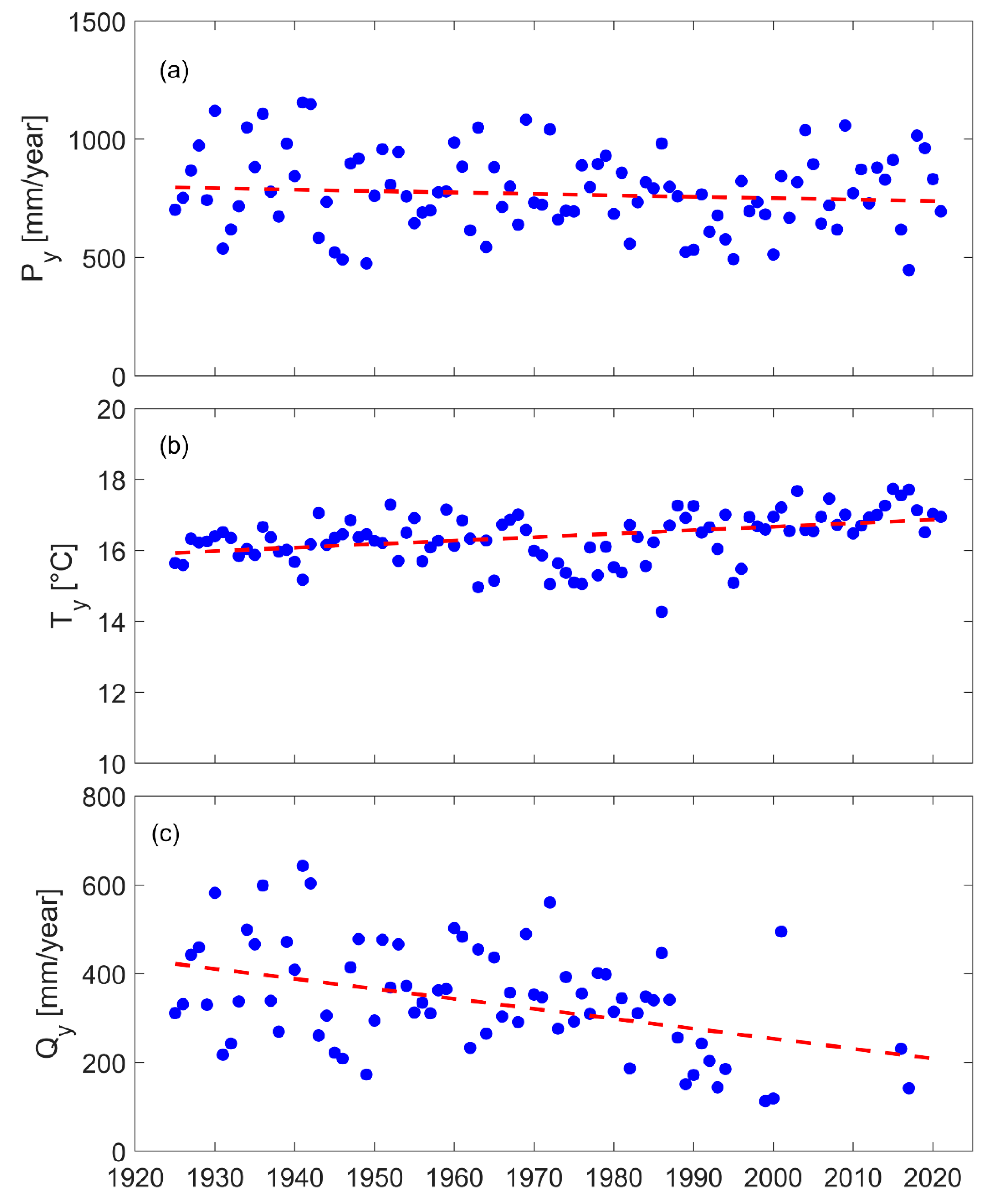
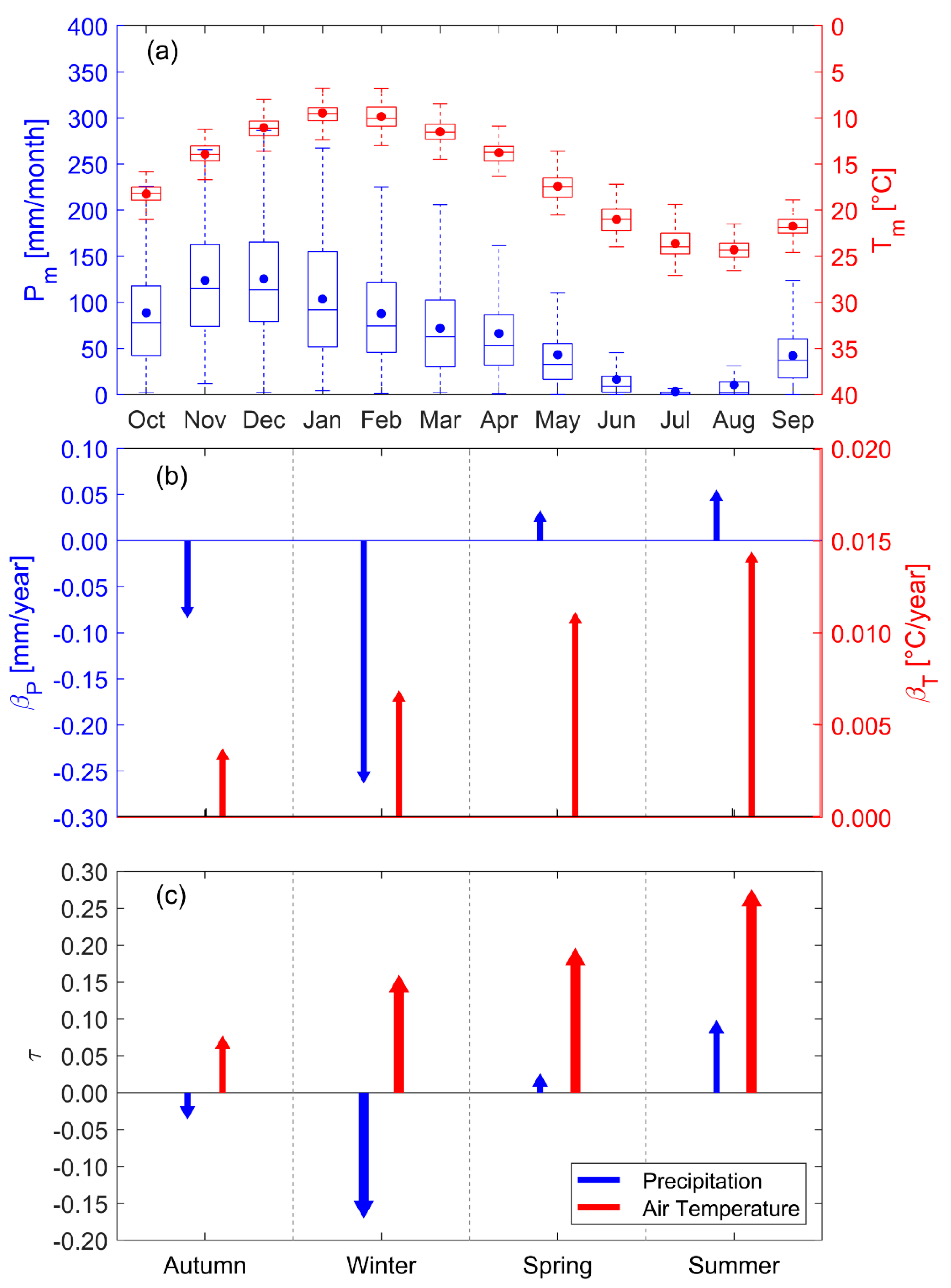
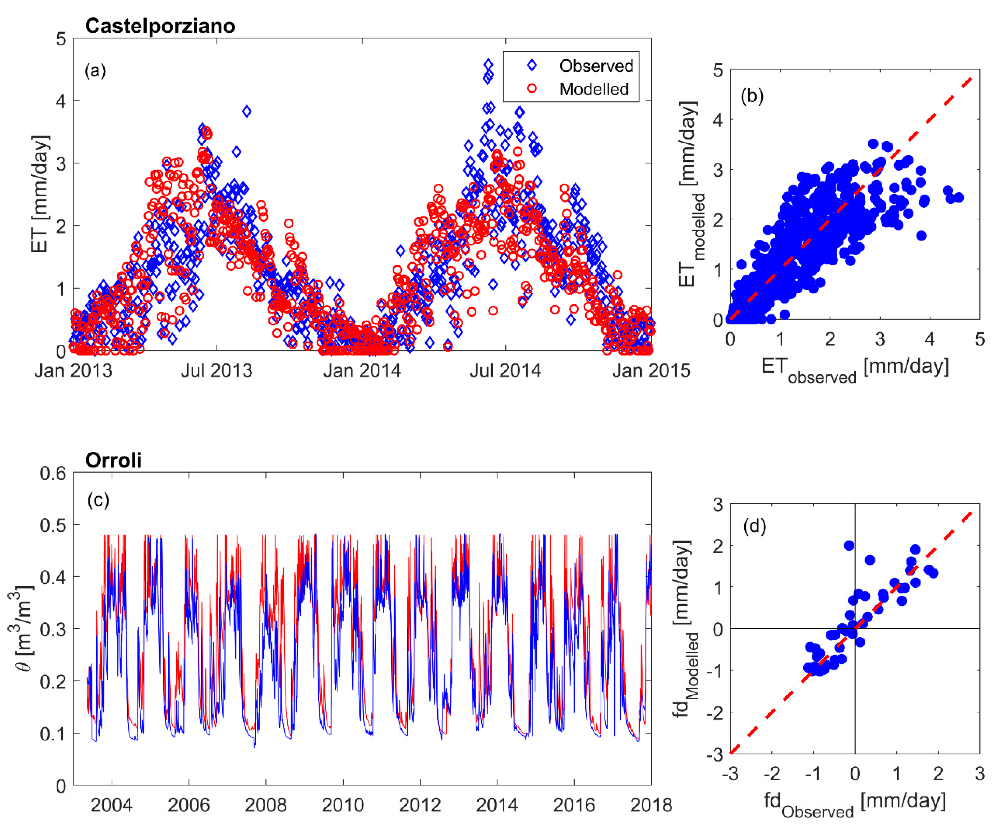
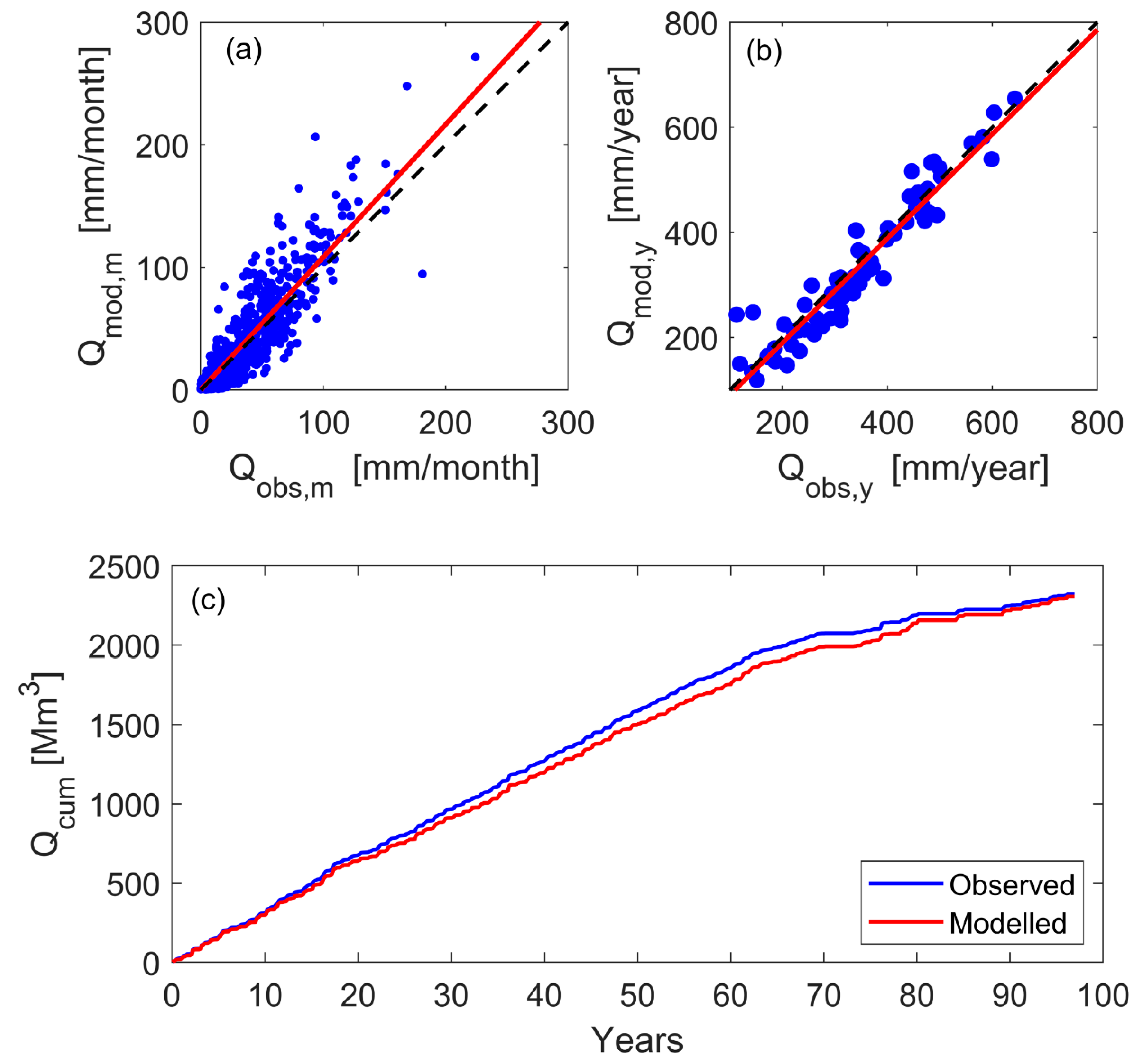
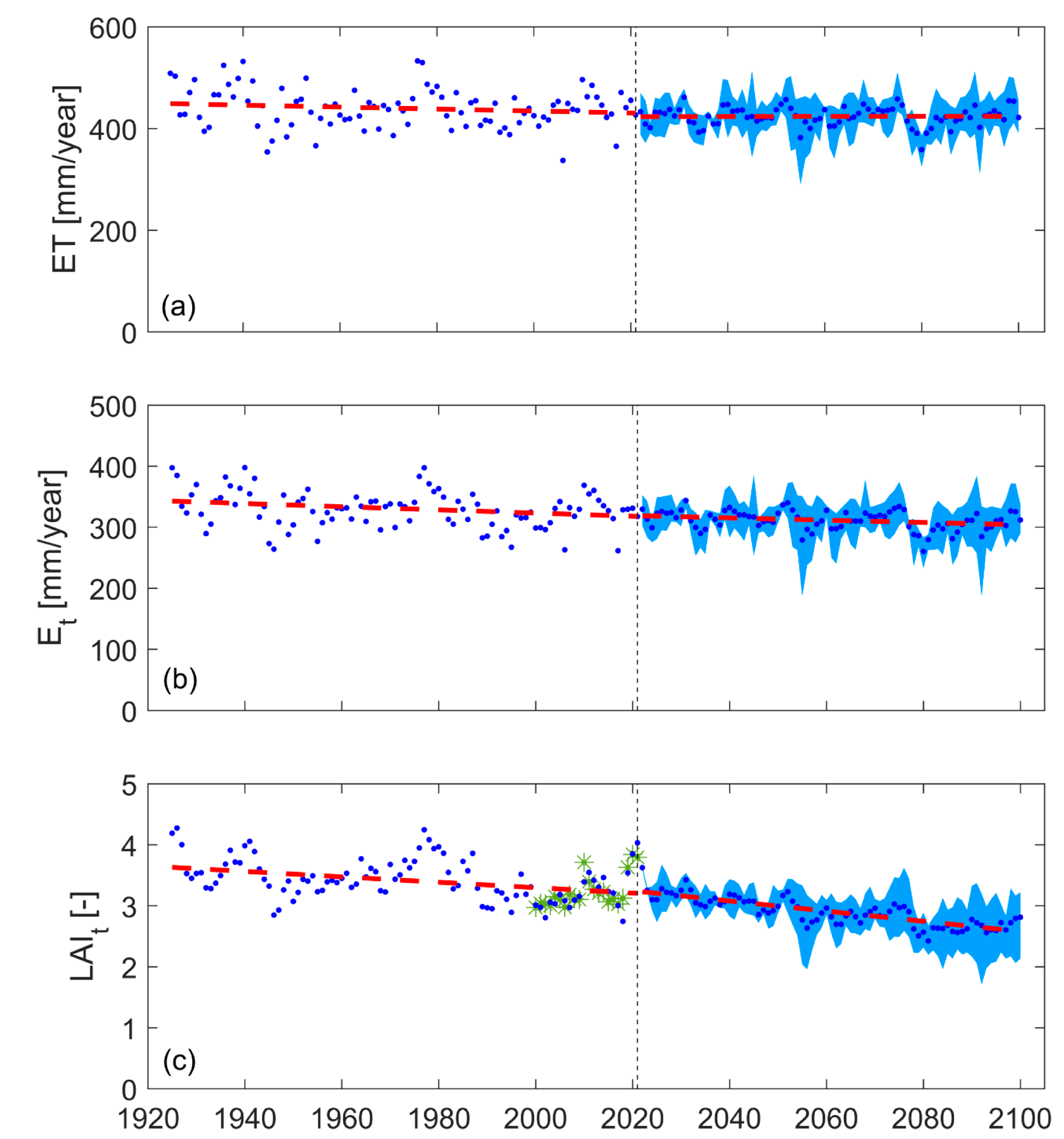
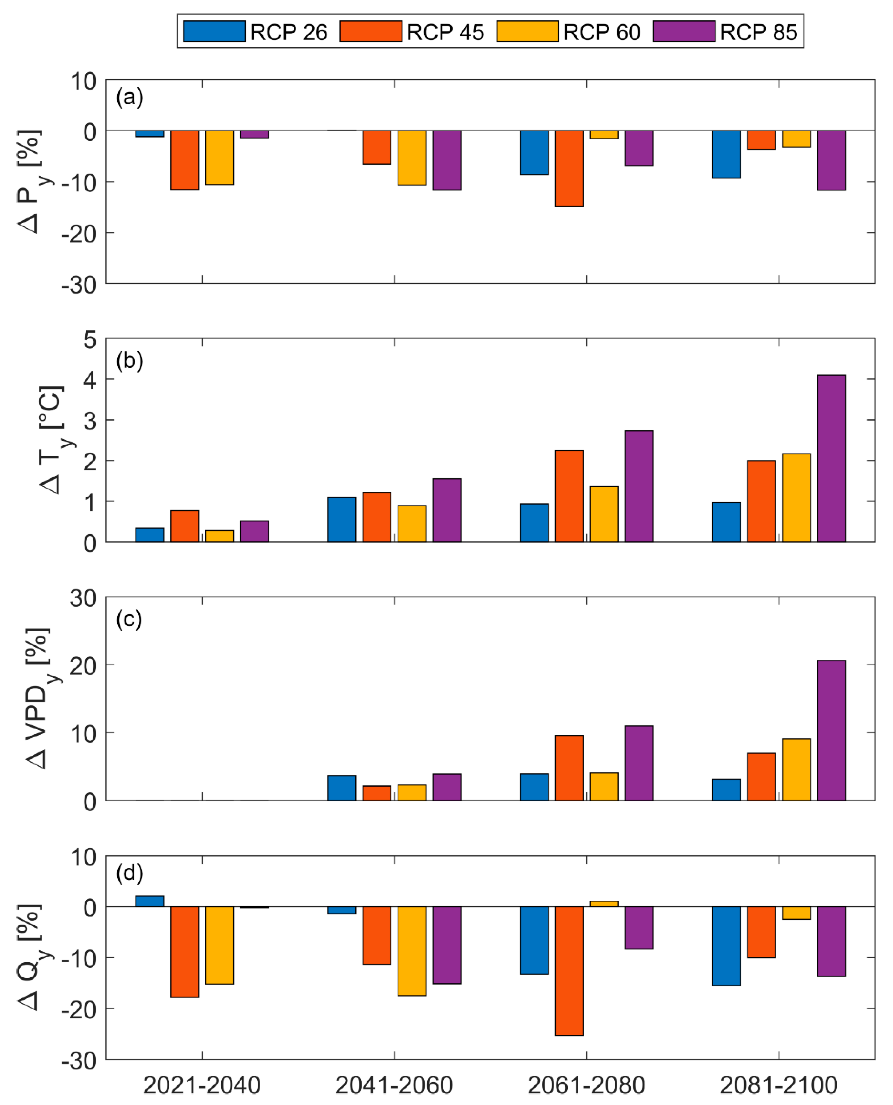
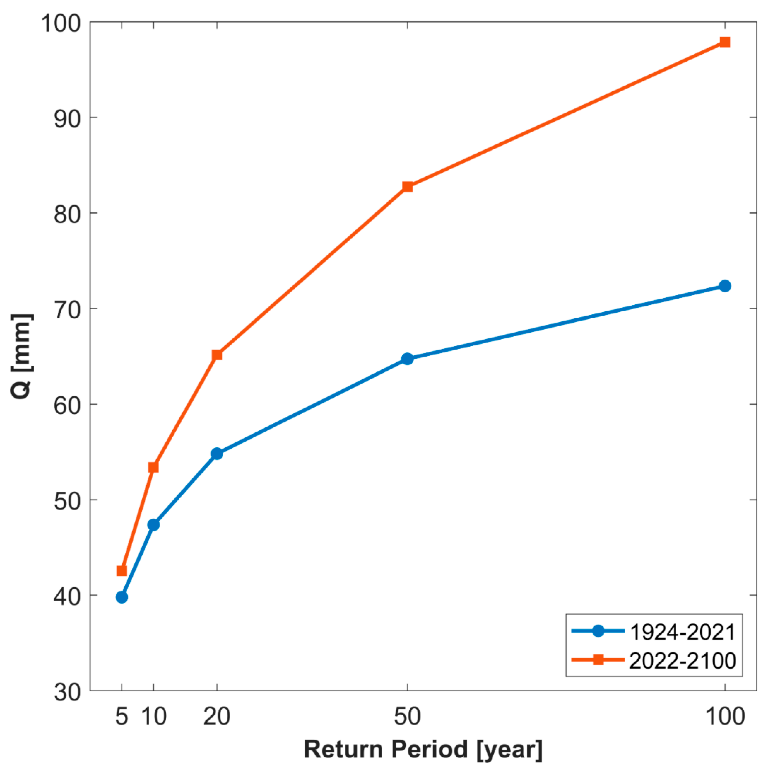
Table 1.
Model parameters of the vegetation components.
| Parameter | Description | Grass | Forest |
|---|---|---|---|
| rs,min (s m−1) | Minimum stomatal resistance | 150 | 290 |
| θwp (-) | Wilting point | 0.08 | 0.05 |
| θlim (-) | Limiting soil moisture for vegetation | 0.20 | 0.18 |
| Tmin (°K) | Minimum temperature | 279.15 | 268.15 |
| Topt (°K) | Optimal temperature | 293.15 | 288.15 |
| Tmax (°K) | Maximum temperature | 299.15 | 304.15 |
| ca (m2 gDM−1) | Specific leaf areas of the green biomass | 0.01 | 0.0065 |
| cd (m2 gDM−1) | Specific leaf areas of the dead biomass | 0.01 | 0.0062 |
| ke (-) | PAR extinction coefficient | 0.5 | 0.5 |
| ξa (-) | Parameter controlling allocation to leaves | 0.6 | 0.55 |
| ξs (-) | Parameter controlling allocation to stem | 0.1 | 0.1 |
| ξr (-) | Parameter controlling allocation to roots | 0.4 | 0.35 |
| Ω (-) | Allocation parameter | 0.8 | 0.1 |
| ma (d−1) | Maintenance respiration coefficients for aboveground biomass | 0.032 | 0.0001 |
| ga (-) | Growth respiration coefficients for aboveground biomass | 0.32 | 0.85 |
| mr (d−1) | Maintenance respiration coefficients for root biomass | 0.007 | 0.0003 |
| gr (-) | Growth respiration coefficients for root biomass | 0.1 | 0.1 |
| Q10 (-) | Temperature coefficient in the respiration process | 2.5 | 3 |
| da (d−1) | Death rate of aboveground biomass | 0.023 | 0.0019 |
| dr (d−1) | Death rate of root biomass | 0.005 | 0.0001 |
| ka (d−1) | Rate of standing biomass pushed down | 0.23 | 0.35 |
| QN (-) | Soil respiration coefficient related to temperature | 1.2 | |
| R10 (mmol CO2/m2s) | Reference respiration at 10 °C | 2.54 | |
| zom,v (m) | Vegetation momentum roughness length | 0.05 | 0.5 |
| zov,v (m) | Vegetation water vapor roughness length | zom/7.4 | zom/2.5 |
| zom,bs (m) | Bare soil momentum roughness length | 0.015 | |
| zov,bs (m) | Bare soil water vapor roughness length | zom/10 | |
Table 2.
Equations of the vegetation dynamic model components. Parameters are defined in Table 1.
Table 2.
Equations of the vegetation dynamic model components. Parameters are defined in Table 1.
| Ecophysiological Term | Equation |
|---|---|
| Photosynthesis | |
| Allocation | For woody vegetation |
| For grass | |
| Respiration | |
| Senescence | |
| Litterfall |
Table 3.
Soil-related parameters of the model.
| Parameter | Description | Mean | Range |
|---|---|---|---|
| CN | Curve Number of the Soil Conservation Service method | 89.7 | 80–99 |
| θsat,s (-) | Saturated soil moisture | 0.44 | 0.41−0.46 |
| bs (-) | Slope of the retention curve in the surface soil | 10.28 | 7.75−11.40 |
| ksat,s (m/s) | Saturated hydraulic conductivity | 2.82 × 10⁻⁷ | 10−8−10−6 |
| ds (m) | Soil layer depth | 0.36 | 0.20−0.85 |
| qsat,r (-) | Saturated rock moisture | 0.48 | 0.45−0.50 |
| br (-) | Slope of the retention curve in the fracture rock layer | 7 | |
| ksat,r (m/s) | Saturated hydraulic conductivity in the fracture rock layer | 1.41 × 10⁻⁷ | 5 × 10⁻⁹−5 × 10⁻⁷ |
| dr (m) | Fractured rock depth | 1.5 | |
Table 4.
Past mean changes (1976−2000 with 1951−1975) of annual precipitation (Py), air temperature (Ty), and predicted annual runoff (Qy), evapotranspiration (ETy), and tree LAI (LAIt,y) using observations of the Sardinian meteorological network and the HadGEM2-AO meteorological data as model input.
| ΔPy (%) | ΔTy (%) | ΔQy (%) | ΔETy (%) | ΔLAIt,y (%) | |
|---|---|---|---|---|---|
| From land-observations | −8.47 | 1.36 | −20.73 | −1.85 | −1.39 |
| HadGEM2-AO | −9.42 | 1.67 | −16.18 | −2.57 | −2.07 |
Table 5.
Results of the statistical tests (Chi-square and Kolmogorov−Smirnov tests) of the Generalized Extreme Value distribution fitting to the annual maximum daily runoff time series of the Fluminimaggiore basin for the past (1924–2021) and the future climate scenario (2022–2100), predicted using HadGEM2-AO data in the RCP 85 configuration. Statistics of the Chi-square and Kolmogorov−Smirnov tests for normality, applied to the series, have 5% significance level.
| Period | Kolmogorov–Smirnov | Χ2 |
|---|---|---|
| 1924−2021 | 0.0721 (0.1354) | 4.2951 (5.991) |
| 2022−2100 | 0.0783 (0.1505) | 5.1175 (5.991) |
Publisher’s Note: MDPI stays neutral with regard to jurisdictional claims in published maps and institutional affiliations. |
© 2022 by the authors. Licensee MDPI, Basel, Switzerland. This article is an open access article distributed under the terms and conditions of the Creative Commons Attribution (CC BY) license (https://creativecommons.org/licenses/by/4.0/).
Share and Cite
MDPI and ACS Style
Sirigu, S.; Montaldo, N. Climate Change Impacts on the Water Resources and Vegetation Dynamics of a Forested Sardinian Basin through a Distributed Ecohydrological Model. Water 2022, 14, 3078. https://doi.org/10.3390/w14193078
AMA Style
Sirigu S, Montaldo N. Climate Change Impacts on the Water Resources and Vegetation Dynamics of a Forested Sardinian Basin through a Distributed Ecohydrological Model. Water. 2022; 14(19):3078. https://doi.org/10.3390/w14193078
Chicago/Turabian StyleSirigu, Serena, and Nicola Montaldo. 2022. "Climate Change Impacts on the Water Resources and Vegetation Dynamics of a Forested Sardinian Basin through a Distributed Ecohydrological Model" Water 14, no. 19: 3078. https://doi.org/10.3390/w14193078
Note that from the first issue of 2016, this journal uses article numbers instead of page numbers. See further details here.