
Flash Flood Susceptibility Assessment and Zonation by Integrating Analytic Hierarchy Process and Frequency Ratio Model with Diverse Spatial Data

 , , , , , ,
Abstract
:1. Introduction
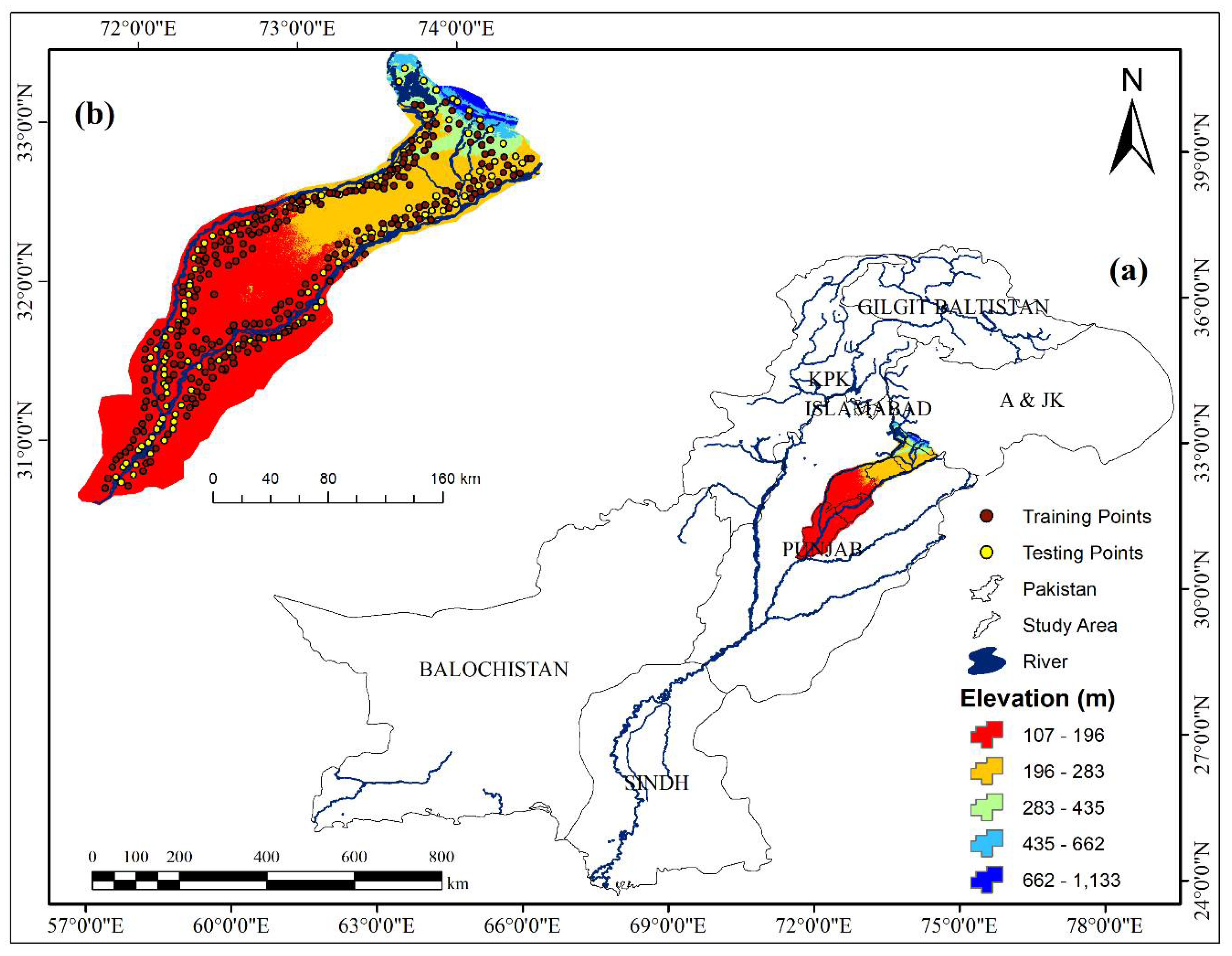
2. Study Area
3. Collection and Preparation of Data
3.1. Inventory of Flash Flood Zoning
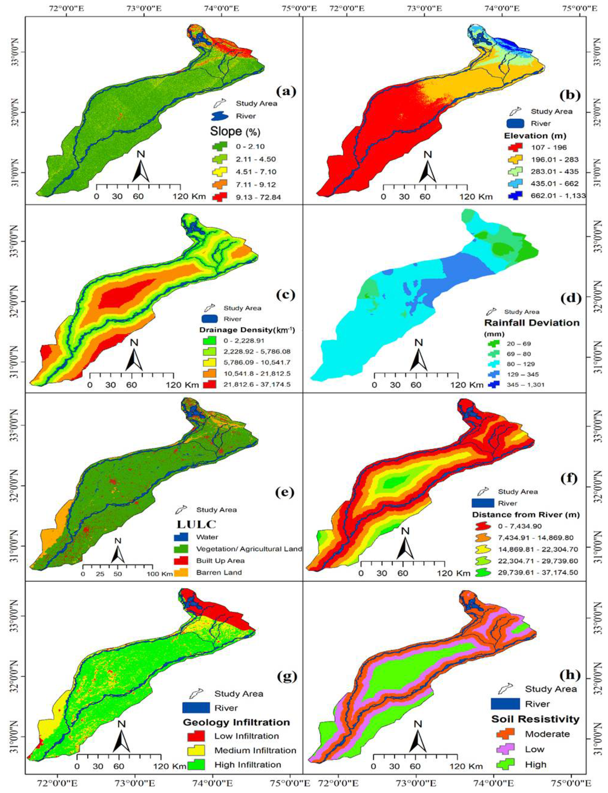
3.2. Flash Flood Conditioning Factors
3.2.1. Slope
3.2.2. Elevation
3.2.3. Drainage Density
3.2.4. Rainfall Deviation
3.2.5. Land Use and Land Cover
3.2.6. Distance from the Stream
3.2.7. Geology
3.2.8. Soil
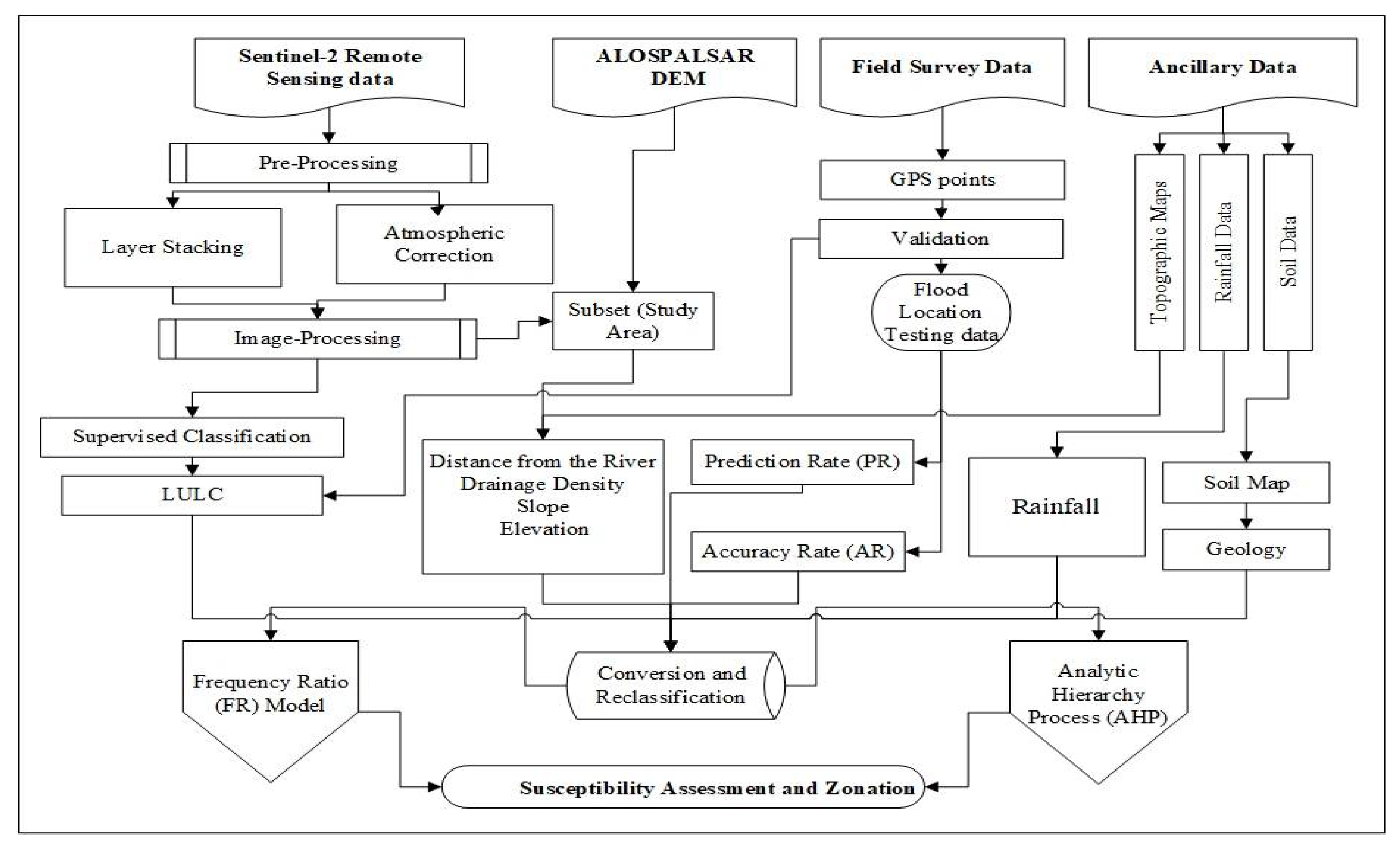
4. Methods and Methodology
4.1. Collection of Data and Its Preparation
4.2. Training and Testing Datasets’ Generation
4.3. AHP Modeling and the SFWV
4.4. FR Model and the SCWV
4.5. Validation
5. Results
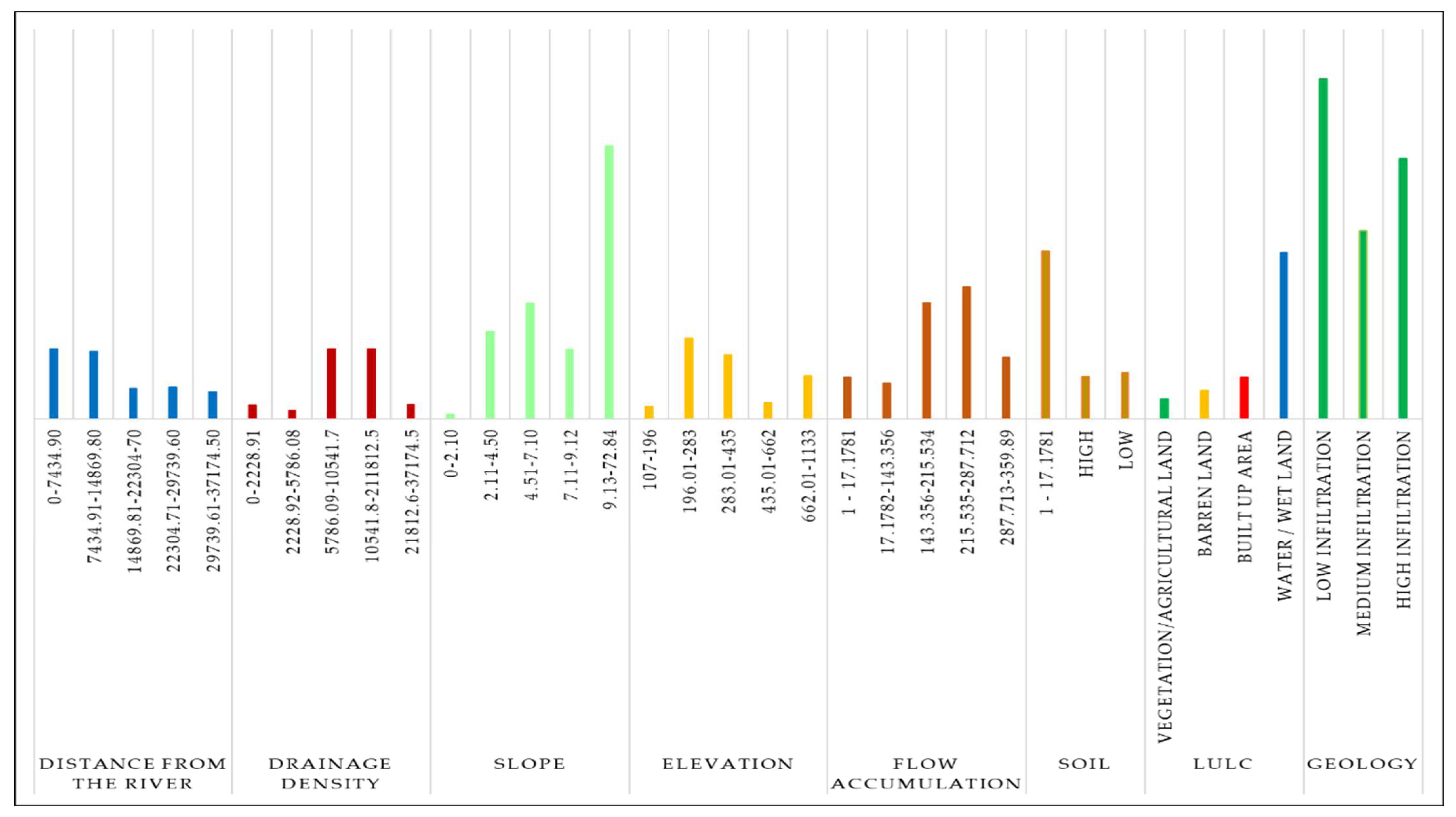
5.1. Effect Weight of Each Class of Flash Flood Susceptibility Variables Found Using the FR Method
5.2. Relationships between Flood Susceptibility and Flood-Inducing Factors
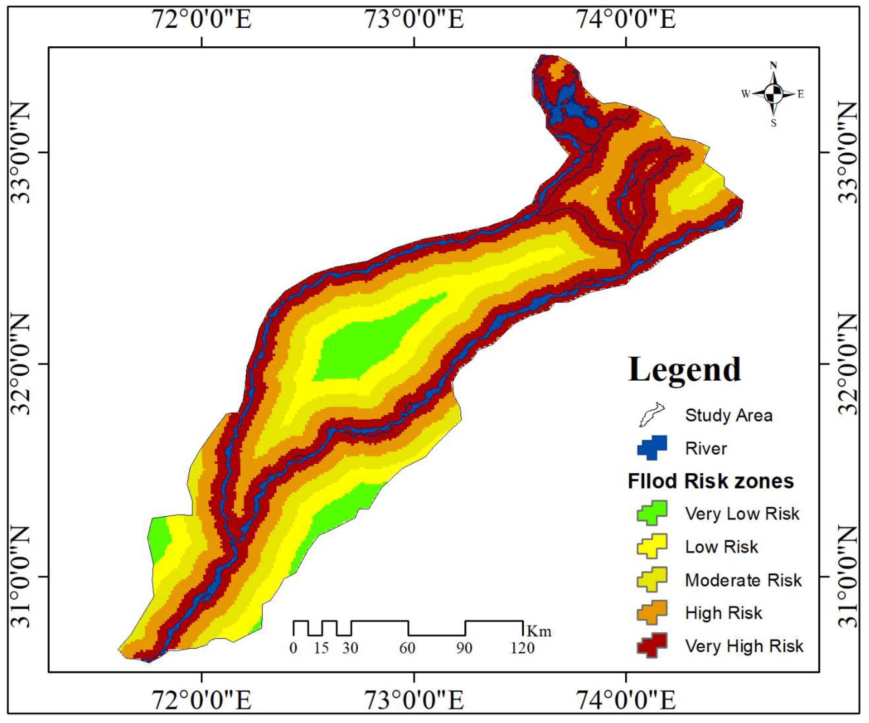
5.3. Susceptibility Mapping of Flood and Estimation of Risk Area
5.4. Validation Analysis of Risky Zone of the Study Area
6. Discussion
7. Conclusions
Author Contributions
Funding
Data Availability Statement
Acknowledgments
Conflicts of Interest
References
- Hussain, E.; Ural, S.; Malik, A.; Shan, J. Mapping pakistan 2010 floods using remote sensing data. In Proceedings of the American Society for Photogrammetry and Remote Sensing Annual Conference, Milwaukee, WI, USA, 1–5 May 2011; Volume 2011, pp. 215–222. [Google Scholar]
- Yue, Z.; Zhou, W.; Li, T. Impact of the Indian Ocean Dipole on Evolution of the Subsequent ENSO: Relative Roles of Dynamic and Thermodynamic Processes. J. Clim. 2021, 34, 3591–3607. [Google Scholar] [CrossRef]
- Quan, Q.; Gao, S.; Shang, Y.; Wang, B. Assessment of the sustainability of Gymnocypris eckloni habitat under river damming in the source region of the Yellow River. Sci. Total Environ. 2021, 778, 146312. [Google Scholar] [CrossRef] [PubMed]
- Zhang, K.; Wang, S.; Bao, H.; Zhao, X. Characteristics and influencing factors of rainfall-induced landslide and debris flow hazards in Shaanxi Province, China. Nat. Hazards Earth Syst. Sci. 2019, 19, 93–105. [Google Scholar] [CrossRef]
- Wang, S.; Zhang, K.; Chao, L.; Li, D.; Tian, X.; Bao, H.; Chen, G.; Xia, Y. Exploring the utility of radar and satellite-sensed precipitation and their dynamic bias correction for integrated prediction of flood and landslide hazards. J. Hydrol. 2021, 603, 126964. [Google Scholar] [CrossRef]
- Wahla, S.S.; Kazmi, J.; Sharifi, A.; Shirazi, S.; Tariq, A.; Smith, H.J. Assessing Spatio-temporal mapping and monitoring of climatic Variability using SPEI and RF machine learning models. Geocarto Int. 2022, 1–22. [Google Scholar] [CrossRef]
- Dai, J.; Feng, H.; Shi, K.; Ma, X.; Yan, Y.; Ye, L.; Xia, Y. Electrochemical degradation of antibiotic enoxacin using a novel PbO2 electrode with a graphene nanoplatelets inter-layer: Characteristics, efficiency and mechanism. Chemosphere 2022, 307, 135833. [Google Scholar] [CrossRef] [PubMed]
- Liu, E.; Chen, S.; Yan, D.; Deng, Y.; Wang, H.; Jing, Z.; Pan, S. Detrital zircon geochronology and heavy mineral composition constraints on provenance evolution in the western Pearl River Mouth basin, northern south China sea: A source to sink approach. Mar. Pet. Geol. 2022, 145, 105884. [Google Scholar] [CrossRef]
- Chen, X.; Quan, Q.; Zhang, K.; Wei, J. Spatiotemporal characteristics and attribution of dry/wet conditions in the Weihe River Basin within a typical monsoon transition zone of East Asia over the recent 547 years. Environ. Model. Softw. 2021, 143, 105116. [Google Scholar] [CrossRef]
- Huang, Y.; Bárdossy, A.; Zhang, K. Sensitivity of hydrological models to temporal and spatial resolutions of rainfall data. Hydrol. Earth Syst. Sci. 2019, 23, 2647–2663. [Google Scholar] [CrossRef]
- Tariq, A.; Riaz, I.; Ahmad, Z.; Yang, B.; Amin, M.; Kausar, R.; Andleeb, S.; Farooqi, M.A.; Rafiq, M. Land surface temperature relation with normalized satellite indices for the estimation of spatio-temporal trends in temperature among various land use land cover classes of an arid Potohar region using Landsat data. Environ. Earth Sci. 2019, 79, 40. [Google Scholar] [CrossRef]
- Waqas, H.; Lu, L.; Tariq, A.; Li, Q.; Baqa, M.; Xing, J.; Sajjad, A. Flash Flood Susceptibility Assessment and Zonation Using an Integrating Analytic Hierarchy Process and Frequency Ratio Model for the Chitral District, Khyber Pakhtunkhwa, Pakistan. Water 2021, 13, 1650. [Google Scholar] [CrossRef]
- Tariq, A.; Mumtaz, F.; Zeng, X.; Baloch, M.Y.J.; Moazzam, M.F.U. Spatio-temporal variation of seasonal heat islands mapping of Pakistan during 2000–2019, using day-time and night-time land surface temperatures MODIS and meteorological stations data. Remote Sens. Appl. Soc. Environ. 2022, 27, 100779. [Google Scholar] [CrossRef]
- Zhu, Z.; Wu, Y.; Liang, Z. Mining-Induced Stress and Ground Pressure Behavior Characteristics in Mining a Thick Coal Seam With Hard Roofs. Front. Earth Sci. 2022, 10, 843191. [Google Scholar] [CrossRef]
- Guo, Y.; Yang, Y.; Kong, Z.; He, J. Development of Similar Materials for Liquid-Solid Coupling and Its Application in Water Outburst and Mud Outburst Model Test of Deep Tunnel. Geofluids 2022, 2022, 8784398. [Google Scholar] [CrossRef]
- Liu, Y.; Zhang, Z.; Liu, X.; Wang, L.; Xia, X. Efficient image segmentation based on deep learning for mineral image classification. Adv. Powder Technol. 2021, 32, 3885–3903. [Google Scholar] [CrossRef]
- Chen, Z.; Liu, Z.; Yin, L.; Zheng, W. Statistical analysis of regional air temperature characteristics before and after dam construction. Urban Clim. 2022, 41, 101085. [Google Scholar] [CrossRef]
- Yin, L.; Wang, L.; Keim, B.D.; Konsoer, K.; Zheng, W. Wavelet Analysis of Dam Injection and Discharge in Three Gorges Dam and Reservoir with Precipitation and River Discharge. Water 2022, 14, 567. [Google Scholar] [CrossRef]
- Yin, L.; Wang, L.; Zheng, W.; Ge, L.; Tian, J.; Liu, Y.; Yang, B.; Liu, S. Evaluation of Empirical Atmospheric Models Using Swarm-C Satellite Data. Atmosphere 2022, 13, 294. [Google Scholar] [CrossRef]
- Zhang, X.; Ma, F.; Yin, S.; Wallace, C.D.; Soltanian, M.R.; Dai, Z.; Ritzi, R.W.; Ma, Z.; Zhan, C.; Lü, X. Application of upscaling methods for fluid flow and mass transport in multi-scale heterogeneous media: A critical review. Appl. Energy 2021, 303, 117603. [Google Scholar] [CrossRef]
- Zhan, C.; Dai, Z.; Samper, J.; Yin, S.; Ershadnia, R.; Zhang, X.; Wang, Y.; Yang, Z.; Luan, X.; Soltanian, M.R. An integrated inversion framework for heterogeneous aquifer structure identification with single-sample generative adversarial network. J. Hydrol. 2022, 610. [Google Scholar] [CrossRef]
- Avand, M.; Moradi, H.; Lasboyee, M.R. Spatial modeling of flood probability using geo-environmental variables and machine learning models, case study: Tajan watershed, Iran. Adv. Space Res. 2021, 67, 3169–3186. [Google Scholar] [CrossRef]
- Thomas, V. Climate Change and Natural Disasters; Taylor & Francis Group: New York, NY, USA, 2017; Volume 8, pp. 81–94. [Google Scholar] [CrossRef]
- Tehrany, M.S.; Lee, M.J.; Pradhan, B.; Jebur, M.N.; Lee, S. Flood susceptibility mapping using integrated bivariate and multivariate statistical models. Environ. Earth Sci. 2014, 72, 4001–4015. [Google Scholar] [CrossRef]
- Costache, R.; Pham, Q.B.; Arabameri, A.; Diaconu, D.C.; Costache, I.; Crăciun, A.; Ciobotaru, N.; Pandey, M.; Arora, A.; Ali, S.A.; et al. Flash-flood propagation susceptibility estimation using weights of evidence and their novel ensembles with multicriteria decision making and machine learning. Geocarto Int. 2021, 1–33. [Google Scholar] [CrossRef]
- Khatoon, R.; Hussain, I.; Anwar, M.; Nawaz, M.A. Diet selection of snow leopard (Panthera uncia) in Chitral, Pakistan. Turk. J. Zool. 2017, 41, 914–923. [Google Scholar] [CrossRef]
- Huang, S.; Liu, C. A computational framework for fluid–structure interaction with applications on stability evaluation of breakwater under combined tsunami–earthquake activity. Comput. Civ. Infrastruct. Eng. 2022. [Google Scholar] [CrossRef]
- Zhou, G.; Long, S.; Xu, J.; Zhou, X.; Song, B.; Deng, R.; Wang, C. Comparison Analysis of Five Waveform Decomposition Algorithms for the Airborne LiDAR Echo Signal. IEEE J. Sel. Top. Appl. Earth Obs. Remote Sens. 2021, 14, 7869–7880. [Google Scholar] [CrossRef]
- Zhou, G.; Zhang, R.; Huang, S. Generalized Buffering Algorithm. IEEE Access 2021, 9, 27140–27157. [Google Scholar] [CrossRef]
- Wang, Q.; Zhou, G.; Song, R.; Xie, Y.; Luo, M.; Yue, T. Continuous space ant colony algorithm for automatic selection of orthophoto mosaic seamline network. ISPRS J. Photogramm. Remote Sens. 2022, 186, 201–217. [Google Scholar] [CrossRef]
- Wang, P.; Wang, L.; Leung, H.; Zhang, G. Super-Resolution Mapping Based on Spatial–Spectral Correlation for Spectral Imagery. IEEE Trans. Geosci. Remote Sens. 2020, 59, 2256–2268. [Google Scholar] [CrossRef]
- Tian, H.; Qin, Y.; Niu, Z.; Wang, L.; Ge, S. Summer Maize Mapping by Compositing Time Series Sentinel-1A Imagery Based on Crop Growth Cycles. J. Indian Soc. Remote Sens. 2021, 49, 2863–2874. [Google Scholar] [CrossRef]
- Tian, H.; Wang, Y.; Chen, T.; Zhang, L.; Qin, Y. Early-Season Mapping of Winter Crops Using Sentinel-2 Optical Imagery. Remote Sens. 2021, 13, 3822. [Google Scholar] [CrossRef]
- Tian, H.F.; Huang, N.; Niu, Z.; Qin, Y.C.; Pei, J.; Wang, J. Mapping Winter Crops in China with Multi-Source Satellite Imagery and Phenology-Based Algorithm. Remote Sens. 2019, 11, 820. [Google Scholar] [CrossRef]
- Avand, M.; Moradi, H.R.; Ramazanzadeh Lasboyee, M. Spatial Prediction of Future Flood Risk: An Approach to the Effects of Climate Change. Geoscience 2021, 11, 25. [Google Scholar] [CrossRef]
- Tian, H.; Pei, J.; Huang, J.; Li, X.; Wang, J.; Zhou, B.; Qin, Y.; Wang, L. Garlic and Winter Wheat Identification Based on Active and Passive Satellite Imagery and the Google Earth Engine in Northern China. Remote Sens. 2020, 12, 3539. [Google Scholar] [CrossRef]
- Luan, D.; Liu, A.; Wang, X.; Xie, Y.; Wu, Z. Robust Two-Stage Location Allocation for Emergency Temporary Blood Supply in Postdisaster. Discret. Dyn. Nat. Soc. 2022, 2022, 6184170. [Google Scholar] [CrossRef]
- Chen, J.; Du, L.; Guo, Y. Label constrained convolutional factor analysis for classification with limited training samples. Inf. Sci. 2020, 544, 372–394. [Google Scholar] [CrossRef]
- Tariq, A.; Shu, H. CA-Markov Chain Analysis of Seasonal Land Surface Temperature and Land Use Landcover Change Using Optical Multi-Temporal Satellite Data of Faisalabad, Pakistan. Remote Sens. 2020, 12, 3402. [Google Scholar] [CrossRef]
- Bui, D.T.; Tsangaratos, P.; Ngo, P.-T.T.; Pham, T.D.; Pham, B.T. Flash flood susceptibility modeling using an optimized fuzzy rule based feature selection technique and tree based ensemble methods. Sci. Total Environ. 2019, 668, 1038–1054. [Google Scholar] [CrossRef]
- Hoang, L.P.; Biesbroek, R.; Tri, V.P.D.; Kummu, M.; van Vliet, M.T.H.; Leemans, R.; Kabat, P.; Ludwig, F. Managing flood risks in the Mekong Delta: How to address emerging challenges under climate change and socioeconomic developments. Ambio 2018, 47, 635–649. [Google Scholar] [CrossRef] [Green Version]
- Liu, M.; Chen, N.; Zhang, Y.; Deng, M. Glacial Lake Inventory and Lake Outburst Flood/Debris Flow Hazard Assessment after the Gorkha Earthquake in the Bhote Koshi Basin. Water 2020, 12, 464. [Google Scholar] [CrossRef]
- Kirkby, M.; Bracken, L.; Reaney, S. The influence of land use, soils and topography on the delivery of hillslope runoff to channels in SE Spain. Earth Surf. Process. Landf. 2002, 27, 1459–1473. [Google Scholar] [CrossRef]
- European Environmental Agency. Mapping the Impacts of Natural Hazards and Technological Accidents in Europe: An Overview of the Last Decade; Publications Office of the European Union: Luxembourg, 2010; ISBN 978-92-9213-168-5. [Google Scholar]
- Aoki, K.; Uehara, M.; Kato, C.; Hirahara, H. Evaluation of Rugby Players’ Psychological-Competitive Ability by Utilizing the Analytic Hierarchy Process. Open J. Soc. Sci. 2016, 4, 103–117. [Google Scholar] [CrossRef]
- Alexakis, D.D.; Sarris, A. Integrated GIS and remote sensing analysis for landfill sitting in Western Crete, Greece. Environ. Earth Sci. 2013, 72, 467–482. [Google Scholar] [CrossRef]
- Ahmad, D.; Afzal, M. Flood hazards and factors influencing household flood perception and mitigation strategies in Pakistan. Environ. Sci. Pollut. Res. 2020, 27, 15375–15387. [Google Scholar] [CrossRef] [PubMed]
- Li, Y.; Du, L.; Wei, D. Multiscale CNN Based on Component Analysis for SAR ATR. IEEE Trans. Geosci. Remote Sens. 2021, 60, 1–12. [Google Scholar] [CrossRef]
- Zhao, M.; Zhou, Y.; Li, X.; Cheng, W.; Zhou, C.; Ma, T.; Li, M.; Huang, K. Mapping urban dynamics (1992–2018) in Southeast Asia using consistent nighttime light data from DMSP and VIIRS. Remote Sens. Environ. 2020, 248, 111980. [Google Scholar] [CrossRef]
- Zhao, M.; Zhou, Y.; Li, X.; Zhou, C.; Cheng, W.; Li, M.; Huang, K. Building a Series of Consistent Night-Time Light Data (1992–2018) in Southeast Asia by Integrating DMSP-OLS and NPP-VIIRS. IEEE Trans. Geosci. Remote Sens. 2019, 58, 1843–1856. [Google Scholar] [CrossRef]
- Muhammad Ishaq, I. ullah Political/Power Structure and Vulnerability to Natural Disaster in North Western Pakistan. Res. J. Soc. Sci. Econ. Rev. 2020, 1, 389–400. [Google Scholar]
- Dewan, T.H. Societal impacts and vulnerability to floods in Bangladesh and Nepal. Weather Clim. Extrem. 2014, 7, 36–42. [Google Scholar] [CrossRef]
- Soriano, I.R.; Prot, J.C.; Matias, D.M. Expression of Tolerance for Meloidogyne graminicola in Rice Cultivars as Affected by Soil Type and Flooding. J. Nematol. 2000, 32, 309–317. [Google Scholar]
- Costache, R.; Tin, T.T.; Arabameri, A.; Crăciun, A.; Ajin, R.; Costache, I.; Islam, A.R.M.T.; Abba, S.; Sahana, M.; Avand, M.; et al. Flash-flood hazard using deep learning based on H2O R package and fuzzy-multicriteria decision-making analysis. J. Hydrol. 2022, 609, 127747. [Google Scholar] [CrossRef]
- Ouma, Y.O.; Tateishi, R. Urban Flood Vulnerability and Risk Mapping Using Integrated Multi-Parametric AHP and GIS: Methodological Overview and Case Study Assessment. Water 2014, 6, 1515–1545. [Google Scholar] [CrossRef]
- Ali, S.A.; Khatun, R.; Ahmad, A.; Ahmad, S.N. Application of GIS-based analytic hierarchy process and frequency ratio model to flood vulnerable mapping and risk area estimation at Sundarban region, India. Model. Earth Syst. Environ. 2019, 5, 1083–1102. [Google Scholar] [CrossRef]
- Pradhan, B.; Chaudhari, A.; Adinarayana, J.; Buchroithner, M.F. Soil erosion assessment and its correlation with landslide events using remote sensing data and GIS: A case study at Penang Island, Malaysia. Environ. Monit. Assess. 2011, 184, 715–727. [Google Scholar] [CrossRef] [PubMed]
- Strahler, A.N. Dynamic basis of geomorphology. Bull. Geol. Am. 1952, 63, 923–939. [Google Scholar] [CrossRef]
- Ghezelsofloo, A.A.; Hajibigloo, M. Application of Flood Hazard Potential Zoning by using AHP Algorithm. Civ. Eng. Res. J. 2020, 9, 150–159. [Google Scholar] [CrossRef]
- Pimentel, S.; Flowers, G.E. A numerical study of hydrologically driven glacier dynamics and subglacial flooding. Proc. R. Soc. A Math. Phys. Eng. Sci. 2010, 467, 537–558. [Google Scholar] [CrossRef]
- Khan, B.; Iqbal, M.J.; Yosufzai, M.A.K. Flood risk assessment of River Indus of Pakistan. Arab. J. Geosci. 2010, 4, 115–122. [Google Scholar] [CrossRef]
- Ashraf, M.; Bhatti, M.T.; Shakir, A.S. River bank erosion and channel evolution in sand-bed braided reach of River Chenab: Role of floods during different flow regimes. Arab. J. Geosci. 2016, 9, 140. [Google Scholar] [CrossRef]
- Yariyan, P.; Avand, M.; Abbaspour, R.A.; Torabi Haghighi, A.; Costache, R.; Ghorbanzadeh, O.; Janizadeh, S.; Blaschke, T. Flood susceptibility mapping using an improved analytic network process with statistical models. Geomat. Nat. Hazards Risk 2020, 11, 2282–2314. [Google Scholar] [CrossRef]
- Talukdar, S.; Ghose, B.; Shahfahad; Salam, R.; Mahato, S.; Pham, Q.B.; Linh, N.T.T.; Costache, R.; Avand, M. Flood susceptibility modeling in Teesta River basin, Bangladesh using novel ensembles of bagging algorithms. Stoch. Hydrol. Hydraul. 2020, 34, 2277–2300. [Google Scholar] [CrossRef]
- Avand, M.; Kuriqi, A.; Khazaei, M.; Ghorbanzadeh, O. DEM resolution effects on machine learning performance for flood probability mapping. J. Hydro-Environ. Res. 2021, 40, 1–16. [Google Scholar] [CrossRef]
- Elkhrachy, I. Vertical accuracy assessment for SRTM and ASTER Digital Elevation Models: A case study of Najran city, Saudi Arabia. Ain Shams Eng. J. 2018, 9, 1807–1817. [Google Scholar] [CrossRef]
- Giordan, D.; Notti, D.; Zucca, F.; Pepe, A.; Villa, A.; Calò, F.; Pepe, A.; Dutto, F.; Pari, P.; Baldo, M.; et al. Low cost, multiscale and multi-sensor application for flooded area mapping Low Strain rates area monitoring with AInSAR and GPS View project alpsmotion View project Low cost, multiscale and multi-sensor application for flooded area mapping. Nat. Hazards Earth Syst. Sci. 2018, 18, 1493–1516. [Google Scholar] [CrossRef]
- Samanta, S.; Kumar Pal, D.; Palsamanta, B. Flood susceptibility analysis through remote sensing, GIS and frequency ratio model. Appl. Water Sci. 2018, 8, 66. [Google Scholar] [CrossRef]
- Atif, I.; Mahboob, M.A.; Waheed, A. Spatio-Temporal Mapping and Multi-Sector Damage Assessment of 2014 Flood in Pakistan using Remote Sensing and GIS. Indian J. Sci. Technol. 2016, 8, 1–18. [Google Scholar] [CrossRef]
- Sajjad, A.; Lu, J.Z.; Chen, X.L.; Chisenga, C.; Mahmood, S. The riverine flood catastrophe in August 2010 in south Punjab, Pakistan: Potential causes, extent and damage assessment. Appl. Ecol. Environ. Res. 2019, 17, 14121–14142. [Google Scholar] [CrossRef]
- Samboko, H.T.; Abas, I.; Luxemburg, W.M.J.; Savenije, H.H.G.; Makurira, H.; Banda, K.; Winsemius, H.C. Evaluation and improvement of remote sensing-based methods for river flow management. Phys. Chem. Earth 2020, 117, 102839. [Google Scholar] [CrossRef]
- Zhao, G.; Pang, B.; Xu, Z.; Peng, D.; Xu, L. Assessment of urban flood susceptibility using semi-supervised machine learning model. Sci. Total Environ. 2019, 659, 940–949. [Google Scholar] [CrossRef]
- Markantonis, V.; Meyer, V.; Lienhoop, N. Evaluation of the environmental impacts of extreme floods in the Evros River basin using Contingent Valuation Method. Nat. Hazards 2013, 69, 1535–1549. [Google Scholar] [CrossRef]
- Saaty, T.L. A scaling method for priorities in hierarchical structures. J. Math. Psychol. 1977, 15, 234–281. [Google Scholar] [CrossRef]
- Le, L.M.; Ly, H.B.; Pham, B.T.; Le, V.M.; Pham, T.A.; Nguyen, D.H.; Tran, X.T.; Le, T.T. Hybrid artificial intelligence approaches for predicting buckling damage of steel columns under axial compression. Materials 2019, 12, 1670. [Google Scholar] [CrossRef] [PubMed]
- Stedinger, J.R.; Vogel, R.M.; Foufoula-Georgiou, E. Frequency Analysis of Extreme Events. Handb. Hydrol. 1993, 18, 1. [Google Scholar]
- Ullah, K.; Zhang, J. GIS-based flood hazard mapping using relative frequency ratio method: A case study of panjkora river basin, eastern Hindu Kush, Pakistan. PLoS ONE 2020, 15, e0229153. [Google Scholar] [CrossRef]
- Jung, Y.; Merwade, V.; Yeo, K.; Shin, Y.; Lee, S.O. An approach using a 1D hydraulic model, landsat imaging and generalized likelihood uncertainty estimation for an approximation of flood discharge. Water 2013, 5, 1598–1621. [Google Scholar] [CrossRef]
- Rahman, M.; Ningsheng, C.; Mahmud, G.I.; Islam, M.M.; Pourghasemi, H.R.; Ahmad, H.; Habumugisha, J.M.; Washakh, R.M.A.; Alam, M.; Liu, E.; et al. Flooding and its relationship with land cover change, population growth, and road density. Geosci. Front. 2021, 12, 101224. [Google Scholar] [CrossRef]
- Das, S. Geospatial mapping of flood susceptibility and hydro-geomorphic response to the floods in Ulhas basin, India. Remote Sens. Appl. Soc. Environ. 2019, 14, 60–74. [Google Scholar] [CrossRef]
- Yesilnacar, E.; Topal, T. Landslide susceptibility mapping: A comparison of logistic regression and neural networks methods in a medium scale study, Hendek region (Turkey). Eng. Geol. 2005, 79, 251–266. [Google Scholar] [CrossRef]
- Duc, T.T. Using Gis and Ahp Technique for Land-Use Suitability Analysis. Int. Symp. Geoinform. Spat. Infrastruct. Dev. Earth Allied Sci. 2006, 1–6. [Google Scholar]
- Bozdağ, A.; Yavuz, F.; Günay, A.S. AHP and GIS based land suitability analysis for Cihanbeyli (Turkey) County. Environ. Earth Sci. 2016, 75, 813. [Google Scholar] [CrossRef]
- Kayastha, P.; Dhital, M.R.; De Smedt, F. Application of the analytical hierarchy process (AHP) for landslide susceptibility mapping: A case study from the Tinau watershed, west Nepal. Comput. Geosci. 2013, 52, 398–408. [Google Scholar] [CrossRef]
- Siddayao, G.P.; Valdez, S.E.; Fernandez, P.L. Analytic Hierarchy Process (AHP) in Spatial Modeling for Floodplain Risk Assessment. Int. J. Mach. Learn. Comput. 2014, 4, 450–457. [Google Scholar] [CrossRef]
- Mondal, S.; Maiti, R. Integrating the Analytical Hierarchy Process (AHP) and the frequency ratio (FR) model in landslide susceptibility mapping of Shiv-khola watershed, Darjeeling Himalaya. Int. J. Disaster Risk Sci. 2013, 4, 200–212. [Google Scholar] [CrossRef] [Green Version]
- Khosravi, K.; Nohani, E.; Maroufinia, E.; Pourghasemi, H.R. A GIS-based flood susceptibility assessment and its mapping in Iran: A comparison between frequency ratio and weights-of-evidence bivariate statistical models with multi-criteria decision-making technique. Nat. Hazards 2016, 83, 947–987. [Google Scholar] [CrossRef]
- Islam, M.M.; Ujiie, K.; Noguchi, R.; Ahamed, T. Flash flood-induced vulnerability and need assessment of wetlands using remote sensing, GIS, and econometric models. Remote Sens. Appl. Soc. Environ. 2022, 25, 100692. [Google Scholar] [CrossRef]
- Roopnarine, R.; Opadeyi, J.; Eudoxie, G.; Thong, G.; Edwards, E. GIS-based flood susceptibility and risk mapping Trinidad using weight factor modeling. Caribb. J. Earth Sci. 2018, 49, 1–9. [Google Scholar]
- Qadir, A.; Malik, R.N.; Husain, S.Z. Spatio-temporal variations in water quality of Nullah Aik-tributary of the river Chenab, Pakistan. Environ. Monit. Assess. 2008, 140, 43–59. [Google Scholar] [CrossRef]


| S. No | Primary Data | Spatial Resolution | Format | Source of Data | Derived Map |
|---|---|---|---|---|---|
| 1 | Sentinel-2 | 10 m | Raster | (https://earthexplorer.usgs.gov) (accessed on 11 June 2021). | Land Use Map, extraction of drainage basin |
| 2 | ALOS-PALSAR (DEM) | 12.5 | Raster | https://search.asf.alaska.edu/ (accessed on 18 November 2021) | Slope, Drainage density, Elevation, Flow accumulation Distance from river |
| 4 | Geological Data | 1:10,000 | Vector | https://gsp.gov.pk/ (accessed on 2 October 2021). | Geological Map |
| 5 | Soil Data | 1:100,000 | Vector | https://soil.punjab.gov.pk/ (accessed on 10 August 2021). | Soil Map |
| 6 | Rainfall Data | 1:100,000 | Raster | https://www.pmd.gov.pk/en/ (accessed on 26 August 2021) | Rainfall Deviation map |
| S. No | Explanation/Definitions | Importance Intensity |
|---|---|---|
| 01 | Extremely more important | 8 and 9 |
| 02 | Very strongly more important | 6 and 7 |
| 03 | Strongly more important | 4 and 5 |
| 04 | Moderately more important | 3 and 2 |
| 05 | Equally important | 1 |
| S. No | Classes (Abbreviations) | SL | E | DD | R | LULC | DS | G | S | SFWV |
|---|---|---|---|---|---|---|---|---|---|---|
| 1 | Slope (SL) | 1 | 0.2 | 5 | 4 | 2 | 1 | 4 | 0.30 | 0.0152 |
| 2 | Elevation (E) | 1 | 0.23 | 0.9 | 5 | 1 | 4 | 2 | 0.30 | 0.0254 |
| 3 | Drainage Density (DD) | 2 | 5 | 4 | 0.2 | 1 | 5 | 3 | 1 | 0.2569 |
| 4 | Rainfall (R) | 0.25 | 0.12 | 1 | 0.23 | 0.5 | 1 | 1 | 0.30 | 0.0452 |
| 5 | Landuse/cover (LULC) | 0.1 | 0.12 | 0.17 | 0.45 | 0.5 | 0.13 | 0.25 | 1 | 0.14 |
| 6 | Distance from stream (DS) | 1 | 1 | 3 | 5 | 3 | 5 | 4 | 1 | 0.2592 |
| 7 | Geology (G) | 0.34 | 0.23 | 0.25 | 1 | 0.25 | 0.18 | 2 | 0.35 | 0.1190 |
| 8 | Soil (So) | 0.25 | 4 | 0.25 | 1 | 2 | 4 | 3 | 1 | 0.18 |
| Value | Class | Estimated Risk Area (km2) | Estimated Risk Area (%) |
|---|---|---|---|
| 1 | Very low risk | 7354 | 36.59 |
| 2 | Low risk | 5147 | 25.61 |
| 3 | Moderate risk | 3665 | 18.23 |
| 4 | High risk | 2592 | 12.89 |
| 5 | Very high risk | 1343 | 6.68 |
| Total area | 20,101.00 | 100 |
Publisher’s Note: MDPI stays neutral with regard to jurisdictional claims in published maps and institutional affiliations. |
© 2022 by the authors. Licensee MDPI, Basel, Switzerland. This article is an open access article distributed under the terms and conditions of the Creative Commons Attribution (CC BY) license (https://creativecommons.org/licenses/by/4.0/).
Share and Cite
Tariq, A.; Yan, J.; Ghaffar, B.; Qin, S.; Mousa, B.G.; Sharifi, A.; Huq, M.E.; Aslam, M. Flash Flood Susceptibility Assessment and Zonation by Integrating Analytic Hierarchy Process and Frequency Ratio Model with Diverse Spatial Data. Water 2022, 14, 3069. https://doi.org/10.3390/w14193069
Tariq A, Yan J, Ghaffar B, Qin S, Mousa BG, Sharifi A, Huq ME, Aslam M. Flash Flood Susceptibility Assessment and Zonation by Integrating Analytic Hierarchy Process and Frequency Ratio Model with Diverse Spatial Data. Water. 2022; 14(19):3069. https://doi.org/10.3390/w14193069
Chicago/Turabian StyleTariq, Aqil, Jianguo Yan, Bushra Ghaffar, Shujing Qin, B. G. Mousa, Alireza Sharifi, Md. Enamul Huq, and Muhammad Aslam. 2022. "Flash Flood Susceptibility Assessment and Zonation by Integrating Analytic Hierarchy Process and Frequency Ratio Model with Diverse Spatial Data" Water 14, no. 19: 3069. https://doi.org/10.3390/w14193069