
The Centroid Method for the Calibration of a Sectorized Digital Twin of an Arch Dam


1
E.T.S. de Ingenieros de Caminos, Canales y Puertos, Universidad Politécnica de Madrid (UPM), Profesor Aranguren s/n, 28040 Madrid, Spain
2
E.T.S. Industriales, UNED, Juan del Rosal 12, 28040 Madrid, Spain
*
Author to whom correspondence should be addressed.
Water 2022, 14(19), 3051; https://doi.org/10.3390/w14193051
Submission received: 7 September 2022
/
Revised: 20 September 2022
/
Accepted: 24 September 2022
/
Published: 28 September 2022
(This article belongs to the Special Issue Dam Safety. Protection against Overtopping and Prevention of Geo-Structural Failure)
Abstract
:In this article, a digital twin is a numerical model of a dam–foundation system with a physical basis. A dam–foundation system exhibits a complex behavior and, therefore, significant simplifications are necessary for a numerical model to be feasible, which reduces a model’s accuracy. Differences in the material characteristics of particular regions of the dam and the foundation are usually not considered. An important reason for that is the high computational cost of calibrating a model when many parameters must be optimized in such a way that calibration becomes unfeasible. A new, simple, accurate, and low time-consuming algorithm, the centroid method, is presented that allows the calibration of a dam–foundation system. The extreme efficiency of this algorithm opens the feasibility of calibrating a sectorized numerical model of an arch dam, so that a digital twin is obtained that takes into account the different characteristics of different regions or sectors of the dam and the foundation, more closely approaching the complex behavior of the dam–foundation system.
Keywords:
monitoring data; optimization; finite element model; structural safety; digital twin; dams1. Introduction and Background
After the design and construction of a dam, it is useful to develop a model to study the behavior of the dam, using the model as a digital twin.
At this stage, the structure is already built, but the parameters required by the numerical model are not known with sufficient precision to provide data with the required accuracy. For example, the concrete will have been executed in different batches and may have different properties; it has also evolved over time, with the stiffness moving away from the theoretical values proposed in the relevant literature. Alternatively, the foundation materials may have been characterized in a specific way in a certain number of finite locations, so that it is impossible to carry out surveys in all areas. In addition, certain values may simply be unknown because the structure is an old work.
Therefore, it is necessary to be able to calibrate a numerical model so that it may be adjusted to the real responses of the structure.
Procedures for estimating parameter values are not new, and many different approaches can be found. One option is to test specimens to obtain the parameters directly [1,2], but the precision of this approach is severely limited by the difference between the testing conditions and the real conditions, the lack of homogeneity of the materials of the dam and the foundation, and the practical impossibility of extensive testing in every zone.
Another option is to numerically match the global behavior of the structure by means of an inverse analysis of the parameters on a numerical model. Many procedures have been published about this approach. Numerical models may have different natures, such as finite differences, finite elements (FEs), statistical differences, or machine learning methods.
The procedures based on FEs are frequently useful [3,4,5,6,7,8], especially when FEs are already available for a dam and can be used, after necessary adaptation, as the basis for calibration.
Nevertheless, as observed by Kang et al. [9], calibration by inverse analyses based on FEs is computationally time-consuming.
De Sortis et al. [10] compared the calibration results obtained from a statistical model on a concrete dam with the results obtained by an identification technique using a finite element model (FEM). In addition to including more information, an FEM obtains more accurate results in predicting the future behavior of a dam.
In 2019, Lifu et al. [11] proposed a hybrid methodology based on a statistical model and an FEM. Other authors, such as Chaoning et al. [12], describe the metaheuristic optimization of parameters based on time series analyses.
Examples of inverse analysis models based on neural networks can be found in Fedele et al. [13,14], Yu et al. [15], and Mata et al. [16].
Some of the previously stated methods were based on intelligent optimization algorithms. Although such methods are efficient, they are very specific and require more practical development to demonstrate their applicability on dams.
In this paper, a new calibration analysis based on an FEM is developed to solve an inverse analysis by means of an optimization algorithm. This approach deals with the computational limitations of inverse analyses. The computational costs impose a limit on the accuracy of a calibration and are relevant in determining the most appropriate calibration method for a particular case. The objective is to develop a method that considerably lowers computational costs in order to be able to develop a physically based model with behavior that is as similar as possible to that of the real dam. The sectorization of the dam and the foundation is necessary for that method and the computational costs are critical.
This article’s research is presented in two phases, as only after an analysis of the results of the first phase is the approach of the second phase justified. In the first phase, a generic methodology for the calibration of a numerical model of a concrete dam is proposed. This methodology is explained in Section 2, Section 3 and Section 4. Then, in Section 5 the results obtained are illustrated in an application. Based on the results of the first phase, a new method with greatly reduced computational costs is developed. It is described in Section 6 and applied in Section 7 to the same application for comparison. The most important conclusions are summarized in Section 8.
2. Sectorized Digital Twin (SDT): Calibration and Validation
The objective of this first phase of the research was to define a methodology that allowed the development of a calibrated and validated numerical model of a concrete dam, with the necessary accuracy to be useful. Then, this model served as a digital twin of the real construction.
A physically based numerical model was the starting point. Although the methodology was applicable to any type of structure, it was applied to an arch dam.
We proposed the sectorization of the model, taking into account that the properties of the dam and foundation materials were different in different regions. The dam and its foundation can be divided into zones or sectors of similar stiffness. The aim was to reflect as accurately as possible the real behavior of the structure. To calibrate the characteristic parameters of each sector, the radial movement of the dam in several selected points obtained through a monitoring system [12,14] was used as the fitting variable. The radial movement of an arch dam can be easily and cheaply obtained with great precision from the monitoring devices that are usually installed in arch dams [17].
For this type of structure, it is common to define the model using linear elastic materials. The methodology is based on this fact, and therefore two parameters define the behavior of each material: the elasticity modulus and the Poisson ratio. As will be shown, the Poisson ratio has a very small influence on the results, compared with the elasticity modulus, which is the key parameter to be determined.
It is not possible to accurately know the modulus of elasticity of the different materials of a real dam and its foundation, but these values are needed to check the validity of the calibration. Therefore, for methodological reasons, the real dam in this study was replaced by a synthetic dam, represented by a numerical finite element model. This model was used to obtain the movements at the specified control points, which simulate pendulums for the measurement of movements. Therefore, these calculated movements of the synthetic dam were equivalent to the movements measured in the real dam. Then, the modulus of elasticity of each sector was estimated, using the selected optimization algorithm. It was possible to determine error by comparing these obtained parameters with those that were used in the model representing the synthetic dam.
After testing several different optimization techniques—the quasi-Newton method, the coordinate descent method, and the gradient descent method—the gradient descent method was finally selected. This method proved to have the best accuracy-to-computational time ratio for the proposed problem.
This type of algorithm requires that the construction of an objective function be minimized. This objective function was defined as the difference between the radial movements obtained by the numerical model at any step of the optimization process with the corresponding set of elastic moduli and the values measured in the real dam, which was represented by the synthetic dam in this research.
Once the model was calibrated, it was validated by using different control points that were not used in the calibration process and comparing the measured values (i.e., those calculated in the synthetic dam) with the predicted values provided by the calibrated model.
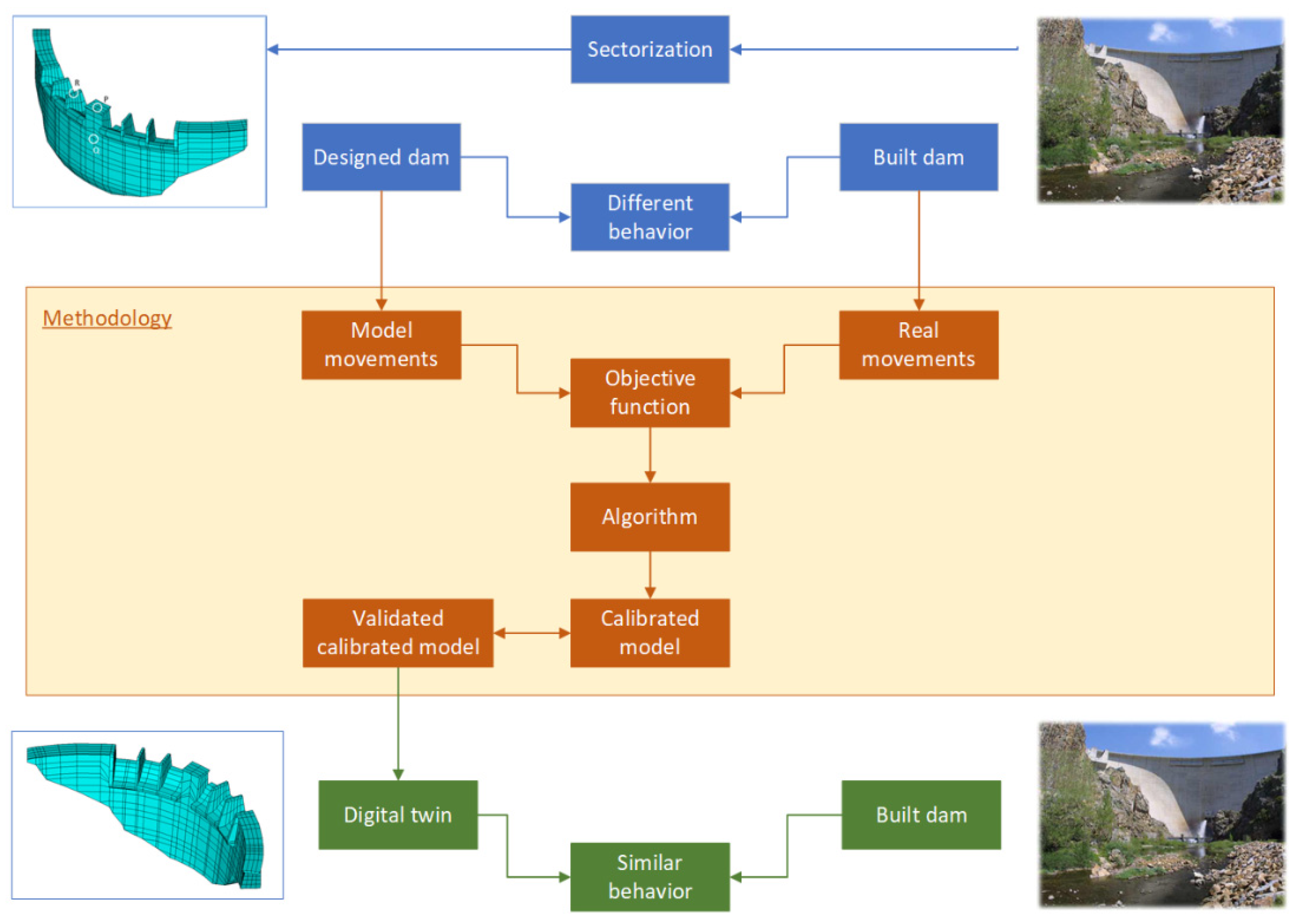
This process permitted the development of a sectorized digital twin of the real dam (Figure 1).
3. The Synthetic Arch Dam
As mentioned, the method used in this first phase of the research was applied to a synthetic dam represented by a numerical model. For practical purposes, the sectorization was limited to the foundation, where the variability of the stiffness parameters was usually higher than the variability in the dam concrete, as it depends on the geological configuration. Several sectorizations were considered, according to the most common situations encountered in dam foundations.
The use of a synthetic dam for research purposes has the advantage that the foundation is perfectly known and, therefore, its mechanical parameters, which will be determined by an optimization process, are known and accurate. In addition, the synthetic movements used for the optimization are accurate, because they lack the errors that are inherent in the measuring equipment, as well as accidental or human errors. Therefore, the accuracy of the calibration methodology can be determined in the absence of errors that are inherent due to the complexity of a real dam.
Further research is planned to verify the degree of accuracy that can be achieved in a real dam, with respect to which we will never be able to know the degree of adjustment in mechanical parameters, as they are unknown and difficult to estimate by testing. In this case, the validity of the calibration process will be determined by a comparison of predicted and measured movements.
The synthetic model contemplates a double curvature arch dam during the operation phase, with grouted joints. In this type of dam, it is common to have internal pendulums that measure the horizontal movements at various points inside the dam, coincident with the galleries through which the thread of each pendulum passes. These movements are normally complemented by the measurement of external movements at the crest and at the downstream face. Of all the movements that are usually measured in an arch dam, radial movements have been used to apply the proposed methodology, as radial movements are most representative of the behavior of the dam–foundation assembly and also the most reliable.
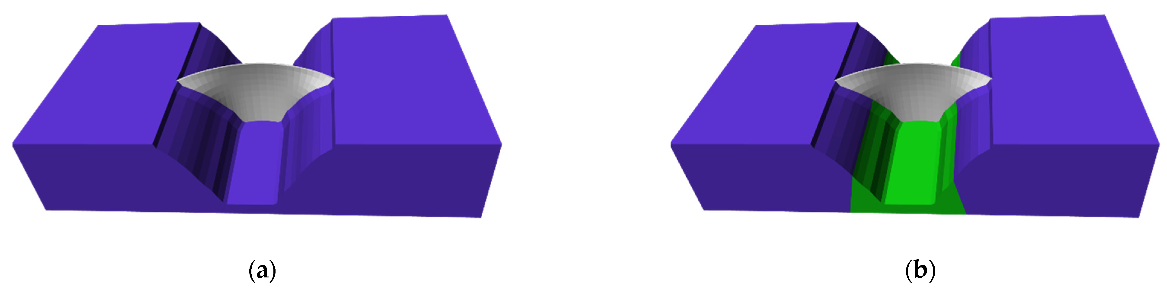
Two different foundation configurations were defined (Figure 2): (a) a homogeneous foundation, in which the two sectors of the entire foundation, the dam concrete and the foundation, have a similar mechanical behavior; and (b) a configuration with different stiffnesses in the dam abutments and the riverbed—i.e., the mechanical characteristics of the abutments are different from those of the soil in a riverbed. Therefore, there are three sectors in this case: the dam concrete, the riverbed, and the abutments. The two abutments have the same resistant parameters, but they are different from those of the riverbed sector.
The numerical models were developed in a Kratos environment, which is a framework for building multidisciplinary finite element programs. It provides several tools for the fast implementation of finite element applications: CFD, thermally coupled problems, particles, etc. [18], It was developed by the International Center for Numerical Methods in Engineering (CIMNE).
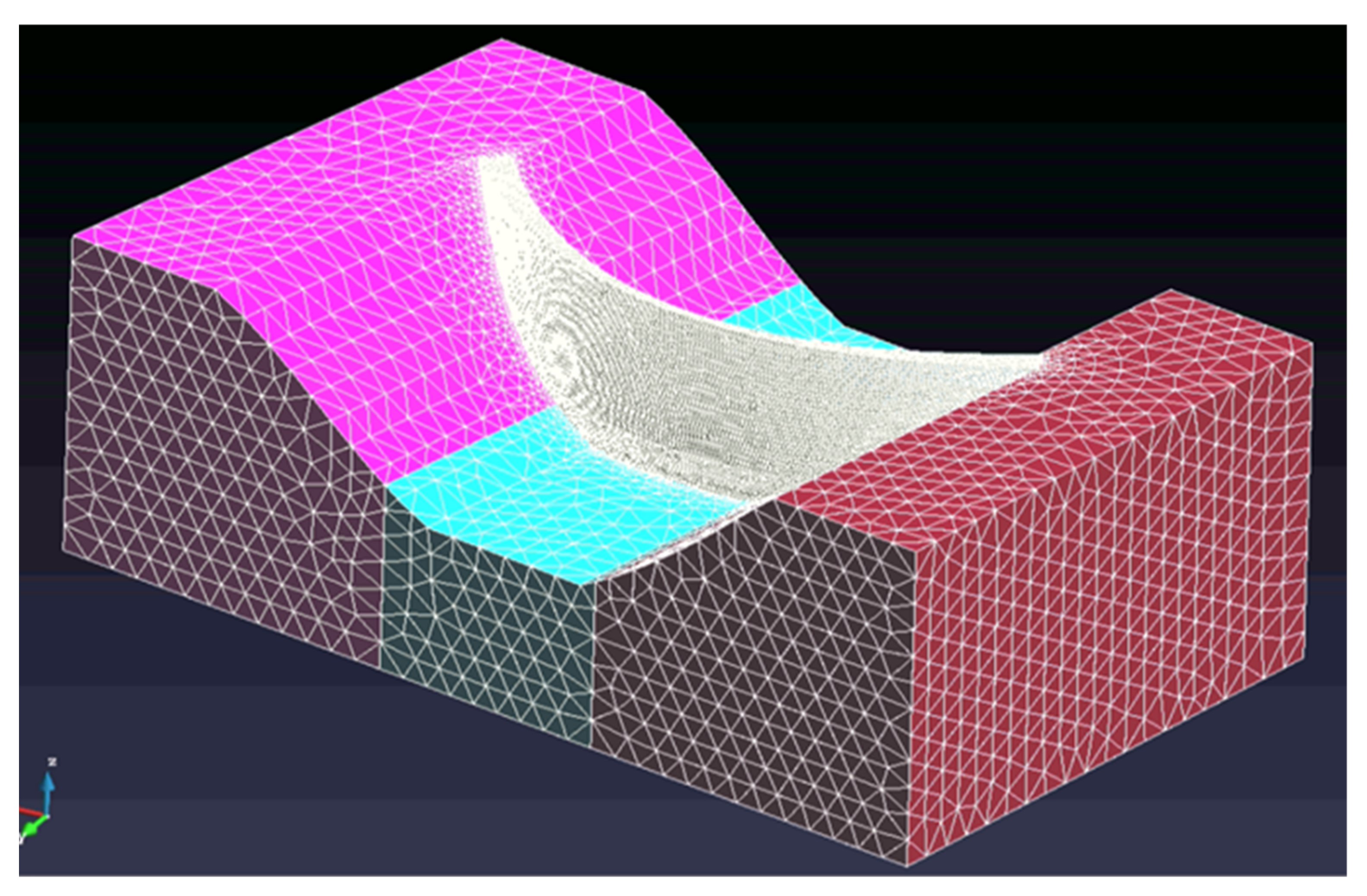
The finite element model of the dam had a total of 68,477 nodes and 363,756 elements (Figure 3). An unstructured mesh was used.
The calibration was performed in the most unfavorable load situation, with only self-weight, when the movements of the structure were minimal. With such small values of the radial movements, the relative errors might have reached very high values. Therefore, if the methodology was to provide good results for this demanding load situation, it was expected that the results would be at least as good in the rest of the situations, with larger movements. Although the modeled situation was purely theoretical and difficult to properly model for a real case, it was useful for the practical purposes of this research. Further research will focus on different loading conditions and applications in real cases.
4. Optimization Algorithm Based on the Gradient Descent: Methodology
4.1. The Algorithm
Many authors, including Ruder [19] and Haji et al. [20], have studied optimization algorithms based on gradient descent.
The procedure consists of forming a certain sequence of the following type:
where is the descent direction and is a scalar that is determined.
The descent direction is
and the algorithm is as follows (schematically represented in Figure 4):
- Stage 0: we set an initial value and a value .
- Stage k + 1:
We assumed for , at each step k, a value that would result exactly if the function were quadratic [21]:
The process ended when:
- and ;where ε and ε′ were two small prefixed values.
In our case, being f ≥ 0, due to the way it was defined, we could have changed the first condition to:
However, when the algorithm was applied to a real dam, the target values, which were used to define the function, contained errors inherent to the measurement, so it was very likely that this function would never reach zero value.
- If, after a predetermined number of steps () the above conditions were not met:
4.2. The Objective Function
For the creation of the objective function, the first task was to study the possible procedure to adjust the elastic properties of the materials that made up the structural dam–foundation assembly.
For this purpose, the objective function to be minimized was constructed. This function was defined on the basis that it depends on:
- the number of records of the monitorized instruments (first summation);
- the number of instruments to be considered (second summation);
- the number of movements, as this case has been studied with pendulum movements, measured in the horizontal plane (third summation).
- The final function to be minimized had the following form:
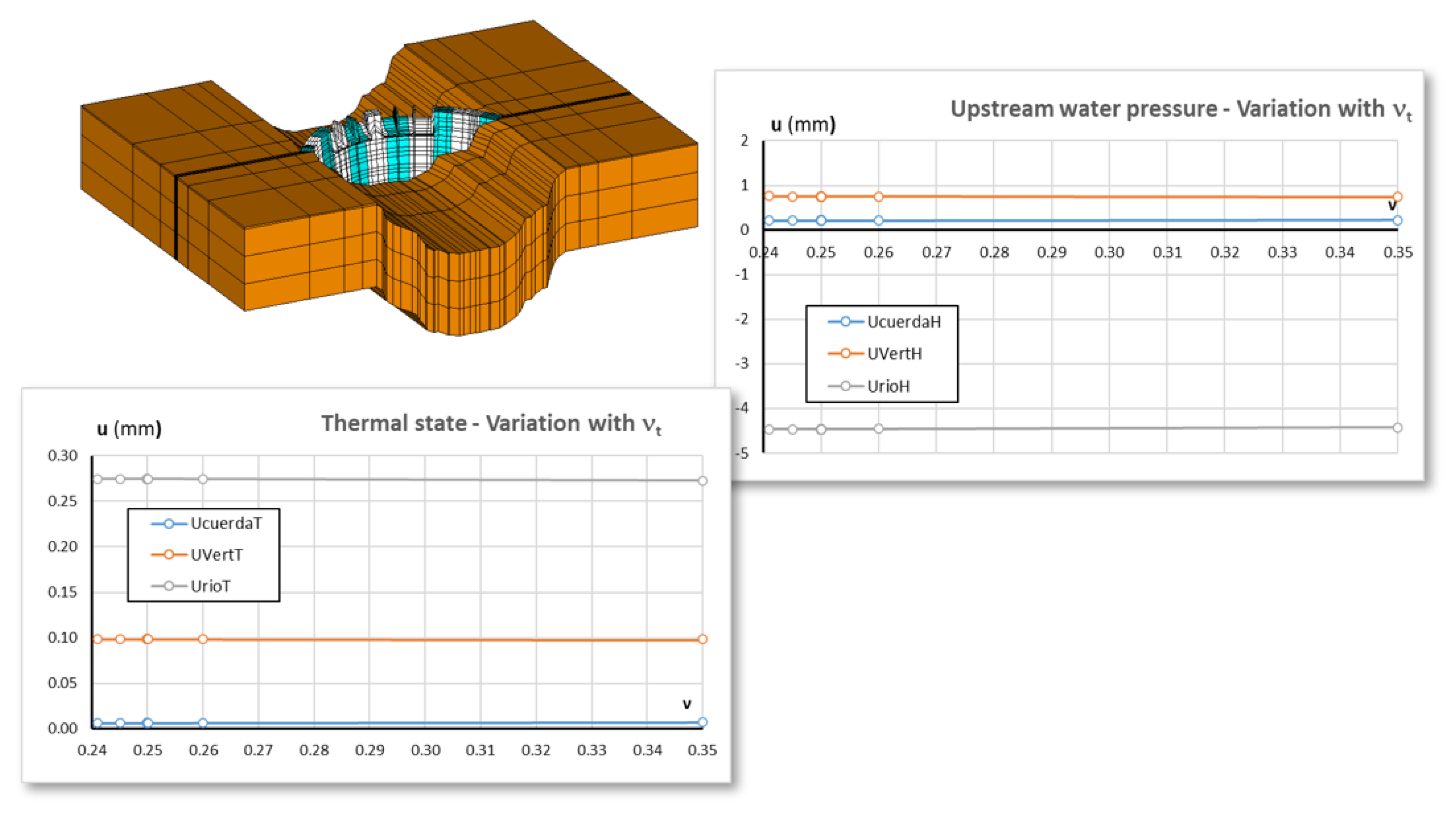
Once the function was defined, the sensitivity of the function to the variation of the Poisson ratio was studied. In the definition of the objective function, it was assumed that it depends exclusively on the values of the modulus of elasticity when it was obvious that, in elastic models, the materials also depended on the Poisson ratio .
This was done because practice indicates that this second parameter, in addition to being quite bounded, has little influence on the values of the motions if we move within these dimensions. To verify this, a numerical model, with fixed moduli of elasticity, was used to check the influence of the variation of the Poisson ratio. The conclusion obtained was that the influence of the variation of the Poisson ratio on the calculated movements was practically null as shown in Figure 5.
Other authors focused the optimization directly on the modulus of elasticity, disregarding the effect that the Poisson ratio may have [13,22]. The Poisson ratio used for the concrete was 0.20, and 0.25 for the foundation.
Having verified that the Poisson ratio had little influence, we proceeded to analyze the behavior of the function to be minimized in the proposed model. The performance was found to be not as expected, for two main reasons:
- The model used, without hydrostatic pressure, had very small movements close to zero, in which the error was triggered by the selected formulation.
- The moduli of elasticity of the soil and the dam differed by at least one order of magnitude, which made the weight of some modules more important than others, causing those less important modules not to be optimized.
For these reasons, the objective function to be minimized that was finally proposed was significantly different from the one previously stated, because it was necessary to make dimensionless both the elasticity modules and the relationship between the movements sought and the objective. Thus, the function finally used was:
where
was the motion at the point “i” obtained by the model;
was the objective motion at point “i”;
and, therefore, .
The objective function thus defined was the one that evaluated the error committed in each calculation. This function, by its own definition, tended to zero when the movements of the model were similar to those obtained by the monitoring system.
4.3. Improvements
The chosen gradient algorithm, despite being better than other algorithms studied for this particular application, converged slowly, due to the fact that the step value applied by means of the above formulation was very small. Evidently, this extreme became more evident as the number of unknown variables to be optimized and the number of control points increased.
Analyzing the performance of the algorithm, it can be seen that it was in the first steps that the algorithm advanced most rapidly toward the desired solution. A common tactic to accelerate convergence in this type of algorithm is to apply the algorithm in a certain number of steps, after which the point of the whole series with the best result of the imposed stopping conditions is analyzed and reapplied, taking this point as the starting point.
The algorithm, as usual, had several stopping conditions in order to avoid entering an infinite loop:
- The number of maximum steps was bounded. In the examples carried out, a maximum of 52 steps was used.
- The second condition was the number of cycles in which the algorithm stopped, and the results obtained were analyzed to determine the new starting point. In the examples carried out, eight cycles were used as a limit value.
These stopping criteria did not condition the solution obtained, because their amplitude allowed good approximations of the solution to be obtained with a calculation time that was not too long.
5. Optimization Algorithm Based on the Gradient Descent: Results and Discussion
The gradient method results depended greatly on the starting point. The same starting point was always used in the different iterations as more control movements were incorporated, in order to fairly compare the results of the algorithm.
As mentioned, the modulus of elasticity was chosen for the calibration process as the most relevant stiffness parameter of the materials.
5.1. Sectorization 1: Dam and Homogeneous Foundation
Two moduli of elasticity were considered: one for the dam and a different one for the foundation as a whole. The ranges considered for the elastic modulus of the concrete and the foundation were 16 GPa to 21 GPa and 2.9 GPa to 4.2 GPa, respectively. In this way, the domain of potential solutions in the plane (E1, E2) was defined.
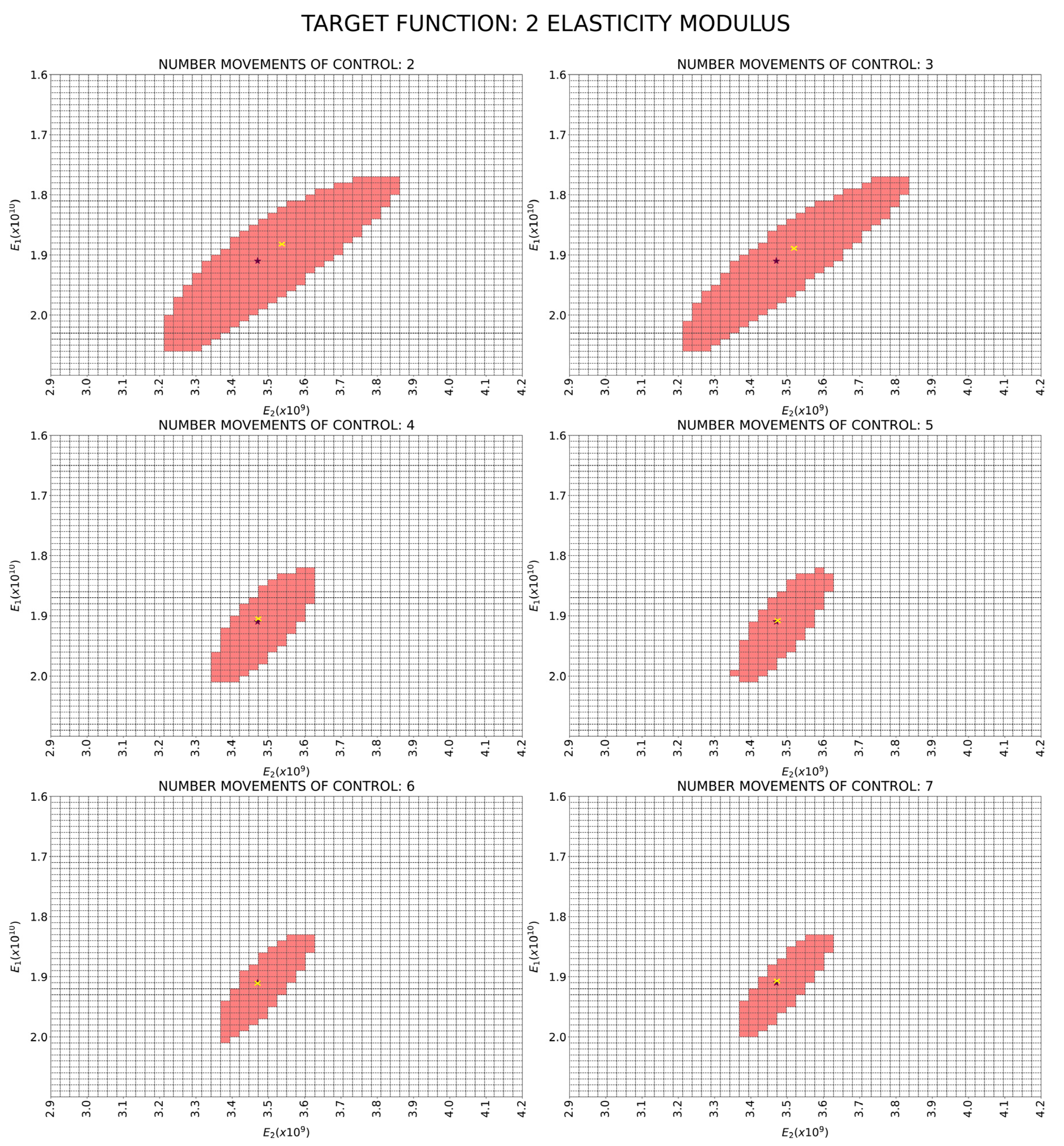
The number of radial movements available for calibration of a numerical model is variable in a real dam. For research purposes, from one to seven radial movements were considered in the optimization process. Therefore, the optimization method was run seven times, progressively including one to seven control movements. The objective function—that is, the mean error—as a difference between the real values of the dam movements and the calculated ones, was obtained for all points in the potential solution domain. In Figure 6, those points that meet the condition that the error is less than the maximum allowed value are represented in red. This red area is defined as the solution domain linked to a certain value of the maximum permitted error—in this case, one thousandth.
The point corresponding to the known moduli of elasticity that were used to compute the control movements in the synthetic dam was represented with a purple star, and the solution given by the optimization algorithm, the stopping point, was represented with a yellow cross.
When a single radial movement was used, the solution domain greatly expanded, most of it outside the potential solution domain considered. Therefore, we preferred to omit this case from the graphical representation, although the numerical result of the algorithm is included in Table 1.
The target values of the moduli of elasticity used to calculate the movements of the synthetic dam were 19.1 GPa for the dam concrete and 3.47 GPa for the foundation rock.
Regarding the error of the movements predicted by the calibrated model, the results were also quite accurate (Table 2). The mean square error (MSE) was considered [23,24] and the mean absolute error (MAE) was provided to compare between the metrics.
It can be observed that the relative error in the estimation of the elastic moduli of the concrete and the foundation material was less than 16%, even using a single control movement (Table 1). This error was quite low from a practical point of view, given the multiple uncertainties involved in the movement of an arch dam. Moreover, if we used only two control movements, the relative error dropped to under 2% for both elastic moduli, and to under 0.3% if we used four control movements in the optimization process.
The result was not always better if we increased the number of movements (from 5 onwards) for the calibration of the numerical model. Therefore, a low number of control movements was enough for a high precision calibration, and a high number of control movements did not guarantee a better result, despite the additional computational time.
From the analysis of Figure 6, two relevant conclusions can be drawn. The first is that the point that represents the known solution seemed to be close to the center of the solution domain in all the cases. The second is that the inclusion of additional control movements in the optimization process reduced the size of the solution domain, the red area in the figure, where the error was less than the maximum allowed value. This reduction was more relevant when the number of movements considered was low, and less clear for five control points or more. Therefore, for five control points or more, the result was extremely close to the exact solution, the result was not necessarily better for additional control points, and the solution domain size was not clearly reduced and remained quite similar.
The time required for optimization increased greatly with the addition of control points, so a balance was considered between the required precision and the computation time when deciding the number of control points to be considered.
5.2. Sectorization 2: Dam and Foundation Divided into Riverbed and Abutments
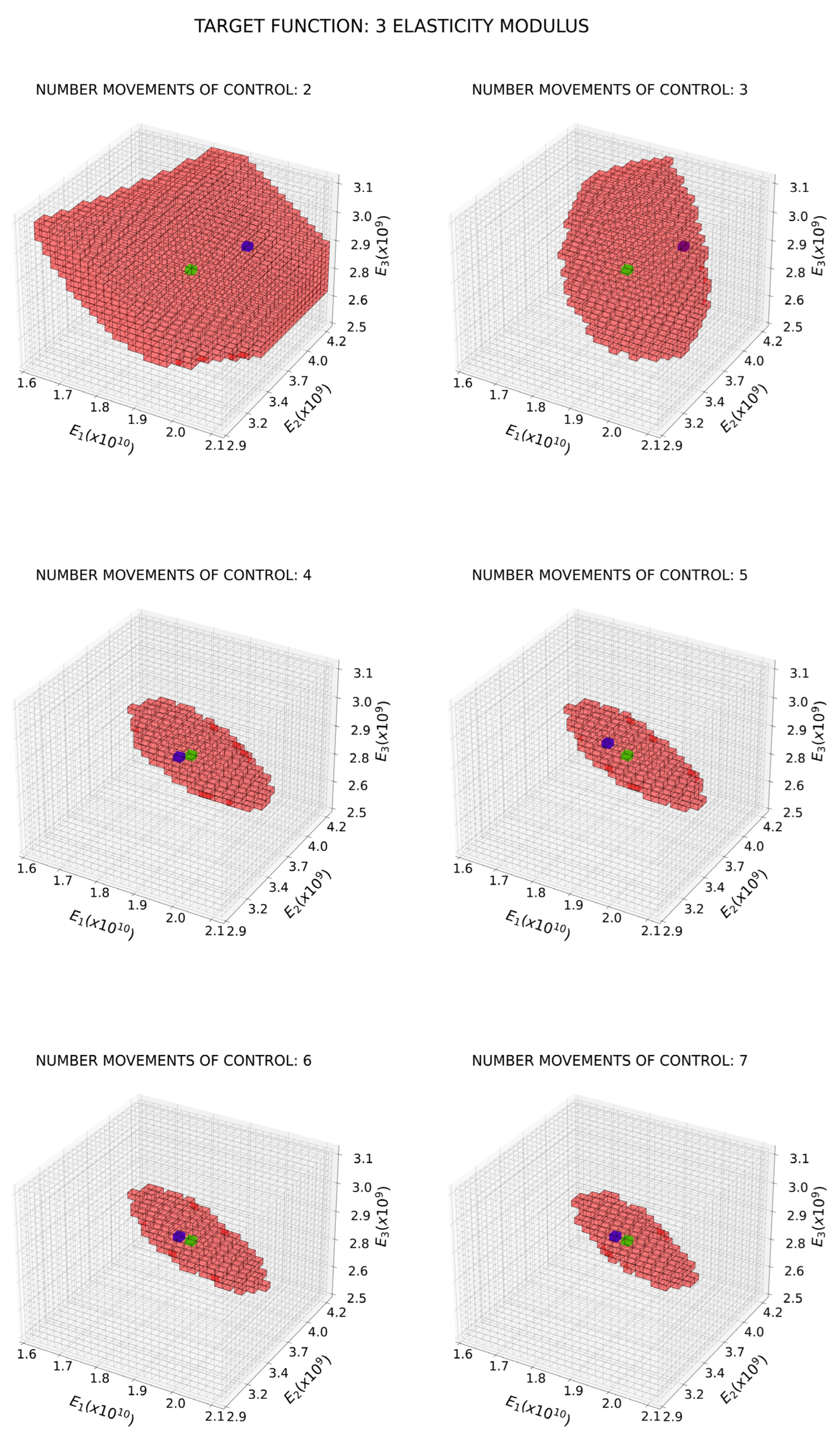
In this case, three moduli of elasticity were considered: one for the concrete dam (E1), another for the riverbed (E3), and a different one for both abutments (E2). Therefore, a 3D potential solution domain was defined, with ranges of 16 GPa to 21 GPa for E1, 2.9 GPa to 4.2 GPa for E2, and 2.5 GPa to 3.1 GPa for E3. As in sectorization 1, control movements between one and seven were progressively included. In addition, as in the case of sectorization 1, the relative error in the estimation of the elastic moduli was obtained for all the points (E1, E2, E3) of the potential solution space. The points where the error was lower than the maximum permitted error, that is, the solution domain, are marked in red in Figure 7. In this figure, the potential solution domain is represented by the volume of the whole parallelogram defined by the ranges, and the volume of the solution domain is represented in red (semi-translucid).
The point corresponding to the exact solution was represented with a green cube, and the stopping point of the algorithm, that is, the result of the optimization process, was represented with a blue cube. In addition, for this type of sectorization, for comparison purposes the same starting point was used in all the cases.
The target values of the moduli of elasticity, i.e., the values used for computing the movements on the synthetic dam, were 19.1 GPa for the dam concrete, 2.87 GPa for the riverbed material, and 3.47 GPa for the abutments rock. The results are shown in Table 3. Table 4 shows the errors (MSE and MAE) obtained in the control movements predicted by the calibrated model.
The results for sectorization 2, with three sectors of different moduli of elasticity, were consistent with those obtained for sectorization 1, with two sectors. Relative errors were lower than 15%, even for a single control movement, and lower than 1% for four control points; the results were not better for a higher number of control points. It should be noted that in scenarios with more than four movements, the algorithm stopped because the maximum number of steps was reached. If the number of steps were increased, better results might be obtained. Nevertheless, with the limitation of the current number of steps, the results were quite accurate.
The fit of the movements was not as accurate as for sectorization 1. However, the accuracy was still good.
6. The Centroid Method (CM)
A key property was observed in the first phase of the research: the exact solution was approximately centered in the solution domain, where the error was less than the maximum permitted value. This was observed in both the 2D and 3D potential solution spaces. The proposed centroid method is based on the hypothesis that the exact solution lies at the centroid of the solution space. Therefore, the centroid of the solution domain was proposed as the best estimate of the solution. Assuming this hypothesis, the solution could be determined with significantly fewer calculations than those needed when using the gradient descent method. Then, it was sufficient to perform the calculations required to obtain the centroid of the solution domain with the precision required for practical purposes.
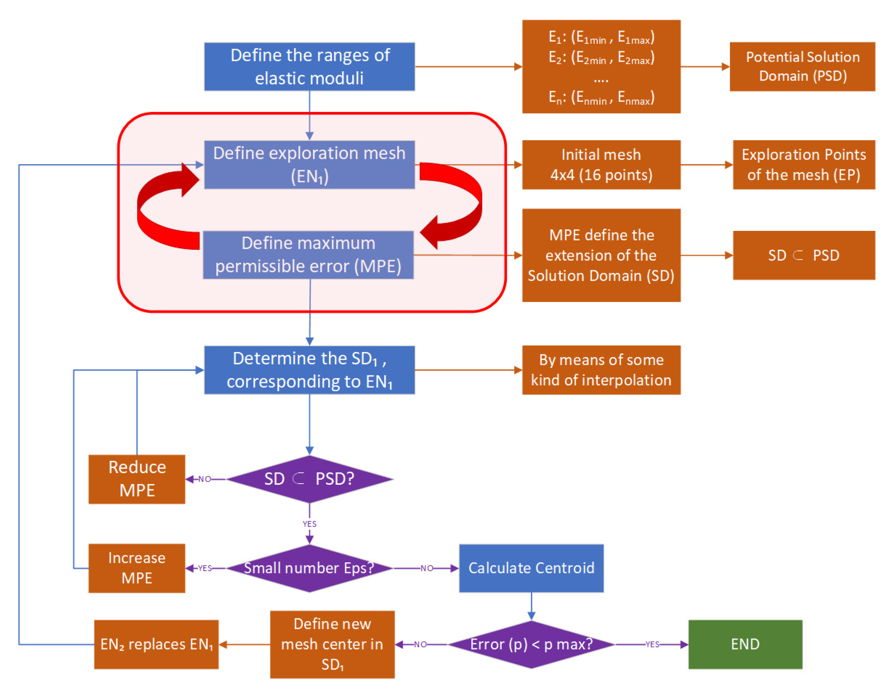
The process that was proposed to calibrate a digital twin of an arch dam, formulated in the most general way, followed a set of steps that can be automated (Figure 8):
- 1.
- Define the ranges of each of the elastic moduli (E) in which the solution will presumably be found. It is interesting to give amplitude to these ranges in order to be sure that the solution will be within the defined potential solution domain (PSD), but without more amplitude than necessary.
- 2.
- Define the initial exploration net (EN). This mesh must contain the smallest number of exploration points (EPs) that potentially might allow detecting the solution domain (SD). We proposed EN1 of 4 × 4 (16 EPs).
- 3.
- Calculate the movements at the control points of the dam corresponding to each EP of EN1 using the FEM model. Determine the prediction error at every EP.
- 4.
- Define the value of the maximum permitted error (MPE). The higher the MPE, the greater the extent of the solution domain. It is convenient for the SD to be large enough so that it is easily detectable with a small number of tries (exploration points, or EPs). However, it is necessary that the SD be completely contained in the PSD so that it is possible to determine the centroid. Therefore, the most appropriate value of the MPE must be established to ensure that the SD size meets the two above-mentioned requirements. It is easy to do so, taking into account the results obtained at the EPs of the EN1.
- 5.
- Determine the solution domain SD1, corresponding to EN1, by interpolation. It must be considered that:
- (a)
- It is convenient to automate the interpolation procedure.
- (b)
- A linear interpolation might work well; however, there is also the possibility of analyzing how the MPE varies in the horizontal and vertical directions and adopting the type of interpolation that best suits what is observed. This is a quick analysis, once automated, and might allow a reduction of the number of runs with the FEM model.
- (c)
- SD1 can be simply determined by joining with straight lines the points determined by interpolation. This could also be refined using curves.
- 6.
- Check that SD1 is completely contained in the PSD and that the size is sufficient for easy detection with a small number of EPs. If the MPE was properly chosen, the result will meet both conditions. However, a process must be considered if those conditions are not met.
- 6.1
- If SD1 exceeds the size of the PSD, the MPE value should be reduced. The process should return to step 5.
- 6.2
- If PSD1 is too small for easy definition with a small number of EPs, increase the MPE and return to step 5.
- 6.3
- If the size of PSD1 is judged to be adequate, proceed to determine its centroid. It will be considered as the best estimate of the solution.
- 7.
- Determine the mean error of the movement prediction at the control points (p).
- It should be noted that the error of the prediction of the elastic moduli of the different sectors cannot be determined in a real case, because the real value of the elastic moduli is unknown. However, determining this error is possible in the case of a synthetic dam and will be presented later.
- 7.1
- If the error (p) is acceptable, it is not necessary to refine the mesh, and the solution is accepted. For this purpose, a maximum acceptable error (pmax), which is different from the MPE, must be set.
- 7.2
- If the error (p) is excessive, the mesh must be refined, taking as the PSD a rectangle centered at the centroid determined in the previous step, containing the SD1, and leaving a margin to be fixed a priori (for example, as 20% of the maximum vertical dimension of the PSD1). In this new rectangle, the EN2 of 4 × 4 is defined and the process returns to Step 3.
The process is repeated until the error (p) is acceptable, lower than pmax.
7. Calibration of the Sectorized Digital Twin of the Synthetic Arch Dam Using the Centroid Method
The proposed new CM was used to calibrate several sectorized digital twins of the same synthetic arch dam described above, in order to compare the accuracy and number of calculations of both the gradient descent method, as a representative of a conventional optimization method, and the proposed centroid method.
7.1. Sectorization 1: Dam and Homogeneous Foundation
The specific way in which the CM was applied to this sectorization case was as follows:
- Initially, the PSD was defined. In this case, as a synthetic dam, the value of the target moduli of elasticity was known a priori. The ranks used are the same as those used in the gradient descent algorithm, 16 GPa to 21 GPa for the concrete (E1) and 2.9 GPa to 4.2 GPa for the foundation (E2)
- The maximum permitted error (MPE) was initially defined as 0.001, the same as was considered for the objective function used in the case of the gradient descent algorithm. This value was finally left unaltered.
- An exploration net (EN) of 36 points (6 × 6) was used to ensure that at least three EPs fell within the SD and that the SD was fully included in the PSD.
The case for two control points is represented, for clarity, in Figure 9. The mean prediction error was a surface in the PSD. That surface and the SD contained inside it were known from the calculations performed when using the gradient descent method. It was included in the graphs, as a reference, to better understand the process. However, it is important to note that they would not be known when calibrating the model of a real dam and they were not used when applying the CM. Only three points of the 6 × 6 exploration net, white with blue outline, were within the SD. These three points were the basis for applying the CM.
Next, a set of points approximating the SD boundary (red circles in Figure 9) was determined from the EPs belonging to the SD and adjacent EPs by parabolic interpolation. In order to reduce the noise when determining the centroid, points located in the same plane and on the same side of the SD boundary were eliminated, although it was an optional step with presumably low relevance for the final result.
- 4.
- Finally, the centroid of the SD was obtained from EPs that approximated the SD boundary. For that, a Delaunay triangulation was performed [25].
The results of applying the CM to calibrate the sectorized digital twin of the synthetic dam are summarized in Table 5, together with the results obtained by the gradient descent and grid search algorithms, for comparison.
It is clear that the calibration performed by the centroid method had a great accuracy, even better than that obtained by the gradient descent method, with a significantly lower computation time.
7.2. Sectorization 2: Dam and Foundation Divided into Riverbed and Abutments
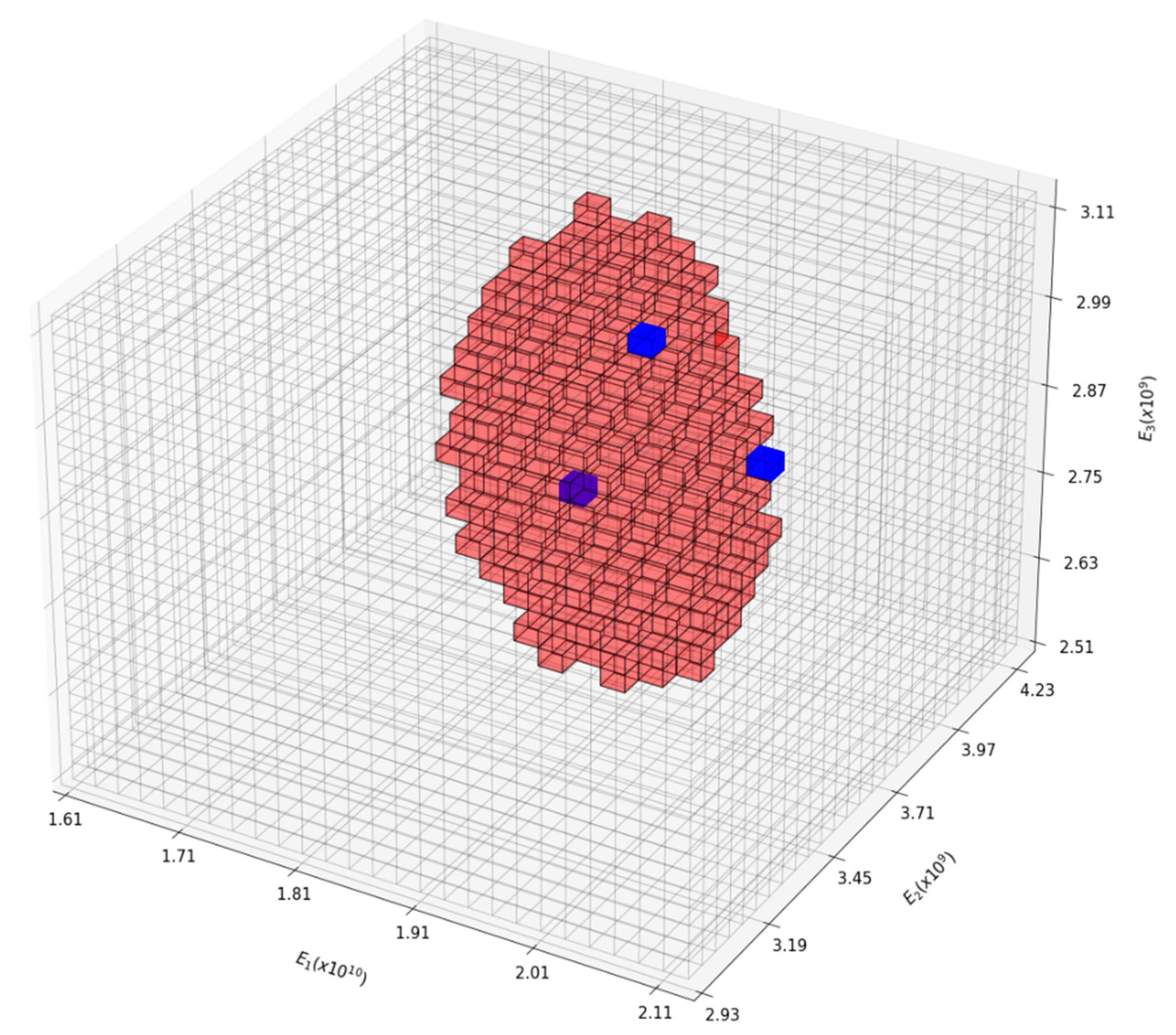
Following the same methodology described for the previous case, we studied the case of the foundation divided into two zones. The CM was applied to the case of three control movements. An exploration net EN 6 × 6 × 6 was considered, so that only three of the 216 EPs were within the SD (Figure 10).
The points or cubes that approximate the SD boundary were obtained from the three EPs inside the SD and the adjacent EPs by parabolic interpolation, following an analogous procedure as in the case of sectorization 1. Eighteen points (green cubes) were obtained this way. The lighter colored ones are at the front of the SD and the darker ones are at the back. The centroid of the SD was obtained from these eighteen points (black cube) (Figure 11).
The results are summarized in Table 6, together with the results obtained by the gradient descent and grid search algorithms, for comparison.
As in the case of sectorization 1, the centroid method provided accurate results that were more accurate than the gradient descent algorithm. In this case, the number of calculations needed by the CM was as low as 13.5% of those needed by the gradient descent method.
In this case, the result obtained by the CM was slightly less accurate than that obtained by the grid search method. However, the CM was still preferable, considering that the difference in precision was quite small (about 1.5% in the worst case), and eighty-one times fewer calculations were necessary.
7.3. Discussion about the Application of the Centroid Method and Future Research
The centroid method of optimization proved to be accurate and considerably cost-effective, in terms of computational time, compared with a conventional algorithm, the gradient descent method, for the purpose of calibrating the sectorized digital twin (SDT) of a synthetic arch dam based on a finite element model.
The results presented here are the first results of ongoing research, and future work will cover the use of different loading conditions, sectorizations, types of dams (including embankment dams), and the application to real cases in order to verify the degree of applicability of the method for the calibration of the SDT of dams and to quantify the efficiency in terms of computational time. In addition, the use of the CM for the calibration of numerical models corresponding to different types of structures, such as tunnels, bridges, and singular buildings, might be studied; there is no a priori reason for the CM not to work well in such cases.
The gradient descent algorithm requires a relatively large number of iterations for the algorithm to converge in the most demanding situations. The maximum number of calculations used depends on two variables: the number of parameters to be calibrated (Np) and the maximum number of steps (nmax). The number of calculations is defined by:
This algorithm heavily depends on the initial values chosen, so a good estimate of the initial moduli of elasticity of the problem is essential to limit the computational time. Therefore, the geotechnical study of the dam site, which is sometimes not as complete and rigorous as desired, is important for the application of this type of algorithm. It is different in the case of the centroid method, which only requires a rough estimate of the range for the target parameter. The use of the maximum permitted error makes it easy to fit the solution domain to the estimated range of the parameters that define the potential solution domain.
The extreme computational efficiency of the method opens up the possibility of treating cases that require multiple sectorization, with more than three areas, in order to take into account the variability of the material properties in the different zones of the foundation and the dam. In this way, the SDT might become closer to the complexity of a real dam by reducing the necessary simplification.
In the case of very heterogeneous foundations, a mean value of material properties of every identified sector might be used. In addition, a heterogeneous foundation might be modeled, in spite of adding an additional parameter for every sector.
The possibility of applying the CM, when very few or even one control point is available, is also interesting. In that case the accuracy of the grading descent method is lower and the number of cases that are necessary to solve might be greatly increased due to the huge extension of the solution domain. The CM is expected to work well and to be accurate in that case. It will be included in future work.
8. Summary and Conclusions
A new optimization algorithm, the centroid method, was proposed for the calibration of a sectorized digital twin (SDT) of an arch dam.
The time for the calibration of an SDT increases significantly as the numbers of parameters defining the material properties increase. Therefore, the development of efficient optimization algorithms is critical to the practical application of sectorization.
An improved optimization algorithm based on the gradient descent method was used to calibrate two SDTs of a synthetic dam, using a finite element model with two and three sectors. The calibration was performed on the hypothesis of one to seven available control points, where the radial movement was known. The modulus of elasticity was used as the target variable for optimization.
The mean relative error in the estimation of the elastic modulus of the different sectors was always less than 16%, even when only one control point was available, and less than 1.6% for more than three control points.
We observed that the exact solution, which was the target value of optimization, was approximately at the centroid of the solution domain, defined as the region of the (E1, E2) or (E1, E2, E3) space, depending on the sectorization case, where the prediction error was lower than a previously specified maximum permitted error. This clearly occurred in all of the considered cases.
Therefore, the hypothesis that the best estimate of the solution is at the centroid of the solution domain was the base for a new optimization algorithm, the centroid method. It was formulated in detail for practical use.
Two of the cases that were calibrated using the gradient descent method were also calibrated for comparison by means of the new centroid method, corresponding to the two types of sectorization that were considered.
The solution obtained by using the centroid method was even more accurate in both cases and, more importantly, the number of models solved along the optimization process was considerably lower: i.e., 8% of the solved models were needed by the gradient descent method for the sectorization case with two sectors, and 13.5% were needed for the sectorization case with three sectors.
The great efficiency and low time consumption of the centroid method opens up the practical possibility of calibrating more complex sectorized digital twins that better approximate the behavior of a real dam and foundation.
In addition, an accurate and low time-consuming calibration is expected for cases when only one control point is available.
The preliminary results of the ongoing research for models with more than three sectors also show good accuracy and low computational time, despite the higher complexity of the models.
More research is needed to consider several load conditions, numbers of sectors, the typology of a dam, and the application of the model to real cases and to different types of structures.
Author Contributions
Conceptualization, E.R.C.L., M.Á.T. and E.S.C.; methodology, E.R.C.L., M.Á.T. and E.S.C.; software, E.R.C.L.; formal analysis, E.R.C.L., M.Á.T. and E.S.C.; investigation, E.R.C.L.; data curation, E.R.C.L.; writing—original draft preparation, E.R.C.L.; writing—review and editing, M.Á.T. and E.S.C.; visualization, E.R.C.L.; supervision, M.Á.T. and E.S.C. All authors have read and agreed to the published version of the manuscript.
Funding
This research was funded by the NUMA project (grant number RTC-2016-4859-5), which was funded by the Ministry of Economy, Industry and Competitiveness of Spain.
Data Availability Statement
The data are not available, for confidential reasons.
Acknowledgments
The authors would like to acknowledge the collaboration of Fernando Salazar and David Vicente from the International Center for Numerical Methods in Engineering (CIMNE).
Conflicts of Interest
The authors declare no conflict of interest.
Nomenclature
| CIMNE | International Center of Numerical Methods in Engineering |
| CFD | Computational fluids dynamics |
| CM | Centroid method |
| EN | Exploration net |
| EP | Exploration points |
| MPE | Maximun permitted error |
| PSD | Potential solution domain |
| SD | Solution domain |
| SDT | Sectorized digital twin |
| A symmetric positive definite matrix that can be constant or variable with the step | |
| Modulus of elasticity of the material “i” | |
| Initial modulus of elasticity of the material “i” | |
| Enmin | Minimum value of the modulus of elasticity “n” |
| Enmax | Maximum value of the modulus of elasticity “n” |
| Generic function | |
| Number of instruments to be considered. | |
| Number of movements in the horizontal plane. | |
| nmax | the maximum number of steps in the gradient descent algorithm |
| Np | number of parameters to be calibrated in the gradient descent algorithm |
| pmax | Maximum acceptable relative error |
| R | Number of records of the monitorized instruments. |
| The values measured by the instrument j, in the register R. | |
| The movements obtained with the model in the instrument j, in the register R, dependent on the values of the moduli of elasticity. | |
| Motion at the point “i” obtained by the model | |
| Objective motion at point “i”. | |
| A scalar that determines the advance in the direction of the gradient of the function at a point | |
| The n principal corner minors containing the first row and first column element | |
| ε and ε’ | Two small values that determine the errors allowed in the algorithm |
| (also | The values of the gradient vector at the point |
| The Hessian matrix at the point | |
| Poisson ratio |
References
- Vilardell, J.; Aguado, A.; Agullo, L.; Gettu, R. Estimation of the modulus of elasticity for dam concrete. Cem. Concr. Res. 1998, 28, 93–101. [Google Scholar] [CrossRef]
- Zhou, W.; Li, S.; Ma, G.; Chang, X.; Ma, X.; Zhang, C. Parameters inversion of high central core rockfill dams based on a novel genetic algorithm. Sci. China Technol. Sci. 2016, 59, 783–794. [Google Scholar] [CrossRef]
- Wu, Z.R.; Gu, Y.C.; Gu, C.S.; Guo, H.Q.; Su, H.Z. Establishing time-dependent model of deformation modulus caused by bedrock excavation rebound by inverse analysis method. Sci. China Ser. E 2008, 51, 1–7. [Google Scholar] [CrossRef]
- Ardito, R.; Maier, G.; Massalongo, G. Diagnostic analysis of concrete dams based on seasonal hydrostatic loading. Eng. Struct. 2008, 30, 3176–3185. [Google Scholar] [CrossRef]
- Su, H.Z.; Wen, Z.P.; Zhang, S.; Tian, S.G. Method for choosing the optimal resource in back-analysis for multiple material parameters of a dam and its foundation. J. Comput. Civ. Eng. 2015, 30, 04015060. [Google Scholar] [CrossRef]
- Labibzadeh, M.; Khajehdezfuly, A.; Khayat, M.; Arab, Y. Elastic strength diagnosis of the dez concrete arch dam using thermal inverse analysis. J. Perform. Constr. Facil. 2015, 29, 04014167. [Google Scholar] [CrossRef]
- Su, H.Z.; Zhang, S.; Wen, Z.P.; Li, H. Prototype monitoring data-based analysis of time varying material parameters of dams and their foundation with structural reinforcement. Eng. Comput.-Ger. 2017, 33, 1027–1043. [Google Scholar] [CrossRef]
- Nguyen-Tuan, L.; Könke, C.; Lahmer, T. Damage identification using inverse analysis for 3D coupled thermo-hydro-mechanical problems. Comput. Struct. 2018, 196, 146–156. [Google Scholar] [CrossRef]
- Kang, F.; Liu, X.; Junjie, L.; Hongjun, L. Multi-parameter inverse analysis of concrete dams using kernel extreme learning machines-based response surface model. Eng. Struct. 2022, 256, 113999. [Google Scholar] [CrossRef]
- De Sortis, A.; Paoliani, P. Statistical analysis and structural identification in concrete dam monitoring. Eng. Struct. 2007, 29, 110–120. [Google Scholar] [CrossRef]
- Lifu, Y.; Huaizhi, S.; Zhiping, W. Improved PLS and PSO methods-based back analysis for elastic modulus of dam. Adv. Eng. Softw. 2019, 131, 205–216. [Google Scholar] [CrossRef]
- Chaoning, L.; Tongchun, L.; Siyu, C.; Chuan, L.; Xiaoqing, L.; Lingang, G.; Taozhen, S. Structural identification in long-term deformation characteristic of dam foundation using meta-heuristic optimization techniques. Adv. Eng. Softw. 2020, 148, 12870. [Google Scholar] [CrossRef]
- Fedele, R.; Maier, G.; Miller, B. Health assessment of concrete dams by overall inverse analyses and neural networks. Int. J. Fract. 2006, 137, 151–172. [Google Scholar] [CrossRef]
- Fedele, R.; Maier, G.; Miller, B. Identification of elastic stiffness and local stresses in concrete dams by in situ tests and neural networks. Struct. Infrastruct. Eng. 2005, 1, 165–180. [Google Scholar] [CrossRef]
- Yu, Y.; Zhang, B.; Yuan, H. An intelligent displacement back-analysis method for earth-rockfill dams. Comput. Geotech. 2007, 34, 423–434. [Google Scholar] [CrossRef]
- Mata, J. Interpretation of concrete dam behaviour with artificial neural network and multiple linear regression models. Eng. Struct. 2011, 33, 903–910. [Google Scholar] [CrossRef]
- Liu, X.; Kang, F.; Ma, C.; Li, H. Concrete arch dam behavior prediction using kernel-extreme learning machines considering thermal effect. J. Civ. Struct. Health Monit. 2021, 11, 283–299. [Google Scholar] [CrossRef]
- Kratos, Multiphysics Open Source FEM Code. Available online: https://www.cimne.com/kratos (accessed on 1 August 2022).
- Ruder, S. An Overview of Gradient Descent Optimization Algorithms. 2016. Available online: https://arxiv.org/abs/1609.04747 (accessed on 7 September 2022).
- Haji, S.H.; Abdulazeez, A.M. Comparison of optimization techniques based on gradient descent algorithm: A review. PalArch’s J. Archaeol. Egypt/Egyptol. 2021, 18, 2715–2743. Available online: https://www.archives.palarch.nl/index.php/jae/article/view/6705 (accessed on 7 September 2022).
- Barzilai, J.; Borwein, J.M. Two-point step size gradient methods. IMA J. Numer. Anal. 1988, 8, 141–148. [Google Scholar] [CrossRef]
- Wang, W.; Kuang, Y.; Li, S.; Ni, X. Back analysis of dam parameter under seismic action. Procedia Eng. 2012, 28, 429–433. [Google Scholar] [CrossRef]
- Theobald, C.M. Generalizations of mean square error applied to ridge regression. J. R. Stat. Soc. Ser. B 1974, 36, 103–106. [Google Scholar] [CrossRef]
- Hodson, T.O. Root-mean-square error (RMSE) or mean absolute error (MAE): When to use them or not. Geosci. Model Dev. 2022, 15, 5481–5487. [Google Scholar] [CrossRef]
- Chen, L.; Xu, J.C. Optimal Delaunay triangulations. J. Comput. Math. 2004, 22, 299–308. Available online: https://www.jstor.org/stable/43693155 (accessed on 7 September 2022).
Figure 1.
Process to develop a sectorized digital twin.

Figure 2.
Sectorization of the model: (a) two moduli of elasticity: grey for the dam (E1) and blue for the homogeneous foundation (E2); (b) three moduli of elasticity: grey for the dam (E1), blue for both abutments (E2), and green for the riverbed (E3).
Figure 2.
Sectorization of the model: (a) two moduli of elasticity: grey for the dam (E1) and blue for the homogeneous foundation (E2); (b) three moduli of elasticity: grey for the dam (E1), blue for both abutments (E2), and green for the riverbed (E3).

Figure 3.
Synthetic dam meshing.

Figure 4.
Gradient algorithm performance.

Figure 5.
Study of the sensitivity of dam movement to changes in the Poisson ratio.

Figure 6.
Calibration of the dam with homogeneous foundation with different numbers of control movements. (E1 modulus of elasticity of concrete (Pa); E2 modulus of elasticity of the foundation (Pa)).
Figure 6.
Calibration of the dam with homogeneous foundation with different numbers of control movements. (E1 modulus of elasticity of concrete (Pa); E2 modulus of elasticity of the foundation (Pa)).

Figure 7.
Calibration of the dam and the foundation, divided into riverbed and abutments, with a different number of control movements. (E1 modulus of elasticity of concrete (Pa), E2 modulus of elasticity for the riverbed (Pa), and E3 modulus of elasticity for the abutments (Pa)). The green cube represents the volume in which the exact solution is placed. The blue cube is the volume where the result of the optimization process is placed.

Figure 8.
The centroid method.

Figure 9.
Sectorization 1 (2D). Number of control points: 2. The white dots pertain to the 6 × 6 exploration net (EN). The blue area is the solution domain obtained by applying a grid search algorithm. The red dots are the approximate points, obtained by interpolation, that define the boundary of the SD. The green dot is the calculated centroid. E1 and E2 are the moduli of elasticity of the concrete and the foundation, respectively (Pa).

Figure 10.
Sectorization 2 (3D). Number of control points: 3. E1, E2, and E3 are the moduli of elasticity of concrete and foundation, riverbed, and abutments, respectively (Pa). The SD is a 3D volume obtained when applying a grid search algorithm (red in the figure). Blue cubes correspond to the 6 × 6 × 6 exploration net (EN) and are inside the SD.

Figure 11.
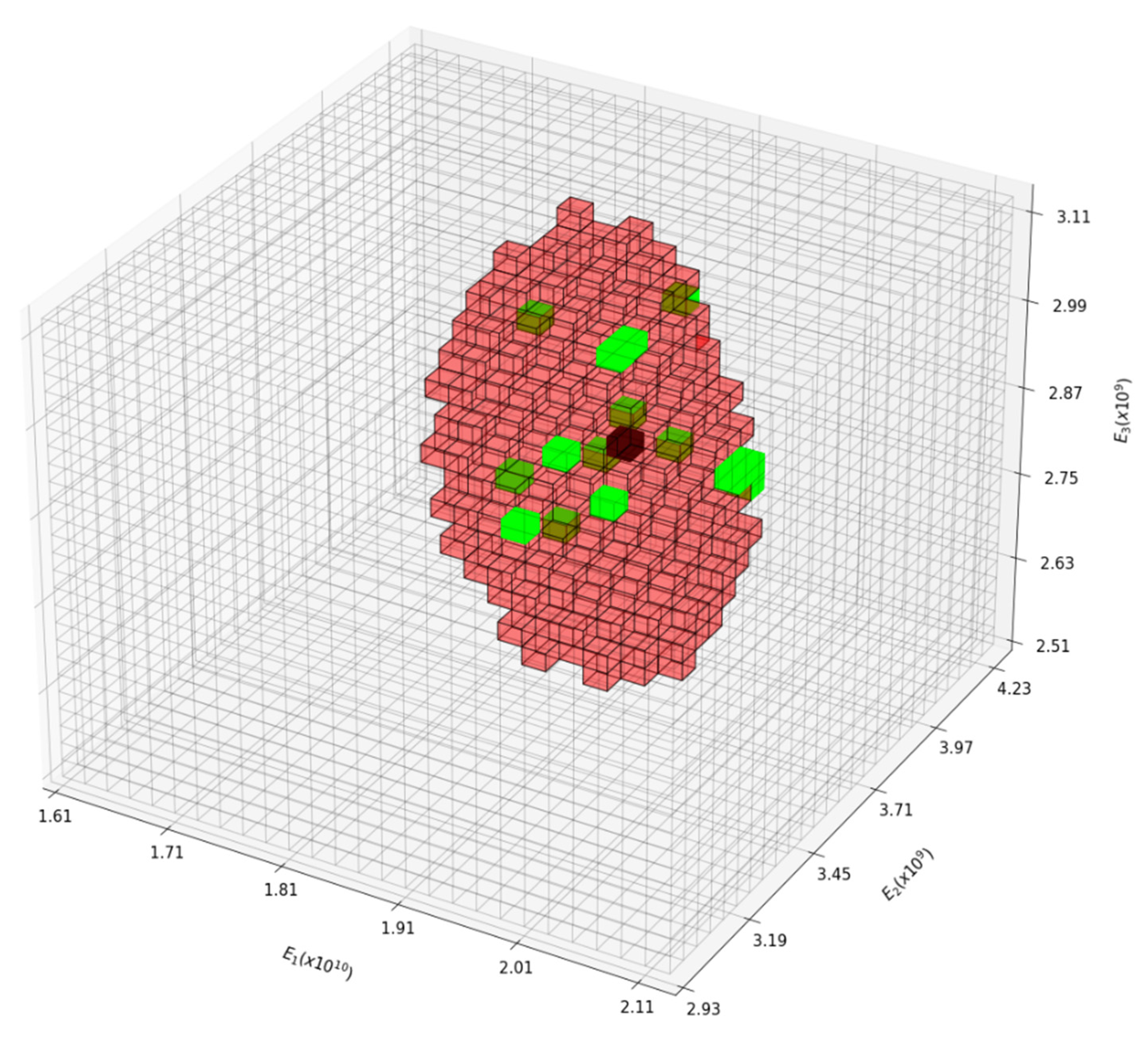
Sectorization 2 (3D). Number of control points: 3. E1, E2, and E3 are the moduli of elasticity of concrete and foundation, riverbed, and abutments, respectively (Pa). The SD is a 3D volume obtained when applying a grid search algorithm (red in the figure). Green cubes are the 18 points that approximate the SD boundary; the lighter colored ones are on the front face of the SD and the darker ones at the back face. The black cube is the centroid.
Figure 11.
Sectorization 2 (3D). Number of control points: 3. E1, E2, and E3 are the moduli of elasticity of concrete and foundation, riverbed, and abutments, respectively (Pa). The SD is a 3D volume obtained when applying a grid search algorithm (red in the figure). Green cubes are the 18 points that approximate the SD boundary; the lighter colored ones are on the front face of the SD and the darker ones at the back face. The black cube is the centroid.


Table 1.
Calibrated elasticity moduli for sectorization 1: dam and homogeneous foundation.
| Calculated Moduli of Elasticity (Pa) | Calculation Error 1 | |||
|---|---|---|---|---|
| Nº of Movements | E1 (Dam) | E2 (Foundation) | E1 (Dam) | E2 (Foundation) |
| 1 | 1.794 × 10¹⁰ | 3.998 × 10⁹ | −6.07% | 15.22% |
| 2 | 1.882 × 10¹⁰ | 3.537 × 10⁹ | −1.47% | 1.93% |
| 3 | 1.889 × 10¹⁰ | 3.519 × 10⁹ | −1.10% | 1.41% |
| 4 | 1.905 × 10¹⁰ | 3.472 × 10⁹ | −0.26% | 0.06% |
| 5 | 1.908 × 10¹⁰ | 3.474 × 10⁹ | −0.10% | 0.12% |
| 6 | 1.911 × 10¹⁰ | 3.470 × 10⁹ | 0.05% | 0.00% |
| 7 | 1.907 × 10¹⁰ | 3.472 × 10⁹ | −0.16% | 0.06% |
1 This error is the relative error made in the estimation of the modulus of elasticity. The relative error is calculated as the searched value minus the calculated value and divided by the searched value.
Table 2.
Error of movement estimation for sectorization 1: dam and homogeneous foundation.
| Movements | MSE (Pa2) | MAE (Pa) |
|---|---|---|
| 1 | 1.204 × 10⁻¹³ | 3.470 × 10⁻⁷ |
| 2 | 1.529 × 10⁻¹¹ | 3.342 × 10⁻⁶ |
| 3 | 4.173 × 10⁻¹³ | 5.062 × 10⁻⁷ |
| 4 | 8.470 × 10⁻¹⁴ | 2.255 × 10⁻⁷ |
| 5 | 4.909 × 10⁻¹⁴ | 1.676 × 10⁻⁷ |
| 6 | 1.066 × 10⁻¹⁴ | 8.278 × 10⁻⁸ |
| 7 | 2.341 × 10⁻¹⁴ | 1.246 × 10⁻⁷ |
Table 3.
Calibrated elasticity moduli for sectorization 2: dam and foundation divided into riverbed and abutments.
Table 3.
Calibrated elasticity moduli for sectorization 2: dam and foundation divided into riverbed and abutments.
| Calculated Moduli of Elasticity (Pa) | Calculation Error 1 | |||||
|---|---|---|---|---|---|---|
| Nº of Movements | E1 (Dam) | E2 (Riverbed) | E3 (Abutments) | E1 | E2 | E3 |
| 1 | 1.864 × 10¹⁰ | 3.964 × 10⁹ | 3.083 × 10⁹ | −2.41% | 14.24% | 7.42% |
| 2 | 1.969 × 10¹⁰ | 3.892 × 10⁹ | 2.860 × 10⁹ | 3.09% | 12.16% | −0.35% |
| 3 | 1.860 × 10¹⁰ | 3.631 × 10⁹ | 2.970 × 10⁹ | −2.62% | 4.64% | 3.48% |
| 4 | 1.894 × 10¹⁰ | 3.459 × 10⁹ | 2.881 × 10⁹ | −0.84% | −0.32% | 0.38% |
| 5 | 1.880 × 10¹⁰ | 3.471 × 10⁹ | 2.899 × 10⁹ | −1.57% | 0.03% | 1.01% |
| 6 | 1.881 × 10¹⁰ | 3.471 × 10⁹ | 2.899 × 10⁹ | −1.52% | 0.03% | 1.01% |
| 7 | 1.883 × 10¹⁰ | 3.459 × 10⁹ | 2.889 × 10⁹ | −1.41% | −0.32% | 0.66% |
1 As in the case of sectorization 1, this error is the relative error made in the estimation of the modulus of elasticity. The relative error is calculated as the target value minus the calculated value and divided by the target value.
Table 4.
Error of movement estimation for sectorization 2: dam and foundation divided into riverbed and abutments.
Table 4.
Error of movement estimation for sectorization 2: dam and foundation divided into riverbed and abutments.
| Nº of Movements | MSE (Pa2) | MAE (Pa) |
|---|---|---|
| 1 | 1.336 × 10⁻⁹ | 3.656 × 10⁻⁵ |
| 2 | 6.819 × 10⁻¹⁰ | 1.911 × 10⁻⁵ |
| 3 | 1.796 × 10⁻⁹ | 3.406 × 10⁻⁵ |
| 4 | 2.863 × 10⁻⁹ | 4.655 × 10⁻⁵ |
| 5 | 3.641 × 10⁻⁹ | 5.339 × 10⁻⁵ |
| 6 | 8.780 × 10⁻¹⁰ | 2.250 × 10⁻⁵ |
| 7 | 1.162 × 10⁻⁹ | 2.817 × 10⁻⁵ |
Table 5.
Comparison of the results of the different methodologies employed. Dam and homogeneous foundation.
Table 5.
Comparison of the results of the different methodologies employed. Dam and homogeneous foundation.
| Modulus of Elasticity (Pa) | Relative Error 1 | ||||
|---|---|---|---|---|---|
| Optimization Method | Nº of Calculus | E1 (dam) | E2 (foundation) | Error E1 | Error E2 |
| Target values | 1.910 × 10¹⁰ | 3.470 × 10⁹ | |||
| Gradient descent | 456 | 1.882 × 10¹⁰ | 3.537 × 10⁹ | −1.47% | 1.93% |
| Grid search | 2601 | 1.909 × 10¹⁰ | 3.506 × 10⁹ | −0.052% | 1.037% |
| Centroid | 37 | 1.911 × 10¹⁰ | 3.486 × 10⁹ | 0.054% | 0.471% |
1 Relative error made in the estimation of the modulus of elasticity, taking as a reference the target value.
Table 6.
Comparison of the results of the different methodologies employed. Dam and foundation divided into riverbed and abutments.
Table 6.
Comparison of the results of the different methodologies employed. Dam and foundation divided into riverbed and abutments.
| Modulus of Elasticity (Pa) | Relative Error 1 | ||||||
|---|---|---|---|---|---|---|---|
| Optimization Method | Nº of Calculus | E1 (Dam) | E2 (Abutments) | E3 (Riverbed) | Error E1 | Error E2 | Error E3 |
| Target values | 1.910 × 10¹⁰ | 3.470 × 10⁹ | |||||
| Gradient descent | 1604 | 1.860 × 10¹⁰ | 3.631 × 10⁹ | 2.970 × 10⁹ | −2.606% | 4.626% | 3.496% |
| Grid search | 17,576 | 1.910 × 10¹⁰ | 3.551 × 10⁹ | 2.895 × 10⁹ | 0.005% | 2.331% | 0.868% |
| Centroid | 217 | 1.929 × 10¹⁰ | 3.605 × 10⁹ | 2.897 × 10⁹ | 1.011% | 3.903% | 0.932% |
1 Relative error made in the estimation of the modulus of elasticity, taking as a reference the target value.
Publisher’s Note: MDPI stays neutral with regard to jurisdictional claims in published maps and institutional affiliations. |
© 2022 by the authors. Licensee MDPI, Basel, Switzerland. This article is an open access article distributed under the terms and conditions of the Creative Commons Attribution (CC BY) license (https://creativecommons.org/licenses/by/4.0/).
Share and Cite
MDPI and ACS Style
Conde López, E.R.; Toledo, M.Á.; Salete Casino, E. The Centroid Method for the Calibration of a Sectorized Digital Twin of an Arch Dam. Water 2022, 14, 3051. https://doi.org/10.3390/w14193051
AMA Style
Conde López ER, Toledo MÁ, Salete Casino E. The Centroid Method for the Calibration of a Sectorized Digital Twin of an Arch Dam. Water. 2022; 14(19):3051. https://doi.org/10.3390/w14193051
Chicago/Turabian StyleConde López, Eduardo R., Miguel Á. Toledo, and Eduardo Salete Casino. 2022. "The Centroid Method for the Calibration of a Sectorized Digital Twin of an Arch Dam" Water 14, no. 19: 3051. https://doi.org/10.3390/w14193051
Note that from the first issue of 2016, this journal uses article numbers instead of page numbers. See further details here.