Soil Salinity Patterns in an Olive Grove Irrigated with Reclaimed Table Olive Processing Wastewater

Abstract

The agricultural use of saline table olive processing wastewater enables the implementation of closed water cycles in this socioeconomically important industry for rural southern Spain and relieves environmental, economic, and legal burdens. To allow growers to evaluate and guarantee adequate long-term soil and plant conditions when irrigating with such regenerated wastewaters, efficient soil monitoring strategies are needed. Field-scale monitoring with electromagnetic induction sensing, after one (2013) and five years (2017) of irrigation with regenerated wastewater with average electrical conductivity (EC) near 6 dS m⁻¹ in an olive orchard in southern Spain, showed accumulation of highly conductive material in the subsoil in relation to local topography and soil characteristics. Laboratory analysis of the soil water revealed strongly varying patterns of EC during the growing season and across the olive grove, which were attributed to dilution and concentration effects due to rainfall and evaporation, respectively. Visual inspection and leaf analyses revealed no negative effects on the olive trees. Apparent electrical conductivity (ECa), measured in between the tree rows in 2013, showed a linear relationship with surface soil EC_1:5 under the drippers and allowed identification of areas with high ECa in the low elevation zones of the farm, due to the presence of shallow perched saline water tables. A second ECa measurement in 2017 showed similar spatial ECa patterns and was used to estimate the distribution of soil EC across the soil profile using inversion software, although no unique field-wide relationships with soil properties could be inferred, possibly as a consequence of spatially variable soil clay and water contents, due to the influence of the topography. Despite the implementation of a more conservative irrigation strategy since 2015, results showed that the salinity has increased since 2013 in about 15% of the study area, with the largest increments in the deepest horizons.

1. Introduction

The agricultural use of regenerated wastewater from food processing industries constitutes a promising alternative to traditional waste management (e.g., evaporation ponds) [1]. The latter is becoming increasingly criticized for the environmental risks involved and the strong impact on the landscape, in addition to economic and legal concerns. Irrigation with regenerated wastewater not only involves evident savings of water but also allows companies to move forward toward more sustainable production strategies that involve integrated and circular water cycles [1,2,3]. The table olive processing industries offer a huge potential for doing so.

Spain is the leading table olive producer in the world and accounts for more than one-fifth of the world production [4]. About 380 and 240 companies are dedicated to table olive processing and packaging, respectively. This activity generates a GDP of EUR 1000 M and creates more than a quarter of the employment in the Spanish vegetable conserves and processing sectors, in addition to employment in the auxiliary industries. It is an activity that is predominantly rooted in rural areas and is, therefore, of special socioeconomic relevance for southern Spain.

Table olive processing consists of a sequence of debittering, washing, and fermentation. Depending on the table olive processing method used, efficient factories produce 2–3 m³ of wastewater per ton of olives, while less efficient plants can produce up to 15 m³ [1,5]. Traditionally, this wastewater is pumped into evaporation ponds to recover the solid matter, which is then discarded. There is currently no widely accepted method for table olive wastewater treatment, mainly because none of the available methods, e.g., advanced oxidation, inverse osmosis, biological treatments, bioremediation, etc., provide cost-effective results [5]. Moreover, there is an important variability in the quality of these wastewaters, depending on their origin in the industrial process and their management. Most of the effluents, independently of their origin (debittering, rinsing, fermentation, boiling), are stored in the same pond, while subsequent transfers between ponds facilitate their evaporation and concentration. While some industrial wastewaters are unviable for irrigation due to their high electrical conductivity (EC), those with lower EC (<10–15 dS m⁻¹) may be potentially used for agricultural purposes, with or without a physical pretreatment to avoid pipe and dripper clogging. According to [1], the ECs of debittering, washing, and fermentation wastewaters are typically 11, 10, and 53 dS m⁻¹, respectively, while debittering and washing wastewaters are alkaline (pH = 13 and 11.5, respectively), and fermentation wastewater is acidic (pH = 4.3). Ref. [6] discussed alternatives for mitigating the impact of irrigation with treated wastewater, either by mixing with freshwater or by accounting for changes in the soil hydraulic properties when scheduling irrigation.

Preceding research on olive tree response to wastewater irrigation yielded contrasting conclusions. Ref. [7] evaluated the effects of saline irrigation (EC between 3 and 6 dS m⁻¹), compared to freshwater irrigation on manzanillo olive trees, on a clay soil (46% clay) during a single campaign. They found a negative effect of saline water irrigation on tree development and yield (yield reductions up to 30%) and a positive effect on olive oil concentration in fruits. Yet, other studies identified a safe range of conditions, under which the proper management of saline irrigation can work. Ref. [8] found that after 18 years of continued irrigation with saline waters of up to 10 dS m⁻¹, scheduled according to the clay loam (35% clay) soil field capacity and a 20% leaching fraction, did not hamper olive tree development nor yield. Ref. [9] pointed out that, after five years of saline irrigation on a sandy loam soil, salinity tolerance considerations of olive trees must be based on the soil rather than on the water salinity. Ref. [10] recently reviewed the opportunities for irrigating olives with wastewaters. The use of olive mill wastewater might be beneficial for the plants and soil, yet concerns arise regarding the (phyto)toxicity caused by the high concentrations of polyphenols in these waters.

Most of these studies address plot or small field experiments and pay little attention to field- or farm-scale applications. Local terrain characteristics (e.g., topography) and lateral and vertical variations in soil properties might promote superficial and subsurface waterflows that lead to the accumulative effects of the wastewater and its chemical constituents. To evaluate the long-term sustainability of irrigation with table olive processing wastewater on soil properties and olive yield, efficient monitoring and management strategies are needed to maintain olive production and soil quality. Conventional soil monitoring entails periodical soil sampling and laboratory analysis, which are time-consuming, labor-intensive, and expensive. In addition, the measurements cannot be repeated at the same locations, since the soil sampling procedure is destructive. Alternatively, networks of permanently installed electromagnetic sensors can be used to measure soil moisture, temperature, and EC at fixed depths (e.g., [11]). Although such an approach yields quasi-continuous measurements in time, it provides only limited spatial information at the locations where the sensors are installed. Detailed spatial soil information on soil salinity can be obtained through electromagnetic induction (EMI) sensing, which has become one of the most popular methods to characterize the spatial variability of soils and their properties and states at the field scale, e.g., [12,13].

The non-contact and non-invasive nature of EMI makes the method very suitable for surveying the dry, hard, and stony soils that are frequently found in olive groves, even under extremely rough terrain conditions [14]. Depending on the type of instrument used, this technique allows the simultaneous measurement of the integrated apparent electrical conductivity (ECa) measured across different soil depths. Under non-saline soil conditions, the ECa is usually related with clay and soil water content, among other soil properties, while under saline conditions it is the contribution of the solute concentration of the soil water that dominates the ECa signal. When integrated in a mobile measurement platform, these instruments can scan large areas and take thousands of measurements within a couple of hours. The georeferenced ECa data are then mapped and related with independent measurements of the relevant soil properties for calibration (e.g., [15]).

However, this approach does not directly provide information on the vertical distribution of the “true” soil conductivity and the related soil properties. The joint inversion of multi-receiver data (e.g., [16]) allows for the estimation of the vertical distribution of the “true” conductivity, from which soil moisture or salinity profiles can be estimated in 2D and 3D [17,18]. This emerging technology is expected to cause significant breakthroughs in our monitoring capacity of the soil system.

The objectives of this work are to (1) evaluate the effects of irrigation with regenerated wastewater from table olive processing on soil properties at the field scale after 1 year and 5 years; (2) evaluate these effects in the surroundings of the drippers; and (3) evaluate the performance of electromagnetic induction sensing and inversion for estimating field-scale soil conditions.

2. Materials and Methods

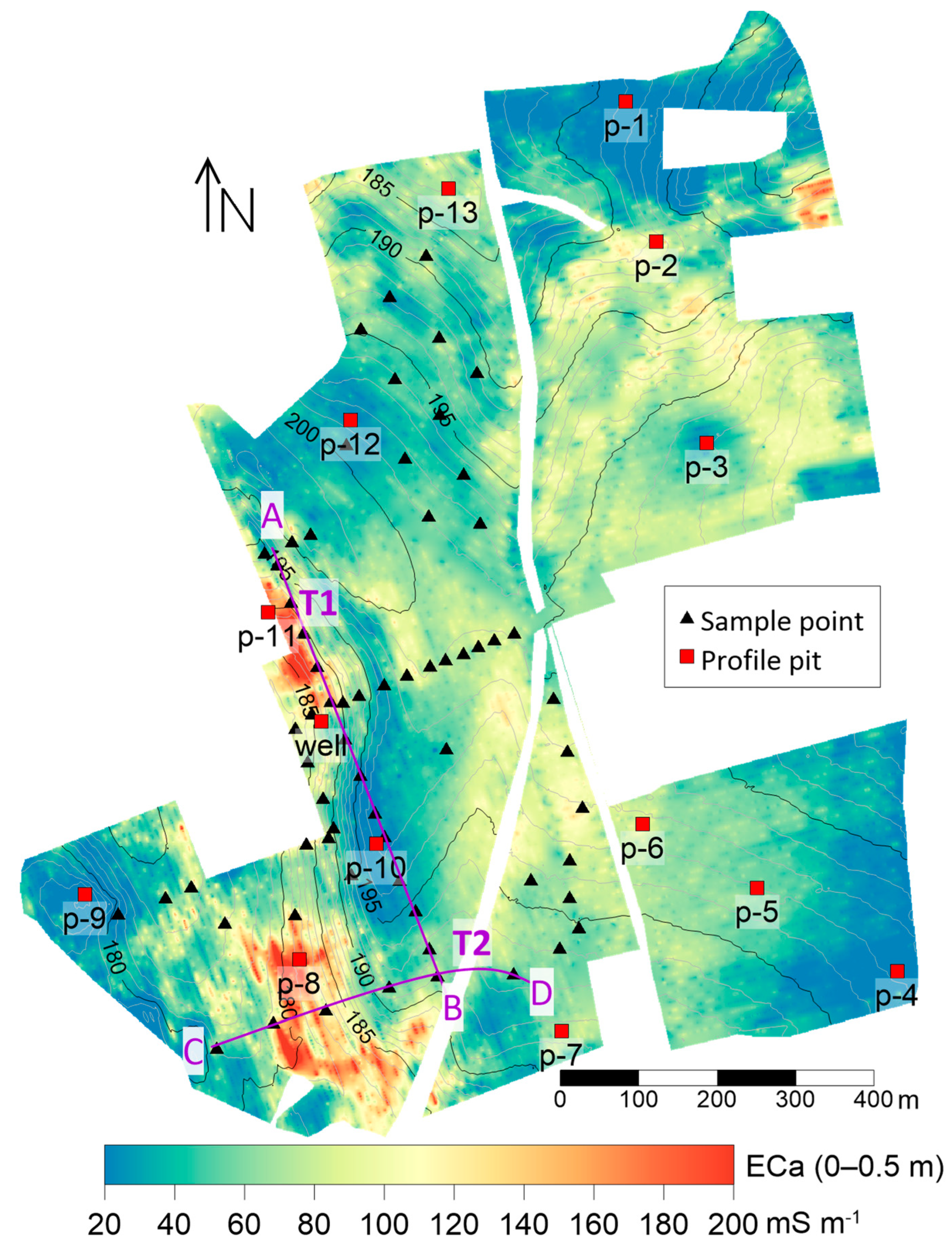
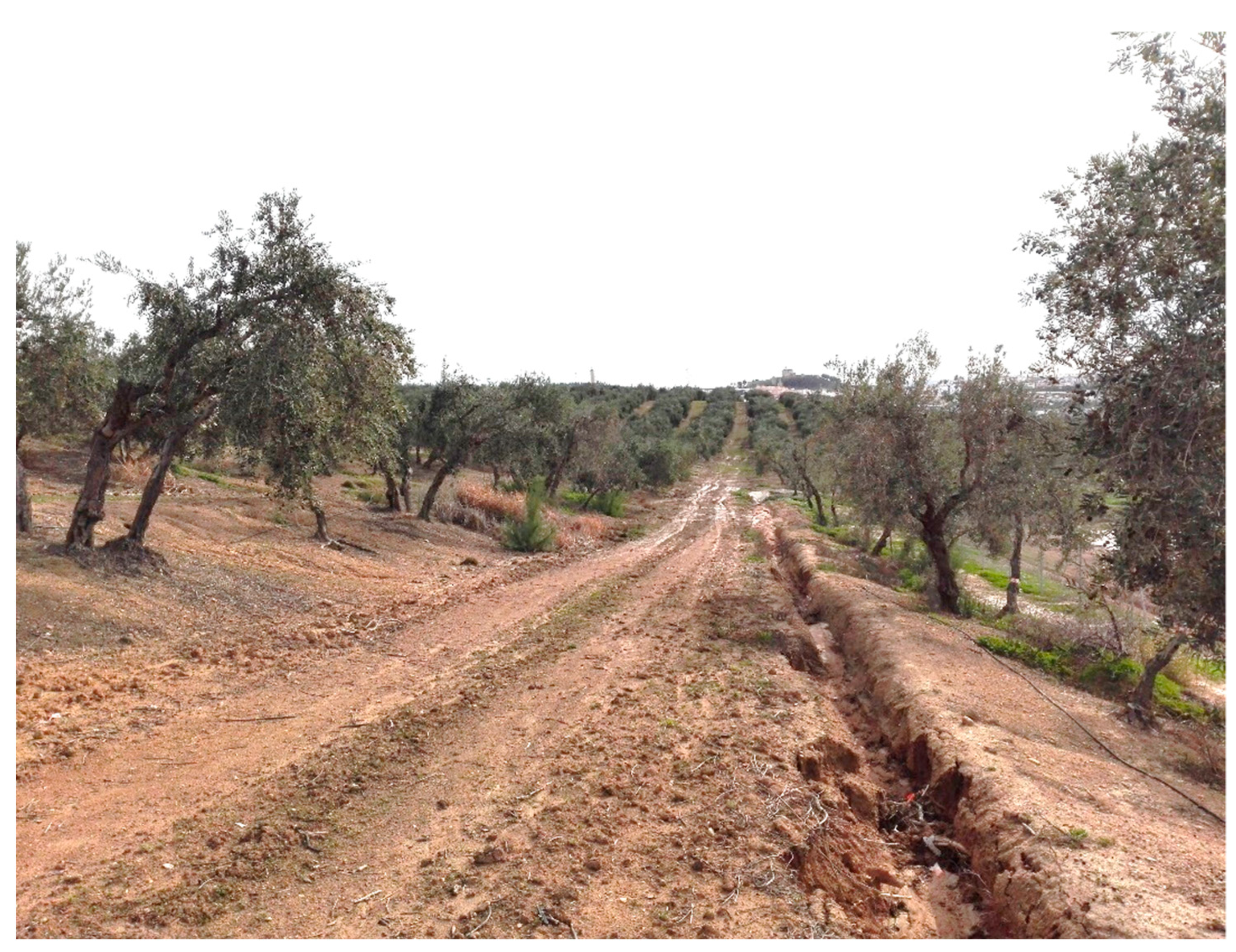
2.1. Study Site Description

This study was carried out in an olive grove (120 ha, 226 m above mean sea level), located in southern Spain, with trees planted in the early 1960s on a 12 × 10 m frame. The plot has been irrigated since 2012 with reclaimed saline water (EC ≈ 6 dS m⁻¹) from a nearby table olive processing plant. Irrigation was scheduled according to local practice and based on the FAO methodology [19]. The soils developed on the calcareous material belong to the great group of Calcixerepts, although Haploxererts and Xerofluvents are also found [20]. The climate is temperate Mediterranean with dry and hot summers (Csa), according to the Köppen classification [21]. Eighty percent of the mean annual precipitation (662 mm) occurs between October and March, with practically no rainfall between June and August, due to the Atlantic coastal influence. The average temperature is 17.1 °C, with the highest average monthly temperature (25.7 °C) occurring in July and the lowest (9.9 °C) in December.

2.2. Field Measurements

In this work, we summarize the combined results from field work conducted in a commercial olive grove between 2013 and 2017, within the context of different projects and field campaigns. Total rainfall for the hydrological years from 2013/14 to 2017/18 was 388, 410, 473, 410, and 757 mm, respectively, yielding an average annual rainfall of 488 mm. Average annual ETo was 1286 mm. Different measurement locations and techniques were used and combined in a unique data set, which is presented here. In November 2013, a preliminary exploration of the farm was carried out with an electromagnetic induction sensor. Based on the ECa maps resulting from these measurements, the location of 13 profile pits was chosen (Figure 1), for which a complete description of the soil profile was made in June 2014. In addition, samples were taken from the groundwater that emerged at the bottom of several profile pits. At these locations, piezometers were installed, and water level and quality were measured on seven different days, ending in July 2015. Water level below the soil surface was manually measured, and water samples were extracted using a using a 12 V peristaltic pump. Near the profile pits, paired topsoil samples (0–0.2 m) were taken in between the tree rows and under the drippers in the tree rows in June 2014 and analyzed in the laboratory for 1:5 soil–water solution extract conductivity (EC_1:5) and Exchangeable Sodium Percentage (ESP) [22] to evaluate the extent of the local effects of the effluent irrigation. Based on the results of the first evaluation of the farm (2013–2014), smaller irrigation volumes were recommended, resulting in the implementation of a more conservative irrigation strategy from 2015 onwards. To check the effect of this change on the soil salinity, another ECa survey was performed in February 2017, with the same electromagnetic induction sensor. The total rainfall and ETo between both ECa surveys were 1470 and 3990 mm, respectively. After this survey, taking advantage of the installation works of a new irrigation system in the field, soil samples were taken on 27 July, 22 November, and 21 December 2017 at 65 locations (Figure 1), with intervals of 0.3 m to a depth of 1.2 m, and analyzed in the laboratory for saturated paste extract electrical conductivity (ECe) and EC_1:5, according to the methodology presented by [22], clay (hydrometer method), and carbonate content (calcimeter method). The sodicity hazard was assessed by the Sodium Adsorption Ratio (SAR), which refers to ion concentrations in the soil solution and is calculated, according to [22], as SAR $=\left[N{a}^{+}\right]/{\left[\left(\left[C{a}^{2+}\right]+\left[M{g}^{2+}\right]\right)/2\right]}^{0.5}$, with the cation concentrations of the saturated paste extract in mmol_c L⁻¹ measured using a PinAAcle500 atomic adsorption spectrofotometer (Perkin Elmer, Waltham, MA, USA). The Exchangeable Sodium Percentage (ESP) refers to the adsorbed ions on the soil exchange surfaces. Ref. [23] showed that for practical field applications (SAR < 30 mmol_c^1/2 L^−3/2) ESP ≈ SAR.

2.3. ECa Measurement and Inversion

ECa was measured with a DUALEM-21S electromagnetic induction sensor (Dualem Inc., Milton, Canada). The sensor consists of a coil that transmits an electromagnetic field at low frequency (9 kHz) and two pairs of receiver coils with horizontal and perpendicular orientations with respect to the transmitter. The distance between the emitting coil and the receivers with perpendicular orientation is 1.1 and 2.1 m, resulting in theoretical depths of exploration (DOEs) of 0–0.5 m and 0–1.0 m, respectively. The horizontally oriented receivers are located at distances of 1 and 2 m from the emitter, with DOEs of 0–1.5 m and 0–3.0 m, respectively. The sensor is integrated in a mobile platform consisting of an all-terrain vehicle (ATV) equipped with a GPS-RTK positioning system that drags the PVC sled in which the DUALEM-21S is housed. The measurements were performed at speeds ranging from 5 to 10 km/h along the lanes in between the tree lines. At each measurement point, the four values of ECa corresponding to the above indicated DOEs were recorded. The measured ECa is the integrated EC of a bulk soil volume and depends, therefore, not only on soil salinity, but also on other soil properties such as clay or water content, among others. Therefore, it is necessary to determine, for each application, which soil properties predominate in their contribution to the ECa signals [12].

The raw ECa data were filtered for outliers, and spatial consistency was checked. The presence of conductive elements such as metal pipes or fence elements may result in anomalous ECa measurements. In addition, sensor tilting and rotation, because of rough soil surface conditions during measurement, can change the coil configuration with respect to the soil surface and produce erroneous measurements. Subsequently, the ECa measurements were interpolated on a 1 × 1 m grid. Descriptive statistics and cumulative distribution functions (cdfs) of interpolated ECa and ECa increments from 2013 to 2017 (∆ECa = ECa₂₀₁₇ − ECa₂₀₁₃) were provided. To quantify the spatial evolution of the ECa across the farm, we use as an indicator the probability of exceeding a certain value of (∆ECa).

The four ECa signals were then inverted using the EM4Soil code (EMTOMO, Lisbon, Portugal) to obtain the vertical distribution of the “true” conductivity, σ. EM4Soil provides pseudo two- or three-dimensional images of σ, conditioned on neighboring σ values, close to the estimated point. According to the smoothing condition imposed on the σ profile, two inversion algorithms (S1 and S2) were considered. Both are variations of the Occam regularization method [24], though the S2 inversion algorithm produces smoother results than S1. Given the high ECa observed in this field, the inversion was performed using the full solution (FS) for a range of values of the damping factor, λ. More details on the inversion algorithm can be found in [16].

3. Results and Discussion

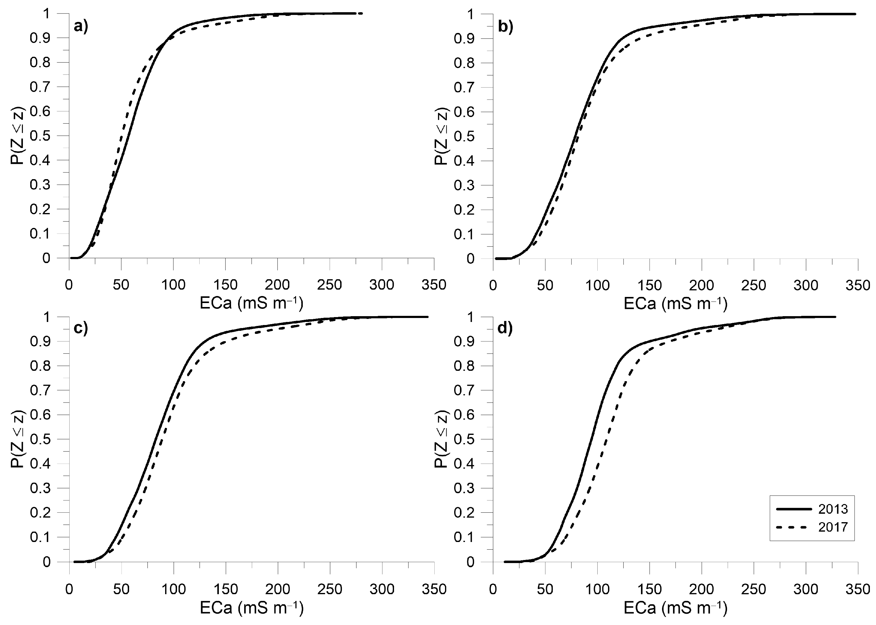
3.1. Spatial Distribution of ECa in 2013 and 2017

The ECa data from 2013 provided information on the horizontal and vertical distribution of soil salinity across the grove. Large ECa values were detected in depressions at the foot of steeply sloping areas (Figure 1) and are indicative of salt accumulation as a result of surface and subsurface water flow.

Table 1. Descriptive statistics of the four ECa signals measured in 2013 and 2017. DOE: depth of exploration, n: number of measurements, m: mean, s: standard deviation, CV: coefficient of variation, k and λ: fitted Weibull scale and shape parameters, respectively.

DOE	Year	n	m	s	CV	Skew.	Kurt.	Weibull
m			mS m−1					k	λ	R2
0–0.5	2013	31,677	59.8	36.5	0.61	1.43	6.11	67.2	2.33	0.984
	2017	81,806	58.8	35.0	0.60	1.98	8.49	65.4	2.31	0.940
0–1.0	2013	31,306	84.2	45.0	0.53	1.55	6.61	93.0	2.70	0.968
	2017	78,921	88.3	44.0	0.50	1.61	6.94	100.0	2.60	0.955
0–1.5	2013	31,677	90.7	45.8	0.51	1.48	6.15	98.1	2.78	0.963
	2017	81,806	97.3	45.2	0.46	1.47	6.22	108.8	2.76	0.953
0–3.0	2013	31,306	106.1	46.8	0.44	1.50	5.62	112.7	3.26	0.900
	2017	78,921	114.2	42.5	0.37	1.24	5.39	127.1	3.38	0.941

and Figure 2 show that ECa increased with DOE throughout the field, particularly in areas of high ECa (>125 mS m⁻¹), corresponding to 10–15% of the area of the olive grove.

Both the larger ECa (>200 mS m⁻¹) observed for the deepest DOEs and the positive skewness of the probability density functions (pdfs) are indicative of the artificial accumulation of conductive material between 1 and 3 m deep (Table 1 and Figure 2). The decrease in the coefficient of variation (CV) with DOE indicates that this conductive material was distributed more homogeneously in the subsoil than in the proximity of the surface. This can also be seen in the decreasing skewness with DOE, particularly in 2017. This, together with the slight increase in mean ECa (Table 1) from 2013 to 2017 (except for the shallowest DOE), shows that the accumulation of conductive material in the subsoil persisted during this period, despite the implementation of a more conservative irrigation strategy since 2015. In order to check the robustness of this interpretation, the scale (k) and shape (λ) parameters of the fitted Weibull distribution are also provided in Table 1. Parameter k increased from 2013 to 2017 for all DOEs, except for 0–0.5 m, while λ was inversely related to the skewness, with values near 3 indicating near-normal distributions.

For the 0–0.5 m signal, ECa decreased between 2013 and 2017 only in areas with intermediate values (50–100 mS m⁻¹), while, for deeper DOE’s, ECa increased for practically the entire data range (Figure 2). The environmental conditions during both surveys might have influenced the differences observed in Figure 2. The soil temperature at 0.6 m depth was 5 °C higher in November 2013 (19 °C) than what was measured at the same depth in February 2017 (14 °C), which theoretically causes a 10% increment in ECa measured in 2013 compared to 2017 [25]. To account for temperature effects, it is generally recommended to correct the ECa data to a reference temperature (e.g., 25 °C). Yet, soil temperature varies both vertically and laterally, making the implementation of such corrections in field studies cumbersome. Note that by accounting for soil temperature effects, the increment for ECa between 2013 and 2017 was expected to become larger (Table 1 and Figure 2). Therefore, the temperature correction can be omitted without compromising the main findings of this study.

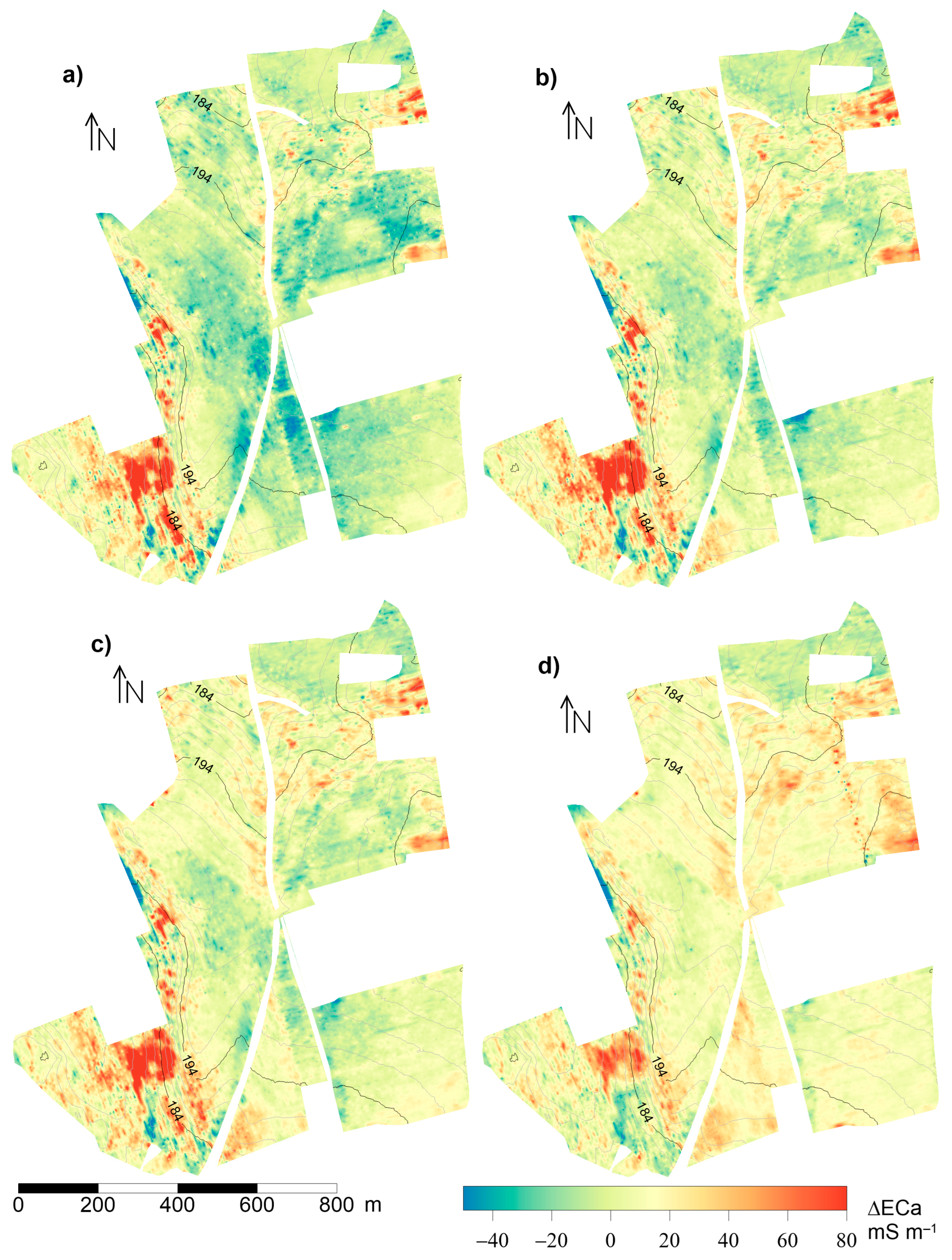
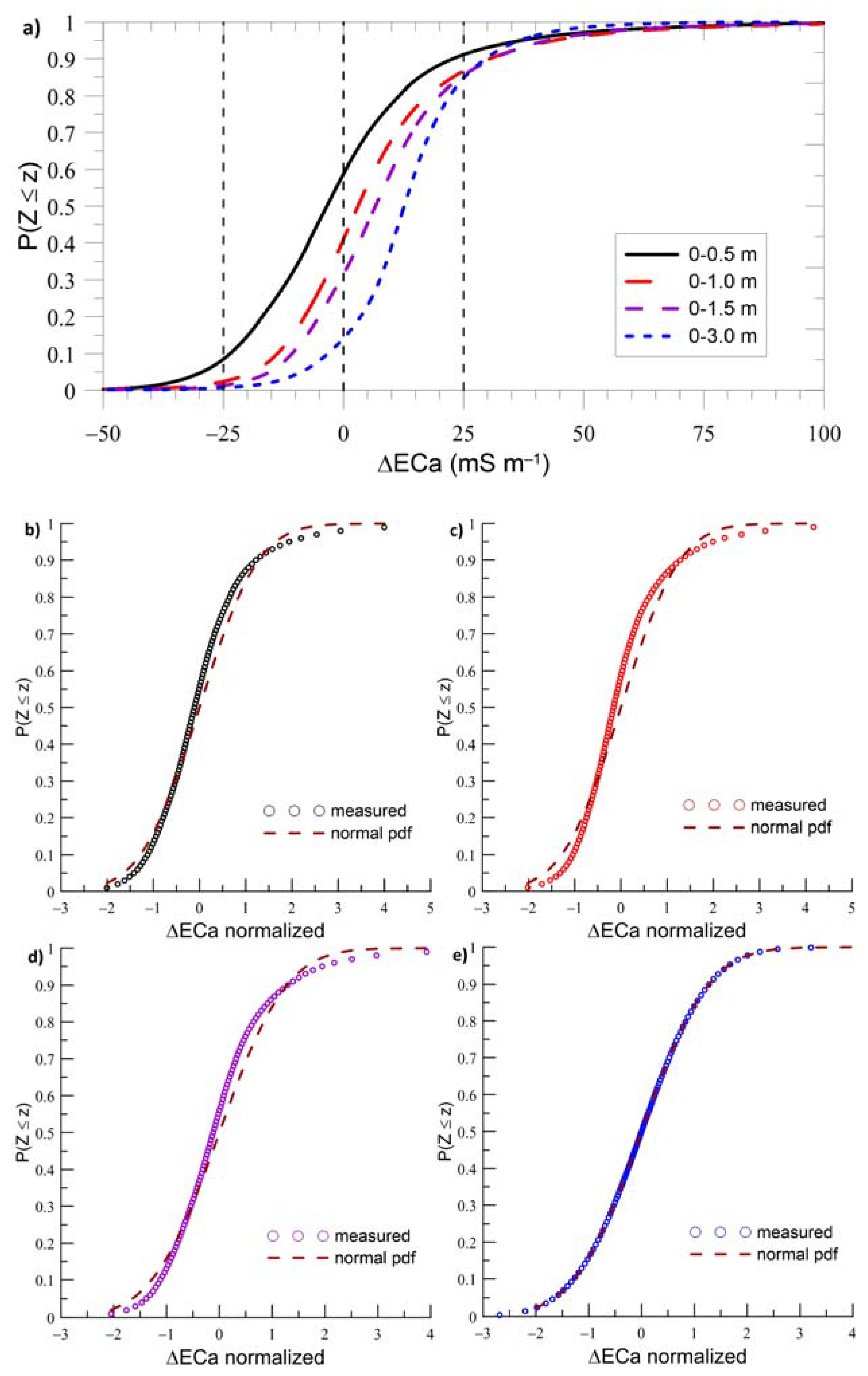
3.2. Spatial Distribution of ΔECa

∆ECa showed a similar spatial pattern for the four signals (Figure 3). The largest ∆ECa (>60 mS m⁻¹) were observed in areas with the highest ECa (Figure 1). In large areas of the farm, ECa decreased (∆ECa < 0), particularly for the shallowest DOE, possibly because of the changes introduced in the irrigation management from 2015 onwards. Despite the generalized increments observed for the deepest signal (0–3.0 m), the largest ∆ECa values were smaller than those observed for the other shallower signals. This is also evident from the comparison of the ∆ECa cdfs for the four signals in Figure 4, which show that, for ∆ECa > 35 mS m⁻¹, the cumulative probability of the deepest signal exceeds that of the other signals, indicating a lower probability of occurrence of the largest ∆ECa values for the 0–3.0 m signal. This is also in agreement with the good fit of the normal distribution for the deepest ∆ECa signal.

To assess the importance of the different measurement conditions in 2013 and 2017, such as the soil temperature and water content, threshold values of −25, 0, 25, and 50 mS m⁻¹ were considered to identify the proportion of the areas where the ECa increased or decreased (

Table 2. Probabilities, P (Z ≤ z), of the increments in ECa between 2013 and 2017 for the four signals.

P (Z < z)	0–0.5 m	0–1.0 m	0–1.5 m	0–3.0 m
z = 50 mS m−1	0.971	0.962	0.966	0.985
z = 25 mS m−1	0.911	0.866	0.854	0.847
z = 0 mS m−1	0.587	0.409	0.315	0.141
z = -25 mS m−1	0.085	0.024	0.013	0.007

). For the shallowest signal (0–0.5 m), ECa increased by more than 25 mS m⁻¹ in approximately 9% of the olive grove area, while, for the other signals, this proportion was near 15%. Considering the ∆ECa > 50 mS m⁻¹ threshold (Table 2), the ratio was 1.5% for the deepest signal (0–3.0 m) and approximately 3% for the other signals. These results indicate that the shallow and deep ECa in the areas of high ECa (Figure 1) were controlled by different mechanisms and that the ∆ECa reflected changes in the conductive material present in the subsoil at different depths. For the surface signal (0–0.5 m), ECa decreased between 2013 and 2017 by more than 25 mS m⁻¹ (∆ECa < −25 mS m⁻¹) in 8.5% of the grove, while the other signals showed decreasing proportions, between 2.7% and 0.7%, with DOE.

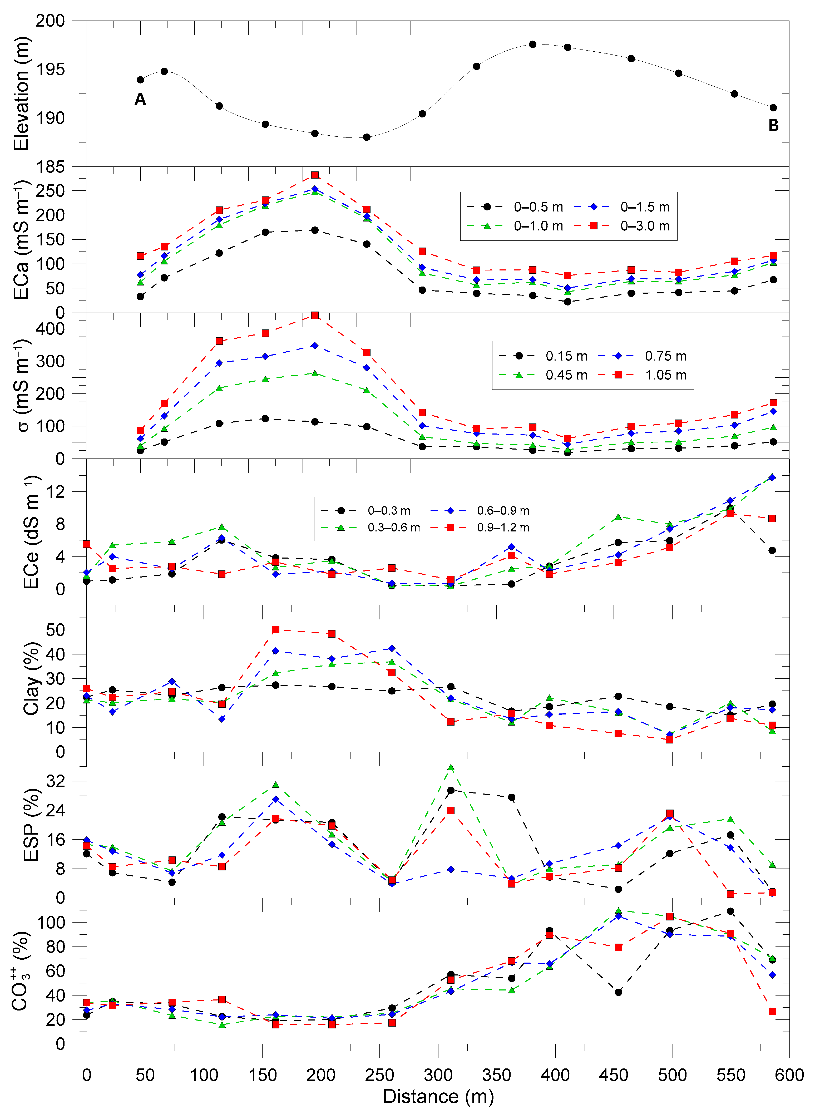
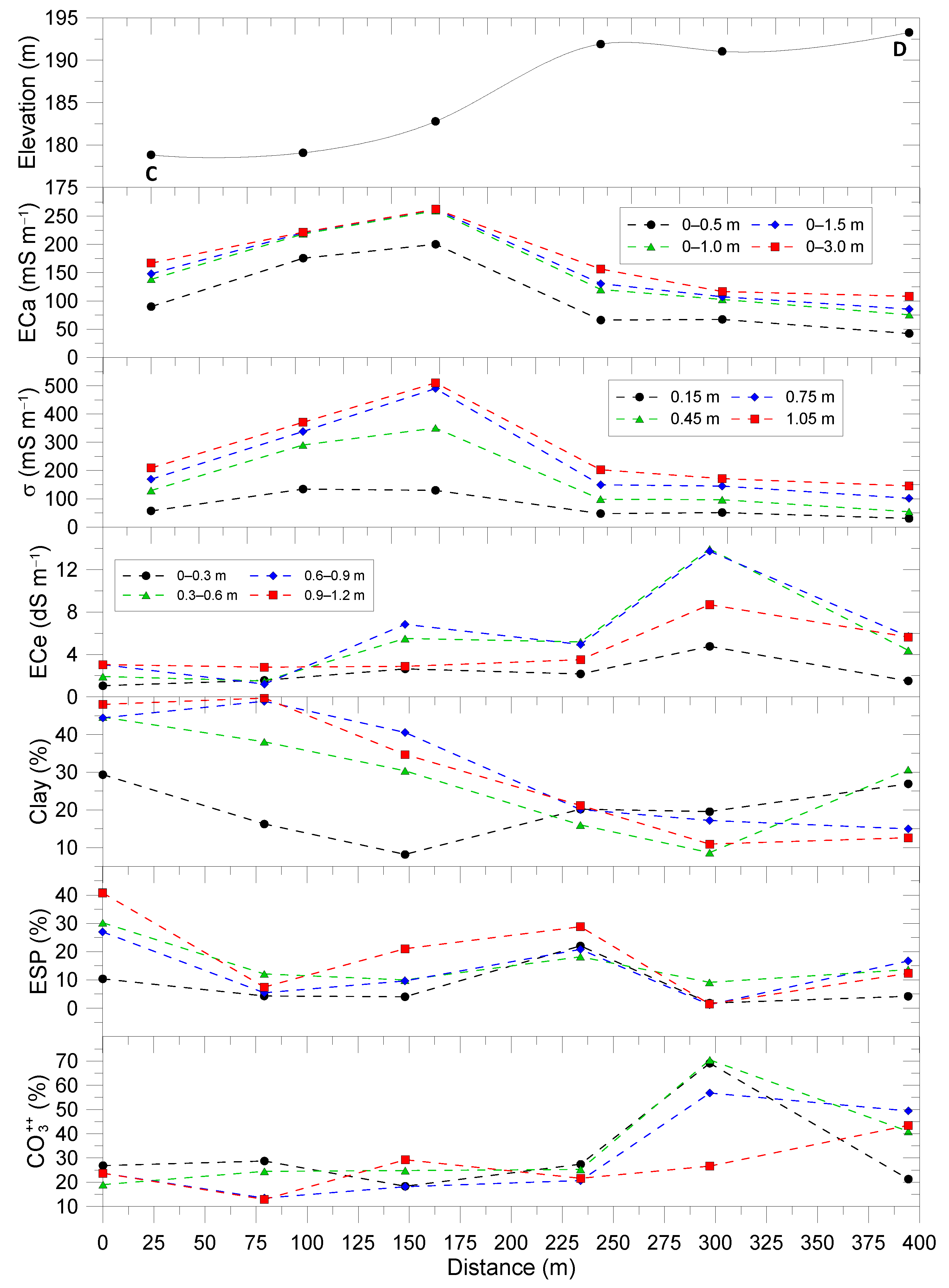
3.3. Soil Data and Relationship with the ECa

The results of the laboratory analysis of soil and water samples extracted from the piezometers between June 2014 and July 2015 confirmed the existence of apparently independent perched water tables, with varying quality according to the cropping season. Figure 5 shows that minimum EC values were reached toward the end of spring, as a result of the dilution of the soil solution by winter and spring rains and the absence of irrigation with saline reclaimed water, to reach maximum values in summer as a result of irrigation and the effects of the high evaporation rates. This is particularly evident for p-8 (see Figure 1), located in an area of high ECa. The lack of good drainage conditions, possibly because of the increasing clay content with depth, reaching 50–60% at p-8 (data not shown), can contribute to the formation of perched water tables in this area, as in other areas of the farm where a high ECa was observed. For comparison, the ECs measured in June 2014 in the creek near the northern limit of the grove, in the vicinity of p-13, and in the well (Figure 1) are provided in Figure 5. Considering the ECs of these waters in combination with their SAR, which varied between 5 and 10 (mmol_c^1/2 L^−3/2), and according to the classification proposed by [20] or [23] for soil salinity and sodicity hazard, their use for irrigation purposes should not pose any risk. Leaf analysis performed in October 2014 and May 2015 in the surroundings of the piezometers revealed no negative effects from irrigation with saline wastewater.

The application of the effluent was especially noticeable under the drippers, where mean ESP and pH were significantly higher than in the lanes (22.5% and 8.2%; 8.9 and 8.2, respectively), while the difference in the mean EC_1:5 in the lanes and under the drippers was not significant (Figure 6a,b). This shows that ESP might be a better indicator for soil salinization in this context, with Na-rich irrigation water. Large amounts of other cations were already present in these soils before irrigation started, making EC_1:5 less effective at detecting salinization effects of the irrigation with regenerated wastewater. It is also remarkable that the effect of irrigation on ESP is noticed in the lanes, several meters away from the drippers. This might be a consequence of local surface runoff, away from the drippers toward the center of the lanes, which is produced by overirrigation or broken irrigation pipes. This can be clearly observed in Figure 6a, with similar ESP values under the drippers and in the lanes for three points.

The ECa measured in 2013 along the lanes showed a clear relationship with soil salinity (Figure 6c,d). Linear relationships were found for EC_1:5 and ESP with the ECa (0–0.5 m) measured in the lanes, with R² = 0.69 and 0.68, respectively. This is indicative of the potential of EMI for the spatial evaluation of both parameters at the field or farm scale. These relationships are lost, however, when EC_1:5 and ESP data, which are measured under the drippers and not in the lanes where the ECa measurements were performed, are considered.

Figure 7 shows the classification of the soil samples taken in 2017 (Figure 1) according to ESP, ECe, and pH. The proportion of “non-saline” and “non-sodic” samples ranged from 36% (0.3–0.6 m) to 56% (0–0.3 m), with pH values generally above 8.5. Samples classified as “saline” (ECe > 4 dS m⁻¹ and ESP < 15%) represented between 14% (0–0.3 m) and 30% (0.6–0.9 m) of the total, while the “sodic”, with pH < 8.5, and “alkaline” samples, with pH > 8.5, (ECe ≤ 4 dS m⁻¹ and ESP ≥ 15%) represented between 8% (0.6–0.9 m) and 22% (0–0.3 m). These last two categories imply an excessive presence of Na in the soil solution, with respect to the concentration of other cations that potentially leads to a loss of soil structure and limitation of soil water retention and transmission, particularly in combination with low ECe and high pH (near 10, at some points).

This sample classification is not maintained for the different depths analyzed nor does it show clear spatial patterns. The occurrence, apparently random, of the different categories of affectation by Na could be a consequence of the deterioration of the irrigation system, with frequent ruptures of the pipes at different points of the farm and the progressive obstruction of the drippers as a result of irrigation with the reclaimed water, as observed during the field work. This would result in a heterogeneous distribution of irrigation water across the grove and provides an explanation for the results shown in Figure 7.

3.4. Inversion

The results of the three-dimensional inversion provide more detail for the vertical distribution of the conductivity than the raw ECa data. Figure 8 shows σ for different depths in the western part of the olive grove, estimated using the 2017 ECa measurements. It can be seen how, in the areas of high ECa (Figure 1), σ increases with depth to reach maximum values near 0.8–1.0 m. From 1.2 m, σ decreases, until it reaches minimum values at 2.5 m. This indicates the presence of conductive material at 1 m depth, possibly corresponding to the perched saline water tables that were characterized in Figure 5. From 3 m depth, σ increases again, reaching very high values throughout the field at 4 m depth, which corresponds to the underlying water table that also shows a high salinity, according to the analytical results of the well water (Figure 5).

A two-dimensional inversion was made along transects T1 A–B and T2 C–D (see Figure 1), both with important topographic gradients and crossing areas of high ECa. The trends observed in these transects can, therefore, be considered representative for the entire olive grove (Figure 9). ECa and σ reached maximum values in the depression along the northern half of T1. Except for the high clay content that characterizes the soil profile in this zone, none of the other soil variables represented in Figure 9 can explain the observed trends in ECa and σ. Therefore, we attribute the high ECa and σ in the depression to higher soil water contents at the time of measuring the ECa, as evidenced by the signs of waterlogging that appear in the photograph in Figure 10. Although the ECe was high throughout the transect, and in particular near the southern end (B), the ECa (and σ) did not follow this trend and was possibly mimicked by the variation in soil water content or other soil properties. Since the soil water content was the lowest at the highest elevation of the transect (the southern half), not all the salts present in the soil solution are dissolved and detected by electromagnetic induction sensing. This could explain the smaller values of ECa and σ along this section of the transect, as compared to the northern half. In spite of this, a similar increasing trend toward endpoint B can be observed for ECe and ECa (and σ).

Similar trends were observed for transect T2 C–D, as shown in Figure 11. In this case, the maximum values of ECa and σ are larger than in transect T1. The similarity of the values for σ at 0.75 and 1.05 m depths may indicate the presence of local saline perched water tables (Figure 5) at these depths near the foot of the hillslope. Moreover, in this transect, maximum values of ECe, especially at depths between 0.3 and 0.9 m, were observed where the elevation was the highest. This occurred particularly at the second point from endpoint D, which coincided with the southern end (B) of transect T1 (Figure 9). The smaller water content of the soil profile at this point, located at a higher elevation, can again explain why the high ECe is not reflected in the ECa or the σ data. However, the ESP at this point is low, indicating a balance between the concentration of Na and the other cations of the soil solution in spite of the high ECe.

The apparent mismatch between the ECa measured in 2017 and the soil properties shown in Figure 9 and Figure 11 possibly has its origin in the vertical and lateral variations of soil moisture across the olive grove, because of the local terrain and variable soil conditions (clay content varied between 10% and 50%), in addition to deficiencies in the functioning of the irrigation system. Soil sampling was carried out according to the possibilities of access to the farm during the period July–December 2017. It is possible that, during this period, the soil conditions changed from the situation in February 2017, when the ECa measurements were made.

4. Conclusions

Irrigation with Na-rich regenerated wastewater from the olive processing industry produced local (drippers/lanes) and field-wide effects. This involved lateral superficial or subsuperficial water flows and transport of salts, according to local topographical conditions and soil composition and state. The initial EMI measurement in 2013 detected high values of ECa in the areas at the foot of the slopes, indicative of the accumulation of salts in these areas. ECa increased with the DOE, doubling for the deeper signal the ECa values of the shallower signal. The second measurement of ECa, in 2017, after the adoption of a more conservative irrigation strategy, showed a similar spatial pattern. In large areas (~50%) of the olive grove, a slight decrease in the ECa was observed, particularly for the most superficial signals, but in the areas of greater ECa an increment of more than 60 mS m⁻¹ was observed for the deeper signals. In general, increments of more than 25 mS m⁻¹ were measured in 15% of the olive grove.

The soil and water quality monitoring performed between 2014 and 2015 showed the existence of apparently independent saline perched water tables, at different locations across the olive grove, coinciding with the areas of high ECa, as identified in the measurements of 2013 and 2017. EC_1:5 and ESP measured in 2014, in the topsoil in the lanes, showed a linear relationship with the ECa measured in 2013, highlighting the potential of the EMI method for estimating these parameters.

Estimates of σ, made with an inversion code for producing three- and two-dimensional images from the ECa data, confirmed the presence of perched saline water tables and allowed us to more accurately estimate the water table depth. However, it was not possible to relate the ECa measured in 2017 and the estimated σ with the soil properties that were measured during the summer and autumn of 2017, possibly as a result of changes in field conditions and a heterogeneous distribution of soil water content that constitutes a factor of distortion in the relationship between ECa and ECe.

The results of this work indicate that the agricultural application of reclaimed saline water from the table olive industry can be carried out in this soil without serious problems. However, the practice requires continuous monitoring of the properties of irrigation water and soil quality to ensure its sustainability in the medium and long term. The results also confirm the potential of EMI tomography to perform such monitoring at the field or farm scale. Yet, the successful estimation of soil properties indicative of salinity will depend mainly on the possibilities of minimizing the influence of other soil properties that also influence ECa, such as moisture, clay content, or soil temperature.

References

1. Huertas-Alonso, A.J.; Gonzalez-Serrano, D.J.; Hadidi, M.; Salgado-Ramos, M.; Orellana-Palacios, J.C.; Sánchez-Verdú, M.P.; Xia, Q.; Simirgiotis, M.J.; Barba, F.J.; Dar, B.N.; et al. Table olive wastewater as a potential source of biophenols for valorization: A mini review. Fermentation 2022, 8, 215. [Google Scholar] [CrossRef]
2. Assouline, S.; Russo, D.; Silber, A.; Or, D. Balancing water scarcity and quality for sustainable irrigated agriculture: Balancing water scarcity and quality for irrigation. Water Resour. Res. 2015, 51, 3419–3436. [Google Scholar] [CrossRef]
3. Hopmans, J.W.; Qureshi, A.S.; Kisekka, I.; Munns, R.; Grattan, S.R.; Rengasamy, P.; Ben-Gal, A.; Assouline, S.; Javaux, M.; Minhas, P.S.; et al. Critical knowledge gaps and research priorities in global soil salinity. In Advances in Agronomy; Elsevier: Amsterdam, The Netherlands, 2021; Volume 169, pp. 1–191. ISBN 978-0-12-824590-3. [Google Scholar]
4. International Olive Council. The World of Table Olives. Available online: www.internationaloliveoil.org/the-world-of-table-olives (accessed on 14 June 2022).
5. Rincón-Llorente, B.; De la Lama-Calvente, D.; Fernández-Rodríguez, M.J.; Borja-Padilla, R. Table olive wastewater: Problem, treatments and future strategy. A review. Front. Microbiol. 2018, 9, 1641. [Google Scholar] [CrossRef] [PubMed]
6. Assouline, S.; Kamai, T.; Šimůnek, J.; Narkis, K.; Silber, A. Mitigating the impact of irrigation with effluent water: Mixing with freshwater and/or adjusting irrigation management and design. Water Resour. Res. 2020, 56, e2020WR027781. [Google Scholar] [CrossRef]
7. Murillo, J.M.; López, R.; Fernández, J.E.; Cabrera, F. Olive tree response to irrigation with wastewater from the table olive industry. Irrig. Sci. 2000, 19, 175–180. [Google Scholar] [CrossRef]
8. Melgar, J.C.; Mohamed, Y.; Serrano, N.; García-Galavís, P.A.; Navarro, C.; Parra, M.A.; Benlloch, M.; Fernández-Escobar, R. Long term responses of olive trees to salinity. Agric. Water Manag. 2009, 96, 1105–1113. [Google Scholar] [CrossRef]
9. Aragüés, R.; Guillén, M.; Royo, A. Five-year growth and yield response of two young olive cultivars (Olea Europaea L., Cvs. Arbequina and Empeltre) to soil salinity. Plant Soil 2010, 334, 423–432. [Google Scholar] [CrossRef]
10. Pedrero, F.; Grattan, S.R.; Ben-Gal, A.; Vivaldi, G.A. Opportunities for expanding the use of wastewaters for irrigation of olives. Agric. Water Manag. 2020, 241, 106333. [Google Scholar] [CrossRef]
11. Visconti, F.; de Paz, J.M. Field comparison of electrical resistance, electromagnetic induction, and frequency domain reflectometry for soil salinity appraisal. Soil Syst. 2020, 4, 61. [Google Scholar] [CrossRef]
12. Doolittle, J.A.; Brevik, E.C. The use of electromagnetic induction techniques in soils studies. Geoderma 2014, 223–225, 33–45. [Google Scholar] [CrossRef] [Green Version]
13. De Carlo, L.; Vivaldi, G.A.; Caputo, M.C. Electromagnetic induction measurements for investigating soil salinization caused by saline reclaimed water. Atmosphere 2022, 13, 73. [Google Scholar] [CrossRef]
14. Pedrera-Parrilla, A.; Van De Vijver, E.; Van Meirvenne, M.; Espejo-Pérez, A.J.; Giráldez, J.V.; Vanderlinden, K. Apparent electrical conductivity measurements in an olive orchard under wet and dry soil conditions: Significance for clay and soil water content mapping. Precis. Agric. 2016, 17, 531–545. [Google Scholar] [CrossRef]
15. Scudiero, E.; Skaggs, T.H.; Corwin, D.L. Simplifying field-scale assessment of spatiotemporal changes of soil salinity. Sci. Total Environ. 2017, 587–588, 273–281. [Google Scholar] [CrossRef] [PubMed]
16. Triantafilis, J.; Monteiro Santos, F.A. Electromagnetic Conductivity Imaging (EMCI) of soil using a DUALEM-421 and inversion modelling software (EM4Soil). Geoderma 2013, 211–212, 28–38. [Google Scholar] [CrossRef]
17. Huang, J.; Nhan, T.; Wong, V.N.L.; Johnston, S.G.; Lark, R.M.; Triantafilis, J. Digital soil mapping of a coastal acid sulfate soil landscape. Soil Res. 2014, 52, 327. [Google Scholar] [CrossRef]
18. Huang, J.; McBratney, A.B.; Minasny, B.; Triantafilis, J. Monitoring and modelling soil water dynamics using electromagnetic conductivity imaging and the ensemble kalman filter. Geoderma 2017, 285, 76–93. [Google Scholar] [CrossRef]
19. Allen, R.G.; Pereira, L.S.; Raes, D.; Smith, M. FAO Irrigation and Drainage Paper No. 56; Food and Agriculture Organization of the United Nations: Rome, Italy, 1998. [Google Scholar]
20. Soil Survey Staff. Keys to soil taxonomy. Soil Conserv. Serv. 2014, 12, 410. [Google Scholar]
21. Peel, M.C.; Finlayson, B.L.; McMahon, T.A. Updated world map of the Köppen-Geiger climate classification. Hydrol. Earth Syst. Sci. 2007, 11, 1633–1644. [Google Scholar] [CrossRef]
22. Corwin, D.L.; Yemoto, K. Measurement of soil salinity: Electrical conductivity and total dissolved solids. Soil Sci. Soc. Am. J. 2019, 83, 1–2. [Google Scholar] [CrossRef]
23. Sposito, G. The Chemistry of Soils, 2nd ed.; Oxford University Press: New York, NY, USA, 2008; pp. 296–315. [Google Scholar]
24. deGroot-Hedlin, C.; Constable, S. Occam’s inversion to generate smooth, two-dimensional models from magnetotelluric data. Geophysics 1990, 55, 1613–1624. [Google Scholar] [CrossRef]
25. Ma, R.; McBratney, A.; Whelan, B.; Minasny, B.; Short, M. Comparing temperature correction models for soil electrical conductivity measurement. Precis. Agric. 2011, 12, 55–66. [Google Scholar] [CrossRef]
Figure 1. ECa (0–0.5 m) map of the experimental field, measured in 2013, with topography and locations of profile pits and sample points. Piezometers were installed at p-2, p-3, p-5, p-6, p-7, p-8, and p-13. Transects T1 (A,B) and T2 (C,D) are represented with continuous lines.
Water 14 03049 g001
Figure 2. Cumulative distribution functions of interpolated ECa measured in November 2013 and February 2017 for DOEs of (a) 0–0.5 m; (b) 0–1.0 m; (c) 0–1.5 m and (d) 0–3.0 m.
Water 14 03049 g002
Figure 3. Spatial distribution of the increments in ECa between 2013 and 2017 (∆ECa) for DOEs of (a) 0–0.5 m; (b) 0–1.0 m; (c) 0–1.5 m and (d) 0–3.0 m.
Water 14 03049 g003
Figure 4. (a) Cumulative distribution functions of the increments in interpolated ECa between 2013 and 2017 (∆ECa) for the four interpolated signals shown in Figure 3. Comparison with the normal distribution for DOEs of (b) 0–0.5 m; (c) 0–1.0 m; (d) 0–1.5 m and (e) 0–3.0 m.
Water 14 03049 g004
Figure 5. Daily rainfall and EC measured in the piezometers installed at the profile pits (indicated with prefix p in Figure 1), the well, and the creek in the northern part of the farm, from 22 June 2014 to 13 July 2015.
Water 14 03049 g005
Figure 6. Relationshipsbetween (a) ESP and (b) EC1:5 measured (0–0.2 m) under the drippers and in the lanes nearby the profile pits shown in Figure 1. Relationship of (c) ESP and (d) EC1:5, measured in the lanes and under the drippers (0–0.2 m), with the ECa (0–0.5 m) measured in the lanes in 2013. The discontinuous line represents the linear regression for the lane data.
Water 14 03049 g006
Figure 7. Classification of the samples taken in 2017 (Figure 1), according to the percentage of exchangeable sodium (PSI), the electrical conductivity measured in the saturated paste extract (ECe), and the pH for the four depths.
Water 14 03049 g007
Figure 8. Depth-specific distribution of the actual soil conductivity, σ (mS m−1), estimated by three-dimensional inversion of the ECa data measured in February 2017. The images correspond to depths ranging from 0.2 to 3.9 m.
Water 14 03049 g008
Figure 9. Elevation and different soil properties measured in 2017 along transect T1 A–B (Figure 1).
Water 14 03049 g009
Figure 10. Waterlogging in the lower area of transect T1 A–B (Figure 9). The photograph is taken looking toward point B.
Water 14 03049 g010
Figure 11. Elevation and different soil properties measured in 2017 along the transect T2 C–D (Figure 1).
Water 14 03049 g011