
Sentinel-1 and Sentinel-2 Data to Detect Irrigation Events: Riaza Irrigation District (Spain) Case Study
 , , , , , and
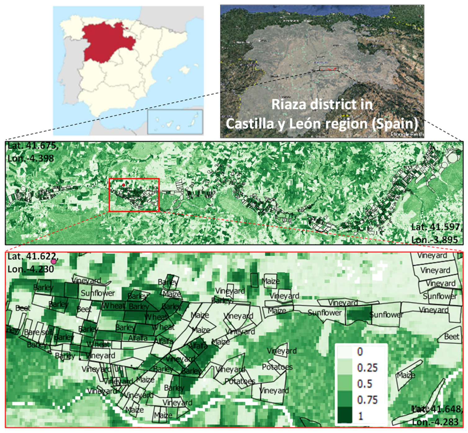
Abstract
:1. Introduction
2. Materials and Methods
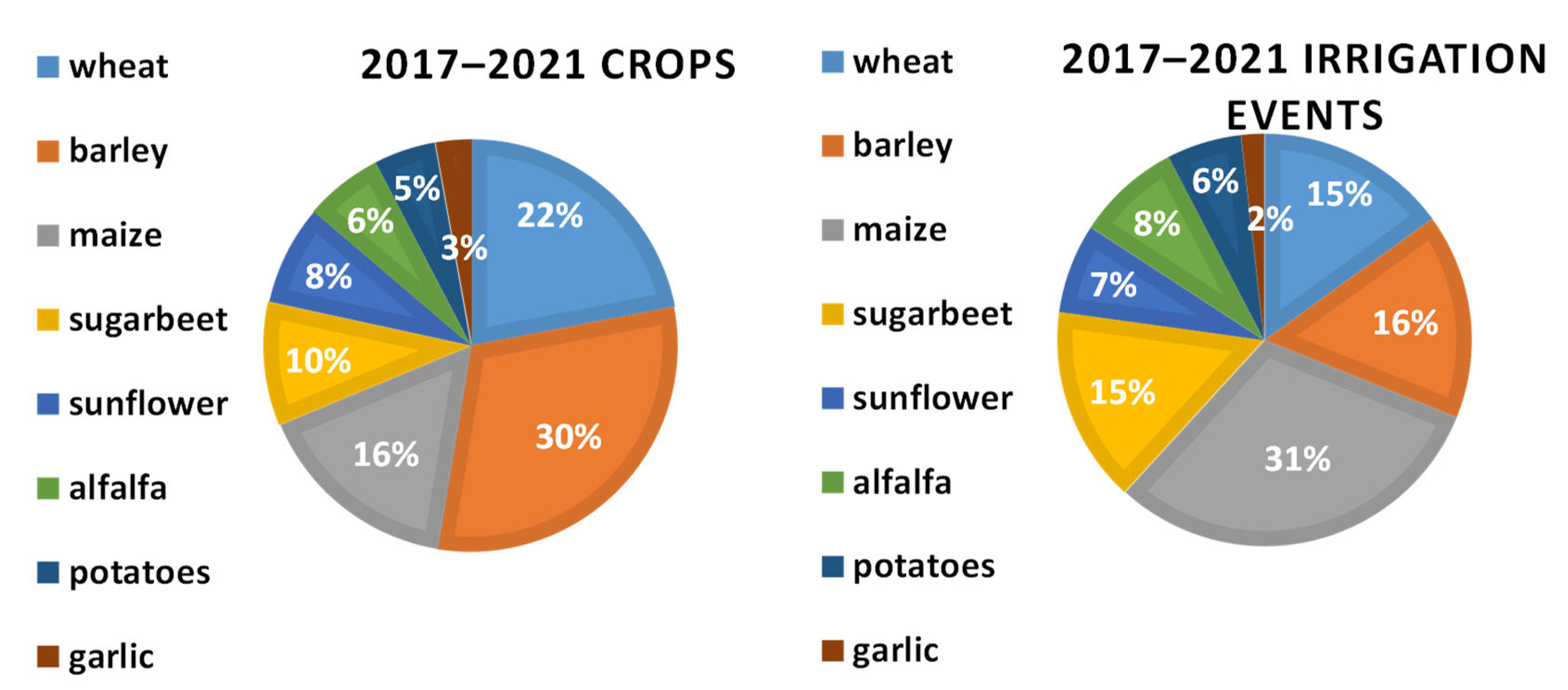
2.1. Test Site and Ground Data
2.2. Sentinel-1 and Sentinel-2 Data
2.3. Sentinel-1 and Sentinel-2 Surface Soil Moisture Maps
2.4. Why SSM for Irrigation Identification
2.5. Optimal Spatial Resolution for the SSM Contrast Detection
3. Results and Discussion
3.1. Causes of Incertitude in Mapping Irrigated Areas
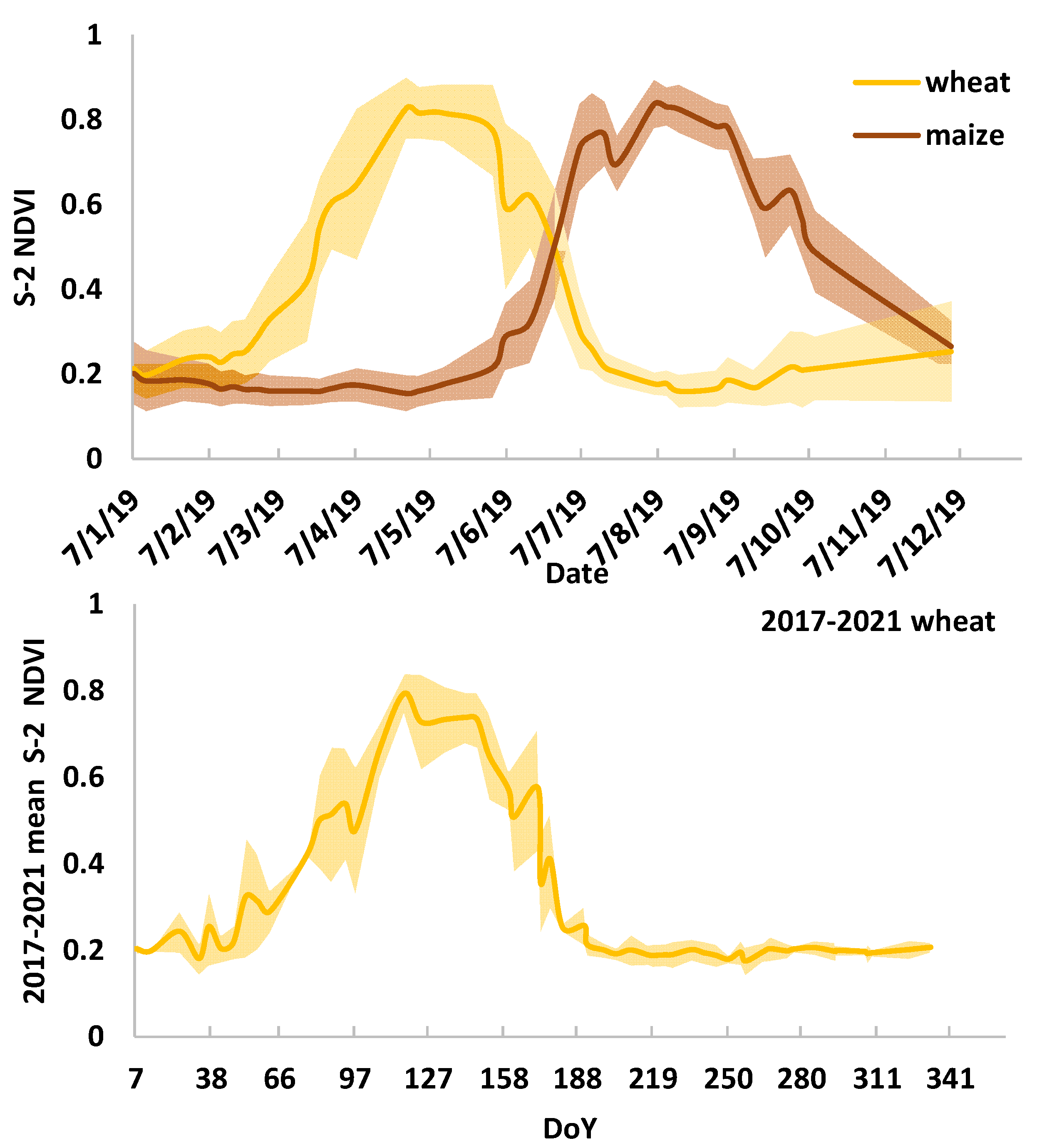
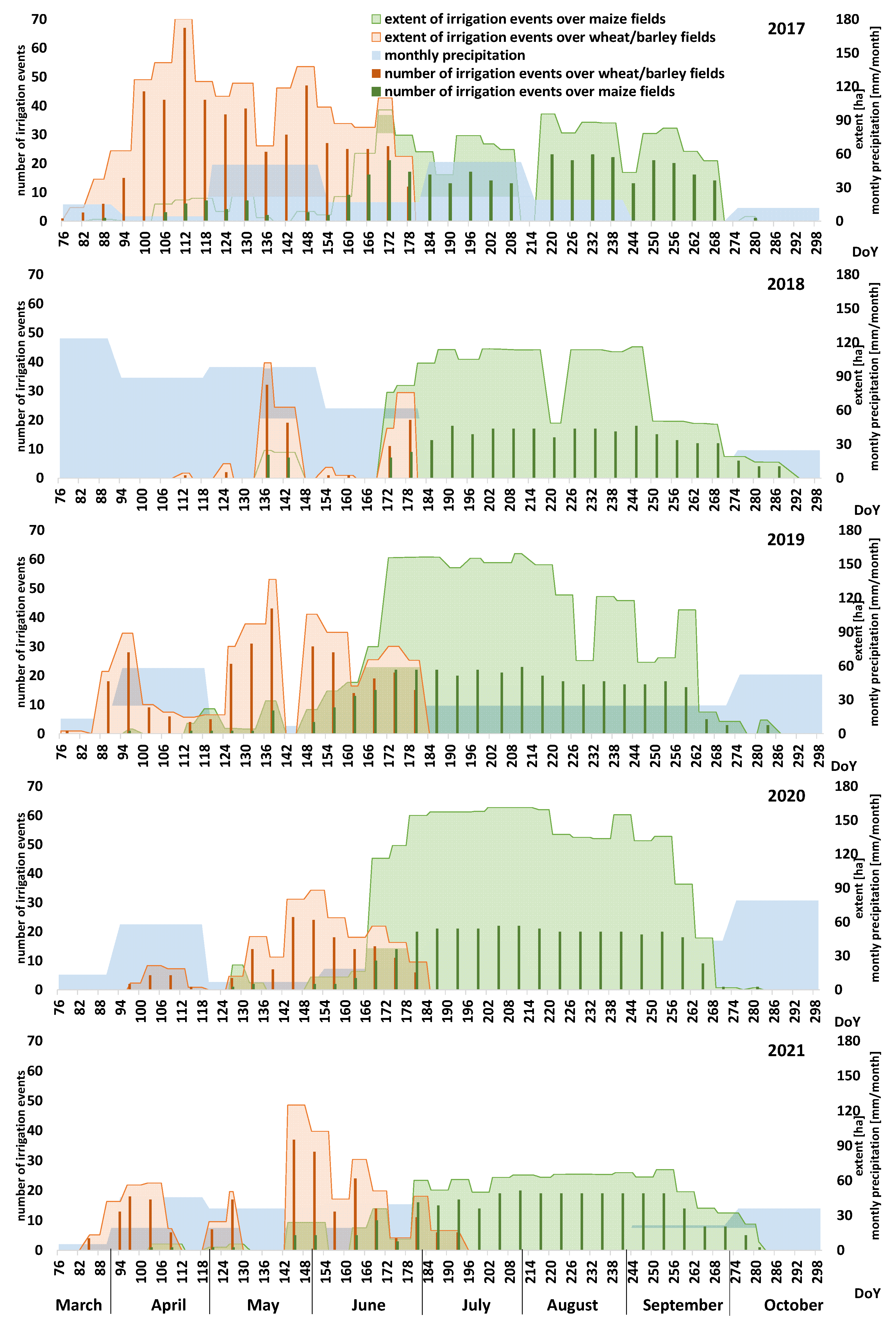
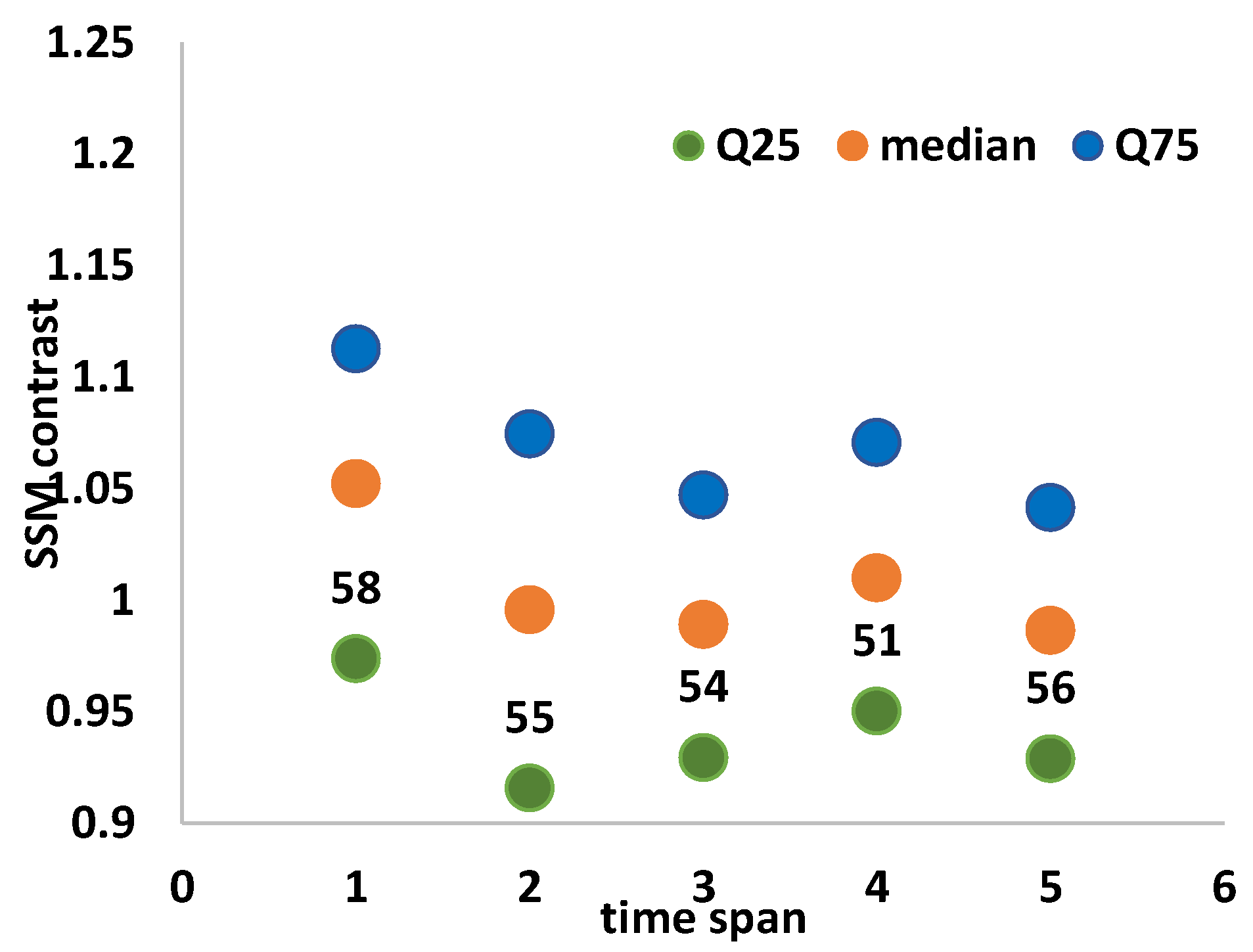
3.1.1. Effect of Irrigation Timing
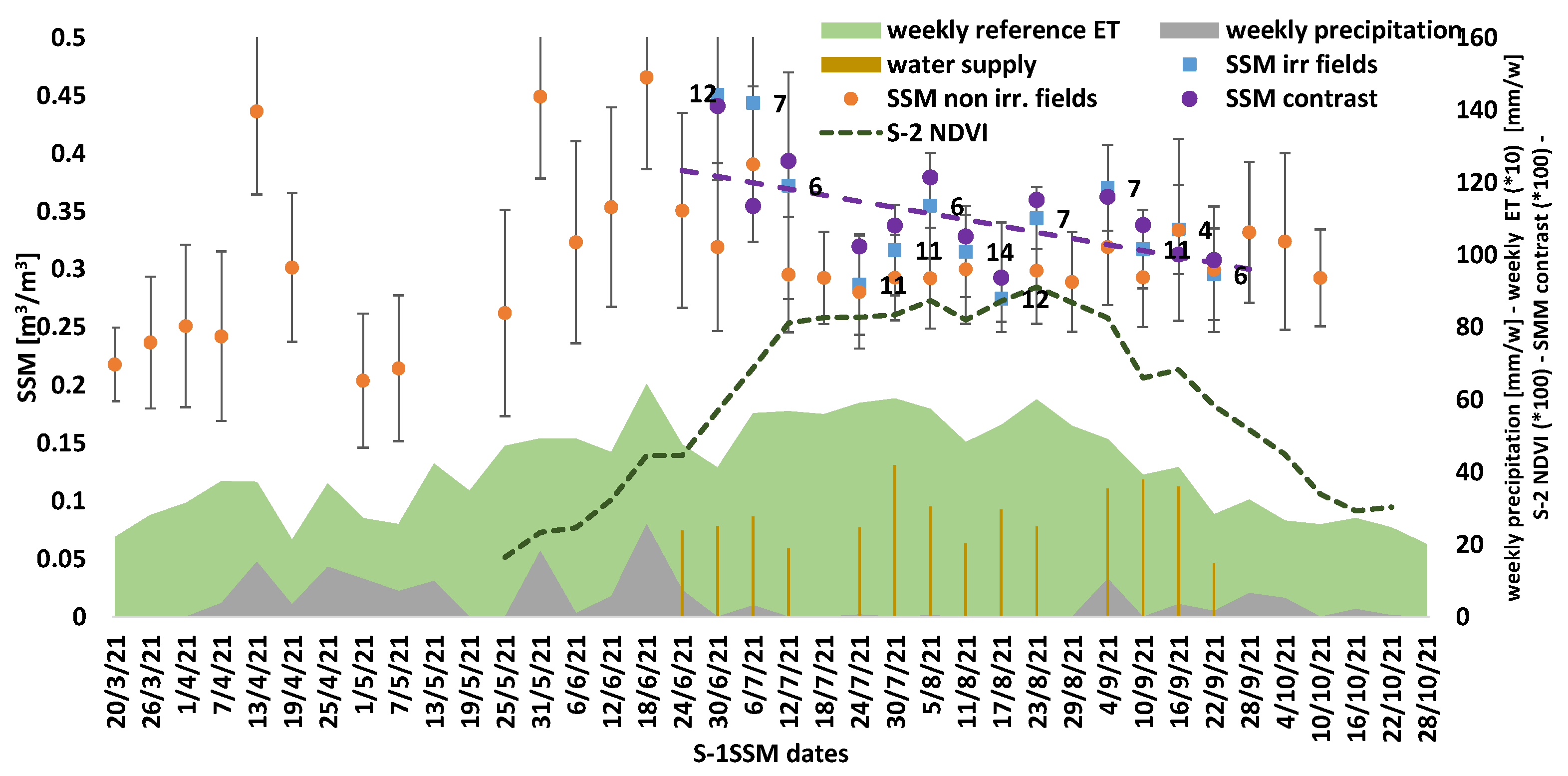
3.1.2. Effect of Precipitation
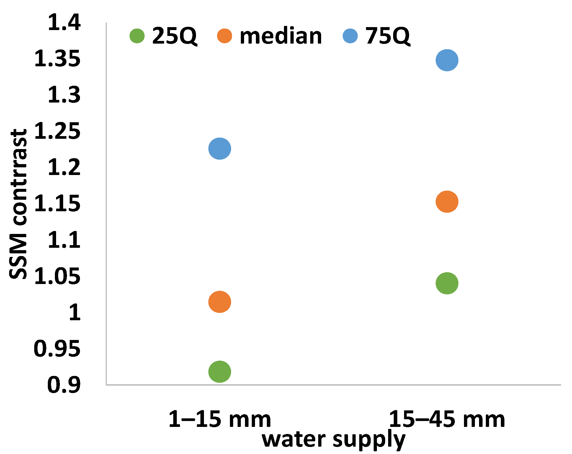
3.1.3. Effect of Water Supply
3.1.4. Effect of Vegetation Cover
3.2. Perspectives for Mapping Irrigated Areas by S-1 and S-2 SSM
4. Conclusions
Author Contributions
Funding
Institutional Review Board Statement
Informed Consent Statement
Data Availability Statement
Acknowledgments
Conflicts of Interest
References
- United Stations Environment Programme. Mediterranean Action Plan. UNEP/MED WG.502/6 2021. Available online: https://www.rac-spa.org/publications (accessed on 26 September 2022).
- Tramblay, Y.; Koutroulis, A.; Samaniego, L.; Vicente-Serrano, S.M.; Volaire, F.; Boone, A.; Le Page, M.; Llasat, M.C.; Albergel, C.; Burak, S.; et al. Challenges for Drought Assessment in the Mediterranean Region under Future Climate Scenarios. Earth-Sci. Rev. 2020, 210, 103348. [Google Scholar] [CrossRef]
- IPCC. Climate Change 2022: Impacts, Adaptation, and Vulnerability. Contribution of Working Group II to the Sixth Assessment Report of the Intergovernmental Panel on Climate Change; Pörtner, H.-O., Roberts, D.C., Tignor, M., Poloczanska, E.S., Mintenbeck, K., Alegría, A., Craig, M., Langsdorf, S., Löschke, S., Möller, V., et al., Eds.; Cambridge University Press: Cambridge, UK; New York, NY, USA, 2022. [Google Scholar] [CrossRef]
- Food and Agriculture Organization (FAO). The State of Food and Agriculture 2020. Overcoming water Challenges in Agriculture; FAO: Rome, Italy, 2020; ISBN 978-92-5-133441-6. [Google Scholar]
- Ferguson, C.R.; Pan, M.; Oki, T. The Effect of Global Warming on Future Water Availability: CMIP5 Synthesis. Water Resour. Res. 2018, 54, 7791–7819. [Google Scholar] [CrossRef]
- Islam, N.; Winkel, J. Climate Change and Social Inequality. DESA Working Paper No. 152, ST/ESA/2017/DWP/152. 2017. Available online: https://www.un.org/development/desa/publications/working-paper/wp152 (accessed on 26 September 2022).
- Rosa, L. Adapting agriculture to climate change via sustainable irrigation: Biophysical potentials and feedbacks. Environ. Res. Lett. 2022, 17, 063008. [Google Scholar] [CrossRef]
- McNally, A.; McCartney, S.; Ruane, A.C.; Mladenova, I.E.; Whitcraft, A.K.; Becker-Reshef, I.; Bolten, J.D.; Peters-Lidard, C.D.; Rosenzweig, C.; Uz, S.S. Hydrologic and Agricultural Earth Observations and Modeling for the Water-Food Nexus. Front. Environ. Sci. 2019, 7, 23. [Google Scholar] [CrossRef]
- Zajac, Z.; Gomez, O.; Gelati, E.; van der Velde, M.; Bassu, S.; Ceglar, A.; Chukaliev, O.; Panarello, L.; Koeble, R.; van den Berg, M.; et al. Estimation of spatial distribution of irrigated crop areas in Europe for large-scale modelling applications. Agric. Water Manag. 2022, 266, 107527. [Google Scholar] [CrossRef]
- Puy, A.; Borgonovo, E.; Lo Piano, S.; Levin, S.A.; Saltelli, A. Irrigated areas drive irrigation water withdrawals. Nat. Commun. 2021, 12, 4525. [Google Scholar] [CrossRef]
- Paredes-Gómez, V.; Gutiérrez, A.; Del Blanco, V.; Nafría, D.A. A Methodological Approach for Irrigation Detection in the Frame of Common Agricultural Policy Checks by Monitoring. Agronomy 2020, 10, 867. [Google Scholar] [CrossRef]
- Meier, J.; Zabel, F.; Mauser, W. A global approach to estimate irrigated areas–a comparison between different data and statistics. Hydrol. Earth Syst Sci. 2018, 22, 1119–1133. [Google Scholar] [CrossRef]
- Puy, A.; Sheikholeslami, R.; Gupta, H.V.; Hall, J.W.; Lankford, B.; Lo Piano, S.; Meier, J.; Pappenberger, F.; Porporato, A.; Vico, G.; et al. The delusive accuracy of global irrigation water withdrawal estimates. Nat. Commun. 2022, 13, 3183. [Google Scholar] [CrossRef]
- Massari, C.; Modanesi, S.; Dari, J.; Gruber, A.; De Lannoy, G.J.M.; Girotto, M.; Quintana-Seguí, P. A review of irrigation information retrievals from space and their utility for users. Remote Sens. 2021, 13, 4112. [Google Scholar] [CrossRef]
- Karthikeyan, L.; Chawla, I.; Mishra, A.K. A review of remote sensing applications in agriculture for food security: Crop growth and yield, irrigation, and crop losses. J. Hydrol. 2020, 586, 124905. [Google Scholar] [CrossRef]
- Ha, W.; Gowda, P.H.; Howell, T.A. A review of downscaling methods for remote sensing-based irrigation management: Part I. Irrig. Sci. 2013, 31, 831–850. [Google Scholar] [CrossRef]
- Ha, W.; Gowda, P.H.; Howell, T.A. A review of potential image fusion methods for remote sensing-based irrigation management: Part II. Irrig. Sci. 2013, 31, 851–869. [Google Scholar] [CrossRef]
- Pervez, M.; Budde, M.; Rowland, J. Mapping irrigated areas in Afghanistan over the past decade using MODIS NDVI. Remote Sens. Environ. 2014, 149, 155–165. [Google Scholar] [CrossRef]
- Ambika, A.K.; Wardlow, B.; Mishra, V. Remotely sensed high resolution irrigated area mapping in India for 2000 to 2015. Sci. Data 2016, 3, 160118. [Google Scholar] [CrossRef]
- Gumma, M.K.; Thenkabail, P.S.; Hideto, F.; Nelson, A.; Dheeravath, V.; Busia, D.; Rala, A. Mapping irrigated areas of Ghana using fusion of 30 m and 250 m resolution remote-sensing data. Remote Sens. 2011, 3, 816–835. [Google Scholar] [CrossRef]
- Xie, Y.; Lark, T.J.; Brown, J.F.; Gibbs, H.K. Mapping irrigated cropland extent across the conterminous United States at 30 m resolution using a semi-automatic training approach on Google Earth Engine. ISPRS J. Photogramm. Remote Sens. 2019, 155, 136–149. [Google Scholar] [CrossRef]
- Lawston, P.M.; Santanello, J.A., Jr.; Kumar, S.V. Irrigation signals detected from SMAP soil moisture retrievals. Geophys. Res. Lett. 2017, 44, 11–860. [Google Scholar] [CrossRef]
- Brocca, L.; Tarpanelli, A.; Filippucci, P.; Dorigo, W.; Zaussinger, F.; Gruber, A.; Fernández-Prieto, D. How much water is used for irrigation? A new approach exploiting coarse resolution satellite soil moisture products. Int. J. Appl. Earth Obs. Geoinf. 2018, 73, 752–766. [Google Scholar] [CrossRef]
- Dari, J.; Quintana-Seguí, P.; Escorihuela, M.J.; Stefan, V.; Brocca, L.; Morbidelli, R. Detecting and mapping irrigated areas in a Mediterranean environment by using remote sensing soil moisture and a land surface model. J. Hydrol. 2021, 596, 126129. [Google Scholar] [CrossRef]
- El Hajj, M.; Baghdadi, N.; Zribi, M.; Bazzi, H. Synergic use of Sentinel-1 and Sentinel-2 images for operational soil moisture mapping at high spatial resolution over agricultural areas. Remote Sens. 2017, 9, 1292. [Google Scholar] [CrossRef]
- Bauer-Marschallinger, B.; Freeman, V.; Cao, S.; Paulik, C.; Schaufler, S.; Stachl, T.; Modanesi, S.; Massari, C.; Ciabatta, L.; Brocca, L.; et al. Toward global soil moisture monitoring with Sentinel-1: Harnessing assets and overcoming obstacles. IEEE Trans. Geosci. Remote Sens. 2018, 57, 520–539. [Google Scholar] [CrossRef]
- Balenzano, A.; Mattia, F.; Satalino, G.; Lovergine, F.P.; Palmisano, D.; Peng, J.; Marzahn, P.; Wegmüller, U.; Cartus, O.; Dąbrowska-Zielińska, K.; et al. Sentinel-1 soil moisture at 1 km resolution: A validation study. Remote Sens. Environ. 2021, 263, 112554. [Google Scholar] [CrossRef]
- Gao, Q.; Zribi, M.; Escorihuela, M.J.; Baghdadi, N.; Segui, P.Q. Irrigation mapping using Sentinel-1 time series at field scale. Remote Sens. 2018, 10, 1495. [Google Scholar] [CrossRef]
- Bousbih, S.; Zribi, M.; El Hajj, M.; Baghdadi, N.; Lili-Chabaane, Z.; Gao, Q.; Fanise, P. Soil moisture and irrigation mapping in A semi-arid region, based on the synergetic use of Sentinel-1 and Sentinel-2 data. Remote Sens. 2018, 10, 1953. [Google Scholar] [CrossRef]
- Elwan, E.; Le Page, M.; Jarlan, L.; Baghdadi, N.; Brocca, L.; Modanesi, S.; Dari, J.; Quintana Seguí, P.; Zribi, M. Irrigation mapping on two contrasted climatic contexts using Sentinel-1 and Sentinel-2 data. Water 2022, 14, 804. [Google Scholar] [CrossRef]
- Dari, J.; Brocca, L.; Quintana-Seguí, P.; Casadei, S.; Escorihuela, M.J.; Stefan, V.; Morbidelli, R. Double-scale analysis on the detectability of irrigation signals from remote sensing soil moisture over an area with complex topography in central Italy. Adv. Water Resour. 2022, 161, 104130. [Google Scholar] [CrossRef]
- Bazzi, H.; Baghdadi, N.; Amin, G.; Fayad, I.; Zribi, M.; Demarez, V.; Belhouchette, H. An Operational Framework for Mapping Irrigated Areas at Plot Scale Using Sentinel-1 and Sentinel-2 Data. Remote Sens. 2021, 13, 2584. [Google Scholar] [CrossRef]
- Ali, E.; Cramer, W.; Carnicer, J.; Georgopoulou, E.; Hilmi, N.J.M.; le Cozannet, G.; Lionello, P. Cross-Chapter Paper 4: Mediterranean Region. In Climate Change 2022: Impacts, Adaptation and Vulnerability. Contribution of Working Group II to the Sixth Assessment Report of the Intergovernmental Panel on Climate Change; Pörtner, H.-O., Roberts, D.C., Tignor, M., Poloczanska, E.S., Mintenbeck, K., Alegría, A., Craig, M., Langsdorf, S., Löschke, S., Möller, V., et al., Eds.; Cambridge University Press: Cambridge, UK; New York, NY, USA, 2022; pp. 2233–2272. [Google Scholar] [CrossRef]
- Ouellette, J.D.; Johnson, J.T.; Balenzano, A.; Mattia, F.; Satalino, G.; Kim, S.B.; Dunbar, R.S.; Colliander, A.; Cosh, M.H.; Caldwell, T.G.; et al. A time-series approach to estimating soil moisture from vegetated surfaces using L-band radar backscatter. IEEE Trans. Geosci. Remote Sens. 2017, 55, 3186–3193. [Google Scholar] [CrossRef]
- Iacobellis, V.; Gioia, A.; Milella, P.; Satalino, G.; Balenzano, A.; Mattia, F. Inter-comparison of hydrological model simulations with time series of SAR-derived soil moisture maps. Eur. J. Remote Sens. 2013, 46, 739–757. [Google Scholar] [CrossRef]
- Satalino, G.; Balenzano, A.; Mattia, F.; Davidson, M.W.J. C-band SAR data for mapping crops dominated by surface or volume scattering. IEEE Geosci. Remote Sens. Lett. 2014, 11, 384–388. [Google Scholar] [CrossRef]
- Palmisano, D.; Mattia, F.; Balenzano, A.; Satalino, G.; Pierdicca, N.; Guarnieri, A.V.M. Sentinel-1 sensitivity to soil moisture at high incidence angle and the impact on retrieval over seasonal crops. IEEE Trans. Geosci. Remote Sens. 2021, 59, 7308–7321. [Google Scholar] [CrossRef]
- Quegan, S.; Yu, J.J. Filtering of multichannel SAR images. IEEE Trans. Geosci. Remote Sens. 2001, 39, 2373–2379. [Google Scholar] [CrossRef]
- Sentinel-2 MSI User Guide Product Type: Level-2A. April 2019. Available online: https://sentinel.esa.int/web/sentinel/user-guides/sentinel-2-msi/product-types/level-2a (accessed on 26 September 2022).
- Mattia, F.; Balenzano, A.; Satalino, G.; Lovergine, F.; Peng, J.; Wegmuller, U.; Cartus, O.; Davidson, M.W.J.; Kim, S.; Johnson, J.; et al. Sentinel-1 & Sentinel-2 for SOIL Moisture Retrieval at Field Scale. In Proceedings of the IGARSS 2018—2018 IEEE International Geoscience and Remote Sensing Symposium, Valencia, Spain, 22–27 July 2018; pp. 6143–6146. [Google Scholar] [CrossRef]
- Mattia, F.; Satalino, G.; Balenzano, A.; Lovergine, F.P.; D’Addabbo, A. Final SSM Algorithm Theoretical Basis Document. EU SARAGRI Project, Deliverable 3.8. 2019. Available online: https://leoipl.uv.es/sensagri/ftp/DELIVERABLES/WP3/SENSAGRI_D3_8_v10.pdf (accessed on 26 September 2022).
- Paredes Gómez, V.; Balenzano, A.; Mattia, F.; Satalino, G.; Lovergine, F.P.; D’Addabbo, A.; Nafría García, D. Second Validation of Surface Soil Moisture Maps. EU SARAGRI Project, Deliverable 7.16. 2019. Available online: https://leoipl.uv.es/sensagri/ftp/DELIVERABLES/WP7/SENSAGRI_D7.16_v10.pdf (accessed on 26 September 2022).
- Balenzano, A.; Mattia, F.; Satalino, G.; Davidson, M. Dense temporal series of C-and L-band SAR data for soil moisture retrieval over agricultural crops. IEEE J. Sel. Top. Appl. Earth Obs. Remote Sens. 2011, 4, 439–450. [Google Scholar] [CrossRef]
- Product User Guide. 2017. ESA Land Cover CCI v2.0. Tech. Rep. Available online: https://www.esa-landcover-cci.org/?q=node/199 (accessed on 26 September 2022).
- Mattia, F. Coherent and incoherent scattering from tilled soil surfaces. Waves Random Complex Media 2011, 21, 278–300. [Google Scholar] [CrossRef]
- Mattia, F.; Le Toan, T.; Davidson, M. An analytical, numerical, and experimental study of backscattering from multiscale soil surfaces. Radio Sci. 2001, 36, 119–135. [Google Scholar] [CrossRef]
- Famiglietti, J.S.; Ryu, D.; Berg, A.A.; Rodell, M.; Jackson, T.J. Field observations of soil moisture variability across scales. Water Resour. Res. 2008, 44, W01423. [Google Scholar] [CrossRef] [Green Version]
- Rysman, J.F.; Verrier, S.; Lemaître, Y.; Moreau, E. Space-time variability of the rainfall over the western Mediterranean region: A statistical analysis. J. Geophys. Res. Atmos. 2013, 118, 8448–8459. [Google Scholar] [CrossRef]
- Chiaravalloti, F.; Brocca, L.; Procopio, A.; Massari, C.; Gabriele, S. Assessment of GPM and SM2RAIN-ASCAT rainfall products over complex terrain in southern Italy. Atmos. Res. 2018, 206, 64–74. [Google Scholar] [CrossRef]
- Le Page, M.; Jarlan, L.; El Hajj, M.M.; Zribi, M.; Baghdadi, N.; Boone, A. Potential for the Detection of Irrigation Events on Maize Plots Using Sentinel-1 Soil Moisture Products. Remote Sens. 2020, 12, 1621. [Google Scholar] [CrossRef]
- Bazzi, H.; Baghdadi, N.; Fayad, I.; Charron, F.; Zribi, M.; Belhouchette, H. Irrigation Events Detection over Intensively Irrigated Grassland Plots Using Sentinel-1 Data. Remote Sens. 2020, 12, 4058. [Google Scholar] [CrossRef]
- Davidson, M.; Iannini, L.; Torres, R.; Geudtner, D. New perspectives for applications and services provided by future spaceborne SAR missions at the European Space Agency. In Proceedings of the International Geoscience and Remote Sensing Symposium (IGARSS2022), Kuala Lumpur, Malaysia, 17–22 July 2022; pp. 4720–4723. [Google Scholar]
- Bazzi, H.; Baghdadi, N.; Charron, F.; Zribi, M. Comparative Analysis of the Sensitivity of SAR Data in C and L Bands for the Detection of Irrigation Events. Remote Sens. 2022, 14, 2312. [Google Scholar] [CrossRef]


Publisher’s Note: MDPI stays neutral with regard to jurisdictional claims in published maps and institutional affiliations. |
© 2022 by the authors. Licensee MDPI, Basel, Switzerland. This article is an open access article distributed under the terms and conditions of the Creative Commons Attribution (CC BY) license (https://creativecommons.org/licenses/by/4.0/).
Share and Cite
Balenzano, A.; Satalino, G.; Lovergine, F.P.; D’Addabbo, A.; Palmisano, D.; Grassi, R.; Ozalp, O.; Mattia, F.; Nafría García, D.; Paredes Gómez, V. Sentinel-1 and Sentinel-2 Data to Detect Irrigation Events: Riaza Irrigation District (Spain) Case Study. Water 2022, 14, 3046. https://doi.org/10.3390/w14193046
Balenzano A, Satalino G, Lovergine FP, D’Addabbo A, Palmisano D, Grassi R, Ozalp O, Mattia F, Nafría García D, Paredes Gómez V. Sentinel-1 and Sentinel-2 Data to Detect Irrigation Events: Riaza Irrigation District (Spain) Case Study. Water. 2022; 14(19):3046. https://doi.org/10.3390/w14193046
Chicago/Turabian StyleBalenzano, Anna, Giuseppe Satalino, Francesco Paolo Lovergine, Annarita D’Addabbo, Davide Palmisano, Riccardo Grassi, Ozlem Ozalp, Francesco Mattia, David Nafría García, and Vanessa Paredes Gómez. 2022. "Sentinel-1 and Sentinel-2 Data to Detect Irrigation Events: Riaza Irrigation District (Spain) Case Study" Water 14, no. 19: 3046. https://doi.org/10.3390/w14193046