
Two-Step Simulation of Underwater Terrain in River Channel
1
Department of Naval Architecture and Ocean Engineering, Jiangsu Maritime Institute, Nanjing 211170, China
2
Nanjing Water Planning and Design Institute Co., Ltd., Nanjing 210022, China
3
Key Laboratory of Virtual Geographic Environment, Ministry of Education, Nanjing Normal University, Nanjing 210023, China
4
School of Resources and Geosciences, China University of Mining Technology, Xuzhou 221000, China
*
Authors to whom correspondence should be addressed.
Water 2022, 14(19), 3041; https://doi.org/10.3390/w14193041
Submission received: 23 August 2022
/
Revised: 14 September 2022
/
Accepted: 19 September 2022
/
Published: 27 September 2022
(This article belongs to the Section Hydrology)
Abstract
:When studying river hydrodynamics and water quality evolution laws on the basis of numerical simulation analysis, it is necessary to carry out topographic interpolation along the bend direction of the river on the basis of the measured river section, as this can provide accurate and reliable topographic data for river numerical modeling. In this paper, a two-step terrain simulation method based on sparse and discrete river sections is proposed by comprehensively considering the river trends and the lack of monitoring sections. On the basis of establishing a reference using the river centerline and coding the spatial relationship of the river, the linear weight method, which uses the distance and gradient change between the known sampling elevation section to realize the preliminary encryption of spatial points with any number of longitudinal sections and any horizontal distance, is carried out first. Considering the structural and anisotropic characteristics of the river, the improved inverse distance weighting (IDW) method is further used to locally interpolate the encrypted points to obtain the continuous surface of the river terrain. In order to prove the effectiveness of this method, a part of the Qinhuai River in Nanjing was taken as the research object. The experiment was carried out by setting different spacing distances for preliminary densification and by using different interpolation methods for further local terrain simulation. Root mean square error (RMSE) and mean absolute error (MAE) are used to evaluate the overall performance of different simulation methods. The experimental results show that the method proposed in this paper overcomes the obvious inaccuracy of directly using an interpolation algorithm to generate the river terrain due to sparse section data. The river terrain generated by the preliminary densification and improved IDW interpolation calculation method is more reasonable, and continuous and unobstructed, reflecting the original river terrain more accurately.
1. Introduction
With the development of the economy and increased urbanization, environmental problems related to surface water are becoming more prominent, especially in surface water bodies such as urban rivers and lakes, which are becoming seriously polluted [1]. In order to study the changes in surface water environments, many scholars established numerical models to analyze the changes in surface water dynamics and water quality [2,3,4,5,6,7]. Terrain simulation is an important part of the numerical simulations of surface water. The quality of underwater terrain simulations directly affects the accuracy and reliability of simulation results.
Underwater terrain simulations generally use existing elevation sample data and adopt spatial interpolation technology to generate riverbed terrains that meet the application requirements. This is an important river management problem that needs to be solved. Some scholars have carried out relevant research on underwater terrain simulation. Ren Yong and others intervened and optimized the irregular triangulation network of the Jinsha River channel to manually generate contour lines quickly, reasonably, and accurately [8]. Hou Mingrui introduced the cellular method into the terrain reconstruction process. By simplifying the complex river dynamics process, he established a terrain reconstruction model on the basis of the cellular method that was better able to avoid the unnatural strip terrain generated by the terrain structure [9]. Using SMS software, Chen Zhong proposed an interpolation technology based on a triangular mesh [10]. Marcelo used a variety of spatial interpolation methods to generate a water depth map of the Amazon reservoir to optimize the operation and management of the reservoir [11]. Amante used IDW, spline, triangular irregular networks (TINs), and other methods to perform spatial interpolation on Kachemak Bay, and analyzed the influence of the parameters of the spatial interpolation method on the simulation accuracy [12]. Kang used the Australian National University digital elevation model (ANUDEM) method to carry out the spatial interpolation of tidal flat terrain and verified it by combining it with the simulation results of a hydrological model [13]. Zhang defined the time that water spends flowing between two places to represent the Euclidean distance during spatial interpolation and found that it could effectively improve simulation accuracy [14]. Legleiter decomposed a riverbed terrain into trend and residual components, and used the improved Kriging method for spatial interpolation research [15]. Wu used the terrain simulation method by considering anisotropy to simulate the riverbed terrain of the lower Mississippi River [16].
However, many studies mainly focused on the accuracy of the spatial interpolation algorithm itself, ignoring the spatial relationships between the original samples, such as those between the distribution and density [17,18]. The accuracy of spatial interpolation largely depends on the distribution and density of the elevation sampling points [19]. Due to the limitations caused by humans, materials, and financial and technical conditions, it is impossible to measure the full coverage of surface water bodies such as rivers and lakes [20]. For river channels in particular, in many practical cases, there are no continuous topographic data of the whole river channel. During actual operation, only a certain number of elevation sampling section data can be obtained, and these data reflect the local or partial characteristics of the terrain. During numerical simulation, it is necessary to obtain continuous distribution data such as grid surface terrain values from limited and discrete section data through certain methods, especially in places with large fluctuations, such as river bends or river intersections [21]. However, only relying on the original elevation’s sampling data for direct interpolation often leads to the problem of abnormal terrain. Considering the trend of the interpolated river and the insufficient factors of the monitoring section, how to carry out high-precision refinement and further precise interpolation on the basis of limited sampling data is the key to terrain simulation.
To establish a model that is consistent with the process and spatial variation of geographical phenomena, spatial interpolation must consider the spatial structure and anisotropy of geographical phenomena [22,23]. A spatial structure refers to the relationship between the similarity of the attributes of geographical phenomena and the distance between geographical phenomena in space. The closer the distance is, the higher the similarity of the attributes between geographical phenomena. At the same time, under the influence of various factors, the attributes of geographical phenomena show different speeds in different directions [24].
In general, underwater river bottom terrain elevation tends to change uniformly as the longitudinal stake position of the river changes, and the river cross-section tends to be V- or U-shaped, rendering it nonlinear [25]. A two-step terrain simulation method based on a sparse and discrete river section is proposed by comprehensively considering the river trend and the lack of monitoring section. Using the linear weight method, the preliminary densified points with any number of longitudinal sections and any horizontal distance are obtained to control the river terrain as a whole. This can better reflect the longitudinal trend of the river with the flow direction. Further, the original sampling points and encrypted points are locally interpolated by improved IDW interpolation to obtain the continuous surface of the river terrain. This not only ensures the structure of the terrain in the longitudinal direction of the river, but also takes into account the local anisotropy in the direction of the river section to avoid the problem of generating abnormal terrain due to sparse terrain section data.
2. Methods
2.1. Data Preprocessing
2.1.1. Spatial Reference Positioning
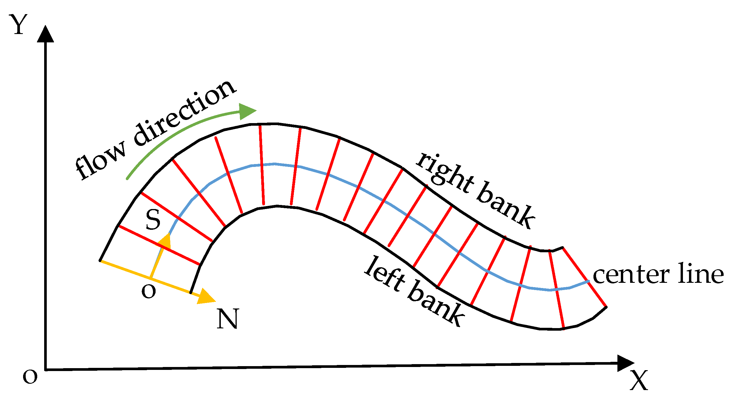
As the meandering, curvature, and flow directions change, the topographic characteristics of the river often create challenges when analyzing river data. For example, most geographic information system (GIS) software packages with interpolation tools are only applicable to Cartesian coordinates (x, y), resulting in much inconvenience when judging the spatial data on the left and right banks, and upstream and downstream of the river. Therefore, taking the river center line as the spatial reference is a necessary procedure for data preprocessing. The reference system is the S axis, which runs along the flow direction; the N axis runs across the flow direction and is perpendicular to the S axis [26]. Previous studies introduced GIS programs or mathematical algorithms that use “straightening” programs to convert regular Cartesian (x, y) systems into channel-centered (s, n) coordinate systems. This paper draws on the spatial reference location method designed by Merwade. The upstream and downstream relationship of the section is judged by the S axis, and the left and right banks of the spatial point are judged by the N axis. The starting point of S is the upstream source of the river. Looking upstream along the S axis, the left bank is on the left, and the right bank is on the right. The spatial reference is shown in Figure 1.
2.1.2. Spatial Element Coding
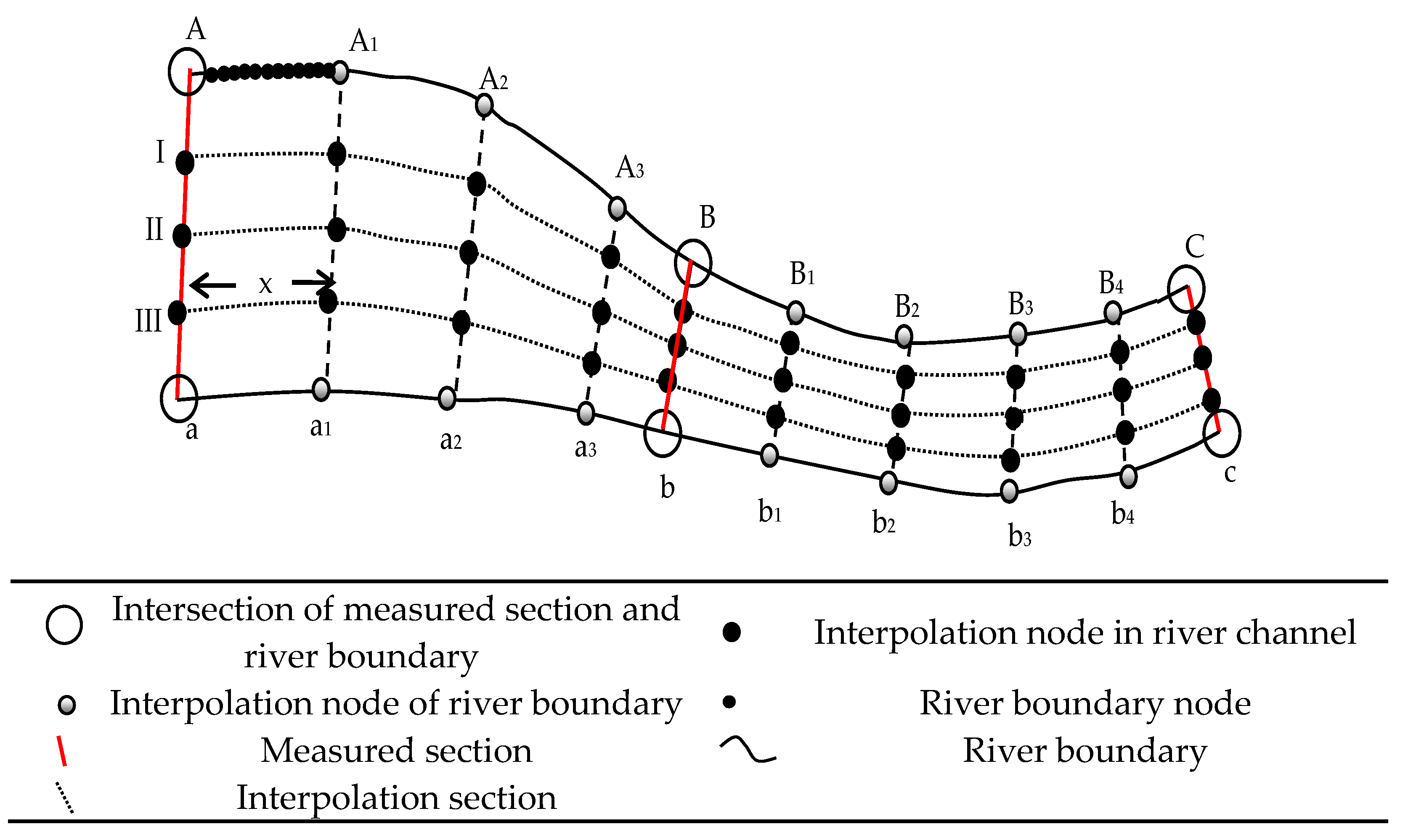
First, the intersection node is determined between the measured section, and river boundaries A, a, B, b, as shown in Figure 2. The node’s coordinate position (such as A1, A2, and A3 in Figure 2) on the boundary of the interpolated section is calculated according to the boundary node of the adjacent section and the longitudinal spacing distance (such as x in Figure 2) or the equal proportion of the interpolated section. The following method was used for node coding and identification: ArcGIS was used to take nodes at equal intervals between the left and right bank boundaries of the river (spacing set to 1 m) and to code each node. Through node traversal, the node closest to the measured section was identified. This node was very close to the intersection and was in the approximate location of the intersection. The boundary file included two node coordinate files on the left and right banks. The measured points on the section needed to be compiled according to the rules from upstream to downstream and from the left bank to the right bank. As shown in Figure 2, the left and right banks of the river were A, B, and C; and a, b, and c, respectively. The measured sections were A–A, B–B, and C–C. The new interpolated transverse sections were A1, A2, A2, etc. The new interpolated longitudinal sections were I, II, and III.
2.2. Global Linear Control
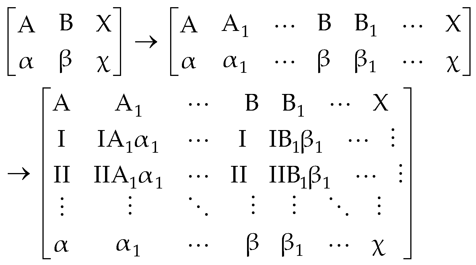
The interpolation section includes the calculation of the node coordinates of the transverse and longitudinal sections. According to the section nodes determined on the left and right bank boundaries of the river, and the interpolation section spacing set, the interpolation node code of the transverse section was determined, and the node coordinates were calculated. The equidistant longitudinal section nodes were determined according to the nodes at both ends of each cross section. The expansion method is shown in Figure 3.
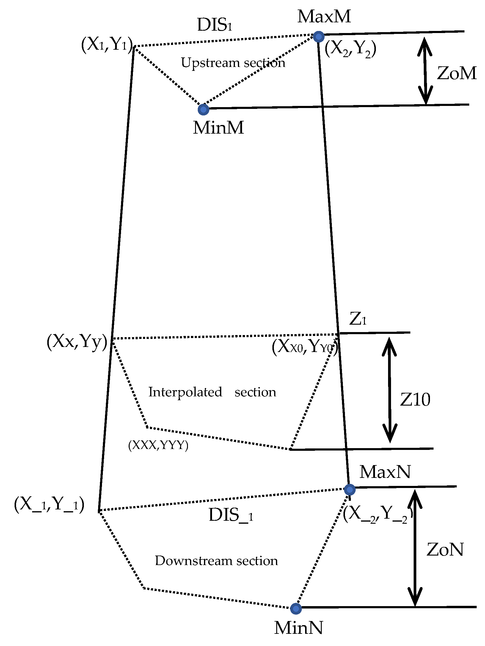
The calculation of the horizontal position and the elevation of the interpolation node is shown in Figure 4, which mainly follows the principles of proportion, continuity, and proximity. According to the starting- and end-point coordinates on the left and right bank boundaries of the upstream and downstream sections, and the position proportions of the interpolated section between the upstream and downstream sections, the starting- and end-point coordinates on the left and right bank boundaries of the interpolated section can be obtained. Assuming that the river bottom terrain model is relatively stable, terrain undulations were relatively continuous (without cliff mutation), and the river bottom terrain elevation showed a uniform change trend with the change in the pile position. If the interpolated section were close to the upstream section, then the section shape was more similar to the upstream section; on the other hand, the shape of the interpolated section was more similar to that of the downstream section.
- (1)
- Calculation of horizontal positions of interpolation nodes
According to the coordinates (X1, Y1), (X_1,Y_1), (X2, Y2), and (X_2, Y_2) of the left and right bank nodes along the upstream and downstream sections that were measured, and the position ratio RAT of the interpolated section between the upstream and downstream sections, the coordinates (XX, YY), (XX0, YY0) of the left and right bank nodes of the interpolated section could be obtained. The calculation formula is as follows:
According to the coordinates of the nodes of the measured upstream and downstream sections, assuming that KK is the slope of the interpolated section in the horizontal direction, and DIS0 is the node spacing of the known upstream or downstream section, it can be obtained by scaling according to the RAT0 ratio of the interpolated section and the measured section width. The basic calculation formula of the horizontal coordinates (XXX, YYY) of other nodes within the interpolated section is as follows:
- (2)
- Calculation of elevation of interpolation node
The highest points MaxM and MaxN, lowest points MinM and MinN, and height differences ZoM and ZoN of the upstream and downstream section nodes were first obtained. Second, the elevation Z1 of the highest point and height difference Z10 between the highest and lowest points were obtained according to the position ratio RAT of the upstream and downstream sections where the interpolation section was located. Lastly, the elevation Z_1 of the interpolation node was obtained by subtracting the height difference Z10 of the scaled corresponding vertices of the upstream or downstream sections from the elevation Z1 of the highest point of the interpolation section. ZM is the vertex elevation of the known upstream (downstream) section. The calculation formula is as follows:
- (a)
- Maximal upstream elevation difference:
ZoM = MaxM − MinM
- (b)
- Maximal downstream elevation difference:
ZoN = MaxN − MinN
- (c)
- Interpolation section height difference:
Z10 = ZoM + RAT* (ZoN − ZoM)
- (d)
- Elevation of the highest point of interpolation section:
Z1 = MaxM + RAT* (MaxN − MaxM)
- (e)
- Elevation of the interpolation node:
Z_1 = Z1 − Z10/ZoN* (MaxN − ZM)
2.3. Local Quadratic Interpolation
There are differences (anisotropy) in the speed of attribute changes in different directions of the space field. When choosing an interpolation method for local interpolation, we need to consider the influence of the anisotropy of the sampling points on the estimation of unknown points [27]. In the current interpolation methods, the IDW method takes the weighted average value of a certain number of sample points within a certain range or that which is the closest to the value of the points to be interpolated, and the required weight is determined according to the distance. The closer the sample points are to the interpolation points, the greater the weight is [28]. The spline method establishes a smooth surface that minimizes the curvature changes of all of the points through the sample points and the points to be interpolated to minimize the total curvature of the surface and to interpolate the points to be interpolated. The Kriging interpolation method regards the spatial field as a random field. After considering the shape, size, and spatial orientation of the sample points, the spatial relationship with the unknown sample points, and the construction information provided by the variogram, a linear unbiased optimal estimation of the unknown sample points is carried out.
Among the many interpolation methods, IDW interpolation is a standard spatial interpolation method in the field of GIS that has been widely used in various disciplines because of its simple principle, simple calculation, and compliance with the first law of geography [29]. In consideration of the influence of anisotropy, an “ellipse” distance was proposed in [30,31,32] to deal with the interpolation problem of anisotropy. It introduces physical distance and direction adjustment parameters to reflect the anisotropy of geographical phenomena and extends the typical Euclidean distance to the “ellipse” distance of each direction.
The IDW interpolation model is shown in Formula (8):
where represents any point to be interpolated; is the measured value at point ; is the distance between unknown point and known point ; is the nearest point; and α is the distance attenuation coefficient.
The value of is determined by several parameters, such as the nearest number of points, the distance between the sample point and the unknown point, and the distance attenuation coefficient. The classical IDW interpolation algorithm uses isotropy to describe the spatial proximity, ignoring the anisotropy that exists in reality. Distance adjustment parameters λ are introduced, and the Euclidean distance is expanded to the “ellipse” distance, as shown in Formula (9).
where and represent the Cartesian coordinates of points and .
From Equation (2), when λ is equal to 1, is equivalent to the Euclidean space distance; when λ > 1, the larger the y between two points is, the farther the distance between the two points in the Y direction; that is, the spatial proximity in the Y direction is weakened. Conversely, when λ < 1, the distance in the X direction between the two points is relatively increased. That is, the spatial proximity in the X direction of the two points is weakened.
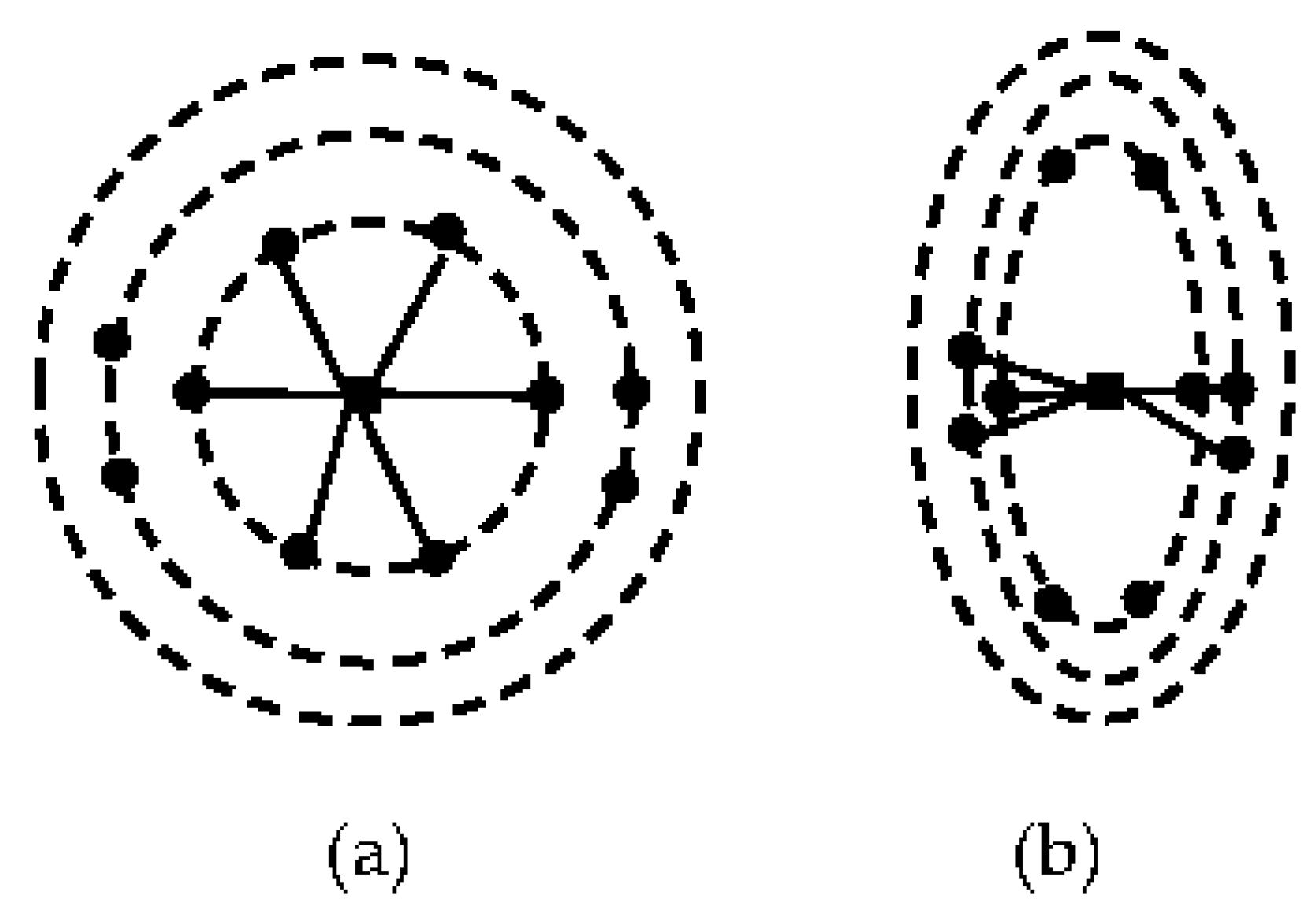
As shown in Figure 5, the distance adjustment parameter can change the nearest neighbor point. Figure 5a shows the spatial neighbor point selected in the homogeneous space, and Figure 5b shows the spatial neighbor point selected when considering anisotropy.
The formula implies that the anisotropy direction of the data is just along the coordinate axis of the data, which is inconsistent with most actual situations. Therefore, direction parameter θ needs to be further introduced to describe anisotropy in the general case so that the conversion relationship between the original coordinates and the coordinates reflecting the anisotropy can be established, as shown in Formula (10).
Formula (11) can be obtained by combining Formulas (9) and (10).
where represents the distance between the point to be interpolated and the sample point in consideration of anisotropy; λ is used to adjust the distance between the different coordinate axes under the coordinate system; represents the rotation angle between the original coordinates and the anisotropic coordinate system; ΔX and ΔY are the Euclidean distance between the point to be interpolated and the known sample point in the original data.
2.4. Verification of Simulated Terrain
Cross-validation methods are some of the most extensive validation methods, and the ‘leave-one-out’ technique is an example of one such method. This method involves omitting a single sample value from the entire dataset and performs the interpolation procedure using the remaining dataset. After the interpolation process, the difference between the actual and predicted values of the omitted point is calculated. This procedure is repeated n times, where n is equal to the number of all samples. ‘Leave one-out’ cross-validation is embedded in the ArcGIS Geostatistical Analyst extension, which provides exploratory analytical results. Several statistical measurements are widely used to evaluate the overall performance of interpolation methods, including the performance of RMSE, MAE, and the bias and coefficient of determination [11]. In this paper, RMSE and MAE are used to evaluate the final terrain simulation results. The following mathematical equations show how to calculate these two statistical measurements.
3. Results and Discussion
In order to test the effectiveness of this method, a part of Qinhuai River in the city of Nanjing was selected as the research object. According to the topographic data measured for the selected cross section of the river, the topographic surface was generated along the bend direction of the river. Because this paper uses a two-step method to generate terrain data, the first step is to use the linear weight method to generate encrypted points from the original sampling data, and the second step uses the local interpolation method to generate continuous surfaces for encrypted points, meaning that the accuracy of both encrypted points and 3D surfaces needs to be verified.
3.1. Study Data
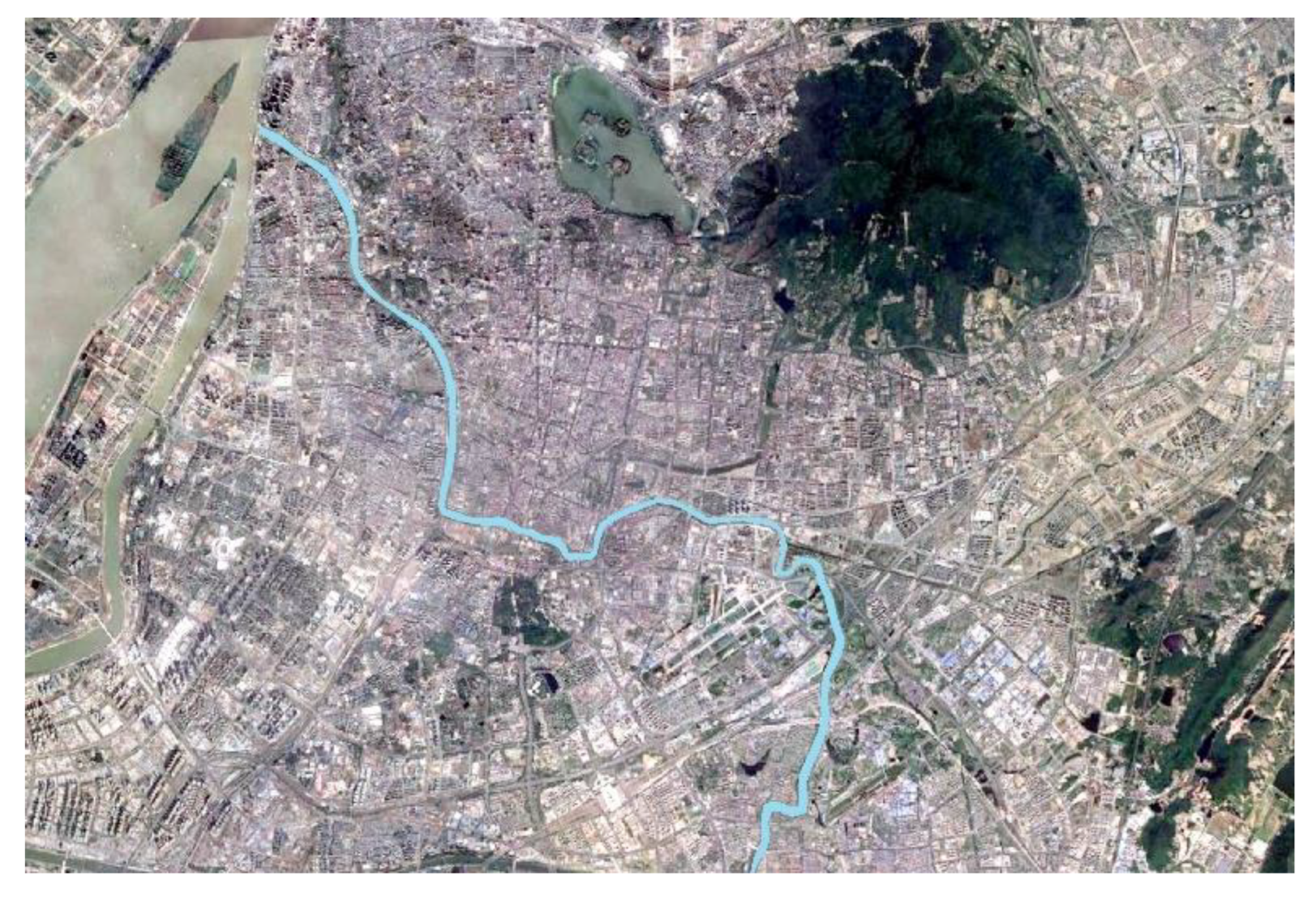
Qinhuai River (Figure 6) is located at 31°35′–32°07′ N and 118°43′–119°18′ E. It is a branch river on the south bank of the lower reaches of the Yangtze River. There is a sluice at Wuding gate, and the average flow, as monitored for many years, is 15 cubic meters per second. In order to study the impact of sewage discharge from the riverside sewage treatment plant on the water quality of the downstream monitoring section, it is proposed that a two-dimensional hydrodynamic water quality model be established for prediction. The spatial data in this experiment adopted the three-degree Gauss Kruger projection with a central longitude of 120 degrees, and the original positioning frame was the CGCS2000 coordinate system.
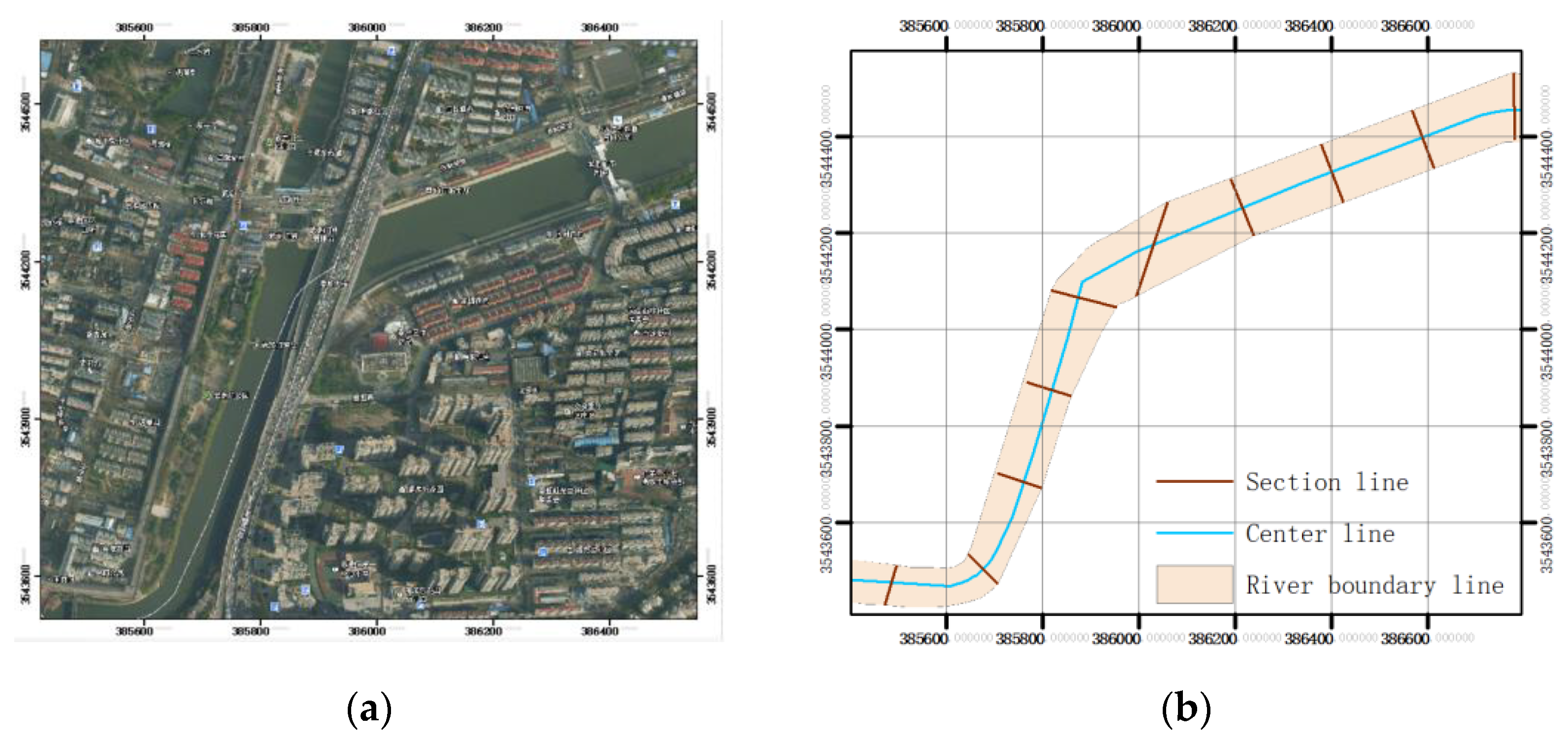
In this example, 10 groups of measurement sections were selected, and about 20 groups of elevation points were measured at equal intervals for each section, resulting in the inclusion of more than 200 measuring points. This part of river is about 1800 m long and 80–120 m wide, and the section position is shown in Figure 7.
3.2. Steps for 3D Surface Generation of River Terrain
The measured data were preprocessed using ArcGIS 10.2 developed by ESRI (Environment System Research Institute) of the United States joint c# programming language published by Microsoft. First, the SHP format files of the river boundary and centerline were obtained by vectoring the left and right banks of the river from the map, and calculating the river centerline, as shown in Figure 7b. Then, according to the spatial reference positioning method in Section 2.1.1 and the spatial element coding method in Section 2.1.2, the measured points on the section were compiled according to the rules from upstream to downstream and from the left bank to the right bank. The intersection of the measured cross-section and the bank boundary was obtained, which was the nearest node coordinate between the measured river cross-section and the river node.
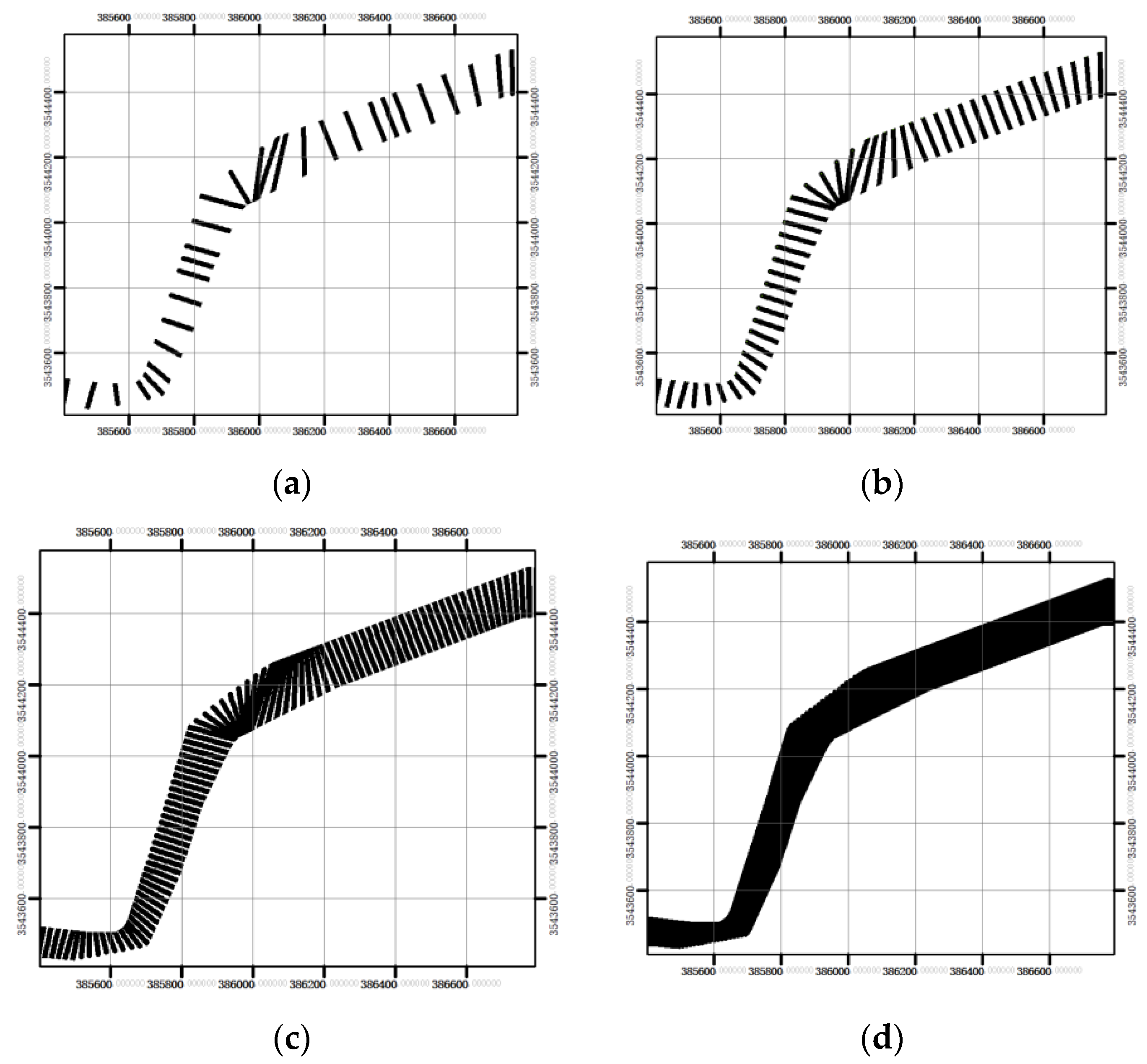
According to the two-step method, the topographic data of six measured sections were initially encrypted. In order to compare the interpolation effects of different densities, the interpolation intervals of the transverse sections were set to 80, 40, 20, and 10 m. The equidistant interpolation nodes of the river boundary between two adjacent measured sections can be calculated to determine section lines A1, a1, etc. The number of longitudinal sections was set to n = 5, and the corresponding equidistant nodes were calculated, which were in the river channel along the interpolated section line. After the horizontal position of the preliminary densification point had been calculated, according to the river bottom elevation of the measured section, the overall linear weight method proposed in Article 2.2 was used to calculate the river bottom elevation value of the node in the river between two adjacent measured sections, and multiple groups of river bottom elevations were obtained (Figure 8).
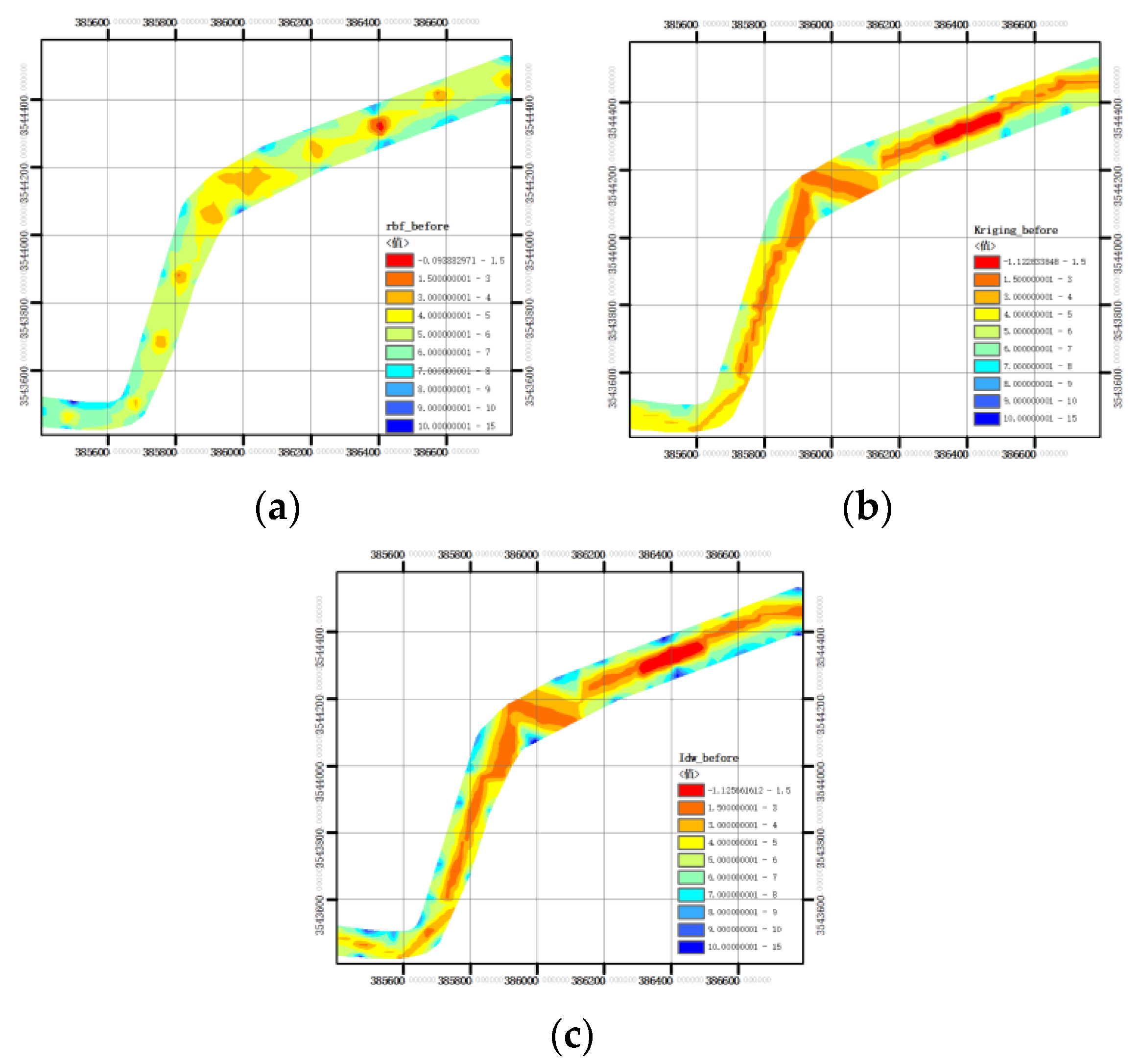
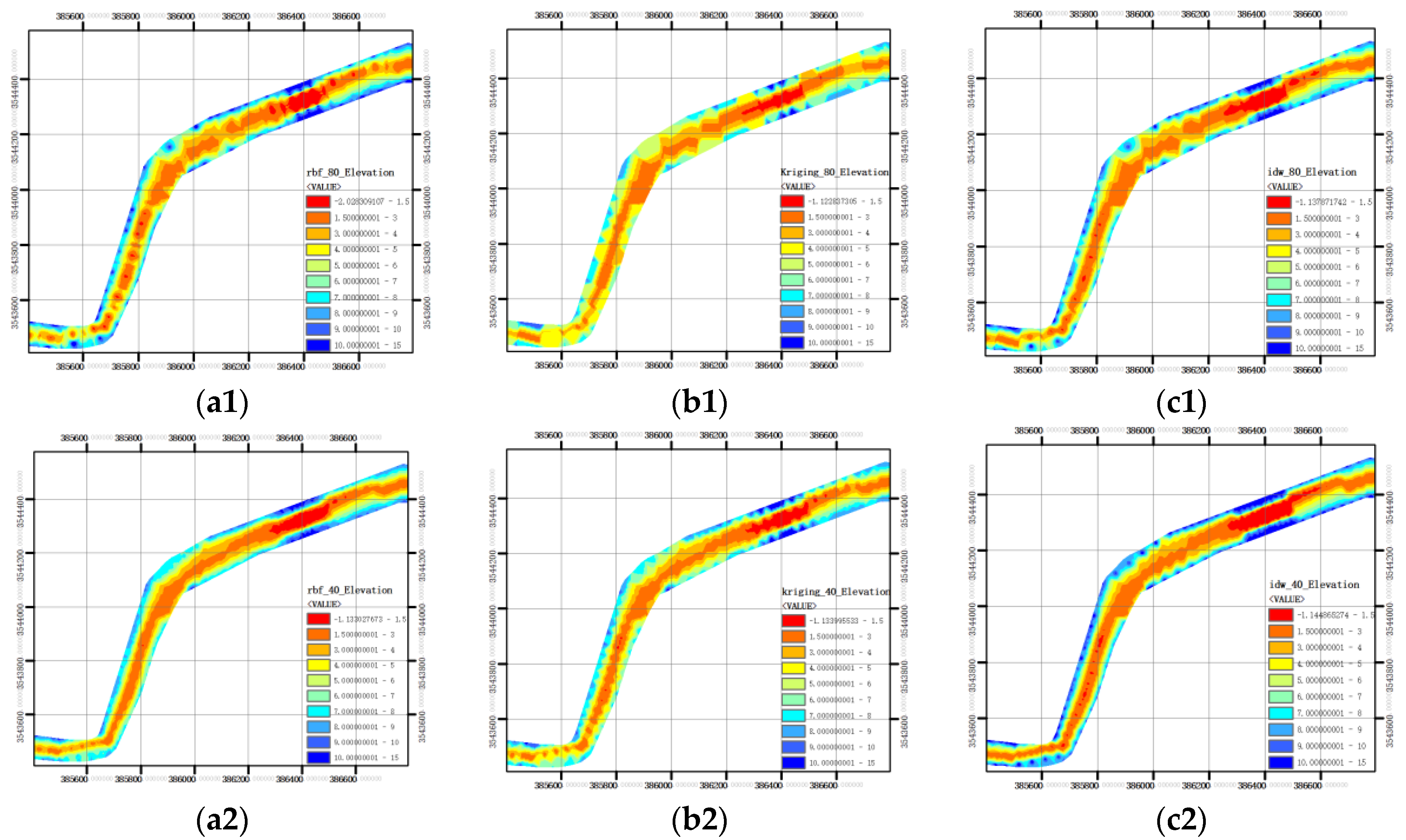
In this paper, in order to verify the influence of preliminary encryption on the final terrain simulation and the effect of different local interpolation methods, on the basis of obtained data before and after the encryption of sampling points, the river channel terrain in the study area was simulated using the improved IDW method, the local RBF method, and the ordinary Kriging method. Figure 9 and Figure 10 show the simulation results in the CGCS2000 coordinate system. The color in the result graph represents the elevation interval. Figure 9 shows that, when the original sampling points were directly interpolated and simulated with RBF, Kriging, or IDW, the results were not ideal, which was obviously different from the actual terrain. According to the two-step method in this paper, when the original sampling points were encrypted first and then interpolated by RBF, Kriging, or IDW, the final simulation results were closer to the actual terrain, as the encryption interval was gradually reduced from 80 to 10 m, as shown in Figure 10.
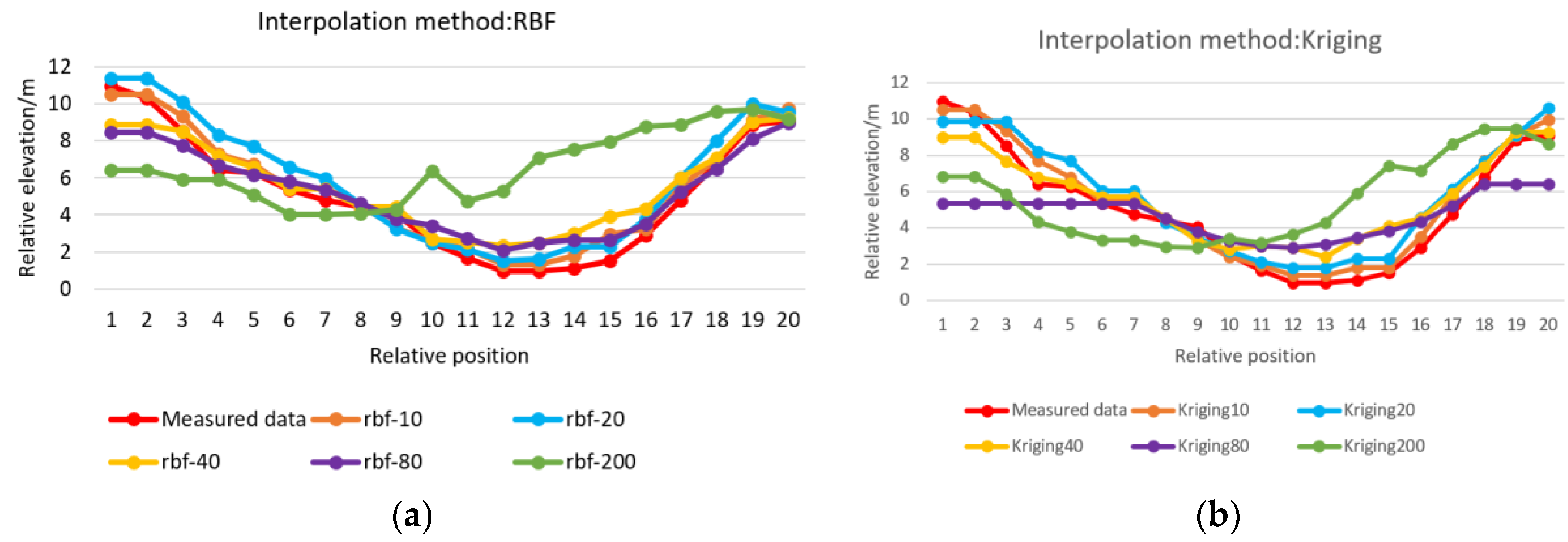
In order to more intuitively observe the impact of the encryption interval on the simulation results, as shown in Figure 11, any section could be randomly selected for observation. By comparing the measured values of 20 sampling points on the section and the calculation results of further interpolation under the different encryption intervals, no matter which interpolation method was used during the later stages, the smaller the encryption interval in the earlier stage was, the closer the final simulation result was to the actual terrain. If RBF, Kriging, or IDW were directly used to interpolate the sampled point data without initial encryption processing, the simulated elevation error value could be up to 5 m or even more.
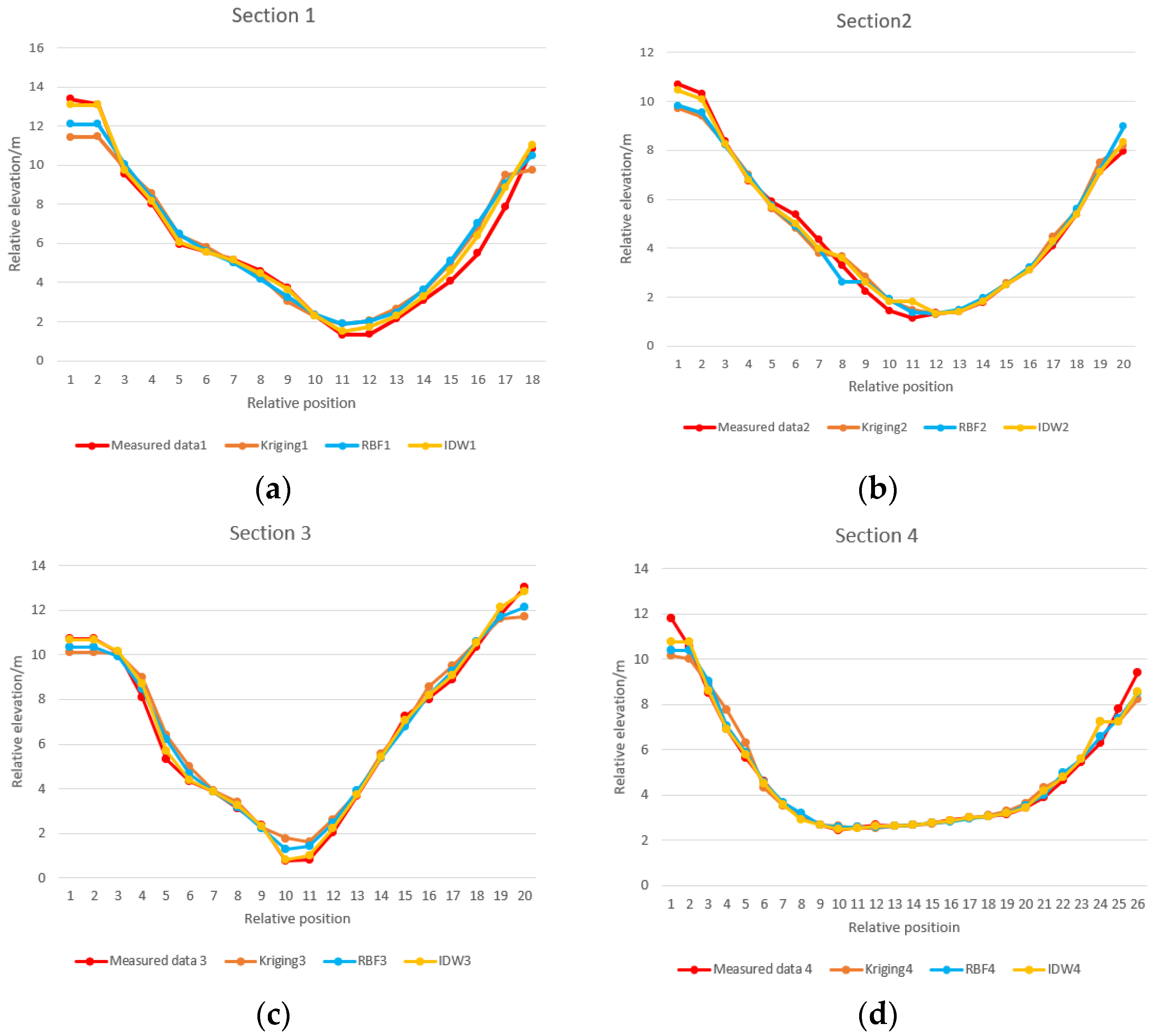
In this paper, four groups of measured section data (as shown in Figure 12, Sections 1–4) were used to analyze and test the influence of different local interpolation methods on the accuracy of the generated river terrain when the section spacing is 10 m. Figure 12 shows that the simulation results using the IDW interpolation method were better than those obtained when using RBF and Kriging for the four sections.
In order to more objectively analyze the simulation effects of the different interpolation methods and different intervals, RMSE and MAE were taken as the evaluation indices of the final terrain simulation, and the results are shown in Table 1. When the original sampling points were directly calculated by the interpolation algorithm, the MAE and RMSE values of the elevations simulated by the three interpolation methods reached about 3 m, which is a very large value. When two-step simulation was used for the original sampling points, the smaller the encryption interval in the first step was, the smaller the elevation MAE and RMSE calculated by the interpolation algorithm in the second step were. Under the same interval, the elevation simulation results for MAE and RMSE obtained with IDW interpolation were smaller than those obtained with RBF and Kriging. When the interval was 10 m, the MAE (0.21) of IDW was almost half of that of RBF (0.50) or Kriging (0.53), and the RMSE (0.30) of IDW was equivalent to that of RBF (0.38), which was less than half of Kriging (0.63).
3.3. Validation Analysis
3.3.1. Influence of Section Densification on Spatial Modeling Results of Underwater Terrain
From the comparison results in Figure 9 and Figure 10, it is obvious that the river terrain generated by the local interpolation calculations after the preliminary densification of the river section was relatively reasonable, and that the river terrain was continuous and unobstructed. The river terrain generated directly with local interpolation calculation without the preliminary densification of the river section was obviously inaccurate, and river trend distortion, terrain mutation, and serious blockage occurred. This was mainly because the river is long and narrow, while the measured sections were far away, and the number of data was small, resulting in unreasonable interpolation. As such, this paper verifies the necessity of preliminary encryption.
3.3.2. Influence of Section Spacing on Spatial Modeling Results of Underwater Terrain
Taking 80, 40, 20, and 10 m as the section spacing intervals, three methods were used to analyze the spatial interpolation of the riverbed terrain and the impact of these methods on the spatial interpolation accuracy under different section spacing intervals. The experimental results are shown in Figure 12 and in Table 1. (1) With the reduction of section spacing, the MAE and RMSE of all of the spatial interpolation methods were significantly reduced, and the spatial interpolation accuracy was significantly improved; the spatial prediction ability was strengthened and closer to the real value, and the ability to reflect local details was also strengthened. (2) Among the four section-spacing intervals, the improved IDW method had the highest spatial interpolation accuracy because of considering the anisotropy of riverbed topography, rendering its advantages more significant.
3.3.3. Influence of Anisotropy on Spatial Modeling Results of Underwater Terrain
The above experimental analysis results show that the improved IDW interpolation method is better than other spatial interpolation methods. Spatial interpolation methods often assume that the spatial interpolation range is isotropic, but the assumption of isotropy is inconsistent with the actual situation on many occasions. Under the influence of flow and other factors, the riverbed topography is anisotropic, and the change in the direction across the flow is greater than that along the flow direction; moreover, the anisotropic direction of the riverbed is inconsistent and changes as the flow direction changes. The riverbed topography showed a linear trend (slope) along the flow direction and a nonlinear trend (section) across the flow direction. The simulation results showing the spatial interpolation of the riverbed topography are not only related to the sample distance, but also to the direction. The influence of anisotropy on the simulation results should be considered during the spatial interpolation of riverbed topography. The spatial interpolation range of IDW is no longer a circle, but instead a more general ellipse. The IDW method overcomes the limitations of the isotropic method and renders it more widely applicable to the spatial interpolation of riverbed topography. During the spatial interpolation of riverbed topography, the corresponding ellipse parameters can be set according to the specific anisotropy of riverbed topography. Therefore, the IDW method has stronger adaptability and higher flexibility than other methods do, and can effectively improve simulation accuracy.
4. Conclusions
The quality of terrain simulation greatly affects the accuracy of the numerical model. However, due to the limitations of humans, materials, and financial and technical conditions, it is impossible to carry out a full-coverage topographic survey on surface water bodies such as rivers and lakes. In most actual operations, only limited cross-sectional surveys can be carried out, resulting in terrain simulations being seriously incongruent with the actual situation, and this can lead to the nonconvergence of the model.
The data preprocessing module establishes a reference using the river centerline. This is represented by the S axis along the flow direction, and the N axis across the flow direction and perpendicular to the S axis; this is more conducive to the judgment of the upstream and downstream sections, the left and right banks, and the coding and positioning of the spatial elements of the river. Using the linear weight method, according to the elevation transformation and distance of the river direction combined with the set interpolation transverse section spacing and the number of interpolation longitudinal sections, the horizontal coordinates and elevations of the preliminary encryption points can be calculated along the river’s direction. This method can better refine or encrypt the river sampling data. The river terrain has the characteristics of spatial structure and anisotropy. The river terrain generated through the further use of an improved IDW local interpolation method is closer to the real terrain.
Taking 40, 30, 20, and 10 m as the section-spacing intervals for preliminary densification, and using different interpolation methods for two-step terrain simulation, the experimental results show that the river terrain generated by the preliminary densification of the river section and local interpolation calculation was generally more reasonable, and the river terrain was continuous and unobstructed, reflecting the original river terrain. Without the preliminary encryption of river sections, due to the long distance between sections and there being too few data, it was obviously inaccurate to use the local interpolation algorithm to directly generate river terrain. In addition, the MAE and RMSE of all spatial interpolation methods were significantly reduced, and the accuracy of the spatial interpolation results was significantly improved when the section encryption spacing was reduced, as the spatial prediction ability was strengthened and moved closer to the real value, and the ability to reflect local details was also strengthened. Due to the anisotropy of underwater terrain, the improved IDW method overcomes the limitations of isotropic methods, rendering it more widely applicable to the spatial interpolation of riverbed terrain.
The two-step interpolation method described in this paper is closer to the spatial variation characteristics of the actual regional groundwater level than the traditional direct interpolation method is, and provides a new method for the accurate interpolation of regional spatial variables experiencing complex changes. The topographic data of the river generated using this method can be directly applied to surface water numerical simulation software, reduce the error rate of the model, and improve the accuracy of the model.
In addition, the study area used in this paper is part of the Qinhuai River, where the river terrain is relatively slow. Whether the spatial interpolation of river bed terrain with large topographic relief will show different results remains to be further studied.
Author Contributions
Conceptualization, Y.L. and Y.S.; methodology, Y.L.; software, Y.L. and B.W.; validation, B.W. and C.L.; formal analysis, Y.L. and B.W.; data curation, B.W; writing—original draft preparation, B.W.; writing—review and editing, Y.L.; supervision, Y.S. All authors have read and agreed to the published version of the manuscript.
Funding
This research was funded by the General Project of Natural Science Research in Universities of Jiangsu province (18KJB420001), and the Science and Technology Innovation Fund of Jiangsu Maritime Institute (016001).
Institutional Review Board Statement
Not applicable.
Informed Consent Statement
Not applicable.
Data Availability Statement
The data used in this study are available on request from the corresponding author.
Conflicts of Interest
The authors declare no conflict of interest.
References
- Chen, K.; Jiang, C. Numerical Simulation Method and Application of Surface Water Environmental Impact Assessment; China Environment Publishing Group: Beijing, China, 2018; pp. 1–5. [Google Scholar]
- Clunies, G.J.; Mulligan, R.P.; Mallinson, D.J.; Walsh, J.P. Modeling hydrodynamics of large lagoons: Insights from the Albemarle-Pamlico Estuarine System. Estuar. Coast. Shelf Sci. 2017, 189, 90–103. [Google Scholar] [CrossRef]
- Shen, Y.; Diplas, P. Application of two- and three-dimensional computational fluid dynamics models to complex ecological stream flows. J. Hydrol. 2008, 348, 195–214. [Google Scholar] [CrossRef]
- Conner, J.T.; Tonina, D.; Company, I.P. Effect of cross-section interpolated bathymetry on 2D hydrodynamic model results in a large river. Earth Surf. Process. Landforms 2013, 475, 463–475. [Google Scholar] [CrossRef]
- Bonasia, R.; Ceragene, M. Hydraulic Numerical Simulations of La Sabana River Response Analysis. Water 2021, 13, 3516. [Google Scholar] [CrossRef]
- Eregno, F.E.; Tryland, I.; Tjomsland, T.; Kempa, M.; Heistad, A. Hydrodynamic modelling of recreational water quality using Escherichia colias an indicator of microbial contamination. J. Hydrol. 2018, 561, 179–186. [Google Scholar] [CrossRef]
- Li, Y.; Luo, Y. Research and Prospect of Numerical Simulation of River Water Environment Research and Prospect of Numerical Simulation of River Water Environment. IOP Conf. Ser. Earth Environ. Sci. 2021, 692, 2. [Google Scholar] [CrossRef]
- Ren, Y.; Sun, Z.; Zhou, W.; Zou, M. Construction and optimization of Irregular Triangulation Network for Canyon channel topographic data. Geospatial Inf. 2016, 14, 5–8. [Google Scholar] [CrossRef]
- Hou, M. River Terrain Reconstruction Based on Cellular Automata Method. Master’s Thesis, North China University of Water Resources and Electric Power, Zhengzhou, China, 2016. [Google Scholar]
- Chen, Z.; Xia, Y.; Wen, Y. A topographic interpolation method suitable for numerical simulation of river flow. In Proceedings of the 14th China Ocean (Shore) Engineering Symposium, Hohhot, China, 20 August 2009. [Google Scholar]
- Curtarelli, M.; Leão, J.; Ogashawara, I.; Lorenzzetti, J.; Stech, J. Assessment of Spatial Interpolation Methods to Map the Bathymetry of an Amazonian Hydroelectric Reservoir. ISPRS Int. J. Geo-Inf. 2015, 4, 220–235. [Google Scholar] [CrossRef]
- Amante, C.J.; Eakins, B.W.; Amante, C.J.; Eakins, B.W. Accuracy of Interpolated Bathymetry in Digital Elevation Models Accuracy of Interpolated Bathymetry in Digital Elevation Models. J. Coast. Res. 2016, 76, 123–133. [Google Scholar] [CrossRef]
- Kang, Y.; Ding, X.; Xu, F.; Zhang, C.; Ge, X. Topographic mapping on large-scale tidal flats with an iterative approach on the waterline method. Estuar. Coast. Shelf Sci. 2017, 190, 11–22. [Google Scholar] [CrossRef]
- Zhang, Y.; Xian, C.; Chen, H.; Grieneisen, M.L.; Liu, J.; Zhang, M. Spatial interpolation of river channel topography using the shortest temporal distance. J. Hydrol. 2016, 542, 450–462. [Google Scholar] [CrossRef]
- Legleiter, C.J.; Kyriakidis, P.C. Spatial prediction of river channel topography by kriging. Earth Surf. Process. Landforms 2008, 867, 841–867. [Google Scholar] [CrossRef]
- Wu, C.; Mossa, J.; Mao, L.; Almulla, M.; Wu, C.; Mossa, J. Comparison of different spatial interpolation methods for historical hydrographic data of the lowermost Mississippi River. Ann. GIS. 2019, 25, 133–151. [Google Scholar] [CrossRef]
- Cai, S.; Xiao, G. Spatial variability analysis of precipitation anomaly point removal in Ningde City. J. China Hydrol. 2019, 39, 40–45. [Google Scholar] [CrossRef]
- Pu, Y.; Wang, R.; Luo, M.; Xu, Y.; Lin, Y. Comparison of Spatical Interpolation between Different Rainfall Levels: A Case Study of Rainfall in Nanchong City, Sichuan Province. J. China Hydrol. 2018, 38, 73–77. [Google Scholar]
- Bergonse, R.; Reis, E. Reconstructing pre-erosion topography using spatial interpolation techniques: A validation-based approach. J. Geogr. Sci. 2015, 25, 196–210. [Google Scholar] [CrossRef]
- Das, S. Extreme rainfall estimation at ungauged sites: Comparison between region-of-influence approach of regional analysis and spatial interpolation technique. Int. J. Climatol. 2018, 39, 407–423. [Google Scholar] [CrossRef]
- Zhao, K.; Cao, H.; Luo, P. Refined Pre-processing of Topography Data for 2D Numerical Simulation of River Channel. Yangtze River Sci. Res. Instig. 2021, 38, 16–19. [Google Scholar] [CrossRef]
- Jia, S.; Chen, Q.; Tang, L.; Dai, Z.; Zhang, L. A Method for Interpolating Digital Depth Model Based on Semiparametric Regression and Uncertainty Weighting. IOP Conf. Ser. Earth Environ. Sci. 2019, 237, 032001. [Google Scholar] [CrossRef]
- Duan, P. Anisotropy Radial Basis Function Spatial Interpolation Model Research for 3D Spatial Field. Acta Geod. Cartogr. Sin. 2018, 47, 1696. [Google Scholar] [CrossRef]
- Eriksson, M.; Siska, P.P. Understanding Anisotropy Computations 1. Math. Geol. 2000, 32, 683–700. [Google Scholar] [CrossRef]
- Zhu, S. Urban River Underwater Terrain Modeling and Research. Master’s Thesis, Hefie University of Technology, Hefei, China, 2016. [Google Scholar]
- Merwade, V.M.; Maidment, D.R.; Goff, J.A. Anisotropic considerations while interpolating river channel bathymetry. J. Hydrol. 2006, 331, 731–741. [Google Scholar] [CrossRef]
- Zhang, Y.; Hidalgo, J.; Parker, D. Impact of variability and anisotropy in the correlation decay distance for precipitation spatial interpolation in China. Clim. Res. 2017, 74, 81–93. [Google Scholar] [CrossRef]
- Yan, J.; Duan, X.; Zheng, W.; Liu, Y.; Deng, Y.; Hu, Z. An Adaptive IDW Algorithm Involving Spatial Heterogeneity. Geomatics Inf. Sci. Wuhan Univ. 2020, 45, 97–104. [Google Scholar] [CrossRef]
- Li, X.; Cao, C. The First Law of Geography and Spatial-Temporal Proximity. Chin. J. Nat. 2006, 29, 2969–2971. [Google Scholar] [CrossRef]
- Waseem, M.; Ajmal, M.; Kim, U.; Kim, T.-W. Development and evaluation of an extended inverse distance weighting method for stream flow estimation at an ungauged site. Hydrol. Res. 2016, 47, 333–343. [Google Scholar] [CrossRef]
- Duan, P.; Sheng, Y.; Li, J.; Lv, H.; Zhang, S. Adaptive IDW interpolation method and its application in the temperature field. Geogr. Res. 2014, 33, 1417–1426. [Google Scholar] [CrossRef]
- Yan, J.; Wu, B.; He, Q. An anisotropic IDW interpolation method with multiple parameters cooperative optimization. Acta Geod. Cartogr. Sin. 2021, 50, 675–684. [Google Scholar] [CrossRef]
Figure 1.
Schematic diagram of the reference system (S, N). The blue lines represent the center line of the river, and the red lines represent section lines. In the reference system (S, N) represented by yellow, the S axis coincides with the center line of the river channel, and the water flow direction represented by a green arrow is positive. The N axis is perpendicular to the S axis. The upstream and downstream flow can be judged according to the direction of the S axis, and the left and right banks can be judged according to the direction of the N axis.

Figure 2.
Schematic diagram of spatial elements of the river channel.

Figure 3.
Schematic diagram of interpolation node.

Figure 4.
Schematic diagram of interpolation section calculation. (X1, Y1) and (X_1,Y_1) are the coordinates of the left bank nodes; (X2, Y2) and (X_2, Y_2) are the coordinates of the right bank nodes; (XX, YY) and (XX0, YY0) are the point coordinates on the left and right bank of the interpolation section; MinM is the lowest point of upstream section; MaxM is the highest point of upstream section; MinN is the lowest point of downstream section; MaxN is the highest point of downstream section; DIS1 and DIS_1 are the width of upstream and downstream Sections. ZoM and ZoN are the maximal elevation difference of upstream and downstream section nodes, respectively; Z10 is the maximal elevation difference of interpolation section nodes. Z1 is the highest point of interpolation section.

Figure 5.
Different selections of proximity points in the cases of isotropic and anisotropic assumptions. (a) Spatial neighbor point selected in the homogeneous space; (b) spatial neighbor point selected when considering anisotropy.
Figure 5.
Different selections of proximity points in the cases of isotropic and anisotropic assumptions. (a) Spatial neighbor point selected in the homogeneous space; (b) spatial neighbor point selected when considering anisotropy.

Figure 6.
Qinhuai River’s location and representation with bluestrip polygons.

Figure 7.
Section position. (a) Image map; (b) river boundary: center line and section lines.

Figure 8.
Preliminary encryption results using linear weight method when the transverse spacing was set to (a) 80, (b) 40, (c) 20, and (d) 10 m.
Figure 8.
Preliminary encryption results using linear weight method when the transverse spacing was set to (a) 80, (b) 40, (c) 20, and (d) 10 m.

Figure 9.
Interpolation results directly using (a) RBF, (b) Kriging, and (c) IDW without preliminary encryption under CGCS2000 coordinate system.
Figure 9.
Interpolation results directly using (a) RBF, (b) Kriging, and (c) IDW without preliminary encryption under CGCS2000 coordinate system.

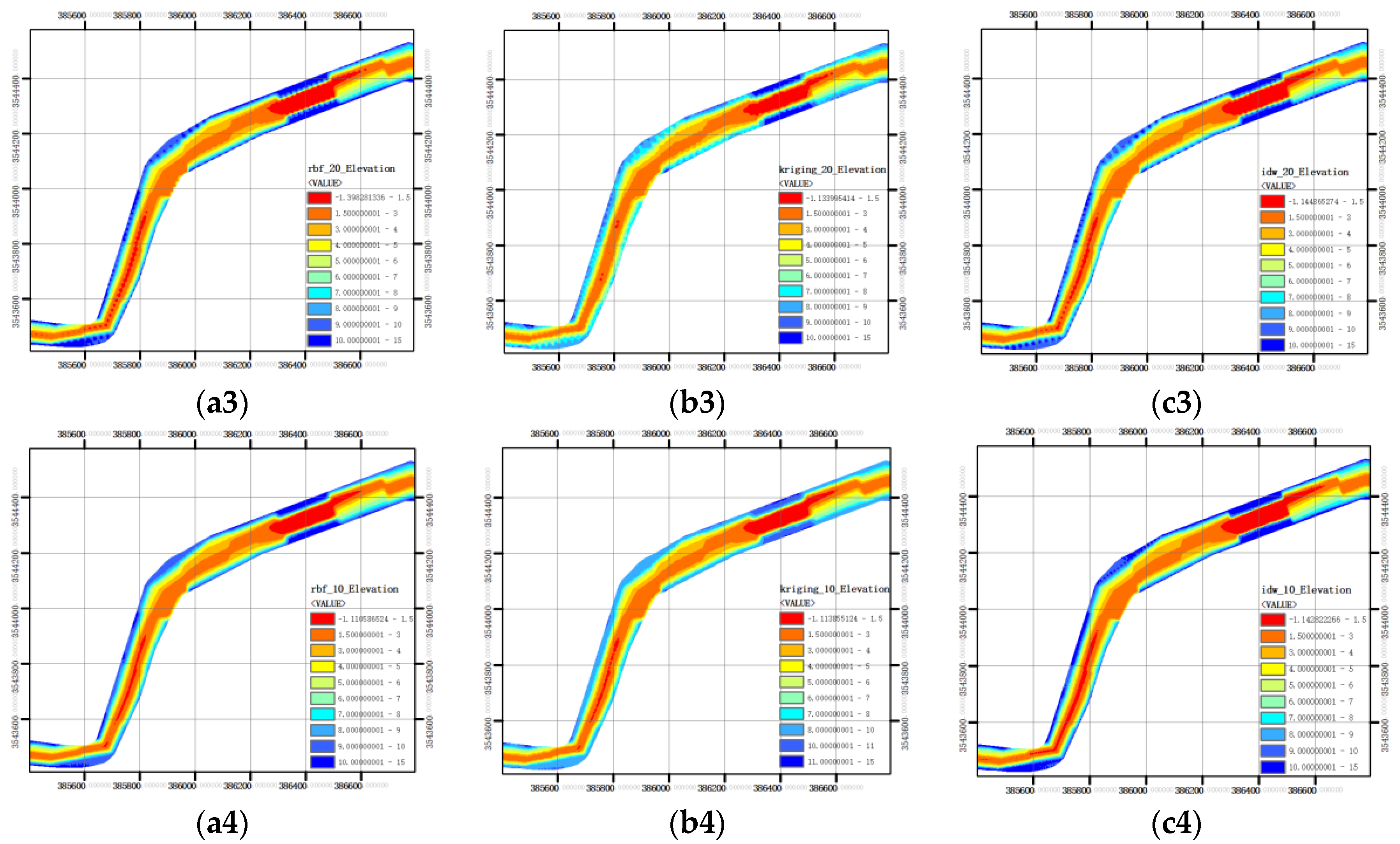
Figure 10.
Two-step interpolation results after preliminary encryption at different transverse spacing and further interpolation with RBF, Kriging, and IDW under CGCS2000 coordinate system. (a1,b1,c1) Transverse spacing of 80 m; (a2,b2,c2): 40 m as transverse spacing; (a3,b3,c3) 20 m as transverse spacing; (a4,b4,c4) transverse spacing of 10 m; (a1–a4) RBF as a further interpolation method; (b1–b4): Kriging as a further interpolation method; (c1–c4): IDW as a further interpolation method.


Figure 11.
Comparison of interpolation results using the same method with different intervals: (a) RBF; (b) Kriging; (c) IDW.
Figure 11.
Comparison of interpolation results using the same method with different intervals: (a) RBF; (b) Kriging; (c) IDW.


Figure 12.
Comparison of interpolation results of different sections with the same interval spacing (10 m): (a) Section 1; (b) Section 2; (c) Section 3; (d) Section 4.


Table 1.
The impact of section spacing on the spatial modeling results of underwater terrain.
| Spatial Interpolation Method | 200 m | 80 m | 40 m | 20 m | 10 m | |||||
|---|---|---|---|---|---|---|---|---|---|---|
| MAE (m) | RMSE (m) | MAE (m) | RMSE (m) | MAE (m) | RMSE (m) | MAE (m) | RMSE (m) | MAE (m) | RMSE (m) | |
| IDW | 2.46 | 2.87 | 0.77 | 1.01 | 0.62 | 0.80 | 0.91 | 1.05 | 0.21 | 0.30 |
| RBF | 3.00 | 3.70 | 0.82 | 1.03 | 0.86 | 1.12 | 0.90 | 1.12 | 0.50 | 0.38 |
| Kriging | 2.60 | 2.97 | 1.67 | 2.24 | 1.05 | 1.28 | 0.94 | 1.06 | 0.53 | 0.63 |
Publisher’s Note: MDPI stays neutral with regard to jurisdictional claims in published maps and institutional affiliations. |
© 2022 by the authors. Licensee MDPI, Basel, Switzerland. This article is an open access article distributed under the terms and conditions of the Creative Commons Attribution (CC BY) license (https://creativecommons.org/licenses/by/4.0/).
Share and Cite
MDPI and ACS Style
Liang, Y.; Wang, B.; Sheng, Y.; Liu, C. Two-Step Simulation of Underwater Terrain in River Channel. Water 2022, 14, 3041. https://doi.org/10.3390/w14193041
AMA Style
Liang Y, Wang B, Sheng Y, Liu C. Two-Step Simulation of Underwater Terrain in River Channel. Water. 2022; 14(19):3041. https://doi.org/10.3390/w14193041
Chicago/Turabian StyleLiang, Yan, Bo Wang, Yehua Sheng, and Changqing Liu. 2022. "Two-Step Simulation of Underwater Terrain in River Channel" Water 14, no. 19: 3041. https://doi.org/10.3390/w14193041
Note that from the first issue of 2016, this journal uses article numbers instead of page numbers. See further details here.