How Complex Groundwater Flow Systems Respond to Climate Change Induced Recharge Reduction?

Abstract

Our recent knowledge about the role of different fluid driving forces in the response of groundwater flow systems to climate change is still limited. This current study aimed to evaluate possible spatial and temporal changes in complex, gravity- and overpressure-driven groundwater flow systems induced by climate change and look for general trends and characteristics of the flow field using 2D transient groundwater flow simulations. Results showed significant large-scale changes in the transient subsurface flow field and flow dynamics due to recharge reduction. Local gravity-driven flow systems are the most vulnerable to atmospheric processes, while overpressured regimes are expected to be independent of direct climatic variability. By the involvement of different degrees of overpressure, it was revealed that, as the degree of overpressure increases, the penetration depth of the topography-driven local flow systems decreases. The higher the overpressure, the lower the climate change-induced groundwater level decrease over time, suggesting the buffering effect of overpressure as a fluid driving force in the flow systems’ response to the changes in hydrologic parameters. The main novelty of the study is the involvement of different fluid driving forces in the evaluation with the combination of a regional scale investigation, which is unique in the context of climate change effects on groundwater systems.

1. Introduction and Objectives

Groundwater reserves, being a crucial water resource, have great importance in sustainable water management, which requires an effective prediction of future availability. Simultaneous changes in key hydrologic parameters, predicted by the reports of the Intergovernmental Panel on Climate Change (IPCC), can significantly modify groundwater replenishment [1,2]. Moreover, the relation between climate parameters and groundwater is considered more complicated than with surface water [3], partly because of the residence time of groundwater, which varies on a wide scale and is likely to delay, attenuate and disperse the effects of climate change [4,5,6,7].

Climate variability will likely have diverse effects on subsurface recharge rates and mechanisms [2,6,8,9,10], as recharge is a sensitive function of the hydrological factors, local geological conditions, topography and land use. While many studies have predicted reduced subsurface replenishment [11,12], the effects of climate change on recharge may not necessarily be negative in all aquifers [13,14,15].

As scientific interest regarding the influences of climate change on groundwater systems has significantly increased over the last decade, it has been confirmed that both changes (i.e., decrease and increase in recharge) can have widespread consequences on subsurface conditions and groundwater systems. Several investigations have been completed to clarify possible future groundwater level changes [16,17], modification of groundwater recharge and storage [18,19], groundwater quality changes [20], alteration in subsurface temperature conditions [21], and in surface water–groundwater interaction [22,23]. However, the majority of the prior studies focus mainly on the hydrological aspects of climate change and the groundwater systems, while studies which deal with possible spatial and temporal changes in groundwater flow pattern and flow dynamics, i.e., in the fragmentation and hierarchy of nested flow systems, are still under-represented. Additionally, our recent knowledge about the role of the different fluid driving forces in the response of groundwater flow systems to climate change is still limited. A particularly interesting situation occurs when the groundwater flow pattern of a given area is determined by various fluid driving forces, because their exposure to changes in hydrologic parameters may be quite different. Gravity-driven flow is induced by elevation differences in the water table [24], owing to the most conspicuous consequences of alteration in atmospheric processes, as it is recharged directly by the infiltrating precipitation. Beyond topography, water movement in the subsurface can also be driven by stress-related mechanisms (such as sedimentary loading, tectonic loading and stresses, erosional unloading) and buoyancy (arising from density gradients due to changes in salinity and temperature) [25,26], which usually have weak and highly delayed, or do not have a direct connection with the surficial hydrologic processes.

This study aimed to contribute to the understanding of the large-scale behaviour of such complex subsurface processes in response to climate change-induced recharge reductions by looking for general trends and characteristics of the flow field using 2D transient groundwater flow simulations.

The Duna–Tisza Interfluve in Hungary was assigned as a sample area, where two separated flow domains were identified and deeply studied [27]. The upper gravity-driven flow regime is recharged directly from the infiltrating precipitation, while the underlying overpressured domain is maintained by pore volume reduction due to compaction and tectonic compression of the basement [28,29]. Such flow regimes do not have meteoric water recharge, as the super-hydrostatic vertical pressure component prevents vertical leakage from above [30].

In the study, special emphasis was put on (i) how the relative role of the two fluid flow systems (i.e., gravity-driven and overpressured domain) may change, (ii) how the hierarchy and fragmentation of the ground flow field may alter by time, (iii) how the penetration depth of the upper, gravity-driven flow field may adjust to these changes and (iv) how groundwater-related shallow surface water bodies will be affected by these changes.

The novelty of the study is the regional scale of the investigation, which is subordinate in the literature compared to the lower scale, site-specific predictions. It requires a different approach, and in parallel, combined with a relatively long-term investigation (several decades), it could provide more extensive spatial and temporal information on the effects of climate change on groundwater flow patterns and dynamics, which is still underrepresented in the previous studies. Additionally, the involvement of different fluid driving forces in the evaluation is unique in the context of climate change effects on groundwater flow systems.

2. Sample Area

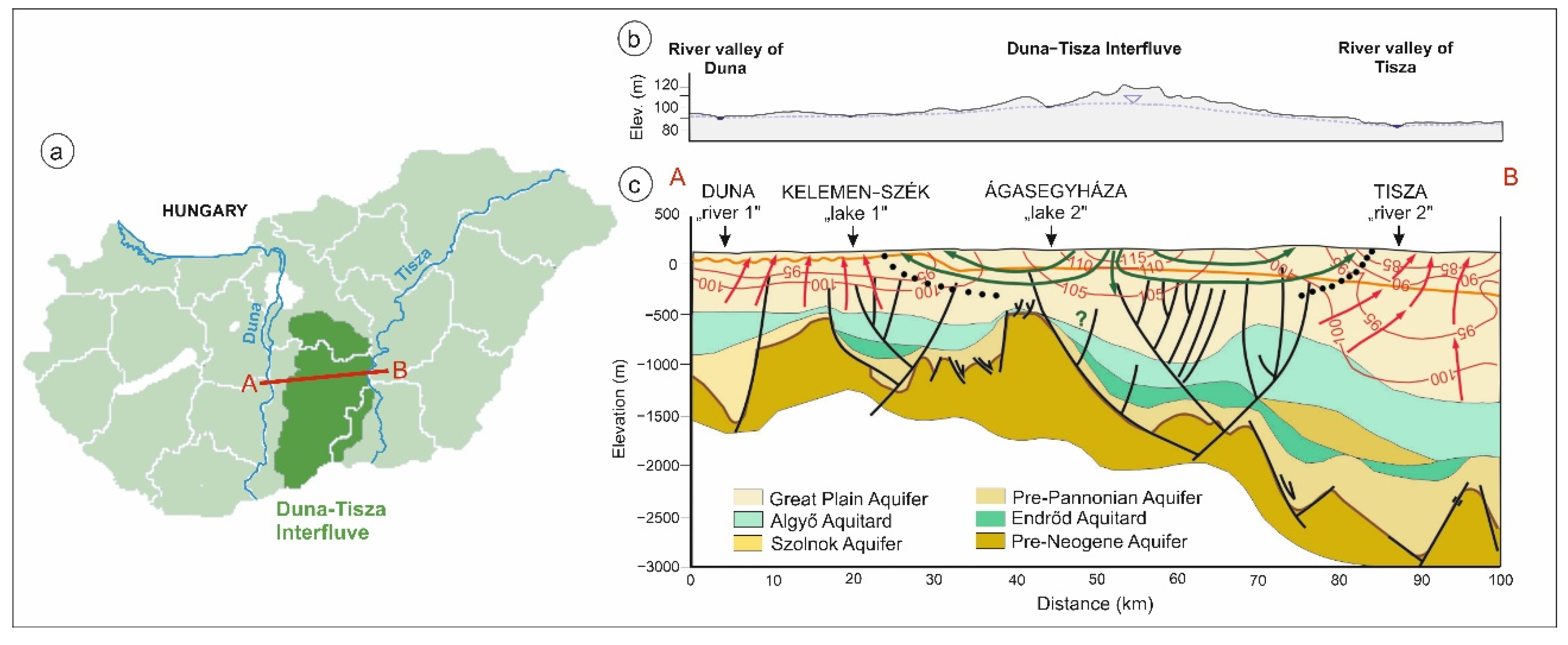
The Duna-Tisza Interfluve, located in Hungary, is characterized by flat-bottomed valleys at the River Duna and Tisza (80–95 m asl), and by a N-S orientated central ridge (100–130 m asl) along the divide (Figure 1).

The eastward-dipping basement of the broader area is tectonically strongly disturbed and characterised by horst and graben topography. It is covered by Neogene semi- to unconsolidated marine, deltaic, lacustrine, fluviatile and eolian clastic sediments with a thickness from 600 m at the Duna River to over 4000 m at the Tisza River [31]. Their hydraulic properties were determined by qualitative estimation derived from lithological and facies conditions [27,29].

Hydrostratigraphically, the rock framework is divided into an upper and a lower sequence by an extensive aquitard (Algyő Aquitard) of an average hydraulic conductivity of K = 10⁻⁸ ms⁻¹. The aquitard is overlain by a highly permeable aquifer (Great-Plain Aquifer) including two geological sequences, which can be characterised together by an average hydraulic conductivity of K = 10⁻⁵ ms⁻¹ [27]. It mainly consists of fluvial, eolian and lacustrian formations interrupted by local low-permeable eolian and lacustrine ones. The lower series of units consist of Neogene siltstones, sandstones and clays (Szolnok Aquifer and Endrőd Aquitard with hydraulic conductivities varying between 10⁻⁹ and 10⁻⁶ ms⁻¹) underlain by the Pre-Pannonian Aquifer (with an estimated hydraulic conductivity of 10⁻⁶ ms⁻¹), and Pre-Neogene formations consist of carbonates, metamorphic formations and flysch with unknown hydraulic properties [32] (Figure 1).

Based on detailed hydraulic studies by previous authors, the principal features of subsurface flow conditions of the Duna-Tisza Interfluve are relatively well-known. Two different but hydraulically connected, superimposed groundwater flow domains are acting: an upper gravity-driven meteoric fresh water, which can be characterised by near-hydrostatic pressure conditions and an underlying overpressured domain of water with high total dissolved solid (TDS) content [27,29,33].

The groundwater flow in the upper aquifer is controlled by the topography, causing a downward flow beneath the highlands and an upward flow beneath the valleys. The underlying overpressured system is characterized by an upward vertical flow component, which is maintained by pore volume reduction due to compaction and tectonic compression of the basement [27,28,29,34,35]. The upward overpressured flow is forced and deflected by descending fresh meteoric waters of the central regions toward the river valleys, where they are discharging. The distribution patterns of freshwater and saline vegetation and the location of salt-affected soils, as well as the hydrochemical differences of fresh and saltwater lakes at relatively short distances from each other, reflect the different properties of the vertically superimposed gravity-driven and overpressured flow systems [27,36,37]. Lakes of the Interfluve are situated in really extensive shallow (<1 m deep) depressions and are not affected by recharging or discharging stream water.

Hydraulic communication between the upper gravity-driven and underlying overpressured systems occurs by diffusion and seepage across the aquitard through permeable, discrete structural and sedimentological discontinuities [27,29,36,38].

As the upper, gravity-driven groundwater flow system is recharged directly from the infiltrating precipitation, this flow regime is regionally renewable on a human and on a geological timescale as well [27,29]. In contrast, the deep flow regime, being a hydraulically closed system, is not replenished by precipitation, because vertical leakage from above is restricted by the excess (above hydrostatic) vertical pressure [29,30]. Consequently, this pressure regime is characterized by fluids which are not renewable [30]; the amount of water which can be released depends on the elastic properties of water and rock matrix, i.e., the regional storage capacity of the system [39,40].

Predicted Climate Change and Consequences on Groundwater Recharge

The Duna-Tisza Interfluve is characterised by a moderately continental climate with approx. 600 mm annual precipitation and a 10 °C average annual temperature. Based on regional climate predictions for Hungary, the annual precipitation is likely to decrease by about 20% by the end of the century [41], while the annual temperature is likely to increase by 4–5.4 °C [42] compared to the reference period of 1961–1990.

Focusing on the large-scale alterations of groundwater flow pattern and dynamics rather than site-specific absolute predictions of future groundwater levels, the most deterministic hydrologic parameters, i.e., precipitation and evapotranspiration (described by dynamic factor analysis of Király [43] were taken into account during the evaluation of groundwater recharge. Overland flow and through-flow were neglected, considering that rainfall rate rarely exceeds infiltration capacity under recent climatic conditions of the area; moreover, the runoff would also decrease in time due to decreasing precipitation.

In the case of the Interfluve, the Duna and Tisza rivers represent a regional hydraulic potential minimum of the area. Due to the groundwater flow characteristics of the sample area, the effects of the rivers on groundwater level can be detected mainly in their vicinity [27], and therefore, surface runoff was not taken into consideration during recharge calculation.

It is assumed that uncertainties generated by this site-specific simplification are not significant compared to the uncertainties inherent in the climate change predictions and the numerical investigation can, nevertheless, help to gain insight into the large-scale response of the different groundwater flow systems to the predicted climate change.

Evapotranspiration was calculated based on the simplified Turc formula [44], which requires only limited data and is simple to implement, and given as:

$$E=\frac{P}{\sqrt{0.9+\frac{P^2}{K^2}}}$$

(1)

where E is evapotranspiration (mm yr⁻¹), P is annual precipitation (mm yr⁻¹), K = 300 + 25T + 0.05T³ and T is the mean annual air temperature (°C).

Assuming P = 600 mm yr⁻¹ and T = 10 °C, which are characteristic of the area, the current evapotranspiration (E) is 435 mm yr⁻¹. Subtracting E from precipitation (P), the current groundwater recharge is 165 mm yr⁻¹. Therefore, under current conditions, only approx. 27% of precipitation can reach the saturated zone and recharge the groundwater system.

In order to easily follow the recharge reduction-induced changes in the subsurface flow processes, a pessimistic scenario was taken into account with a 20% decrease in annual precipitation and a 4 °C increase in mean annual temperature, which can lead to a significant, >60% decrease in recharge by the end of the century (2100) in the case of the sample area.

3. Numerical Simulation Method

In the current study, future modifications of groundwater flow system characteristics due to climate change were simulated using the transient numerical flow module within the Heatflow-Smoker code [45] along a 2D vertical plane. Heatflow-Smoker is a finite element code, which couples density-dependent groundwater flow and heat transport.

The model solves the continuity equation for flow [46] which can be expressed as:

$$\frac{\partial }{\partial x_i}\left[K_{i,j}\left(T\right)\left(\frac{\partial \Psi }{\partial x_j}+{\rho }_r\left(T\right)\times \overline{n_j}\right)\right]=S_s\frac{\partial \Psi }{\partial t}$$

(2)

where x_ij are the 3D spatial coordinates (m), K_ij(T) is the temperature-dependent hydraulic conductivity tensor (m s⁻¹), ψ is the equivalent freshwater head (m), ρ_r(T) is the temperature-dependent relative density of water (-), S_s is the specific storage (m⁻¹) and t is time (s).

Changes in flow patterns were followed along a heterogeneous, anisotropic, two-dimensional vertical section across the Interfluve (Figure 1 and Figure 2). The 100 km long and 1500 m deep model domain was subdivided into a regular network of 1000 × 15 elements in the x and z directions, with each rectangular prism element measuring 100 m × 100 m, respectively (with 1 element in the transverse dimension).

As a first step, a steady-state simulation was run based on site-specific hydraulic and hydrostratigraphic data, representing the current groundwater flow system. The full transient simulation was run over a period of 80 years, with a time step of 1 yr. Changes to the hydrologic parameters were based on referenced climate change predictions.

Since our interest was to highlight the possible influence of climate change on complex groundwater flow systems—driven by gravity and overpressure—and look for general characteristics of the transient flow field, some simplifications were included in the simulation approach, which was not expected to be significant in terms of the objectives of the study.

3.1. Model Dimensionality

It is obvious that representing a 3D real system as a two-dimensional cross-section overlooks some system dynamics. However, depending on the system characteristics, the scale of the investigation and the questions to be answered, in some cases a two-dimensional approach could be a suitable choice. For low-relief settings (i.e., with a flank slope < 10°), where the ratio of recharge (R) to hydraulic conductivity (K) of the uppermost subsurface layer is <0.15, 2D cross-sectional models may be justifiable since transverse flow (i.e., perpendicular to the primary regional topographic gradient) would be generally less than 10% of the total flow [47]. As in the case of the sample site, the R/K ratio is below the critical value; furthermore, the general characteristics of the dynamically changing flow regimes are the focus of the investigation, and a 2D model is considered a reasonable approach for providing the needed insight into the response of the system to the predicted changes of the key hydrologic parameters.

3.2. Driving Forces on Groundwater Flow

The current numerical investigation focuses on the influences and temporal changes of the water table gradient (i.e., gravity) and sediment compaction-induced overpressure was the focus of the investigation. In the case of the Duna-Tisza Interfluve sample area, possible effects of density-driven flow due to high total dissolved solids (TDS) concentrations and temperatures on the flow field were analysed by previous authors. It was revealed, that (i) due to the 45–50 °C km⁻¹ geothermal gradient of the area, heat can be taken into account as a driving force, but it has only a small modifying effect on the regional groundwater flow pattern of the area [48]; (ii) TDS of groundwater remains below 40 g L⁻¹ in the case of the Interfluve [27,38]; and (iii) the effects of a high geothermal gradient and a relatively low-dissolved solid content of the water can equalize each other [49]. Therefore, the influence of a buoyancy-driven force was not considered during the current study and an isothermal groundwater flow was simulated, assuming a uniform temperature of 10 °C and water density of 1000 kg m⁻³.

3.3. Representation of Overpressure

In the case of gravity-driven flow systems, subsurface hydraulic potential distribution is clearly determined by the groundwater table and flow is generated by its gradients [24]. Therefore, hydraulic head (h) values in a given basin are limited by the range of the groundwater table elevation (z_wt,min and z_wt,max, by noting that in the case of groundwater table, its elevation and hydraulic head is equal, z_wt = h_wt) and spatial distribution pattern of fluid-dynamic parameters representing normal, i.e., near-hydrostatic pressure conditions. Any alteration in subsurface pressure conditions is due to the gravitational flow of groundwater [39], i.e., pore pressures are adjusted to their hydrogeologic environment (equilibrium-type overpressure, [50]).

In general, abnormal fluid pressure is generated by transient processes, such as stress changes caused by tectonic compression and/or disequilibrium compaction; changes in fluid volume due to thermal expansion, diagenetic and metamorphic processes as well as hydrocarbon generation; or fluid movement due to density differences caused by buoyancy forces and osmosis [50,51,52,53,54,55]. In many sedimentary basins, stress-related mechanisms are the most likely causes of overpressure (OP), which is abnormally high pressure in the subsurface that exceeds the hydrostatic pressure at a certain depth.

Overpressures are created whenever the rate of pressure generation exceeds the rate of pressure dissipation. The rate of fluid-pressure dissipation across a porous medium is inversely proportional to the hydraulic conductivity of that medium. Therefore, low-conductivity regions are essential for the generation and maintenance of overpressures [50], as they could function effectively in units where sufficiently low-permeability formations are present, which inhibits the complete dewatering of the underlying formation and contributes to the excess pressure of the pore fluid [52].

According to the definition by Mádl-Szőnyi [56], overpressure conditions prevail if the deviation of the measured dynamic pore pressure (p_dyn) from the static pore pressure (p_st), characteristics for the given elevation, exceeds the limit of near-hydrostatic pressure conditions (∆p_hydrostatic). It can be given as:

$$p_{dyn}>p_{st}\pm \Delta p_{hydrostatic}=p_{st}\pm \left(\rho g\frac{z_{wt,max}-z_{wt,min}}{2}\right)\times {10}^{-6}$$

(3)

where ρ is the density of water (1000 kg m⁻³), g is the acceleration due to gravity (9.81 ms⁻²) and z_wt,max and z_wt,min are the maximum and minimum elevations of the groundwater table [m].

Based on Equation (3), abnormal pressure can be determined simply by the hydraulic head interval of groundwater level of the given basin, as h > h_wt,max represents overpressure, while h < h_wt,min is the characteristic for underpressure conditions.

In a recent study, an overpressured system is characterized by an upward vertical flow, which is maintained by pore volume reduction due to compaction and tectonic compression of the basement of the sample site [29]. Therefore, overpressure is represented by an increased hydraulic head along the bottom of the system, induced by groundwater inflow across the bottom of the studied Section 3.4. Input parameters, initial and boundary conditions of the model.

Considering the main aims of the study, i.e., the evaluation of the large-scale alterations of groundwater flow pattern and dynamics rather than a site-specific absolute prediction of future groundwater levels, a simplified hydrostratigraphic configuration was applied, focusing on the key elements of site-specific hydrogeological characteristics of the sample site. Therefore, a non-uniform thick aquitard and an overlying aquifer were tested. In order to provide a better resolution within the uppermost subsurface zone, where main changes are expected due to the recharge reduction-induced modification in the groundwater table; the aquifer was differentiated into three distinct sub-units (aquifer 1, 2 and 3, Figure 2b) in accordance with the hydrostratigraphic settings of the sample area. However, in the following interpretation, it is referred to uniformly as “aquifer”. Hydraulic parameters of the formations were defined based on the previous detailed hydrogeological evaluation of the Duna-Tisza Interfluve [27,29,36] (Figure 2b).

The numerical simulation was performed within the saturated zone, for which the groundwater table forms the upper surface, represented by the recent water table configuration of the sample site (Figure 2a). Across the upper flow boundary, outside of the river valleys and local lake areas with constant head, a specific recharge was defined, based on the recent hydrologic parameters for the steady-state simulation, as well as calculated by the model taking into consideration a linear decrease in recharge in the case of the transient model. Water inflow across the lateral boundaries represents groundwater movement toward the regional hydraulic potential minimum of the river valleys within the upper aquifer.

Upward overpressured flow from the underlying formations was represented by groundwater inflow across the lower flow boundary of a studied cross-section with different Darcy flux values in the case of the different simulated cases with a different degree of consequent hydraulic head increase. In the case of comparative simulations neglecting the effect of overpressure, the lower flow boundary was handled as no-flow, i.e., Darcy flux of q = 0 ms⁻¹ was applied (Figure 2b).

In the case of the transient simulation, the water table configuration obtained from the steady-state simulation was used as the initial condition for the transient flow model. Fixed heads assigned to represent the steady-state lake levels were eliminated; thus, the water table elevation change below the lakes was calculated by the model based on the predicted decrease in recharge across the top boundary over each time step. Comparisons of the simulated transient groundwater levels with local lakebed bottom elevations were used to follow the possible changes in surface water levels.

Rivers along the studied section represent the regional hydraulic potential minimum. As the Danube represents the second largest river in Europe, while the Tisza is its largest sub-catchment, their response to predicted climate change is difficult to predict and beyond the scope of this study. Effects of the rivers on groundwater levels in the case of the sample area can be detected mainly in their vicinity [27]. Moreover, in the case of the studied system with an elevated area between the main rivers, the relative hydraulic position of the rivers (i.e., minimum hydraulic potential) would remain in spite of any changes in river water level. Therefore, changes in rivers’ water level and streamflow under climate change were not considered. A sensitivity analysis of the effects of river water level reductions on the flow field showed no significant effects on the general conclusions of the study.

During the transient simulation, uniform specific storage of S_s = 0.001 m⁻¹ was applied, which represents a combination of relatively high storativity in shallow unconfined sediments (governed by porosity) and relatively low storativity in the deeper rock framework.

3.4. Simulated Cases

As an initial case, only gravity as a driving force was taken into account during the simulation, neglecting the effects of overpressured flow. With the help of these models, the effects of climate change-induced recharge reduction on a purely gravity-driven flow system can be analysed, and then its flow pattern and dynamic characteristics are easily comparable with the ones created by complex, gravity and overpressure-driven flow systems.

Different degrees of overpressure were also taken into account, in order to evaluate its relative role compared to gravity in canalising groundwater and also, its behaviour under the changing hydrological characteristics of the system. Considering the recent water level configuration of the sample area with h_wt,min = 83 m and h_wt,max = 110.4 m, abnormal pressure can be evaluated based on Equation 3, which denotes overpressure conditions at the bottom of the system (at 1500 m depth) with p_dyn > 15.6 MPa. Beyond a medium overpressure of 25 MPa at the bottom, characteristics for the sample area, effects of a lower (20 MPa) and a synthetic case with extreme high (65 MPa) overpressure were tested for comparison by applying a corresponding groundwater inflow across the bottom of q_in(bottom) = 5 × 10⁻¹¹ ms⁻¹ (lower OP), 10⁻¹⁰ ms⁻¹ (medium OP) and 5 × 10⁻¹⁰ ms⁻¹ (higher OP).

The numerical investigation aimed to look for general trends and characteristics of the transient flow field and focused on (i) how the relative role of the two fluid flow systems may change due to climate change-induced recharge reduction, (ii) how the hierarchy and fragmentation of the flow field may alter and (iii) how the penetration depth of upper, gravity-driven flow field may adjust to these changes. Due to the scale of the investigation, local predictions of absolute surface water level changes are beyond the scope of the study. However, as surface waters are an integral part of the groundwater flow systems, comparisons of the simulated transient groundwater levels with shallow (<1 m deep) local lakebed elevations can be used to follow the possible changes in lake water levels during the transient simulations and predict their future state: (i) will they likely be maintained or will they eventually be drying, and (ii) will they be affected by the possible changes of their interconnected groundwater systems?

4. Results

4.1. Pure Gravity-Driven Groundwater Flow Systems in a Changing Climate

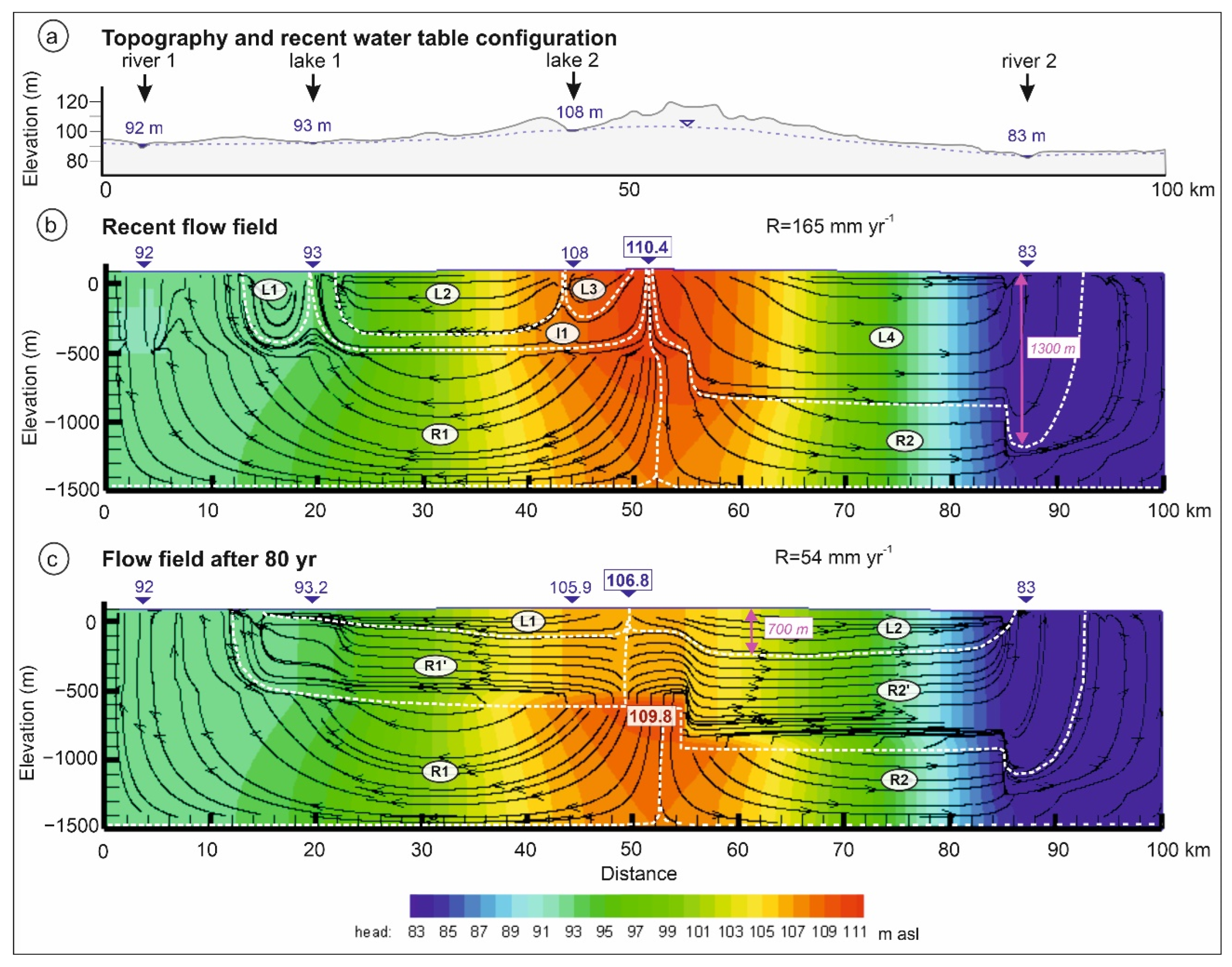
Considering only the effect of gravity as the driving force, groundwater flows from the elevated ridge to the river valleys in accordance with the hydraulic head differences and hydraulic conductivities. The flow field is characterised by hierarchically nested flow with local (L1, L2, L3, L4), intermediate (I1) and regional (R1, R2) flow systems, determined by the water table (Figure 3). Groundwater recharge takes place along the elevated ridge by the infiltrating precipitation, while discharge occurs dominantly along the river valleys within relatively broad zones. The developed flow field is hydraulically separated by a subsurface water divide below the main recharge area of the ridge (at approx. 51 km distance, Figure 3b). Gravity-driven flow is settled into a more dynamic upper flow field in the aquifer with a maximum flow velocity of 2 × 10⁻⁶ ms⁻¹, and a much slower system in the aquitard with a maximum Darcy flux of 10⁻¹⁰ ms⁻¹. It is a major part of the infiltrating water moving in the upper aquifer arranged into local or intermediate systems (L1, L2, L3, L4, I1, Figure 3b), reaching a maximum penetration depth of 1300 m.

As results of the transient simulation showed, recharge reduction (from 165 mm yr⁻¹ to 54 mm yr⁻¹, calculated based on the predicted climate change) led to large-scale changes in the gravity-driven flow field. Water level change was the highest at the watershed below the recharge area, where it decreased by at most 3.6 m after 80 yr, leading to the extent of the hydraulic potential drop within the aquifer. However, due to the significantly lower diffusivity of the aquitard unit (D, ratio of hydraulic conductivity K to specific storage S_s), its hydraulic head distribution was not affected by the recharge reduction. Consequently, a hydraulic potential maximum (h_max = 109.8 m) developed within the aquitard below the subsurface water divide of the system (at approx. 51 km distance and 700 m depth), which is 3 m higher compared to the maximum hydraulic head of 106.8 m along the water table, i.e., transient processes induced by recharge reduction led to the development of a slight overpressure within a gravity-driven flow system.

This situation created an upward flow domain within the lower part of the aquifer in accordance with the hydraulic head distribution. With these changes, direct surface replenishment of the regional flow systems (R1, R1′, R2 and R2′, Figure 3c) from infiltrating precipitation ceased. In parallel, flattening of the water table led to a decreased fragmentation in the uppermost flow domain (from L1, L2, L3, L4 local and I1 intermediate flow systems to L1 and L2 local ones), and to a significant decrease in the penetration depth of the infiltrating water from 1300 m (characteristic for the initial flow field, Figure 3b) to 700 m (Figure 3c).

Simulated groundwater level changes suggest that the water level of lake 1, which takes place at the lower flank of the ridge, will not be significantly affected by the recharge reduction after 80 yr in the case of a pure gravity-driven system. However, its feeding flow system would be changed over time from a deeper, intermediate system (I1 with a penetration depth of 600 m, Figure 3b) to a shallower, local one (L1 with a penetration depth of 300 m, Figure 3c). Another clear result of the transient simulation was the continuous decrease in groundwater level below lake 2, which dropped 2.1 m after 80 yr, i.e., its lakebed was dried.

4.2. Effect of Decreasing Recharge on a Combined Flow System with Gravity-Driven and Overpressured Flow Domains

After the evaluation of the effects of recharge reduction on a pure gravity-driven flow system, the effect of an underlying overpressured flow regime was involved in the investigation, and the response of the different flow systems to climate change was analysed and compared to each other.

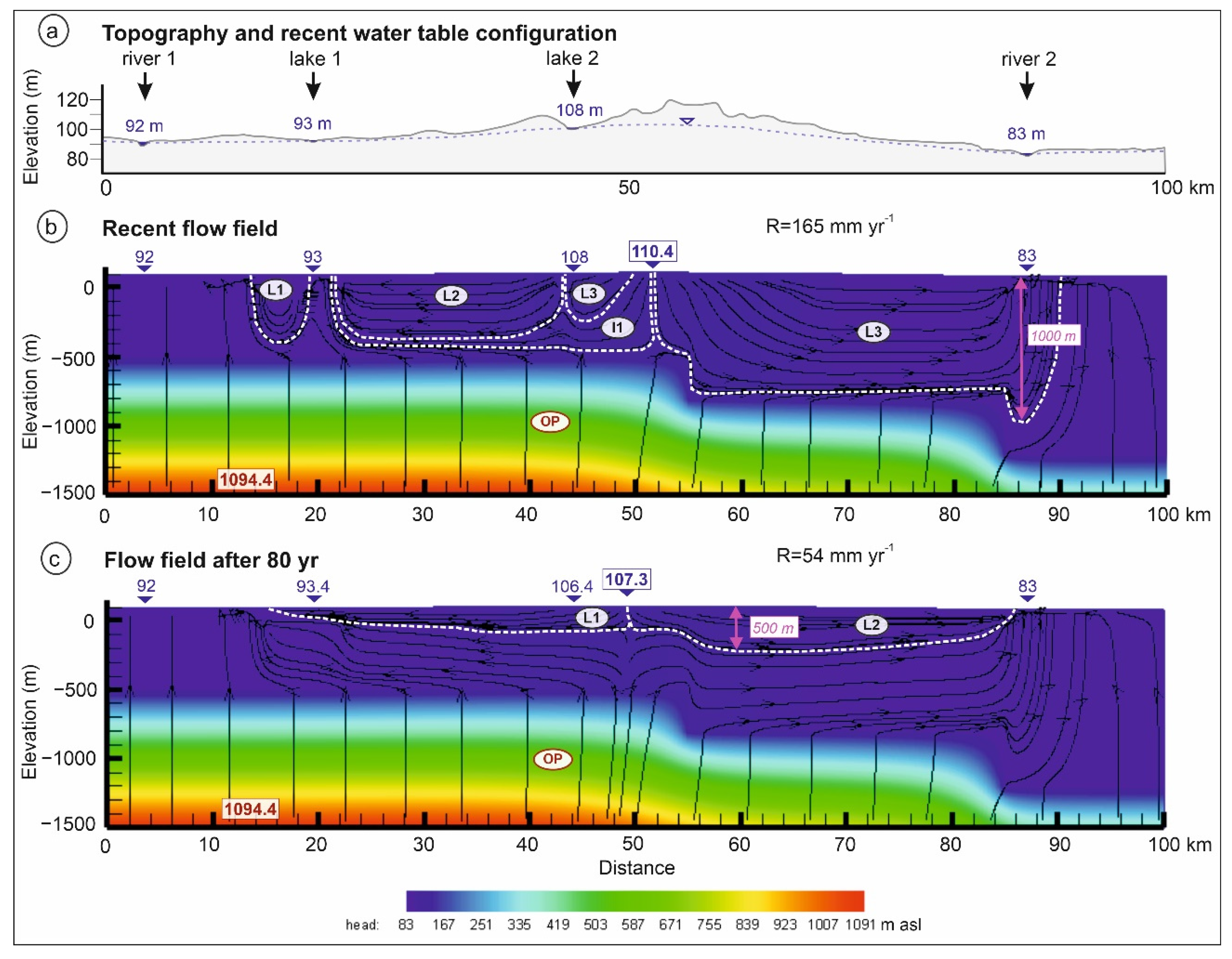
The flow field of the combined flow system consists of an upper, hierarchically nested gravity-driven flow with local and intermediate flow systems (L1, L2, L3, I1, Figure 4a) reaching a maximum penetration depth of 1000 m (L3), which is vertically superimposed with a domain of an upward overpressured flow. Latter is developed by a uniform groundwater inflow of 10⁻¹⁰ ms⁻¹ across the bottom of the system, leading to a significant hydraulic head increment with h_max = 1094.4 m (corresponding to p_dyn of 25 MPa). Consequently, flow pattern and dynamics significantly changed in the aquitard compared to the pure gravity-driven case; the flow direction reversed and in parallel, the maximum Darcy flux increased by two orders of magnitude (from 10⁻¹⁰ ms⁻¹ to 1.1 × 10⁻⁸ ms⁻¹). However, since groundwater table elevation, representing recent conditions, is the same as it was in the case of the pure gravity-driven flow system analysis, the main characteristics of the current steady-state flow models, including neglecting and considering the effect of the underlying overpressured flow, are very similar within the aquifer. Its flow field is hydraulically separated by the subsurface water divided below the recharge area (at approx. 51 km, Figure 4b). Groundwater in the aquifer flows toward the potential minimums represented by the river valleys with a maximum fluid flux of 2.1 × 10⁻⁶ ms⁻¹, owing to similar recharge and discharge characteristics compared to the pure gravity-driven case. One remarkable difference appears below lake 1, which is fed by the overpressured upward flow in this case (Figure 4b); on the contrary, it is recharged directly by the infiltrating precipitation, transported by an intermediate flow system in the pure gravity-driven case (Figure 3b).

As a result of the recharge reduction, the groundwater table dropped by 3.1 m after 80 yr, which is 0.5 m lower compared to the water level decrease in the pure gravity-driven case. In parallel, fragmentation of the upper gravity-driven flow system decreased to single local cells with a maximum penetration depth of 500 m (L1, L2, Figure 4c). Flow direction and dynamics within the aquitard were not affected by these changes. However, the boundary between the overpressured and the superimposed gravity-driven flow domain was shifted from the strata boundary (recent case, Figure 4b) to a shallower depth after 80 yr (Figure 4c). The flow direction of overpressure-driven upward flow, thus, deviated within the aquifer in accordance with the higher hydraulic conductivity of this unit and the subsurface hydraulic gradient forced it toward the river valleys, and consequently, the proportion of horizontal flow increased.

Results of the transient simulation also highlighted major changes, which could affect the future state of the lakes. Discharge of overpressured flow into lake 1 will be eliminated due to recharge reduction within the next 80 yr. In the case of the Duna-Tisza Interfluve sample area, where overpressured upward flow contains a high amount of total dissolved solids, it could have significant effects on the quality of the surface waters, and also on the distribution of saline vegetation and soils. In parallel, the groundwater table changes suggest a slight increase (0.4 m, Figure 4c) in lake water level after 80 yr. In contrast, the groundwater level drop of 1.6 m below lake 2 (from 108 m to 106.4 m, Figure 4b,c) is predicted by the model, i.e., it will eventually be dry after 80 yr.

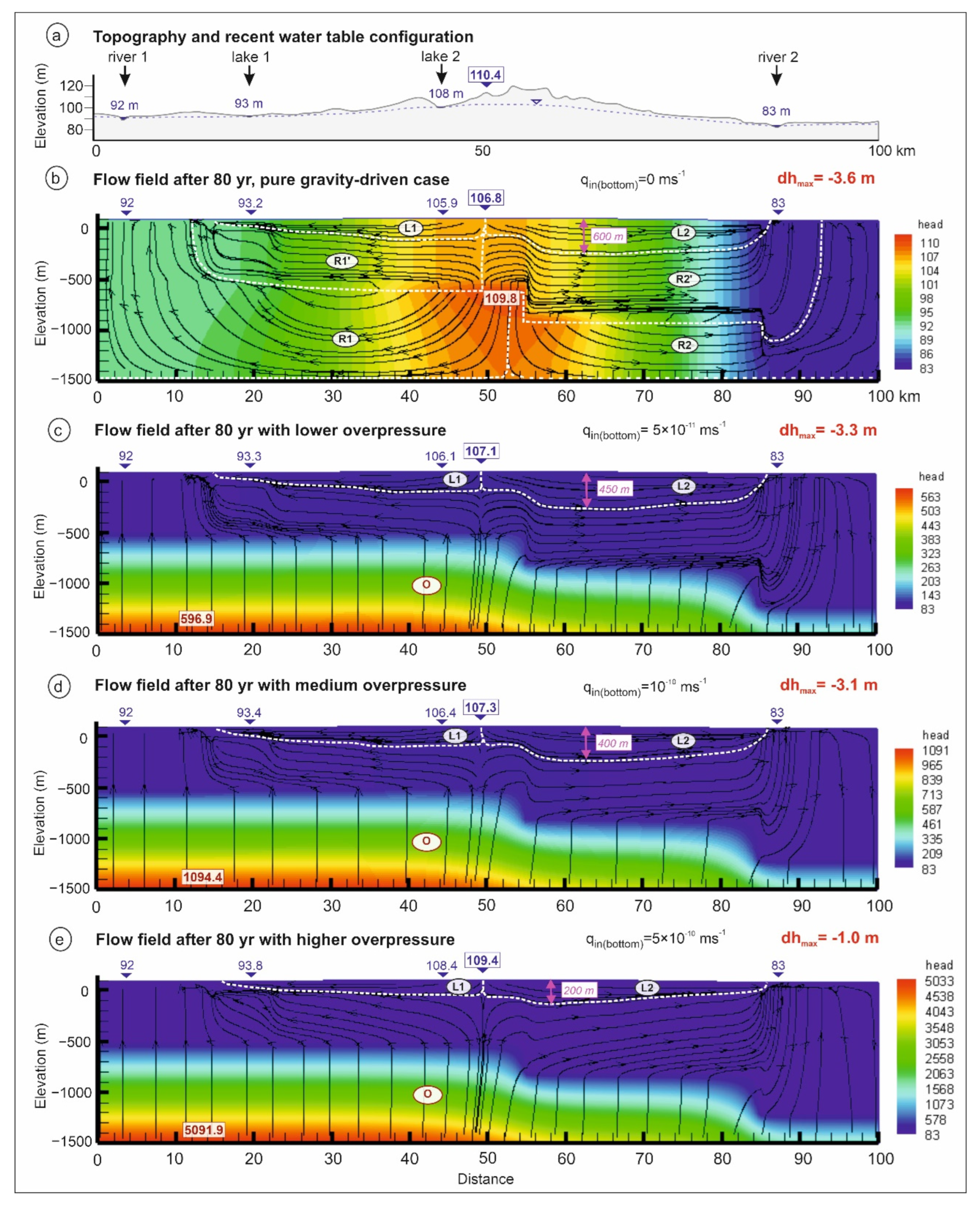
As a next step, different degrees of overpressure were involved in the numerical investigation, in order to evaluate the relation of gravity and overpressure as driving forces in canalizing groundwater and its effects on the transient flow field under changing climatic conditions. The simulated case with “medium” overpressure of 25 MPa at the bottom of the system (induced by groundwater inflow of q_in(bottom) = 10⁻¹⁰ ms⁻¹ Darcy flux across the lower boundary, Figure 4c and Figure 5d) represents the conditions that prevailed in the Duna-Tisza Interfluve sample area. As a comparison, the lower overpressure of 20 MPa (induced by q_in(bottom) = 5 × 10⁻¹¹ ms⁻¹ influx) and a synthetic case with extreme high overpressure of 64 MPa (induced by q_in(bottom) = 5 × 10⁻¹⁰ ms⁻¹ influx) was also tested.

As the results showed, the degree of overpressure at the bottom of the system clearly determines the penetration depth of the upper, topography-driven flow system, which represents, at the same time, the boundary between gravity- and overpressure-driven flow domains. As the degree of overpressure (and consequent hydraulic head increment at the bottom) increases, the penetration depth of the topography-driven local flow systems decreases (e.g., from 600 m without overpressure to 200 m with high overpressure in the case of the L2 system, Figure 5). In parallel, the drop of groundwater level was obviously affected by the magnitude of upward overpressured flow. Recharge reduction led to a 3.6 m decline in the pure gravity case, while to a 3.1 m water level drop involving medium overpressure (represents characteristics similar to the sample area), and even to a smaller, 1.0 m decrease in the case of the highest overpressure (Figure 5), showing that the higher the overpressure, the lower the groundwater level decrease over time. As a consequence, changes in surface water levels are also affected, as proven by the opposite change in the case of lake 2 with the highest overpressure case (0.4 m water level rise, Figure 5b) compared to the pure gravity simulation (2.1 m water level drop, Figure 5e).

By modifications in the groundwater table in the different tested cases, alterations in flow dynamics can also be followed. By increasing the degree of overpressure, the average Darcy fluxes gradually increased compared to the fluxes of the pure-gravity case. Major changes in flux can be observed in the vertical direction in both the aquifer (aquifer 1, 2 and 3, Figure 2b) and in the underlying aquitard. However, the magnitude of flux changes is different in the high hydraulic conductivity aquifer and in the aquitard characterized by low hydraulic conductivity (Figure 6).

5. Discussion

The 2D transient groundwater flow simulation study carried out focused on understanding the effects of decreasing recharge due to climate change. The most conspicuous changes highlighted by the transient simulation were groundwater level decrease and modification of the flow system hierarchy along the studied section in both tested cases, i.e., neglecting and considering the effect of overpressure as a driving force. Water level change was highest at the watershed below the ridge, decreasing toward the river valleys. It is consistent with the findings of Zhao et al. [57], who examined the transient behaviour of nested flow systems and found that water table fluctuations are greatest near the flow divides and are less variable in the main discharge areas. Peters et al. [58] also found that long periods of dry climate had a greater effect on suppressing the groundwater level near the groundwater divide (i.e., the recharge area).

The results showed that as the groundwater level decreases, the hierarchically nested flow field gradually degrades over time, which leads to a less fragmented system with single local cells (Figure 3c and Figure 4c). This is in agreement with the conclusions of Liang et al. [59], who showed that, as groundwater recharge gradually decreases, the flow pattern changes from (i) a fragmented flow field with separated local cells, to (ii) a less fragmented flow field with nested flow systems (including local, intermediate and regional cells) and to (iii) a single regional flow cell. These changes have clear effects on lake water levels and their replenishment by groundwater. Moreover, due to the alteration of subsurface potential distribution—induced by groundwater level changes—penetration depth of infiltrating meteoric water was decreased, and flow intensity and velocity was reduced. Zhou et al. [60] also concluded that the response of the groundwater level to linearly varying climate change shows spatial variability, which obviously affects groundwater flow velocity as well.

Beyond the large-scale changes in flow system dimensions and the relationship between local, intermediate and regional flow systems, the degree of consequential modifications on the flow field is quite different in the case of combined flow systems (i.e., with gravity-driven and overpressured flow domains) compared to pure gravity-driven flow systems, highlighting the modifying effects of overpressure.

Water level decrease was highest (d_hmax = −3.6 m, Figure 5) in the case of the pure gravity-driven simulation, which was moderated by the involving overpressured flow. As the results of the numerical investigation highlighted, the higher the degree of overpressure at the bottom of the system, the lower the decrease in groundwater level after 80 yr. In parallel, the magnitude of upward overpressured flow clearly determines the penetration depth of near-surface local flow systems, which is the deepest in the pure gravity-driven case and gradually decreases with the increase in overpressure (from 600 m to 200 m, Figure 5). It was also revealed that as the flow intensity of a shallow gravity-driven flow system decreased, the relative role of overpressure started to increase, and could buffer the effects of recharge reduction on groundwater levels depending on the degree of overpressure. These results are novel, as the involvement of different fluid driving forces in the analysis of climate change effects on groundwater flow systems is unique.

Another question addressed to the effects of modified flow patterns on groundwater-related shallow surface water bodies (Figure 1). Simulated groundwater level changes suggest differences between lake 1 and lake 2 in terms of their response to recharge reduction. In the case of lake 1, taking place at the lower flank of the ridge, a slight increase in water level is expected, while lake 2, being closer to the watershed at a higher elevation, will likely become dry in the future (Figure 5). The diverse behaviour of the lakes can be originated from their different hydraulic position, i.e., fluctuation in water level is the greatest at the recharge area, while more stable in the main discharge area, described also by Zhao et al. [57]. The water level increase in lake 1—despite the decreasing recharge—could be the consequence of an increasing influence of overpressured flow while weakening the near-surface gravity-driven flow. This phenomenon was also described by Garamhegyi et al. [61] with geostatistical analysis, who experienced increasing trends in shallow groundwater levels of the overpressured flow system (considering the time interval 1961–2010), suggesting the expansion of the overpressured flow system due to the modifications in shallow fluid potential distribution, caused by water shortage of the same sample site (Duna-Tisza Interfluve).

Based on the results of the current numerical simulations, groundwater replenishment of lake 1 is expected to change from a higher ordered flow system to a lower one (from intermediate to a local one in the pure gravity-driven case, Figure 3; from overpressured flow to local gravity-driven flow in case of the combined flow system, Figure 4). These changes could also have a substantial effect on water chemistry and groundwater-dependent ecosystems. As the penetration depth of the near-surface, local flow systems and groundwater fluxes gradually decrease over time, it can be expected that subsurface temperature distribution will also be affected. Consequently, discharging groundwater could gradually become warmer due to warming air temperature, as described by previous authors [21,62,63], and could impact biogeochemical processes, as revealed by Retter et al. [64] and Barbieri et al. [65]. In the case of the Duna-Tisza Interfluve sample area, where overpressured upward flow contains a high amount of total dissolved solids, it could also have significant effects on the recent distribution of saline vegetation and soils.

In a recent study, local scale gravity-driven flow systems were found to be the most vulnerable to atmospheric processes, in agreement with the results of Kurylyk et al. [66]. In contrast, as overpressured flow regimes do not have meteoric water recharge due to the super-hydrostatic vertical pressure component which prevents vertical leakage from above, it is expected to be independent of direct climatic variability.

This study provided a modelling investigation to determine the effects of long-term recharge reduction on regional scale groundwater flow dynamics. Certain limitations are explained as follows that should be taken into consideration when understanding our results. As a large-scale model, it plays a key role in determining long-range flow pathways; however, this spatial scale is not appropriate to simulate detailed, local flow patterns offered by small-scale models. Therefore, local predictions of absolute surface water level changes are beyond the scope of the study. However, simulation results could be appropriate for predicting their future state, i.e., will they likely be maintained or will they eventually be drying in the future, and will they be affected by the possible changes in their interconnected groundwater systems?

Another issue is the dimensionality and hydrostratigraphic configuration. Representing a 3D real system as a 2D cross-section undoubtedly overlooks some system dynamics. However, due to the characteristics of the sample area, a 2D model is considered a reasonable approach for providing the needed insight into the response of the system to the predicted changes of the key hydrologic parameters. In parallel, a simplified hydrostratigraphic configuration was applied, focusing on the key elements of site-specific hydrogeological characteristics of the sample site.

In the case of the calculation of groundwater recharge, the most deterministic hydrologic parameters, i.e., precipitation and evapotranspiration were taken into account, and other parameters (overland flow, through-flow, surface runoff) were neglected in the case of the sample area. However, in other areas where these are also important, it should be included in the recharge calculation.

It is assumed that uncertainties generated by this simplification are not significant compared to the uncertainties inherent in the climate change predictions, and despite these limitations, the current results can effectively reveal general patterns of regional groundwater flow dynamics under long-term climate change.

6. Summary and Conclusions

The transient numerical groundwater flow simulation study focused on understanding the response of groundwater flow systems to climate change and aimed to evaluate the large-scale alterations of groundwater flow patterns and dynamics by looking for general trends and characteristics of the flow field with 2D transient simulations. The main novelty of the study is the large, regional scale of the investigation in contrast to lower scale, site-specific predictions and the involvement of different fluid driving forces in the evaluation, which is unique in the context of the effects of climate change on groundwater systems. The effects of recharge reduction on a pure gravity-driven flow system were analysed, and its flow pattern and dynamic characteristics were compared with the ones created by complex, gravity- and overpressure-driven flow systems. A different degree of overpressure was considered, in order to evaluate its relative role compared to pure gravity in canalizing groundwater and its behaviour under changing hydrological characteristics. It is found that significant large-scale changes are expected in the transient subsurface flow field and flow dynamics due to recharge reduction in all tested cases. From the analyses, the following main conclusions can be drawn:

• In the case of a pure gravity-driven groundwater flow system, climate change-induced recharge reduction led to (i) decreased fragmentation of the uppermost flow domain, i.e., the disappearance of some local flow systems due to the flattened groundwater table; (ii) significant decrease in its penetration depth; and (iii) the development of a slight overpressure within the aquitard unit. The latter can be explained by the significantly lower diffusivity of the aquitard, i.e., the much slower propagation of pore pressure changes in this unit.
• In the case of the combined flow system with upper gravity-driven and overlying overpressured flow domain with “medium” (25 MPa) overpressure, recharge reduction induced groundwater table drop decreased compared to the pure gravity-driven case. In parallel, the boundary between the overpressured and the superimposed gravity-driven flow domain was shifted from the strata boundary to a shallower depth after 80 yr.
• It was highlighted by the involvement of the different degrees of overpressure (with lower, 20 MPa and a synthetic case with extreme high, 64 MPa OP) that the penetration depth of the upper, topography-driven flow system (i.e., the boundary between the gravity-driven and overpressured flow domains) is inversely proportional to the degree of the overpressure. As the degree of overpressure increases, the penetration depth of the topography-driven local flow systems decreases.
• It can be concluded that the higher the overpressure, the lower the climate change-induced groundwater level decrease over time, suggesting the buffering effect of overpressure as the fluid driving force in the flow systems’ response to the changes in hydrologic parameters.

Results of this recent study provided insights into the effects of climate change on groundwater flow systems, which could provide a base to better mitigate and prepare for the consequences of predicted future changes in hydrologic parameters in regional-scale complex groundwater flow systems.

References

- Kundzewicz, Z.W.; Mata, L.J.; Arnell, N.W.; Döll, P.; Jimenez, B.; Miller, K.; Oki, T.; Sen, Z.; Shiklomanov, I. The implications of projected climate change for freshwater resources and their management. Hydrol. Sci. J. 2008, 53, 3–10. [Google Scholar] [CrossRef]
- Aguilera, H.; Murillo, J.M. The effect of possible climate change on natural groundwater recharge based on a simple model: A study of four karstic aquifers in SE Spain. Environ. Geol. 2009, 57, 963–974. [Google Scholar] [CrossRef]
- Holman, I.P. Climate change impacts on groundwater recharge-uncertainty, shortcomings, and the way for-ward? Hydrogeol. J. 2006, 14, 637–647. [Google Scholar] [CrossRef]
- Chen, Z.; Grasby, S.E.; Osadetz, K.G. Relation between climate variability and groundwater levels in the upper carbonate aquifer, southern Manitoba, Canada. J. Hydrol. 2004, 290, 43–62. [Google Scholar] [CrossRef]
- Hanson, R.T.; Dettinger, M.D.; Newhouse, M.W. Relations between climatic variability and hydrologic time series from four alluvial basins across the southwestern United States. Hydrogeol. J. 2006, 14, 1122–1146. [Google Scholar] [CrossRef]
- Kundzewicz, Z.W.; Mata, L.J.; Arnell, N.W.; Doll, P.; Kabat, P.; Jimenez, B.; Miller, K.A.; Oki, T.; Sen, Z.; Shiklomanov, I.A. Freshwater resources and their management. In Climate Change 2007: Impacts, Adaptation and Vulnerability; Parry, M.L., Canziani, O.F., Palutikof, J.P., van der Linden, P.J., Hanson, C.E., Eds.; Cambridge University Press: Cambridge, UK, 2007; pp. 173–210. [Google Scholar]
- Gurdak, J. Ground-Water Vulnerability: Nonpoint-Source Contamination, Climate Variability, and the High Plains Aquifer; VDM Verlag Publishing: Saarbrucken, Germany, 2008. [Google Scholar]
- Green, T.R.; Bates, B.C.; Charles, S.P.; Fleming, P.M. Physically based simulation of potential effects of carbon dioxide-altered climates on groundwater recharge. Vadose Zone J. 2007, 6, 597–609. [Google Scholar] [CrossRef]
- Van Engelenburg, J.; Hueting, R.; Rijpkema, S.; Teuling, A.J.; Uijlenhoet, R.; Ludwig, F. Impact of changes in groundwater extractions and climate change on groundwater-dependent ecosystems in a complex hydrogeological setting. Water Resour. Manag. 2018, 32, 259–272. [Google Scholar] [CrossRef]
- Sivarajan, N.A.; Mishra, A.K.; Rafiq, M.; Nagraju, V.; Chandra, S. Examining climate change impact on the variability of ground water level: A case study of Ahmednagar district, India. J. Earth Syst. Sci. 2019, 128, 1–7. [Google Scholar] [CrossRef]
- Herrera-Pantoja, M.; Hiscock, K.M. The effects of climate change on potential groundwater recharge in Great Britain. Hydrol. Process. Int. J. 2008, 22, 73–86. [Google Scholar] [CrossRef]
- Pardo-Igúzquiza, E.; Collados-Lara, A.J.; Pulido-Velazquez, D. Potential future impact of climate change on recharge in the Sierra de las Nieves (southern Spain) high-relief karst aquifer using regional climate models and statis-tical corrections. Environ. Earth Sci. 2019, 78, 1–12. [Google Scholar] [CrossRef]
- Jyrkama, M.I.; Sykes, J.F. The impact of climate change on spatially varying groundwater recharge in the grand river watershed (Ontario). J. Hydrol. 2007, 338, 237–250. [Google Scholar] [CrossRef]
- Kovalevskii, V.S. Effect of climate changes on groundwater. Water Resour. 2007, 34, 140–152. [Google Scholar] [CrossRef]
- Döll, P. Vulnerability to the impact of climate change on renewable groundwater resources: A global-scale assessment. Environ. Res. Lett. 2009, 4, 035006. [Google Scholar] [CrossRef]
- Patil, N.S.; Chetan, N.L.; Nataraja, M.; Suthar, S. Climate change scenarios and its effect on groundwater level in the Hiranyakeshi watershed. Groundw. Sustain. Dev. 2020, 10, 100323. [Google Scholar] [CrossRef]
- Chen, J.; Kuang, X.; Lancia, M.; Yao, Y.; Zheng, C. Analysis of the groundwater flow system in a high-altitude headwater region under rapid climate warming: Lhasa River Basin, Tibetan Plateau. J. Hydrol. Reg. Stud. 2021, 36, 100871. [Google Scholar] [CrossRef]
- Asoka, A.; Gleeson, T.; Wada, Y.; Mishra, V. Relative contribution of monsoon precipitation and pumping to changes in groundwater storage in India. Nat. Geosci. 2017, 10, 109–117. [Google Scholar] [CrossRef]
- Tillman, F.D.; Gangopadhyay, S.; Pruitt, T. Changes in projected spatial and seasonal groundwater recharge in the upper Colorado River basin. Groundwater 2017, 55, 506–518. [Google Scholar] [CrossRef]
- Aladejana, J.A.; Kalin, R.M.; Sentenac, P.; Hassan, I. Assessing the impact of climate change on groundwater quality of the shallow coastal aquifer of eastern Dahomey basin, southwestern Nigeria. Water 2020, 12, 224. [Google Scholar] [CrossRef]
- Epting, J.; Michel, A.; Affolter, A.; Huggenberger, P. Climate change effects on groundwater recharge and temperatures in Swiss alluvial aquifers. J. Hydrol. X 2021, 11, 100071. [Google Scholar] [CrossRef]
- Guevara-Ochoa, C.; Medina-Sierra, A.; Vives, L. Spatio-temporal effect of climate change on water balance and interactions between groundwater and surface water in plains. Sci. Total Environ. 2020, 722, 137886. [Google Scholar] [CrossRef]
- Persaud, E.; Levison, J.; MacRitchie, S.; Berg, S.J.; Erler, A.R.; Parker, B.; Sudicky, E. Integrated modelling to assess climate change impacts on groundwater and surface water in the Great Lakes Basin using diverse climate forcing. J. Hydrol. 2020, 584, 124682. [Google Scholar] [CrossRef]
- Tóth, J. A theoretical analysis of groundwater flow in small drainage basins. J. Geophys. Res. 1963, 68, 4795–4812. [Google Scholar] [CrossRef]
- Garven, G. Continental-scale groundwater flow and geologic processes. Annu. Rev. Earth Planet. Sci. 1995, 23, 89–117. [Google Scholar] [CrossRef]
- Ingebritsen, S.E.; Sanford, W.E.; Neuzil, C.E. Groundwater in Geologic Processes; Cambridge University Press: Cambridge, UK, 2006. [Google Scholar]
- Mádl-Szőnyi, J.; Tóth, J. A hydrogeological type section for the Duna-Tisza Interfluve, Hungary. Hydrogeol. J. 2009, 17, 961–980. [Google Scholar] [CrossRef]
- Almási, I. Evaluation of the possible mechanisms able to generate and maintain the overpressured regime in the Pannonian Basin, Eastern Hungary. J. Geochem. Explor. 2003, 78, 139–142. [Google Scholar] [CrossRef]
- Tóth, J.; Almási, I. Interpretation of observed fluid potential patterns in a deep sedimentary basin under tectonic compression: Hungarian Great Plain, Pannonian Basin. Geofluids 2001, 1, 11–36. [Google Scholar] [CrossRef]
- Mádl-Szőnyi, J.; Simon, S. Involvement of preliminary regional fluid pressure evaluation into the reconnaissance geothermal exploration—Example of an overpressured and gravity-driven basin. Geothermics 2016, 60, 156–174. [Google Scholar] [CrossRef]
- Juhász, G.Y. Lithostratigraphic and sedimentological framework of the Pannonian (s.l.) sedimentary sequence in the Hungarian Plain (Alföld), eastern Hungary. Acta Geol. Hung. 1991, 34, 53–72. [Google Scholar]
- Royden, L.; Horváth, F. (Eds.) The Pannonian Basin: A Study in Basin Evolution; American Association of Petroleum Geologists: Yulsa, OK, USA, 1988; Volume 45, 394p. [Google Scholar]
- Varsányi, I.; Kovács, L.Ó. Origin, chemical and isotopic evolution of formation water in geopressured zones in the Pannonian Basin, Hungary. Chem. Geol. 2009, 264, 187–196. [Google Scholar] [CrossRef]
- Van Balen, R.; Cloetingh, S. Neural network analyses of stress-induced overpressures in the Pannonian Basin. Geophys. J. Int. 1995, 121, 532–544. [Google Scholar] [CrossRef]
- Horváth, F.; Musitz, B.; Balázs, A.; Végh, A.; Uhrin, A.; Nádor, A.; Koroknai, B.; Pap, N.; Tóth, T.; Wórum, G. Evolution of the Pannonian basin and its geothermal resources. Geothermics 2015, 53, 328–352. [Google Scholar] [CrossRef]
- Simon, S.; Mádlné-Szőnyi, J.; Müller, I.; Pogácsás, G. Conceptual model for surface salinization in an overpressured and superimposed gravity flow field, Lake Kelemenszék Area, Hungary. Hydrogeol. J. 2011, 19, 701–717. [Google Scholar] [CrossRef]
- Biró, M.; Horváth, F.; Révész, A.; Molnár, Z.; Vajda, Z. Száraz homoki élőhelyek és átalakulásuk a Duna–Tisza közén a 18. századtól napjainkig. In Természetvédelem és Kutatás a Duna–Tisza Közi Homokhátságon; Rosalia, 6; Verő, G., Ed.; Duna Ipoly Nemzeti Park Igazgatóság: Budapest, Hungary, 2011; pp. 383–421. [Google Scholar]
- Czauner, B.; Mádl-Szőnyi, J. Regional hydraulic behavior of structural zones and sedimentological heterogeneities in an overpressured sedimentary basin. Mar. Pet. Geol. 2013, 48, 260–274. [Google Scholar] [CrossRef]
- Tóth, J. Gravitational Systems of Groundwater Flow: Theory, Evaluation, Utilization; Cambridge University Press: Cambridge, UK, 2009. [Google Scholar]
- Lenkey, L.; Zsemle, F.; Mádl-Szőnyi, J.; Dövényi, P.; Rybach, L. Possibilities and limitations in the utilization of the Neogene geothermal reservoirs in the Great Hungarian Plain, Hungary. Central Eur. Geol. 2008, 51, 241–252. [Google Scholar] [CrossRef]
- Pieczka, I.; Pongrácz, R.; Bartholy, J. Comparison of simulated trends of regional climate change in the Carpathian Basin for the 21st century using three different emission scenarios. Acta Silv. Lignaria Hung. 2011, 7, 9–22. [Google Scholar]
- Bartholy, J.; Pongrácz, R.; Pieczka, I. How will the climate change in this century? Hung. Geogr. Bull. 2014, 63, 55–67. [Google Scholar] [CrossRef]
- Király, Z. Dinamikus Faktoranalízis Alkalmazása Sekély Felszínalatti vízre a Duna-Tisza Közén. Master’s Thesis, ELTE TTK Általános és Alkalmazott Földtani Tanszék, Budapest, Hungary, 2015. (In Hungarian). [Google Scholar]
- Turc, L. Estimation of irrigation water requirements, potential evapotranspiration: A simple climatic formula evolved up to date. Ann. Agron. 1961, 12, 13–49. [Google Scholar]
- Molson, J.W.; Frind, E.O. HEATFLOW—SMOKER—Version 8.0—Density-Dependent Flow and Advective-Dispersive Transport of Thermal Energy, Mass or Residence Time in Three-Dimensional Porous or Discretely-Fractured Porous Media; Université Laval: Quebec, QC, Canada, 2016. [Google Scholar]
- Bear, J. Dynamics of Fluids in Porous Media; American Elsevier Publishing Company, Inc.: New York, NY, USA, 1972; 784p. [Google Scholar]
- Haitjema, H.M.; Mitchell-Bruker, S. Are water tables a subdued replica of the topography? Groundwater 2005, 43, 781–786. [Google Scholar] [CrossRef]
- Balogh, V.; Simon, S.; Tóth, Á. Role of fluid driving forces in large sedimentary basins—Case study from the Pannonian Basin, Hungary Paper: T3.4.22. In Book of Abstracts, Proceedings of the 44th Congress of International Association of Hydrogeologists (IAH), Dubrovnik, Croatia, 25–29 September 2017; Posavec, K., Marković, T., Eds.; International Association of Hydrogeologists (IAH): London, UK, 2017. [Google Scholar]
- Czauner, B. Regional Hydraulic Function of Structural Elements and Low-Permeability Formations in Fluid Flow Systems and Hydrocarbon Entrapment in Eastern-Southeastern Hungary. Ph.D. Thesis, ELTE TTK Általános és Alkalmazott Földtani Tanszék, Budapest, Hungary, 2012; 144p. [Google Scholar]
- Neuzil, C.E. Abnormal pressures as hydrodynamic phenomena. Am. J. Sci. 1995, 295, 742–786. [Google Scholar] [CrossRef]
- Mann, D.M.; Mackenzie, A.S. Prediction of pore fluid pressures in sedimentary basins. Mar. Pet. Geol. 1990, 7, 55–65. [Google Scholar] [CrossRef]
- Osborne, M.J.; Swarbrick, R.E. Mechanisms for generating overpressure in sedimentary basins: A reevaluation. AAPG Bull. 1997, 81, 1023–1041. [Google Scholar]
- Yardley, G.S.; Swarbrick, R.E. Lateral transfer: A source of additional overpressure? Mar. Pet. Geol. 2000, 17, 532–537. [Google Scholar] [CrossRef]
- Yassir, N.; Addis, M.A. Relationships between pore pressure and stress in different tectonic settings. In Pressure Regimes in Sedimentary Basins and Their Prediction; Huffman, A.R., Bowers, G.L., Eds.; AAPG Memoir: Tulsa, OK, USA, 2002; pp. 79–88. [Google Scholar]
- Neuzil, C.E. Hydromechanical coupling in geologic processes. Hydrogeol. J. 2003, 11, 41–83. [Google Scholar] [CrossRef]
- Mádlné Szőnyi, J. Felszínalatti vízáramlások Mintázata Fedetlen és Kapcsolódó Fedett Karbonátos víztartó Rendszerekben, a Budai-Termálkarszt Tágabb Környezetének Példáján. Ph.D. Thesis, ELTE TTK Általános és Alkalmazott Földtani Tanszék, Budapest, Hungary, 2020. [Google Scholar]
- Zhao, K.Y.; Jiang, X.W.; Wang, X.S.; Wan, L.; Wang, J.Z.; Wang, H.; Li, H. An analytical study on nested flow systems in a Tóthian basin with a periodically changing water table. J. Hydrol. 2016, 556, 813–823. [Google Scholar] [CrossRef]
- Peters, E.; Bier, G.; Van Lanen, H.A.J.; Torfs, P.J.J.F. Propagation and spatial distribution of drought in a groundwater catchment. J. Hydrol. 2006, 321, 257–275. [Google Scholar] [CrossRef]
- Liang, X.; Quan, D.; Jin, M.; Liu, Y.; Zhang, R. Numerical simulation of groundwater flow patterns using flux as upper boundary. Hydrol. Process. 2013, 27, 3475–3483. [Google Scholar] [CrossRef]
- Zhou, P.; Wang, G.; Duan, R. Impacts of long-term climate change on the groundwater flow dynamics in a regional groundwater system: Case modeling study in Alashan, China. J. Hydrol. 2020, 590, 125557. [Google Scholar] [CrossRef]
- Garamhegyi, T.; Hatvani, I.G.; Szalai, J.; Kovács, J. Delineation of Hydraulic Flow Regime Areas Based on the Statistical Analysis of Semicentennial Shallow Groundwater Table Time Series. Water 2020, 12, 828. [Google Scholar] [CrossRef]
- Gunawardhana, L.N.; Kazama, S. Climate change impacts on groundwater temperature change in the Sendai plain, Japan. Hydrol. Process. 2011, 25, 2665–2678. [Google Scholar] [CrossRef]
- Menberg, K.; Blum, P.; Kurylyk, B.L.; Bayer, P. Observed groundwater temperature response to recent climate change. Hydrol. Earth Syst. Sci. 2014, 18, 4453. [Google Scholar] [CrossRef]
- Retter, A.; Karwautz, C.; Griebler, C. Groundwater microbial communities in times of climate change. Curr. Issues Mol. Biol. 2021, 41, 509–538. [Google Scholar] [CrossRef] [PubMed]
- Barbieri, M.; Barberio, M.D.; Banzato, F.; Billi, A.; Boschetti, T.; Franchini, S.; Gori, F.; Petitta, M. Climate change and its effect on groundwater quality. Environ. Geochem. Health 2021, 43, 1–12. [Google Scholar] [CrossRef] [PubMed]
- Kurylyk, B.L.; MacQuarrie, K.T.; Voss, C.I. Climate change impacts on the temperature and magnitude of groundwater discharge from shallow, unconfined aquifers. Water Resour. Res. 2014, 50, 3253–3274. [Google Scholar] [CrossRef]
Figure 1.
(a) Location of the Duna-Tisza Interfluve in Hungary, with the track of studied cross section AB, (b) topography and groundwater table configuration, (c) hydrostratigraphic and hydraulic conditions along the cross section based on Mádl-Szőnyi and Tóth [27]. Red lines with numbers (m asl) represent equipotential lines obtained from detailed regional hydraulic evaluation of the Interfluve. Green arrows show flowlines of gravity-driven flow, while red arrows indicate upward compressional flow. Boundary between the two systems showed by dashed black line.
Figure 2.
(a) Topography and recent water table configuration and (b) simplified and generalized hydrostratigraphy applied for the steady-state numerical simulations (based on Figure 1c, Kx and Kz are horizontal and vertical hydraulic conductivity, n is the porosity of the given unit). Note that in case of the transient simulation, the water table configuration obtained from the steady-state simulation was used as the initial condition; fixed heads were eliminated, and thus, the water table elevation change below the lakes was calculated by the model based on the predicted decrease in recharge across the top boundary over each time step. Darcy flux of the bottom inflow varying in the different tested scenarios: q = 0 ms−1 was applied for the pure gravity-driven case, q = 5 × 10⁻¹¹ ms−1 for the lower overpressure case, q = 10−10 ms−1 for the medium overpressure case and q = 5 × 10⁻¹⁰ ms−1 for the higher overpressure case.
Figure 3.
Results of the simulation of gravity-driven flow neglecting upward overpressure flow showing (a) recent groundwater table configuration in relation to the topography, (b) the steady-state hydraulic head distribution and flow patterns generated by the recent groundwater table topography and (c) the quasi-steady-state hydraulic head distribution and flow pattern after 80 yr obtained from transient simulation. Hydraulic head values are colour-shaded; groundwater flow directions are indicated by black arrows; dark blue numbers represent the surface water levels (m asl); dark blue bold number in rectangle represents the maximum hydraulic head along the water table (m asl); red bold number in rectangle showing hydraulic head maximum within the flow field (m asl); and dashed lines show the boundaries of different flow systems: L1, L2, L3, L4 are local, I1 is intermediate, R1, R1′, R2, R2′ are regional flow systems. Purple arrows with number in rectangle showing the maximum penetration depth of the upper gravity-driven flow system. “R” represents actual recharge at the corresponding time. Distances between streamlines are not proportional to water flux. For boundary conditions see Figure 2b. Cross-section has 13× vertical exaggeration.
Figure 4.
Results of the simulation of combined flow system with gravity-driven and overpressured flow showing (a) recent groundwater table configuration in relation to the topography, (b) the steady-state hydraulic head distribution and flow patterns generated by the recent groundwater table topography and upward overpressured flow and (c) the quasi-steady-state hydraulic head distribution and flow pattern after 80 yr obtained from transient simulation. Hydraulic head values are colour-shaded; groundwater flow directions are indicated by black arrows; dark blue numbers represent the surface water levels (m asl); dark blue bold number in rectangle represents the maximum hydraulic head along the water table (m asl); red bold number in rectangle showing hydraulic head maximum within the flow field (m asl); and dashed lines show the boundaries of different flow systems: L1, L2, L3, L4 are local, I1 is intermediate, R1, R1′, R2, R2′ are regional flow systems, OP represents overpressured upward flow domain. Purple arrows with number in rectangle showing the maximum penetration depth of the upper gravity-driven flow system. „R” is actual recharge at the corresponding time. Distances between streamlines are not proportional to water flux. Cross-section has 13× vertical exaggeration.
Figure 5.
Comparison of the results after 80 yr obtained from transient simulation showing (a) recent groundwater table configuration in relation to the topography, and the quasi-steady-state hydraulic head distribution and flow pattern in case (b) of pure gravity-driven case, (c) combined driving forces with gravity and lower overpressure, (d) combined driving forces with gravity and moderate overpressure and (e) combined driving forces with gravity and higher overpressure. Hydraulic head values are colour-shaded; groundwater flow directions are indicated by black arrows; dark blue numbers represent the surface water levels (m asl); dark blue bold number in rectangle represents the maximum hydraulic head along the water table (m asl); red bold number in rectangle showing hydraulic head maximum within the flow field (m asl); and dashed lines show the boundaries of different flow systems: L1, L2, L3, L4 are local, I1 is intermediate, R1, R1′, R2, R2′ are regional flow systems. OP represents overpressured upward flow domain. Purple arrows with numbers in rectangle showing the maximum penetration depth of the upper gravity-driven flow system. “qin(bottom)” is Darcy flux of groundwater inflow across the bottom, responsible for the development of overpressure. “dhmax” showing the maximum hydraulic head change along the groundwater table. Distances between streamlines are not proportional to water flux. Cross-section has 13x vertical exaggeration.
Figure 6.
Deviation of flow dynamics (a) within the aquifer and (b) within the aquitard induced by recharge reduction after 80 yr in case of the different scenarios (lower, moderate and high overpressure at the bottom of the system). “qx(avg)” and “qz(avg)” represents average Darcy fluxes in the horizontal and vertical directions, respectively. Reference (0%) is the corresponding flux of the initial case without overpressure after 80 yr.
Publisher’s Note: MDPI stays neutral with regard to jurisdictional claims in published maps and institutional affiliations. |
© 2022 by the authors. Licensee MDPI, Basel, Switzerland. This article is an open access article distributed under the terms and conditions of the Creative Commons Attribution (CC BY) license (https://creativecommons.org/licenses/by/4.0/).
Share and Cite
MDPI and ACS Style
Trásy-Havril, T.; Szkolnikovics-Simon, S.; Mádl-Szőnyi, J. How Complex Groundwater Flow Systems Respond to Climate Change Induced Recharge Reduction? Water 2022, 14, 3026. https://doi.org/10.3390/w14193026
AMA Style
Trásy-Havril T, Szkolnikovics-Simon S, Mádl-Szőnyi J. How Complex Groundwater Flow Systems Respond to Climate Change Induced Recharge Reduction? Water. 2022; 14(19):3026. https://doi.org/10.3390/w14193026
Chicago/Turabian StyleTrásy-Havril, Timea, Szilvia Szkolnikovics-Simon, and Judit Mádl-Szőnyi. 2022. "How Complex Groundwater Flow Systems Respond to Climate Change Induced Recharge Reduction?" Water 14, no. 19: 3026. https://doi.org/10.3390/w14193026
Note that from the first issue of 2016, this journal uses article numbers instead of page numbers. See further details here.