A Novel Slug Heat Test Theoretical and Indoor Model Research for Determining Thermal Property Parameters of Aquifers and Rock-Soil Skeletons

Abstract

As important parameters for characterizing heat transfer, thermal property parameters of aquifers and rock-soil skeletons have important research significance in the development and utilization of geothermal resources. The slug heat test is inspired by the slug test, and the heat is instantaneously excited in the test well so as to change the temperature of test section in the test well instantaneously. Based on the thermal radial convection-dispersion theory and the principle of heat conservation, the theoretical model of the slug heat test is established, and the model is solved by Laplace transform and inverse transform to obtain multiple sets of standard curves under different conditions. The slug heat tests were conducted in the indoor model, the slug heat test data under different hydrodynamic conditions were fitted with the standard curves and the thermal property parameters, including effective thermal conductivity, stagnant thermal conductivity, thermal mechanical dispersion coefficient, thermal dispersive degree, thermal diffusivity, heat capacity of aquifer, heat capacity and thermal conductivity of rock-soil skeletons, were accurately obtained. The test results are in good agreement with the empirical values. Meanwhile, the effective thermal conductivity of the aquifer also clearly increases with the increase of flow rate. The excitation temperature difference had little effect on the effective thermal conductivity of the aquifer. At the same time, numerical simulation methods are used to establish a numerical model consistent with the indoor test model, and the numerical model is assigned with the thermal property parameters obtained from the indoor slug heat test, and the measured values of temperature changes in the test well during the slug heat test under different hydrodynamic and excitation strength conditions are compared with the simulated values for verification. The research results show that the slug heat test has the characteristics of high applicability, simple operation and rapid testing, and can effectively determine the thermal properties parameters of aquifers and rock-soil skeletons.

1. Introduction

Development and utilization of green renewable shallow geothermal energy, such as a ground source heat pump system, is the inevitable way of green development [1]. In the development and utilization of shallow geothermal energy, the geothermal resources need to be evaluated, and one of the important evaluation parameters is the thermal property parameters of aquifers and rock-soil skeletons [2], which reflects the heat storage capacity and heat transfer efficiency of aquifers and rock-soil skeletons. Among them, the effective thermal conductivity of aquifers plays an important role as an important parameter characterizing the heat transfer of aquifers [3].

The process of heat transfer in aquifers is extremely complex, and is closely related to the inherent structure of the rock-soil skeletons, but also to the groundwater flow rate in the aquifers [4,5]. The research of heat transfer in porous media has just begun in recent decades [6]. According to the statistics of Heijde (1985), there are only twenty-one mathematical models describing heat transfer in porous media at that time [7], and they all ignore the effect of thermal mechanical dispersion on heat transfer. There are three main ways of heat transfer in aquifer porous media: one is the convection effect of groundwater flow; the second is the conduction effect caused by the temperature difference; the third is the thermal dispersion effect caused by the difference of hydrodynamic conditions inside the aquifer and the mixing effect [6]. At the beginning of the research on heat convection-dispersion in porous media aquifers, some scholars only considered the conduction effect and ignored the convection-dispersion effect [8], but in fact, the thermal dispersion effect is often not negligible when the flow rate is greater than a certain value [9,10,11]. Research by Predvoditelev et al. [12,13] shows that the fluid in the porous media aquifer is static or the flow rate is very small, and when the Reynolds number Re < 22, the effect of convective heat transfer on the effective thermal conductivity of the aquifer can be ignored. Palmer C D et al. [14] proposed that the role of convection-dispersion effects in heat transfer of aquifers cannot be ignored. Metzger, Molina, Xue Y et al. [15,16,17] also put forward the expressions on the thermodynamic dispersion coefficient.

Most of the current research on the effective thermal conductivity of aquifers is based on the analysis of the heat transfer mechanism of porous media, and the heat transfer process in the porous media, including convection, conduction, and dispersion effects, is expressed by a parameter such as the effective thermal conductivity [18]. The effective thermal conductivity considers a combination of the thermal conductivity of the solid skeleton and the effect of water flow [19]. With the deepening research on the heat transfer law of porous media, numerous methods for determining the effective thermal conductivity of aquifers have been formed. At present, the most widely applied methods for measuring thermal conductivity are mainly the indoor test method and the field thermal response method. The thermal conductivity of porous media can be determined in the laboratory using traditional methods, such as the strip method, needle probe method, optical scanning method, and laser flash analysis [20]. Alishaev et al. [21] described many methods for measuring effective thermal conductivity, such as the strip method, guarded hot plate, and hot-filament method, and illustrated the uncertainties of each method. Zhang et al. [22] conducted an extensive study on the measurement of thermal conductivity of various types of rocks based on indoor tests according to the borehole background in the northeast of China. However, accurate measurement of the effective thermal conductivity of porous media by indoor tests is a difficult, time-consuming, and costly process, and the indoor test method changes the inherent structure and moisture content of the rock and soil mass, resulting in large errors. The field thermal response method is a relatively mature and widely applied test method [23], which is directly tested in the buried pipe in the field, and then the heat transfer between the buried pipe heat exchanger and the borehole is monitored using test instruments, and the thermal properties parameters of the subsurface rock and soil mass are obtained based on the monitoring data combined with mathematical methods. The thermal response test method is further divided into constant heat flow and constant temperature methods, depending on the different excitation modes of the heat source. In 1983, Mogensen [24] first proposed the method of thermal response test to determine the thermal property parameters of the soil. Wang S et al. [25] introduced the principle and measurement method of the thermal response test device, and conducted field tests of thermal properties of rock-soil layers using the self-developed ground-source thermal response device. The field thermal response method is an in situ test that takes into account various influencing factors, such as rock-soil internal geological structure and moisture migration, and is most consistent with actual conditions, but it also has problems such as long test period, high requirements for test instruments, and impact on the environment. In 1957, Kwong et al. [26] proposed the concept of effective thermal conductivity and defined that the effective thermal conductivity is equal to the stagnant thermal conductivity without considering the flow rate plus the thermal dispersion when considering the flow rate. According to the mechanism of thermal dispersion, the theoretical research mainly includes traditional calculation methods and those based on fractal theory. The traditional calculation methods assume that the pores in the medium are regular spheres and use a thermoelectric analogy method to obtain the effective thermal conductivity [27]. However, the fractal theory can be used to describe complex and irregular shapes, which are more consistent with the actual situation [28,29]. Shi M et al. [30] discussed the fractal structure of porous media and the associated fractal dimension, and derived a generalized heat conduction equation for the fractal dimension in finite scale porous media by using the energy equation. Yu B et al. [31] established a model of the effective thermal conductivity of bidisperse porous media based on fractal theory and thermoelectric analogy method. Qin X et al. [32] proposed a Lattice Boltzmann simulation method for fluid-solid coupled heat transfer in three-dimensional porous media, and the fractal model was used to study the heat transfer characteristics of three-dimensional porous media. The validity and reliability of this fractal model was verified by comparing it with experimental data. Shen Y et al. [33] established a generalized model for the effective thermal conductivity of unsaturated porous media based on fractal geometry theory. Feng Y et al. [34] developed a new generalized model for the effective thermal conductivity of unsaturated porous media and derived an expression for the effective thermal conductivity of unsaturated porous media using thermoelectric simulation technology.

The slug heat test was inspired by the slug test, and the slug heat test principle was obtained by analogy with the slug test principle [35,36,37,38,39]. In this research, the concept and the theoretical model of the slug heat test was proposed for the first time. At the same time, the indoor physical model was built and the slug heat test was carried out in the indoor model for the first time. The temperature of the test section in the test well is changed through the instantaneous excitation of heat, which causes the temperature change of test section, studies the temperature change law with time, and then obtains the thermal property parameters of the aquifers and the rock-soil skeletons. The theoretical model of the slug heat test was established based on the theory of thermal radial convection-dispersion in aquifers and the principle of heat conservation. Through the indoor model test, the accuracy and feasibility of the slug heat test was verified to determine the thermal property parameters of the aquifers and rock-soil skeletons, investigate the transfer law of heat near the test well and compare it with the numerical simulation method, so as to provide a basic support for establishing a set of slug heat test methods with high applicability, simple operation and rapid testing.

2. Theoretical Model of the Slug Heat Test

The theoretical model of the slug heat test is based on the thermal radial convection-dispersion theory, and the theoretical formula under the radial conditions without considering the heat transfer in the z-direction is established by the principle of heat conservation. The theoretical formula is solved by the Laplace transform and inverse transform, and the Stehfest algorithm and Talbot algorithm are selected to establish the standard curves of the theoretical model under different seepage and parameter conditions. The theoretical model of the slug heat test assumes the following conditions: (i) The aquifer is homogeneous and isotropic, with horizontal occurrence, constant thickness, and infinite distribution; (ii) The screen pipe is installed in the test section of the test well; (iii) The groundwater flow is radial, and convection-dispersion in the z-direction is not considered; (iv) The gap between the heat excitation device and the test well wall is ignored. The schematic diagram of the slug heat test model is shown in Figure 1.

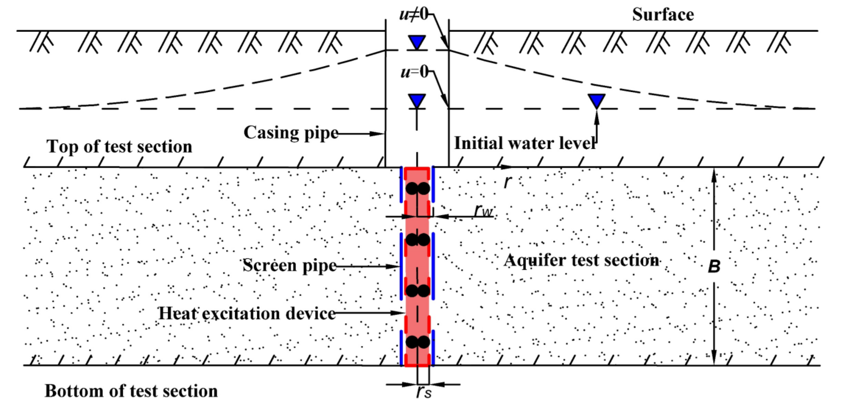
2.1. Establishment of Mathematical Model

The thermal transfer equation for the thermal convection-dispersion in the aquifer under radial flow conditions is as follows [40]:

$${\left(\rho c\right)}_{fs}\frac{\partial T}{\partial t}=\frac{1}{r}\frac{\partial }{\partial r}\left[r\lambda \left(r\right)\frac{\partial T}{\partial r}\right]-{\left(\rho c\right)}_{f}u\frac{\partial T}{\partial r}$$

(1)

According to the principle of heat conservation, the change of heat at the test section in the test well is equal to the change of heat at the aquifer $r=r_w$:

$${\left(\rho c\right)}_f\pi r_s^2\frac{d{T}_{*}}{dt}=2\pi r_w\lambda {\left.\frac{dT}{dr}\right|}_{r=r_w}$$

(2)

The initial conditions are as follows:

$${\left.T\left(r,t\right)\right|}_{t=0}=0,r>r_w$$

(3)

$$T_{*}\left(0\right)=T_0$$

(4)

The boundary conditions are as follows:

$${\left.T\left(r,t\right)\right|}_{r\to \infty }=0, t>0$$

(5)

$$T_{*}\left(t\right)=T\left(r_w,t\right),t>0$$

(6)

Among them, $T$ is the temperature $\left(\theta \right)$; $T\left(r_w,t\right)$ is the value of temperature change $\left(\theta \right)$ at the well wall of the test well at time $t$; $T\left(r,t\right)$ indicates the value of temperature change at any moment $t$ in the aquifer at a distance $r$ from the well center $\left(\theta \right)$; $T_{*}\left(t\right)$ is the value of temperature change $\left(\theta \right)$ of the test section in the test well at time $t$; $r$ is the radial distance from a point in the aquifer to the center of the test well $\left(L\right)$; $r_w$ is the radius of the test well $\left(L\right)$; $r_s$ is the radius of the cylindrical excitation device of the test well $\left(L\right)$; $t$ is time $\left(T\right)$; $\lambda \left(r\right)$ is the effective thermal conductivity of the aquifer $\left(LM{T}^{-3}{\theta }^{-1}\right)$; ${\left(\rho c\right)}_f$ is the groundwater heat capacity $\left(M{L}^{-1}{T}^{-2}{\theta }^{-1}\right)$; ${\left(\rho c\right)}_{fs}$ is the heat capacity of the aquifer $\left(M{L}^{-1}{T}^{-2}{\theta }^{-1}\right)$; $T_0$ is the initial temperature change value $\left(\theta \right)$; $u=\frac{Q}{2\pi Bnr}$ is the actual groundwater flow rate in the aquifer $\left(L{T}^{-1}\right)$; $B$ is the aquifer thickness $\left(L\right)$; $Q$ is the water injection flow rate $\left(L^3{T}^{-1}\right)$; $n$ is the aquifer porosity.

When $u=0$, no groundwater flow occurs in the aquifer and Equation (1) is converted to the heat conduction equation:

$${\left(\rho c\right)}_{fs}\frac{\partial T}{\partial t}=\frac{1}{r}\frac{\partial }{\partial r}\left[r\lambda \left(r\right)\frac{\partial T}{\partial r}\right]$$

(7)

Therefore, in order to solve the mathematical model, it is necessary to transform the above equations and the definite solution conditions into a dimensionless form by dimensionless factors and parametric variables, and then to perform Laplace transformations on them in turn.

2.2. Model Solution

2.2.1. Solution of the Theoretical Model When u = 0

Set the dimensionless factor: $T_D=\frac{T}{T_0}$, $\delta =\frac{r}{r_w}$, ${\delta }_s=\frac{r_s}{r_w}$, ${\delta }_w=\frac{r_w}{r_w}=1$, $\tau =\frac{\lambda t}{{\left(\rho c\right)}_{fs}{r}_w^2}$, $\gamma =\frac{{\left(\rho c\right)}_f{r}_s^2}{2{\left(\rho c\right)}_{fs}{r}_w^2}$, $\alpha =\frac{{\left(\rho c\right)}_f}{{\left(\rho c\right)}_{fs}}$.

Equation (7) is made dimensionless, giving:

$$\frac{\partial T_D}{\partial \tau }=\frac{{\partial }^2{T}_D}{{\partial }^2\delta }+\frac{1}{\delta }\frac{\partial T_D}{\partial \delta }$$

(8)

Equations (2)–(6) are made dimensionless in turn, giving:

$$\gamma \frac{d{T}_{*D}}{d\tau }=\frac{d{T}_D}{d\delta }$$

(9)

$$T_D\left(\delta ,0\right)=0,0<\delta <\infty , \tau =0$$

(10)

$$T_{*D}\left(0\right)=T_D,\delta =1, \tau =0$$

(11)

$$T_D\left(\delta ,\tau \right)=0,\delta \to \infty ,\tau >0$$

(12)

$$T_{*D}\left(\tau \right)=T_D\left(\delta ,\tau \right),\delta =1,\tau >0$$

(13)

Making Laplace transformations [41] on the parameters $\tau$ of Equation (8), Equation (8) is transformed into:

$$\frac{{\partial }^2\overline{T_D}}{\partial {\delta }^2}+\frac{1}{\delta }\frac{\partial \overline{T_D}}{\partial \delta }-p\overline{T_D}=0$$

(14)

Making Laplace transformations on the parameters $\tau$ of Equation (2), Equation (2) is transformed into:

$$\gamma \left(p\overline{T_{*D}}-1\right)=\frac{\partial \overline{T_D}\left(1,p\right)}{\partial \delta }$$

(15)

The Equations (3), (5), and (6) are converted by Laplace transformation to:

$$\overline{T_D}\left(\delta ,0\right)=0,\delta >0$$

(16)

$$\overline{T_D}\left(\infty ,p\right)=0,p>0$$

(17)

$$\overline{T_{*D}}\left(p\right)=\overline{T_D}\left(1,p\right)$$

(18)

Among them, $\overline{T_{*D}}$ is the image function of the Laplace transform of $T_{*D}$; $\overline{T_D}$ is the image function of the Laplace transform of $T_D$; $T_{*D}$ is the ratio of temperature variation in the test well; $T_D=\frac{T}{T_0}$ is the ratio of temperature variation in the aquifer; $\delta =\frac{r}{r_w}$ is the ratio of the radial distance from the test well center to the test well radius; ${\delta }_s=\frac{r_s}{r_w}$ is the ratio of the radius of the cylindrical excitation device in the test well to the test well; ${\delta }_w=1$; $p$ is the Laplace transform complex variable; $\tau =\frac{\lambda t}{{\left(\rho c\right)}_{fs}{r}_w^2}$ is the dimensionless time; $\gamma =\frac{{\left(\rho c\right)}_f{r}_s^2}{2{\left(\rho c\right)}_{fs}{r}_w^2}$ is the dimensionless parameter related to the inherent properties of the aquifer and the structure of the test well; $\alpha =\frac{{\left(\rho c\right)}_f}{{\left(\rho c\right)}_{fs}}$ is the ratio of the water heat capacity to the heat capacity of the aquifer.

According to the properties of the order n modified Bessel function [41]:

$$\frac{d^{2}y}{d{x}^2}+\frac{1}{x}\frac{dy}{dx}-\frac{1}{x^2}\left(x^2{\beta }^2+n^2\right)y=0$$

(19)

The general solution is:

$$y=C_1{K}_n\left(\beta x\right)+C_2{I}_n\left(\beta x\right)$$

(20)

where $I_n\left(x\right)$ and $K_n\left(x\right)$ are the first and second type of modified Bessel functions, respectively; when $n=0$, the solution of Equation (14) is:

$$\overline{T_D}\left(\delta ,p\right)=C_1{K}_0\left(\sqrt{p}\delta \right)+C_2{I}_0\left(\sqrt{p}\delta \right)$$

(21)

Based on the properties of Equation (17) after dimensionless change:

$$\underset{ \delta \to \infty }{ lim}\overline{T_D}\left(\delta ,p\right)=0$$

(22)

Because the first type of modified Bessel function $I_0\left(x\right)$ is an exponentially growing function with the property that $I_0\left(x\right)\to \infty$ as $x\to \infty$, it follows that $C_2=0$ in Equation (21), so the solution of Equation (14) is converted to:

$$\overline{T_D}\left(\delta ,p\right)=C_1{K}_0\left(\sqrt{p}\delta \right)$$

(23)

According to the properties of the order 0 modified Bessel function:

$$\frac{d}{dx}{K}_0\left(x\right)=-K_1\left(x\right)$$

(24)

$$\frac{d}{dx}{I}_0\left(x\right)=I_1\left(x\right)$$

(25)

Substituting Equation (23) into Equations (15) and (18), giving:

$$\gamma \left(p{C}_1{K}_0\left(\sqrt{p}\right)-1\right)=-C_1\sqrt{p}{K}_1\left(\sqrt{p}\right)$$

(26)

By Equation (26), giving:

$$C_1=\frac{\gamma }{\gamma p{K}_0\left(\sqrt{p}\right)+\sqrt{p}{K}_1\left(\sqrt{p}\right)}$$

(27)

Therefore, when $u=0$, the analytical solution of the theoretical model in Laplace space can be obtained as:

$$\overline{T_D}\left(\delta ,p\right)=\frac{\gamma K_0\left(\sqrt{p}\delta \right)}{\gamma p{K}_0\left(\sqrt{p}\right)+\sqrt{p}{K}_1\left(\sqrt{p}\right)}$$

(28)

$$\overline{T_{*D}}\left(p\right)=\frac{\gamma K_0\left(\sqrt{p}\right)}{\gamma p{K}_0\left(\sqrt{p}\right)+\sqrt{p}{K}_1\left(\sqrt{p}\right)}$$

(29)

Equation (29) is the final solution derived in the Laplace transform domain under the condition of $u=0$. However, in order to apply this solution in practical experiments, it is necessary to perform an inverse Laplace transform on Equation (29). Among the Laplace numerical inversion methods, the Stehfest (1970) method [42] is widely used for its simplicity and short computation time:

$$f\left(t\right)=\frac{\ln 2}{t}{\displaystyle \sum }_{i=1}^N{V}_{i}F\left(\frac{\ln 2}{t}i\right)$$

(30)

where $f\left(t\right)$ is the image primitive function in real space; $F\left(s\right)$ is the image function in Laplace space; $N$ is the number of summation terms:

$$V_i={\left(-1\right)}^{\frac{N}{2}+i}{\displaystyle \sum }_{k=\left[\frac{i+1}{2}\right]}^{Min\left(i,\frac{N}{2}\right)}\frac{k^{\frac{N}{2}+1}\left(2k\right)!}{\left(\frac{N}{2}-k\right)!k!\left(k-1\right)!\left(i-k\right)!\left(2k-i\right)!}$$

(31)

Substituting Equation (29) into Equation (30) for the Laplace inversion, giving:

$$T_{*D}\left(\tau \right)=\frac{\ln 2}{\tau }{\displaystyle \sum }_{i=1}^N{V}_i\overline{T_{*D}}\left(\frac{\ln 2}{\tau }i\right)$$

(32)

In summary:

$$T_{*D}=f\left(\alpha ,\gamma ,\tau \right)$$

(33)

It can be seen that there are three dimensionless parameters $\alpha , \gamma$, and $\tau$ that control the dimensionless temperature variation $T_{*D}$ in the test well in the theoretical model of the slug heat test when $u=0$.

2.2.2. Solution of the Theoretical Model When u ≠ 0

Equation (1) is made dimensionless, giving:

$$\frac{\partial T_D}{\partial \tau }=\frac{{\partial }^2{T}_D}{\partial {\delta }^2}+\frac{\beta }{\delta }\frac{\partial T_D}{\partial \delta }$$

(34)

Making Laplace transformations on the dimensionless factor $\tau$ of Equation (34), Equation (34) is transformed into:

$$\frac{{\partial }^2\overline{T_D}}{\partial {\delta }^2}+\frac{\beta }{\delta }\frac{\partial \overline{T_D}}{\partial \delta }-p\overline{T_D}=0$$

(35)

where $\beta =\frac{\lambda -{\left(\rho c\right)}_{f}ur}{\lambda }=\frac{\lambda -{\left(\rho c\right)}_f\frac{Q}{2\pi Bn}}{\lambda }=1-\frac{{\left(\rho c\right)}_{fs}\alpha \frac{Q}{2\pi Bn}}{\lambda }=1-\frac{\alpha \frac{Q}{2\pi Bn}}{\eta }$; Among them, $\eta =\frac{\lambda }{{\left(\rho c\right)}_{fs}}$ is the thermal diffusivity $\left(L^2{T}^{-1}\right)$, which reflects the rapidity of the thermal conductivity of the aquifer;$\beta$ is a parameter related to the aquifer properties and groundwater flow rate.

In order to make Equation (35) applicable to the order n modified Bessel Equation (19), the following transformation of Equation (35) is required $y=\overline{T_D}$ and $x=\delta$. Then, Equation (35) is transformed as follows:

$$\mathrm{x}{y}^{″}+\beta y^{\prime }-pxy=0$$

(36)

Set $y=x^{-m}·u,m=\frac{\beta -1}{2}$, giving:

$$y^{\prime }=x^{-m}{u}^{\prime }-m{x}^{-m-1}u$$

(37)

$$y^{″}=x^{-m}{u}^{″}-2m{x}^{-m-1}{u}^{\prime }+m\left(m+1\right)x^{-m-2}u$$

(38)

Substituting Equation (37) and Equation (38) into Equation (36) gives:

$$u^{″}+\frac{1}{x}{u}^{\prime }-\frac{1}{x^2}(x^{2}p+m^2)u=0$$

(39)

Therefore, according to the solution of the order n modified Bessel equation, giving:

$$u=C_1{K}_n\left(\sqrt{p}x\right)+C_2{I}_n\left(\sqrt{p}x\right)$$

(40)

$$\mathrm{y}=x^{-m}·\left[C_1{K}_n\left(\sqrt{p}x\right)+C_2{I}_n\left(\sqrt{p}x\right)\right]$$

(41)

When $n=0$, it is obtained that:

$$\overline{T_D}\left(\delta ,p\right)={\delta }^{\frac{1-\beta }{2}}\left[C_1{K}_0\left(\sqrt{p}\delta \right)+C_2{I}_0\left(\sqrt{p}\delta \right)\right]$$

(42)

According to the definite solution condition and the first type of modified Bessel function $I_0\left(x\right)$ with the following property: $I_0\left(x\right)\to \infty$ when $x\to \infty$, it is obtained that $C_2=0$, Equation (42) is transformed to:

$$\overline{T_D}\left(\delta ,p\right)={\delta }^{\frac{1-\beta }{2}}{C}_1{K}_0\left(\sqrt{p}\delta \right)$$

(43)

Substituting Equation (43) and Equation (18) into Equation (15), giving:

$$\mathsf{\gamma }\left[\mathrm{p}{C}_1{K}_0\left(\sqrt{p}\right)-1\right]=\frac{1-\beta }{2}{C}_1{K}_0\left(\sqrt{p}\right)-C_1\sqrt{p}{K}_1\left(\sqrt{p}\right)$$

(44)

After sorting, we obtain:

$$C_1=\frac{\mathsf{\gamma }}{\left(\mathsf{\gamma }\mathrm{p}-\frac{1-\beta }{2}\right)K_0\left(\sqrt{p}\right)+\sqrt{p}{K}_1\left(\sqrt{p}\right)}$$

(45)

Therefore, when $u\ne 0$ in the aquifer, the analytical solution of the slug heat test theoretical model in Laplace space can be obtained as:

$$\overline{T_D}\left(\delta ,p\right)=\frac{\mathsf{\gamma }{\delta }^{\frac{1-\beta }{2}}{K}_0\left(\sqrt{p}\delta \right)}{\left(\mathsf{\gamma }\mathrm{p}-\frac{1-\beta }{2}\right)K_0\left(\sqrt{p}\right)+\sqrt{p}{K}_1\left(\sqrt{p}\right)}$$

(46)

$$\overline{T_{*D}}\left(p\right)=\frac{\mathsf{\gamma }{K}_0\left(\sqrt{p}\right)}{\left(\mathsf{\gamma }\mathrm{p}-\frac{1-\beta }{2}\right)K_0\left(\sqrt{p}\right)+\sqrt{p}{K}_1\left(\sqrt{p}\right)}$$

(47)

When performing numerical inversion of the Laplace transform domain, the Stehfest algorithm is prone to numerical dispersion in the case of convective dominance of large groundwater flow rate, so another Talbot algorithm [43,44] is considered, which takes into account the complex variable domain and its accuracy is much greater than that of the Stehfest algorithm and is more stable:

$$f\left(t\right)=\frac{p}{N}\left(\frac{1}{2}F\left(p\right)e^{pt}+{\displaystyle \sum }_{k=1}^{N-1}Re\left[e^{ts\left({\theta }_k\right)}F\left(s\left({\theta }_k\right)\left(1+\sigma \left({\theta }_k\right)\right)\right)\right]\right)$$

(48)

where $f\left(t\right)$ is the image primitive function in real space; $F\left(p\right)$ is the image function in Laplace space; $p=\frac{2N}{5t}$;$s\left(\theta \right)=p\theta \left(cot\theta +i\right)$;${\theta }_k=\frac{k\pi }{N}$;$\sigma \left(\theta \right)=\theta +\left(\theta cot\theta -1\right)cot\theta$.

Substituting Equation (47) into Equation (48) for the Laplace inverse transform gives:

$$T_{*D}=f\left(\alpha ,\beta ,\gamma ,\tau \right)$$

(49)

It can be seen that there are four dimensionless parameters, $\alpha ,\beta ,\gamma ,$ and $\tau$, that control the dimensionless temperature variation $T_{*D}$ in the test well in the theoretical model of the slug heat test when $u\ne 0$.

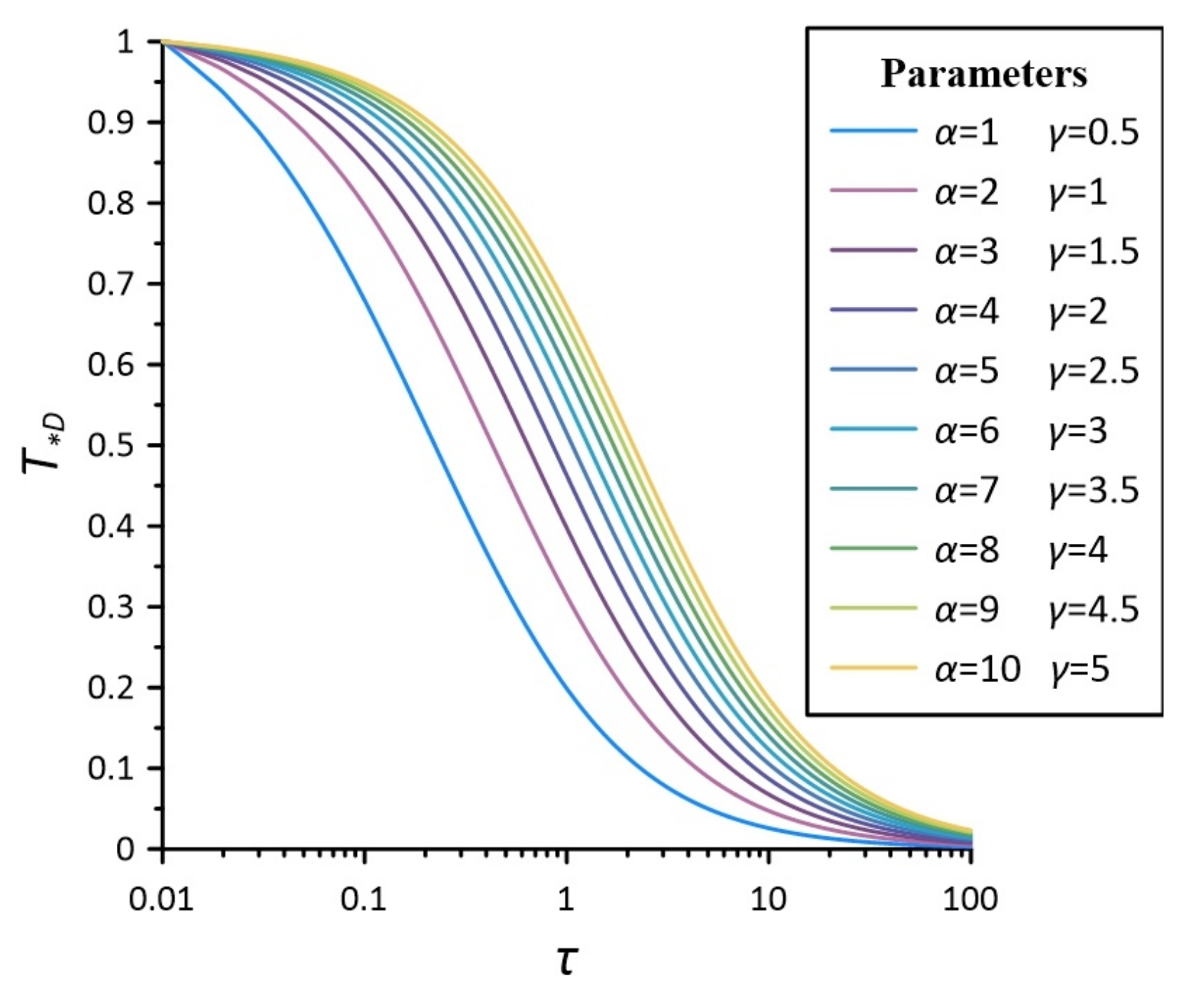
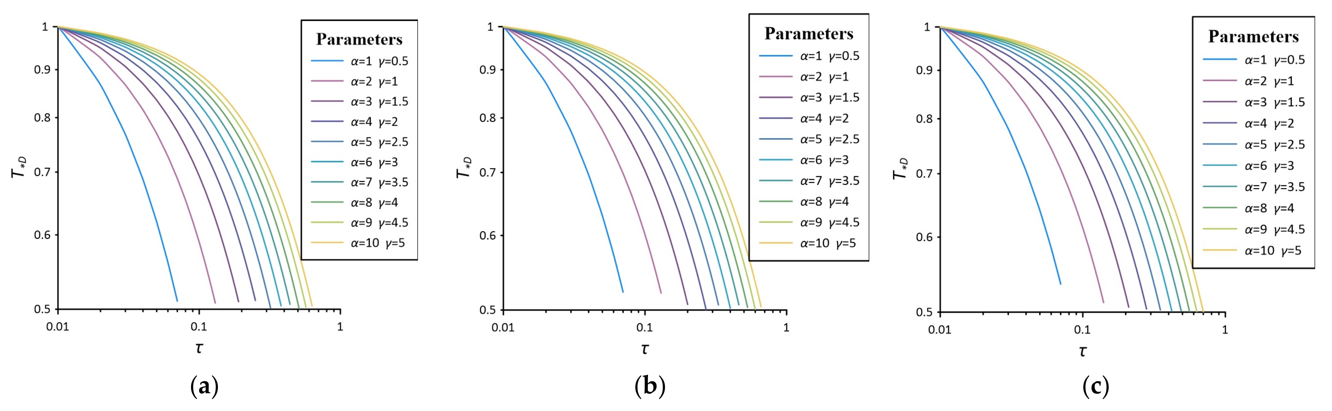
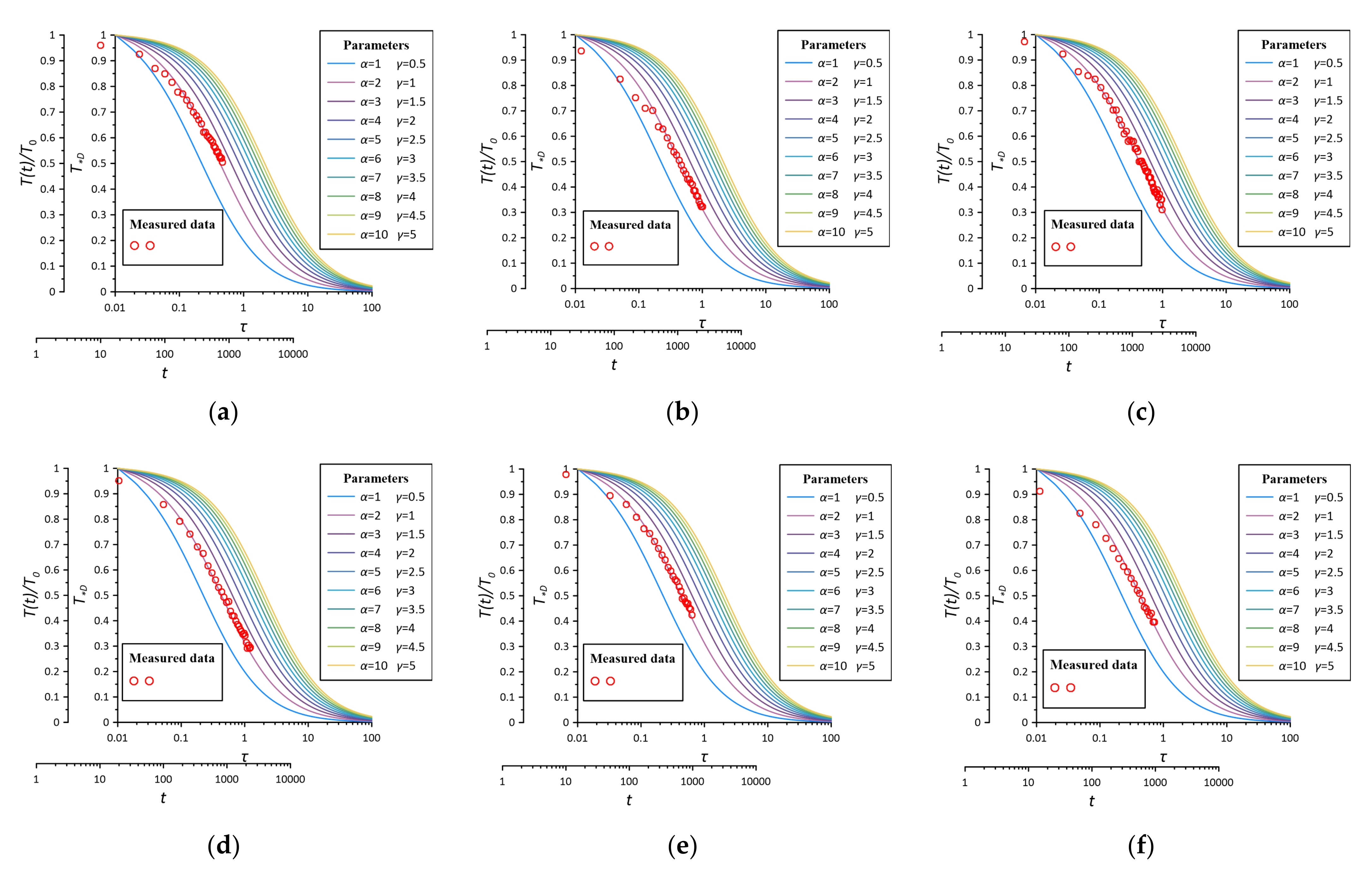
2.2.3. Standard Curve Plotting and Parameter Calculation Method

In the case of $u=0$, according to Equation (33), where $\alpha$ is taken in the range of 1 to 10, dimensionless time $\tau$ is taken in the range of 0.01 to 100, and $N$ is taken as 8. The Stehfest algorithm is chosen to establish a set of standard curves of dimensionless temperature variation $T_{*D}$ with dimensionless time $\tau$ with respect to $\alpha ,\gamma$ parameters in the case of $u=0$, as shown in Figure 2.

In the case of $u\ne 0$, according to Equation (49), where $\alpha$ is taken in the range of 1 to 10, $\beta$ is taken in the range of −1 to 0 according to aquifer properties and seepage conditions, the dimensionless time $\tau$ is taken in the range of 0.01 to 1, and $N$ is taken as 16. The Tolbot algorithm is chosen to establish a set of dimensionless temperature variation $T_{*D}$, with dimensionless time $\tau$ with respect to $\alpha ,\gamma ,\beta$ parameters in the case of $u\ne 0$, as shown in Figure 3. According to the definition of the $\beta$ parameter, the corresponding flow rate $u$ increases as the $\beta$ parameter decreases, and the $\beta$ value has little effect on the curve shape and curvature in this test flow rate. Therefore, the standard curve of intermediate segment $\beta =-0.5$ is chosen for data fitting.

The temperature of the test section in the test well changes instantaneously by the slug heat test, the temperature change of the test section in the test well with time is recoded, the temperature difference ratio $\frac{Tt}{T_0}$ and the test time $t$ at the test section in the test well under different seepage conditions are obtained and the measured relationship curve of $\frac{T\left(t\right)}{T_0}$ and $t$ is plotted. Among them, the axis of time $t$ is taken as a logarithmic axis in the case of $u=0$, and the temperature difference ratio and time are both taken as logarithmic axes in the case of $u\ne 0$.

The steps to obtain the thermal conductivity of the aquifer from the slug heat test and derive the other thermal property parameters by the formula are as follows: (i) The measured curves in the case of $u=0$ and $u\ne 0$ respectively correspond to the standard curves under the corresponding conditions in the plotting software, and placed respectively in semi-logarithmic and double logarithmic coordinates with the same modulus. Fix the vertical coordinates at the same height and translate the horizontal coordinates until the two curves overlap. (ii) Take any matching point and record the corresponding coordinate values of the matching point:$\left[t\right]$,$\left[\tau \right]$,$\left[\alpha \right]$, where, in the case of $u\ne 0$, it is also necessary to record the value of the corresponding standard curve: [$\beta$]. (iii) The heat capacity of water ${\left(\rho c\right)}_f$, the thermal conductivity of water ${\lambda }_f$ and the radius of test well $r_w$ are known, according to the standard curve in the case of $u=0$, based on ${\left(\rho c\right)}_{fs}=\frac{{\left(\rho c\right)}_f}{\left[\alpha \right]}$ to calculate the heat capacity of the aquifer ${\left(\rho c\right)}_{fs}$, and then based on ${\lambda }_{*}=\frac{\left[\tau \right]r_w^2{\left(\rho c\right)}_f}{\left[t\right]\left[\alpha \right]}$ to calculate the stagnant thermal conductivity of aquifer ${\lambda }_{*}$. (iv) According to the standard curve in the case of $u\ne 0$, based on $\lambda =\frac{\left[\tau \right]r_w^2{\left(\rho c\right)}_f}{\left[t\right]\left[\alpha \right]}$, the effective thermal conductivity of the aquifer $\lambda$ can be obtained, and at the same time, the thermal diffusivity of the aquifer can be obtained according to $\eta =\frac{\lambda }{{\left(\rho c\right)}_{fs}}$. (v) The effective thermal conductivity of the aquifer $\lambda$ in the thermal convection-dispersion model is composed of two parts: the stagnant thermal conductivity ${\lambda }_{*}$ when the groundwater is not flowing and the thermal mechanical dispersion coefficient ${\lambda }_v$; therefore, the thermal mechanical dispersion coefficient of the aquifer ${\lambda }_v$ can be obtained based on ${\lambda }_v=\lambda -{\lambda }_{*}$. The thermal mechanical dispersion coefficient ${\lambda }_v$ is closely related to the flow rate of the aquifer, and the longitudinal thermal mechanical dispersion coefficient ${\lambda }_v$ is considered to be proportional to the flow rate $u$, and therefore, it can be expressed as ${\lambda }_v=a_x{\left(\rho c\right)}_{f}u$, and the thermal dispersive degree $a_x$ is derived based on $a_x=\frac{\lambda -{\lambda }_{*}}{{\left(\rho c\right)}_{f}u}$. In addition, the porosity $n$ is known based on the indoor geotechnical test data, based on ${\left(\rho c\right)}_{fs}=n{\left(\rho c\right)}_f+\left(1-n\right){\left(\rho c\right)}_s$ to calculate the heat capacity of the rock-soil skeleton ${\left(\rho c\right)}_s$, and then based on ${\lambda }_{*}={\left(\rho c\right)}_{fs}\left[\frac{n{\lambda }_f}{{\left(\rho c\right)}_f}+\frac{(1-n){\lambda }_s}{{\left(\rho c\right)}_s}\right]$ to calculate the thermal conductivity of rock-soil skeleton ${\lambda }_s$.

Therefore, the thermal property parameters such as stagnant thermal conductivity and effective thermal conductivity of the aquifer can be obtained by slug heat tests in the cases of $u=0$ and $u\ne 0$. At the same time, according to stagnant thermal conductivity and effective thermal conductivity of the aquifer, not only can the thermal property parameters such as the thermal conductivity of the rock-soil skeleton be deduced, but also the transfer law of heat in the aquifer can be explored.

3. Construction of an Indoor Test Platform and Slug Heat Test

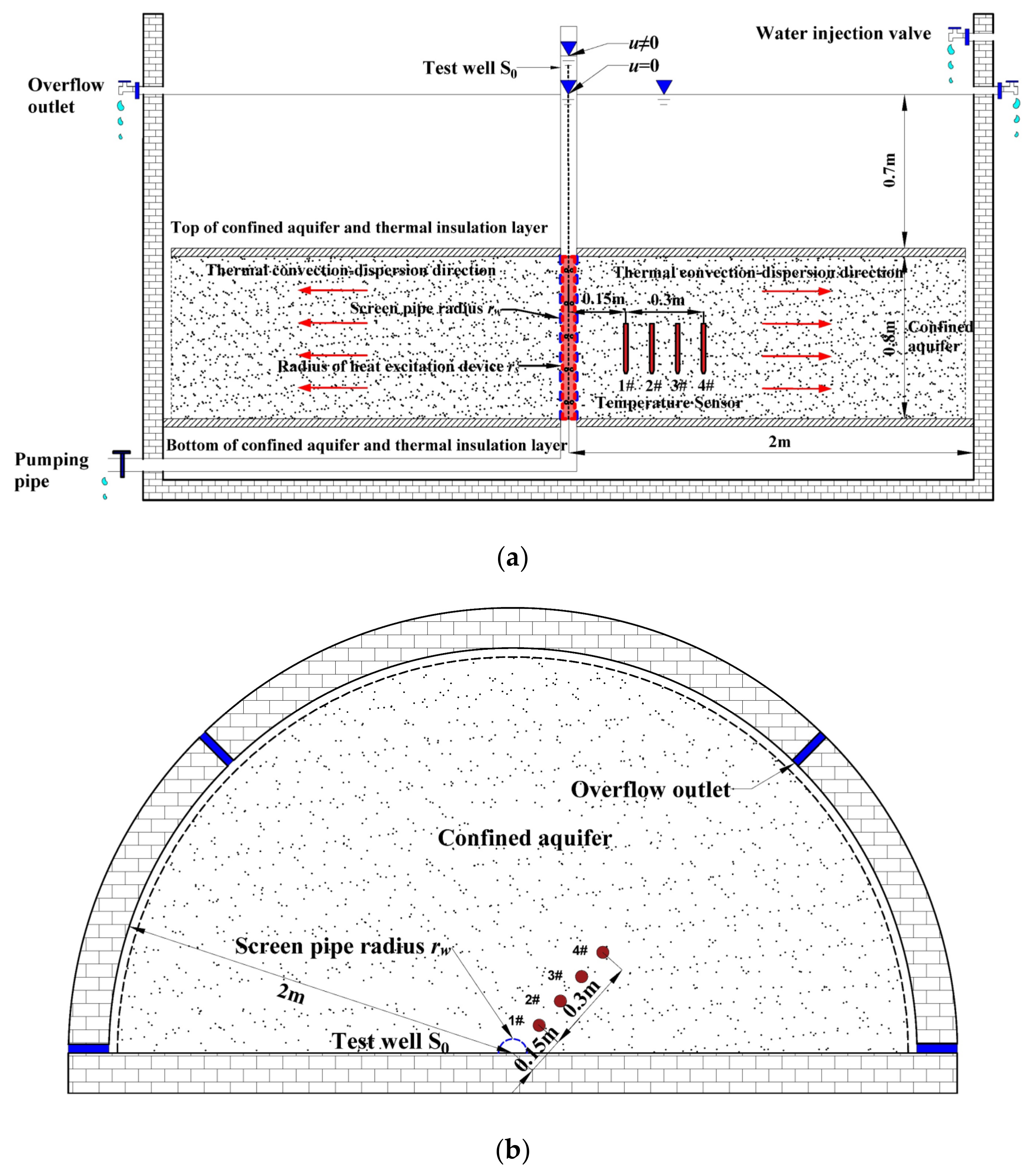
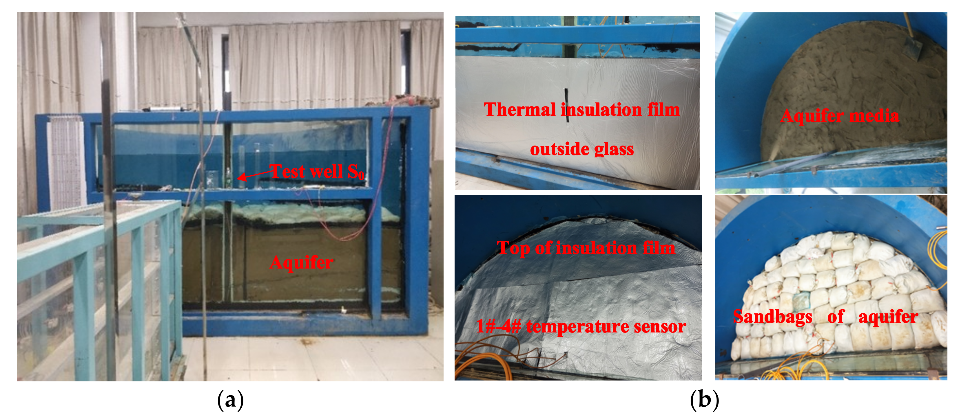
In order to verify the accuracy and applicability of the derived slug heat test theoretical model, parameter calculation method and slug heat test method, the constructed semi-cylindrical sand tank was used to simulate the confined aquifer system and carry out the research of the slug heat test. The test data were fitted to the standard curve of the slug heat test theoretical model by the curve fitting method, and the thermal property parameters of aquifers and rock-soil skeletons were obtained and compared with the relevant empirical values for analysis.

3.1. Test Platform

The system consists of three parts: model frame, confined aquifer system and observation system. Based on the consideration of saving space and satisfying the test conditions, according to the thermal radial convection-dispersion theory and the principle of axial symmetry, the test platform is designed as a semi-cylindrical sand tank as shown in Figure 4. The test well is set in the center of the semi-cylindrical section, and the overflow outlet is set on one side of the semi-cylindrical arc to ensure that the boundary is a constant water head boundary during the test, and observation points are arranged in the radial direction of the model to obtain water level and temperature data.

The model is a semi-cylindrical steel frame with a height of 2.2 m and a radius of 2 m. A semi-cylindrical test well with an inner radius of 4 cm is set at the center of the front of the platform, a support frame is set at the side and bottom, and a pumping pipe is set at the bottom. A glass transparent window is built on the front side for easy observation of the test process, as shown in Figure 5a. The test platform simulates a confined aquifer, with a thickness of 0.8 m and medium-fine sand with particle size of 0.25 mm to 0.50 mm. The top and bottom of the confined aquifer are covered with plastic film and thermal insulation film for waterproof and thermal insulation treatment. Sandbags are laid on the top to apply pressure, and groundwater is supplied from the side of the confined aquifer. The aquifer temperature observation device is mainly composed of test well S₀ and pt100 type temperature sensors of $1\#$, $2\#$, $3\#$ and $4\#$ pre-buried in the aquifer at different distances from the test well, and the temperature data are monitored and uploaded to the computer terminal for data processing, as shown in Figure 5b. Four overflow outlets with a radius of 2 cm are set at a height of 1.5 m from the bottom of the confined aquifer to meet the requirements of constant water head. The physical picture of the test platform is shown in Figure 5.

3.2. Test Instrument and Method

The slug heat test is analogous to the slug test, which is to change the temperature of the test section in the test well instantaneously, record the temperature change of the test section in the test well with time, study the temperature change law and then obtain the relevant thermal property parameters of the aquifers and rock-soil skeletons. The test data acquisition equipment consist of a Pt100 thermal resistance temperature sensor. The Pt100 sensor is connected with an external digital display instrument to monitor the temperature and computer system through the converter to monitor and record the temperature change data in the test well in real time. When $u=0$, the hot water of a certain known temperature is instantaneously injected into the test section through the excitation device, and the water level in the test well is kept consistent with the water level of the aquifer; when $u\ne 0$, the hot water of a certain known temperature is instantaneously injected into the test section through the excitation device, while the water head in the test well is kept at a certain higher height than the initial water level of the aquifer to achieve different seepage conditions of the slug heat test.

The indoor experimental research was divided into four seepage conditions: $u=0$, $u$ of 9.30 × 10⁻³ cm/s, 6.82 × 10⁻³ cm/s and 4.34 × 10⁻³ cm/s, respectively, and three groups of slug heat tests with different temperature excitation strengths under each seepage condition are carried out. The measured temperature data of the test well are taken as the data of calculation parameters, and two sets of parallel tests were conducted for each group of tests, with a total of twenty-four groups. The test platform and the values of the calculated parameters are shown in

Table 1. The test platform parameters and the calculated parameters values.

Parameters	Value	Unit
Aquifer thickness $B$	0.8	$\mathrm{m}$
Medium particle size $d$	0.25–0.50	$\mathrm{mm}$
Aquifer porosity $n$	0.33	/
heat capacity of water ${\left(\rho c\right)}_f$	4.18 × 106	J/(m3·K)
thermal conductivity of water ${\lambda }_f$	0.62	W/(m·°C)
Test well radius $r_w$	4	c$\mathrm{m}$
Radius of heat excitation device $r_s$	4	$\mathrm{cm}$
Flow Rate $u$	4.34–9.30 × 10−3	cm/s

.

4. Analysis of the Slug Heat Test Results

The standard curves of different seepage conditions are obtained based on the theoretical model of the slug heat test, and the measured temperature data and standard curves under different seepage conditions are fitted to obtain the stagnant thermal conductivity of aquifer, heat capacity of aquifer, effective thermal conductivity of aquifer, thermal mechanical dispersion coefficient, longitudinal thermal dispersive degree and thermal diffusivity of the aquifer. At the same time, the heat capacity and thermal conductivity of the rock-soil skeleton can also be calculated. By comparing and analyzing with the empirical values, we can verify the accuracy and feasibility of the theoretical model and parameter calculation method of the slug heat test and explore the heat transfer law in the aquifer.

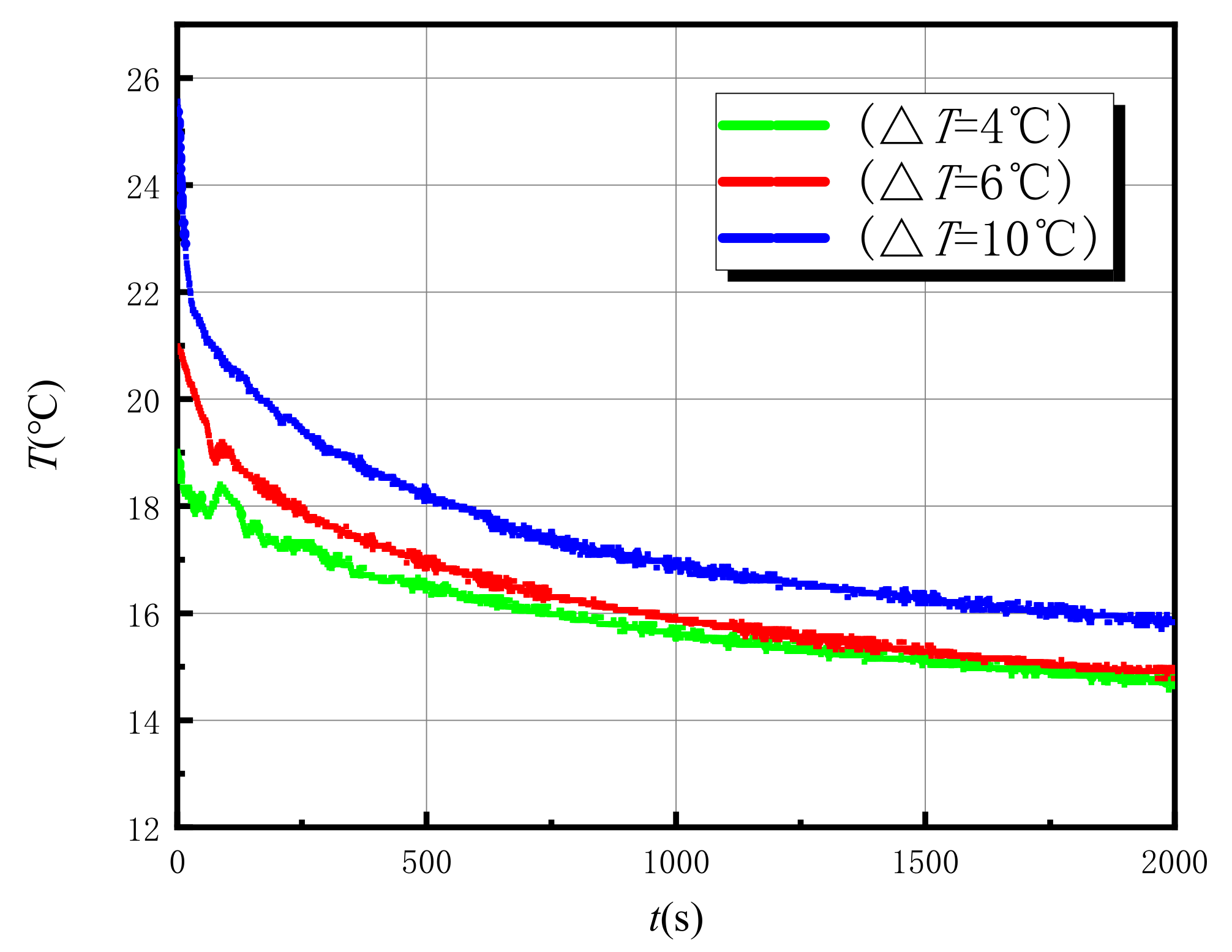
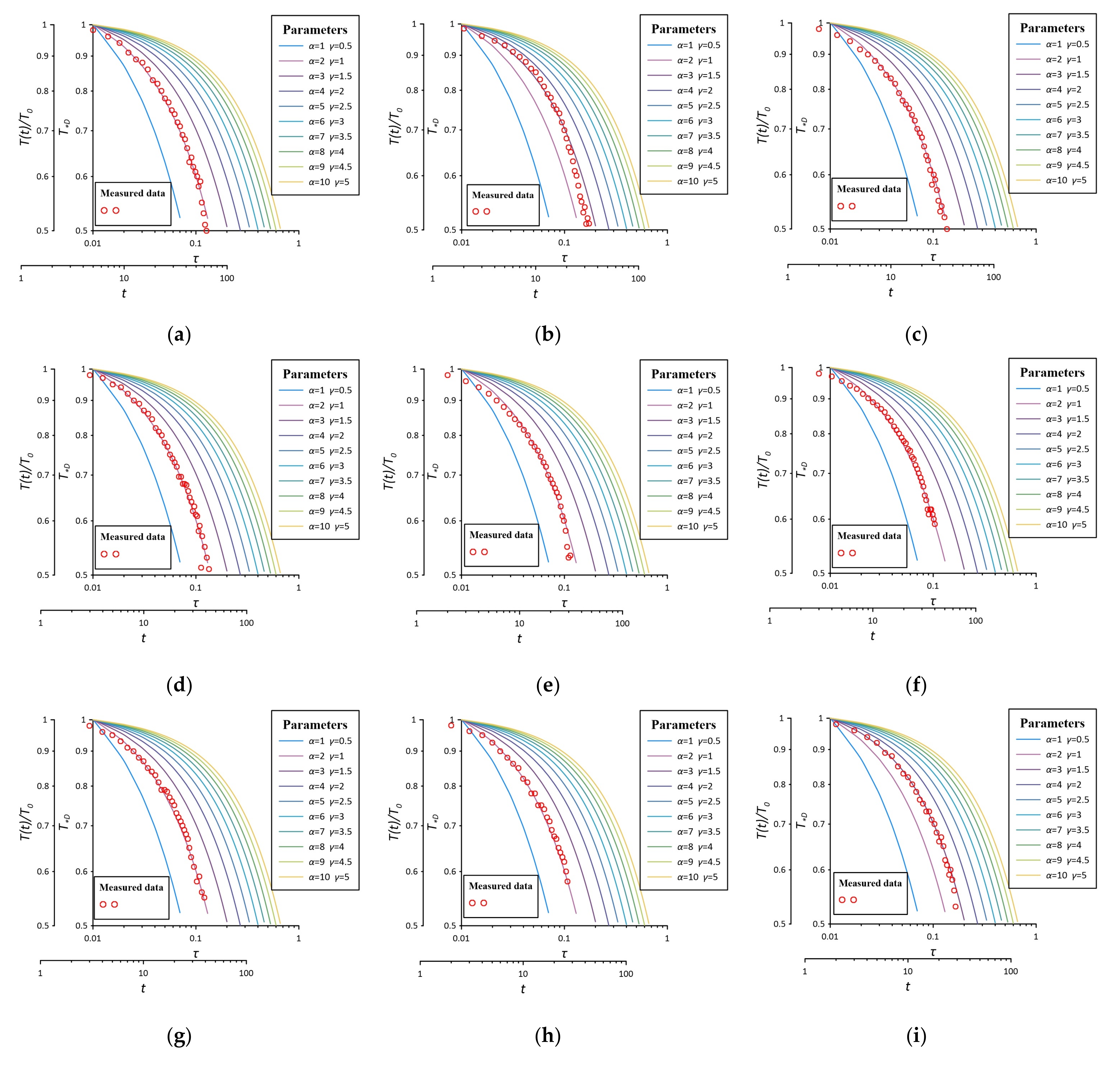
4.1. Analysis of Slug Heat Test Results in the Case of u = 0

In the case of u = 0, three different excitation strengths are used (the temperature difference is $\Delta T=4 °\mathrm{C}, \Delta T=6 °\mathrm{C},\Delta T=10 °\mathrm{C}$), and two groups of parallel experiments are carried out for each excitation strength, with a total of six groups. The theoretical model of the slug heat test is used for calculation and analysis. The temperature variation curve of the test well with time for different excitation strengths in the case of $u=0$ is shown in Figure 6. It can be seen that with the increase of the excitation temperature, the peak value of the curve also increases, and the time range of large change amplitude of the temperature is between 0–2000 s.

Plot measured curves of $\frac{T\left(t\right)}{T_0}-lgt$ semi-logarithmic coordinate in plotting software based on the measured test data of the dimensionless temperature change value $\frac{T\left(t\right)}{T_0}$ and time $t$ in the test well, and fit the standard curve in the case of $u=0$. The matching diagram of six groups of tests data are shown in Figure 7.

Take any matching point, record the corresponding coordinate value of the matching point $\left[\tau \right]$ and $\left[t\right]$, record the value $\left[\alpha \right]$ of the fitted standard curve, obtain the stagnant thermal conductivity of the aquifer according to ${\lambda }_{*}=\frac{\tau r_w^2{\left(\rho c\right)}_f}{t\alpha }$ and also obtain the heat capacity of the aquifer according to $\alpha =\frac{{\left(\rho c\right)}_f}{{\left(\rho c\right)}_{fs}}$; the calculation results are shown in

Table 2. Calculation results of the thermal property parameters of the aquifer by the slug heat test method in the case of $u=0$.

Test No.	$\mathsf{\alpha }$	Heat Capacity of Water ${\left(\mathit{\rho }\mathit{c}\right)}_{\mathit{f}}$ (J/(m3·K))	Heat Capacity of Aquifer ${\left(\mathit{\rho }\mathit{c}\right)}_{\mathit{f}\mathit{s}}$ (J/m3·K))	Stagnant Thermal Conductivity of Aquifer ${\mathit{\lambda }}_{*}$ (W/(m·°C))	Average value of ${\mathit{\lambda }}_{*}$ (W/(m·°C))
$w\left(\mathsf{\Delta }T=4 °\mathrm{C}\right)1$	2	4.18 × 106	2.09 × 106	1.67	1.5
$w\left(\mathsf{\Delta }T=4 °\mathrm{C}\right)2$	2		2.09 × 106	1.33
$w\left(\mathsf{\Delta }T=6 °\mathrm{C}\right)1$	2		2.09 × 106	1.15	1.46
$w\left(\mathsf{\Delta }T=6 °\mathrm{C}\right)2$	2		2.09 × 106	1.76
$w\left(\mathsf{\Delta }T=10 °\mathrm{C}\right)1$	2		2.09 × 106	1.97	2.10
$w\left(\mathsf{\Delta }T=10 °\mathrm{C}\right)2$	2		2.09 × 106	2.23
Average value of stagnant thermal conductivity					1.69

. Among them, the symbol $w$ indicates that the water flow state is not considered, $\mathsf{\Delta }T$ represents the temperature difference between the excitation temperature and the initial temperature of the aquifer and the number indicates test groups.

As can be seen from Table 2, the thermal conductivity and heat capacity of water are obtained based on empirical values, and the heat capacity of aquifer is obtained based on the fitting curve data $\alpha$. According to ${\left(\rho c\right)}_{fs}=n{\left(\rho c\right)}_f+\left(1-n\right){\left(\rho c\right)}_s$, the heat capacity of the rock-soil skeleton ${\left(\rho c\right)}_s$ is obtained. Meanwhile, according to ${\lambda }_{*}={\left(\rho c\right)}_{fs}\left[\frac{n{\lambda }_f}{{\left(\rho c\right)}_f}+\frac{(1-n){\lambda }_s}{{\left(\rho c\right)}_s}\right]$, the thermal conductivity of the rock-soil skeleton ${\lambda }_s$ is also obtained. The calculation results are shown in

Table 3. Calculation results of the thermal property parameters of the rock-soil skeleton.

Stagnant Thermal Conductivity of Aquifer ${\mathit{\lambda }}_{*}$ (W/(m·°C))	Thermal Conductivity of Water ${\mathit{\lambda }}_{\mathit{f}}$ (W/(m·°C))	Heat Capacity of Rock-Soil Skeleton ${\left(\mathit{\rho }\mathit{c}\right)}_{\mathit{s}}$ (J/(m3·K))	Thermal Conductivity of Rock-Soil Skeleton ${\mathit{\lambda }}_{\mathit{s}}$ (W/(m·°C))	Average Value of ${\mathit{\lambda }}_{\mathit{s}}$ (W/(m·°C))
1.5	0.62	1.06 × 106	1.06	1.2
1.46		1.06 × 106	1.03
2.10		1.06 × 106	1.51

.

The medium of indoors aquifer model is medium-fine sand with particle size in the range of 0.25 mm to 0.50 mm, and the aquifer porosity $n$ is $0.33$ according to the indoor geotechnical test. It can be seen from Table 3 that the average value of the thermal conductivity of the rock-soil skeleton is 1.2 W/(m·°C). The thermal conductivity of medium-fine sand is generally in the range of 1.0 to 5.0 W/(m·°C) according to literature and manuals [15], which is consistent with the results of this test. It can also prove the accuracy and feasibility of slug heat tests to determine the thermal property parameters of aquifers and rock-soil skeletons.

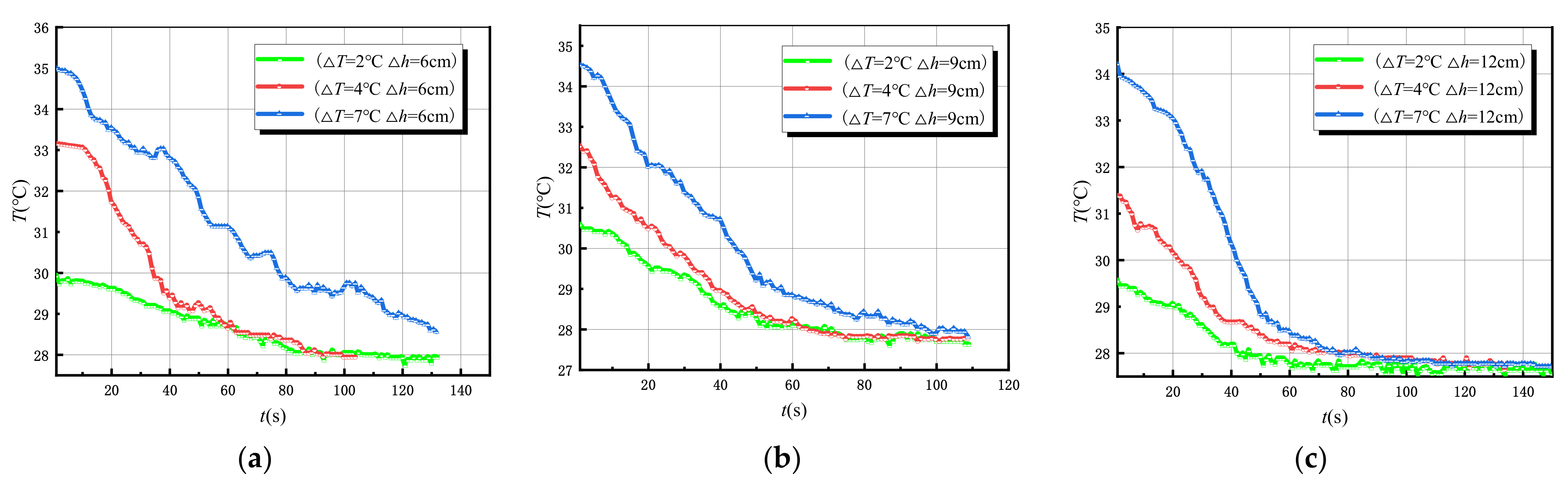
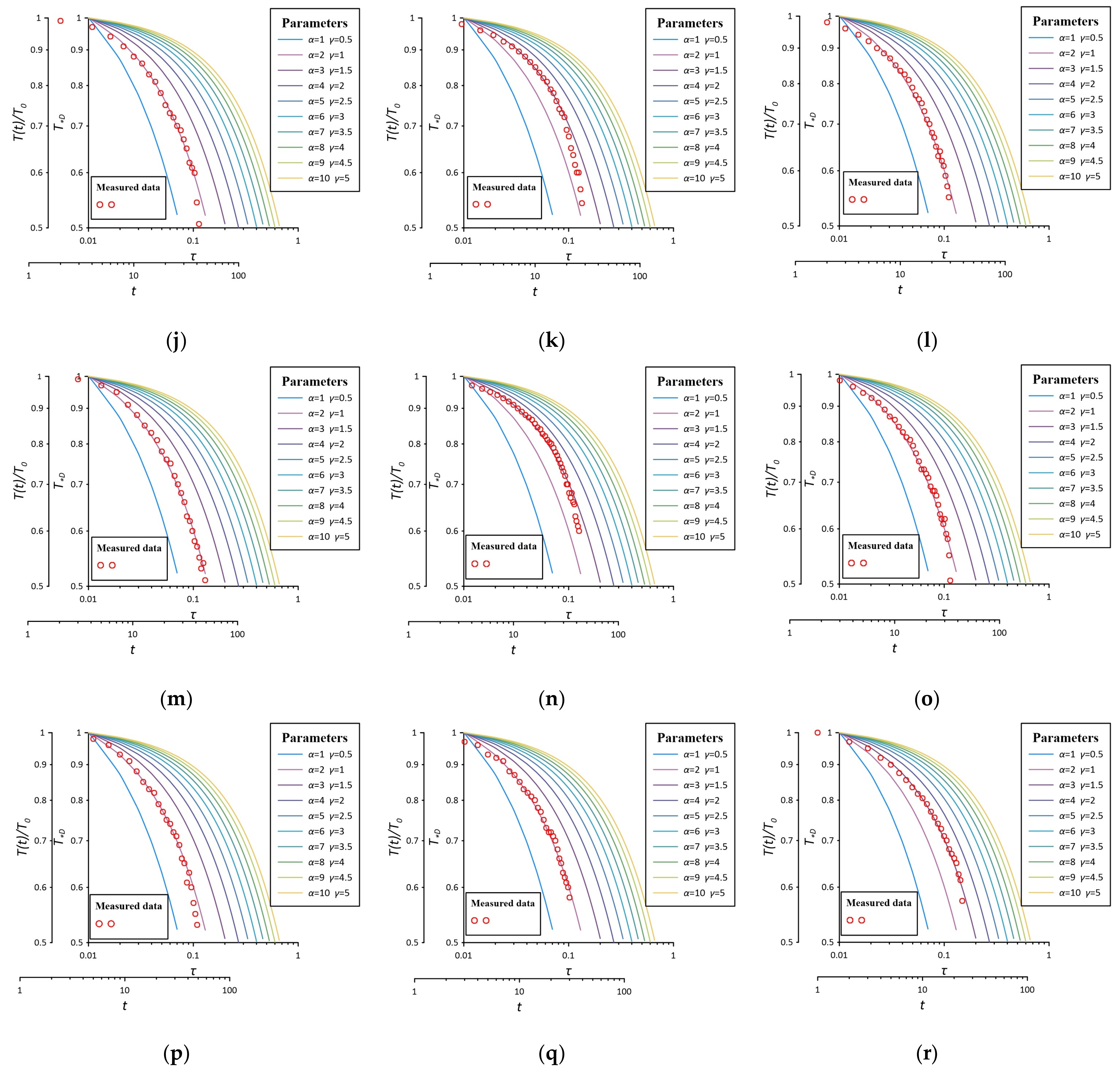
4.2. Analysis of Slug Heat Test Results in the Case of u ≠ 0

In the case of u ≠ 0, three different flow velocity states, namely, three different water head differences between the test well and the confined aquifer ($∆h=6 \mathrm{cm}, ∆h=9 \mathrm{cm}, ∆h=12 \mathrm{cm}$) and three different excitation strengths ($∆T=2 °\mathrm{C}, ∆T=4 °\mathrm{C}, ∆T=7 °\mathrm{C}$) are carried out by the slug heat test. Two groups of parallel experiments under each test condition are carried out, with a total of 18 groups. The measured temperature variation curves of the test well are shown in Figure 8. It can be intuitively seen that the time of temperature change in the case of $u\ne 0$ is mainly within 100 s after the injection of hot water, which is much shorter than that in the case of $u=0$, and the heat change is mainly completed by convection-dispersion. In addition, the change rate of temperature in the test well also increases with the increase of the flow rate.

Plot measured curves of $lg\frac{T\left(t\right)}{T_0}-lgt$ double logarithmic coordinate in plotting software based on the measured test data of the dimensionless temperature change value $\frac{T\left(t\right)}{T_0}$ and time $t$ in the test well, and fit the standard curve in the case of $u\ne 0$. The matching diagram of eighteen groups of slug heat tests are shown in Figure 9. In order to maintain the constant water head of the slug heat test, we continuously inject cold water into the test well; the cold water and heat source will have a mixing effect, resulting in a rapidly declining rate in the later stage of the curve. During matching, the front part of curve shall be used for fitting, because the mixing effect is not obvious in this time period. The heat is transferred in the aquifer through the inherent conduction and convection-dispersion in the case of $u\ne 0$.

Take any matching point, write down the corresponding coordinate value of the matching point $\left[\tau \right]$ and $\left[t\right]$, record the value $\left[\alpha \right]$ of the fitted standard curve, obtain the effective thermal conductivity of the aquifer according to $\lambda =\frac{\tau r_w^2{\left(\rho c\right)}_f}{t\alpha }$ and also obtain the heat capacity of the aquifer according to $\alpha =\frac{{\left(\rho c\right)}_f}{{\left(\rho c\right)}_{fs}}$; then, according to the equation ${\lambda }_v=\lambda -{\lambda }_{*}$, the thermal mechanical dispersion coefficient of aquifer can be obtained, and similarly, the thermal dispersive degree of aquifer can be obtained according to the equation $a_x=\frac{\lambda -{\lambda }_{*}}{{\left(\rho c\right)}_{f}u}$. The calculation results are shown in

Table 4. Calculation results of the thermal property parameters of aquifer by the slug heat test method in the case of $u\ne 0$.

Test No.	$\mathit{\alpha }$	Heat Capacity of Aquifer ${\left(\mathit{\rho }\mathit{c}\right)}_{\mathit{f}\mathit{s}}$ (J/(m3·K))	Effective Thermal Conductivity of Aquifer $\mathit{\lambda }$ (W/m·°C))	Thermal Mechanical Dispersion Coefficient of Aquifer ${\mathit{\lambda }}_{\mathit{v}}$ (W/(m·°C))	Thermal Diffusivity of Aquifer $\mathit{\eta }$ (m2/s)	Flow Rate $\mathit{u}$ (cm/s)	Thermal Dispersive Degree of Aquifer ${\mathit{a}}_{\mathit{x}}$ (m)
$y\left(\Delta h=6 \mathrm{cm} \mathsf{\Delta }T=2 °\mathrm{C}\right)1$	2	2.09 × 106	6.69	5	3.20 × 10−6	4.34 × 10−3	0.028
$y\left(\Delta h=6 \mathrm{cm} \mathsf{\Delta }T=2 °\mathrm{C}\right)2$	3	1.39 × 106	10.61	8.92	7.63 × 10−6		0.049
$y\left(\Delta h=9 \mathrm{cm} \mathsf{\Delta }T=2 °\mathrm{C}\right)1$	2	2.09 × 106	11.94	10.25	5.71 × 10−6	6.82 × 10−3	0.036
$y\left(\Delta h=9 \mathrm{cm} \mathsf{\Delta }T=2 °\mathrm{C}\right)2$	2	2.09 × 106	10.78	9.09	5.16 × 10−6		0.032
$y\left(\Delta h=12 \mathrm{cm} \mathsf{\Delta }T=2 °\mathrm{C}\right)1$	2	2.09 × 106	11.94	10.25	5.71 × 10−6	9.30 × 10−3	0.026
$y\left(\Delta h=12 \mathrm{cm} \mathsf{\Delta }T=2 °\mathrm{C}\right)2$	2	2.09 × 106	8.57	6.88	4.10 × 10−6		0.018
$y\left(\Delta h=6 \mathrm{cm} \mathsf{\Delta }T=4 °\mathrm{C}\right)1$	2	2.09 × 106	10.45	8.76	5.00 × 10−6	4.34 × 10−3	0.048
$y\left(\Delta h=6 \mathrm{cm} \mathsf{\Delta }T=4 °\mathrm{C}\right)2$.	2	2.09 × 106	12.86	11.17	6.15 × 10−6		0.062
$y\left(\Delta h=9 \mathrm{cm} \mathsf{\Delta }T=4 °\mathrm{C}\right)1$	3	1.39 × 106	12.39	10.7	8.91 × 10−6	6.82 × 10−3	038
$y\left(\Delta h=9 \mathrm{cm} \mathsf{\Delta }T=4 °\mathrm{C}\right)2$	2	2.09 × 106	9.04	7.35	4.33 × 10−6		0.026
$y\left(\Delta h=12 \mathrm{cm} \mathsf{\Delta }T=4 °\mathrm{C}\right)1$	3	1.39 × 106	10.62	8.93	7.64 × 10−6	9.30 × 10−3	0.023
$y\left(\Delta h=12 \mathrm{cm} \mathsf{\Delta }T=4 °\mathrm{C}\right)2$	2	2.09 × 106	12.39	10.7	5.93 × 10−6		0.028
$y\left(\Delta h=6 \mathrm{cm} \mathsf{\Delta }T=7 °\mathrm{C}\right)1$	2	2.09 × 106	8.8	7.11	4.21 × 10−6	4.34 × 10−3	0.039
$y\left(\Delta h=6 \mathrm{cm} \mathsf{\Delta }T=7 °\mathrm{C}\right)2$	3	1.39 × 106	6.97	5.28	5.01 × 10−6		0.029
$y\left(\Delta h=9 \mathrm{cm} \mathsf{\Delta }T=7 °\mathrm{C}\right)1$	2	2.09 × 106	11.15	9.46	5.33 × 10−6	6.82 × 10−3	0.033
$y\left(\Delta h=9 \mathrm{cm} \mathsf{\Delta }T=7 °\mathrm{C}\right)2$	2	2.09 × 106	7.96	6.27	3.81 × 10−6		0.022
$y\left(\Delta h=12 \mathrm{cm} \mathsf{\Delta }T=7 °\mathrm{C}\right)1$	2	2.09 × 106	11.15	9.46	5.33 × 10−6	9.30 × 10−3	0.024
$y\left(\Delta h=12 \mathrm{cm} \mathsf{\Delta }T=7 °\mathrm{C}\right)2$	3	1.39 × 106	13.13	11.44	9.45 × 10−6		0.029

, where the symbol $y$ indicates that the water flow state is considered, $∆h$ indicates the water head difference and $∆T$ represents the temperature difference between the excitation temperature and the initial temperature of the aquifer and the number indicates test groups.

It can be seen from Table 4 that the heat capacity of the aquifer calculated in the case of $u\ne 0$ is basically consistent with that calculated in the case of $u=0$. Only a few calculation results by slug heat tests have differences due to errors of the test itself, which proves the stability of the slug heat test method. At the same time, it further shows the stability and applicability of the derived slug heat test theory, calculation method and slug heat test method in the cases of $u=0$ and $u\ne 0$. The average value of thermal diffusivity calculated by indoor test is 5.7 × 10⁻⁶ m²/s, and the average thermal dispersive degree is 0.033 m.

Statistical analysis is made on the effective thermal conductivity values in the case of $u\ne 0$ in Table 4, as shown in Figure 10. Figure 10a shows the calculated values of effective thermal conductivity for different flow states, and Figure 10b shows the calculated values of effective thermal conductivity for different excitation strengths.

According to Figure 10a, when the water head difference increases from $\Delta h$ = 6 cm to$\Delta h$ = 12 cm, the flow rate also increases, and the average value of effective thermal conductivity of the aquifer increases from 9.3 W/(m$· °\mathrm{C}$) to 11.5 W/(m$· °\mathrm{C}$), indicating that the effective thermal conductivity of the aquifer also clearly increases with the increase of flow rate. At the same time, the thermal mechanical dispersion coefficient also increases with the increase of flow rate. As can be seen from Figure 10b, when the excitation temperature difference increases from $\Delta T$ = 2$°\mathrm{C}$ to $\Delta T$ = 7$°\mathrm{C}$, the average values of the effective thermal conductivity of the aquifer are 10.5, 10.9 and 10.2 W/(m$· °\mathrm{C}$), which are about 10.5 W/(m$· °\mathrm{C}$), indicating that the excitation temperature difference had little effect on the effective thermal conductivity of the aquifer. The errors of the test results mainly come from the accidental errors during the test operation and data acquisition. The effective thermal conductivity of the aquifer is mainly influenced by the flow rate in the aquifer.

5. Numerical Simulation of the Slug Heat Test Model

With the interdisciplinary development of computer science and geosciences, the numerical simulation method is one of the effective methods to solve the problem of groundwater heat transfer. The numerical method has become an indispensable research tool for solving scientific problems under complex geological conditions by virtue of its high efficiency, flexibility, low cost and relative convenience [45]. The research uses FEFLOW simulation software based on the finite element method to establish a numerical model consistent with the indoor test model. In this study, we assigned parameter values based on the thermal property parameters obtained from the slug heat test of the indoor test platform model to the numerical model, conducted numerical simulations of the slug heat test and compared the measured and simulated values of temperature changes in the slug heat test under different hydrodynamic and excitation temperature conditions to verify the accuracy and reliability of the slug heat test theoretical model and test method for determining the thermal property parameters of aquifers and rock-soil skeletons.

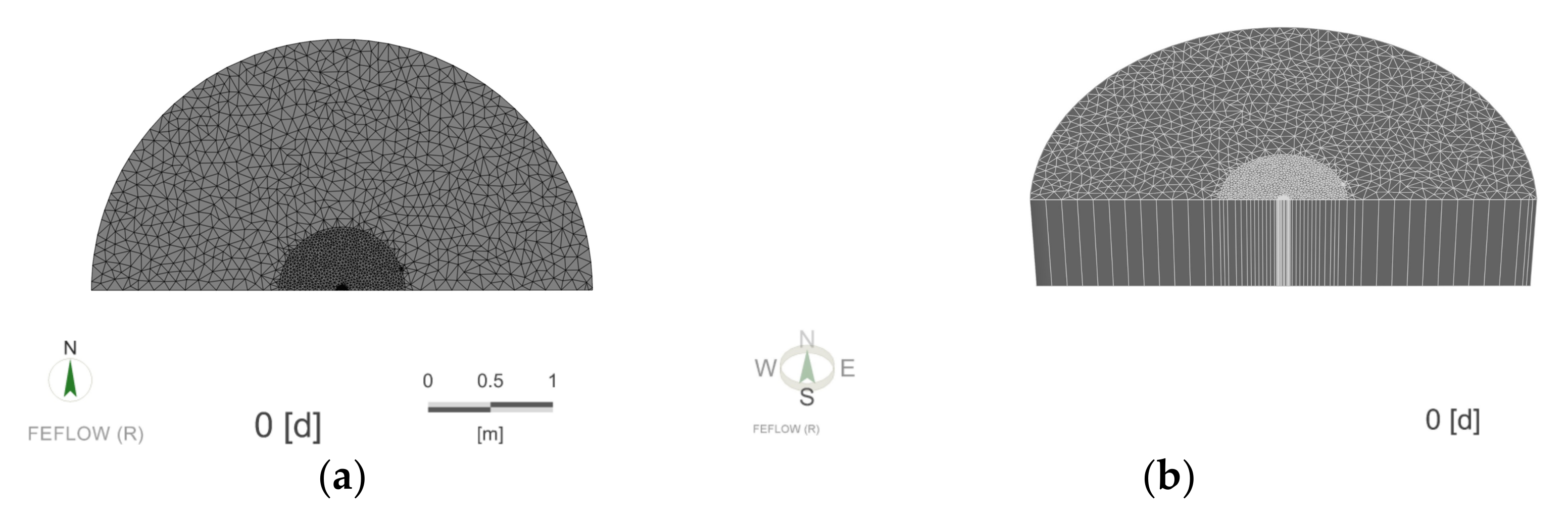
5.1. Numerical Model Establishment of the Slug Heat Test

The FEFLOW finite element 3D model was used to create a numerical model according to the same dimensions and parameters as the indoor test platform. The model was set up as a confined aquifer of the same thickness as the indoor platform aquifer, and was divided in plane into the test well S₀ area and the aquifer area. After establishing the model, the initial conditions, boundary conditions, and media properties of the model need to be assigned according to the parameters of the indoor platform, and the simulation problem type needs to be set. The initial conditions of this simulation are set to the excitation heat source with the same temperature as the indoor model test, and the problem is set to the heat transfer problem in the saturated medium. The arc side boundary of the test platform is equipped with an overflow outlet to keep the constant water head, so the arc side of the numerical model is set as the first type of constant water head and temperature boundary. The glass side of the semi-cylindrical section of the test platform is treated with water and heat insulation, so this boundary in the numerical model is set as the second type of zero flow and zero heat flux boundary. The top and bottom of the confined aquifer are set as the second type of zero-flow and zero-heat flux boundaries, respectively. Observation points were arranged in the test well to observe the temperature change of test section in the test well with time. Mesh generation and local encryption were performed on the simulation model and a 3D model was built, and the built numerical model is shown in Figure 11.

5.2. Analysis of Numerical Simulation

The purpose of the numerical simulation analysis is to assign parameters values according to the thermal properties parameters of the aquifer and rock-soil skeleton obtained from the theoretical model of the slug heat test in the indoor model to the numerical model, to obtain the calculated temperature variation curve of the test well S₀ with time by changing different test conditions of the numerical model and to compare the results with the measured temperature variation curve of the test well with time under the same test conditions to verify the accuracy and reliability of the theoretical model and test method for determining the thermal properties parameters of the aquifers and rock-soil skeletons by the slug heat test.

5.2.1. Analysis of Simulation Results in the Case of u = 0

Three sets of test conditions, $w\left(\Delta T=10 °\mathrm{C}\right)$, $w\left(\Delta T=6 °\mathrm{C}\right)$ and $w\left(\Delta T=4 °\mathrm{C}\right)$, of the indoor test in the case of $u=0$ were used as the basis for setting the parameters of the initial temperature, initial water head, the thermal conductivity of the rock-soil skeleton, heat capacity of the rock-soil skeleton obtained by the theoretical model of the slug heat test and the permeability coefficient of the aquifer of the test model obtained through the pumping test for the numerical model. The specific values are shown in

Table 5. Simulation parameter settings in the case of $u=0$.

Parameters	Simulation Test No.	Value	Unit
Temperature difference $\Delta T$	$\mathrm{mnw}\left(\Delta T=10\right)$	$\Delta T=10$	$°\mathrm{C}$
	$\mathrm{mnw}\left(\Delta T=6\right)$	$\Delta T=6$	$°\mathrm{C}$
	$\mathrm{mnw}\left(\Delta T=4\right)$	$\Delta T=4$	$°\mathrm{C}$
Simulation duration		0.5	d
Aquifer porosity $n$		0.33	/
Thermal conductivity of rock-soil skeleton ${\lambda }_s$		1.51	W/(m·°C)
		1.03
		1.06
Heat capacity of rock-soil skeleton ${\left(\rho c\right)}_s$		$1{.06 \times 10}^6$	${\mathrm{J}/(\mathrm{m}}^3·\mathrm{K})$
Permeability coefficient $k$		0.124	cm/s

.

The model is assigned according to the parameters in Table 5. The numerical model was run and the temperature change of the test section in the test well was observed. The temperature change data obtained from the simulation were compared with the measured temperature change data of the indoor model test. The data during the time of 0 to 1000 s with a large temperature change range were selected to observe the curve shape, as shown in Figure 12.

It can be seen from Figure 12 that the temperature change range for different excitation strengths ($\Delta T=10 °\mathrm{C}$, $\Delta T=6 °\mathrm{C},\Delta T=4 °\mathrm{C}$) in the case of $u=0$ is concentrated in the 0 to 1000 s time period, and the longer recovery time to the initial temperature is required as the higher excitation temperature. The temperature variation curves calculated in the numerical simulation and measured in the indoor model tests have similar shapes. The calculated and measured values have the same law and can be matched well, except that the calculated curve is smoother and the measured curve fluctuates relatively more; however, the variation laws and trends are completely consistent, and the error is mainly due to the accidental error in the process of test operation and data acquisition in the indoor test. This shows that the theoretical model of the slug heat test in the case of $u=0$ can accurately obtain the stagnant thermal conductivity of the aquifer and derive the thermal property parameters of the rock-soil skeleton, which verifies the accuracy and reliability of the theoretical model, calculation method and test method of the slug heat test.

5.2.2. Analysis of the Simulation Results in the Case of u ≠ 0

In the case of u ≠ 0 for the numerical simulation of the slug heat test, the water head difference for three cases ($\Delta h=12 \mathrm{cm}$, $\Delta h=9 \mathrm{cm}$, $\Delta h=6 \mathrm{cm}$) between the test well and the water head of aquifer was selected, and then, three different temperature differences ($\Delta T=7 °\mathrm{C}$, $\Delta T=4 °\mathrm{C}$, $\Delta T=2 °\mathrm{C}$) were, respectively, simulated under these three water head difference conditions. The specific parameter settings are shown in

Table 6. Simulation parameter settings in the case of $u\ne 0$.

Parameters	Simulation Test No.	Value	Unit
Initial conditions	$\mathrm{mny}\left(\Delta h=6~12,\Delta T=2\right)$	$\Delta T=2$	$\mathrm{cm}, °\mathrm{C}$
	$\mathrm{mny}\left(\Delta h=6~12,\Delta T=4\right)$	$\Delta T=4$	$\mathrm{cm}, °\mathrm{C}$
	$\mathrm{mny}\left(\Delta h=6~12,\Delta T=7\right)$	$\Delta T=7$	$\mathrm{cm}, °\mathrm{C}$
Simulation duration		0.5	d
Aquifer porosity $n$		0.33	/
Thermal conductivity of rock-soil skeleton ${\lambda }_s$		1.06	W/(m·°C)
		1.03
		1.51
Heat capacity of rock-soil skeleton ${\left(\rho c\right)}_s$		$1{.06 \times 10}^6$	${\mathrm{J}/(\mathrm{m}}^3·\mathrm{K})$
Permeability coefficient $k$		0.124	cm/s

.

According to Table 6, the parameters of the numerical model in the case of $u\ne 0$ were assigned. The numerical model was run and the temperature change of the test section in the test well was observed. The temperature change data obtained from the simulation were compared with the measured temperature change data of the indoor model test. The data during the time of 0 to 50 s with a large temperature change range were selected to observe the curve shape, as shown in Figure 13.

It can be seen from Figure 13 that temperature variation curves of the numerical model have similar shapes under different seepage conditions and different excitation strengths in the case of $u\ne 0$. Meanwhile, the temperature variation curves obtained from numerical simulations have basically similar shapes with those obtained from indoor model tests, and the calculated and measured values have the same change law. Similarly, only the calculated curve is steadier and smoother, and the measured curve is relatively more fluctuating. The temperature dissipation in the aquifer is faster due to the higher flow rate $u$, which reflects the increase of the effective thermal conductivity. The time for temperature dissipation is longer as the excitation strength is higher. At the same time, it can be seen from Figure 13 that the fitting result of the calculated and measured values is better as there is a smaller water head difference. Meanwhile, in the early stage of the test, the calculated and measured values also fit well, where when the time increases, the decrease of the rate of the calculated value is slower than the decrease of the rate of the measured value. The specific reason for this is that the indoor model test with different flow conditions was conducted by continuously injecting cold water into the test well to maintain a constant water head difference between the test well and the boundary, during which cold water continuously mixes with the heat source and accelerates the temperature dissipation in the test well over time. However, the temperature variation curves obtained from the numerical simulation and measured by the indoor model test have the same laws and trends. Thus, this indicates that the theoretical model of the slug heat test in the case of $u\ne 0$ can accurately obtain the effective thermal conductivity of the aquifer and derive the thermal property parameters of the rock-soil skeleton, which also verifies the accuracy and reliability of the theoretical model, calculation method and test method of the slug heat test.

6. Conclusions

A novel slug heat test method is proposed to determine the thermal property parameters of aquifers and rock-soil skeletons. Based on the theoretical model of the slug heat test under different hydrodynamic conditions, the thermal property parameters of aquifers and rock-soil skeletons are obtained through the indoor model test, and the heat transfer law in the aquifer is investigated. The three research methods of theoretical research, indoor test research and numerical simulation are mutually demonstrated, and the specific conclusions are as follows:

• Based on the thermal radial convection-dispersion theory and the principle of heat conservation, a theoretical model of the slug heat test was established. The theoretical model of the slug heat test was solved by using the Stehfest algorithm and Talbot algorithm to obtain multiple sets of standard curves under different hydrodynamic conditions, and a specific calculation method for determining the thermal property parameters of aquifers and rock-soil skeletons based on the slug heat test was proposed.
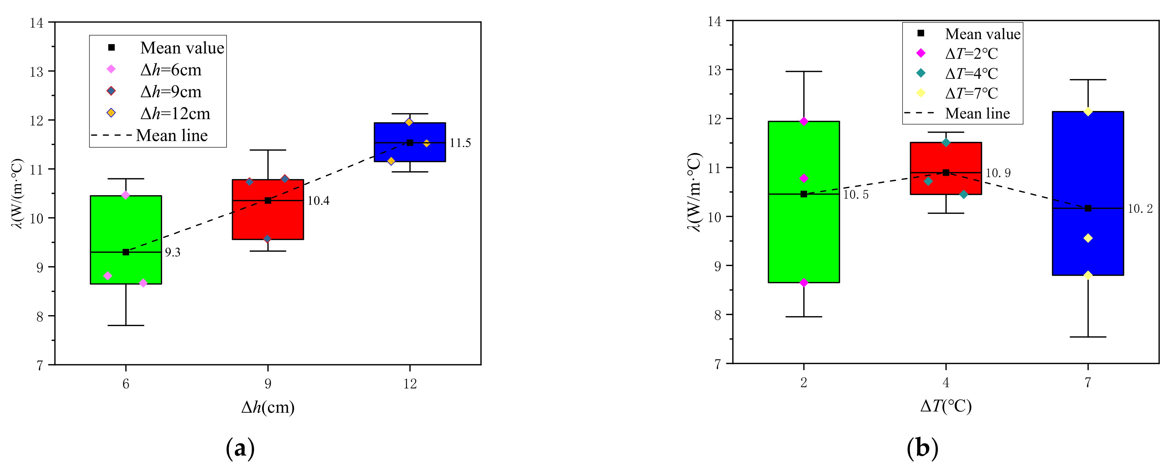
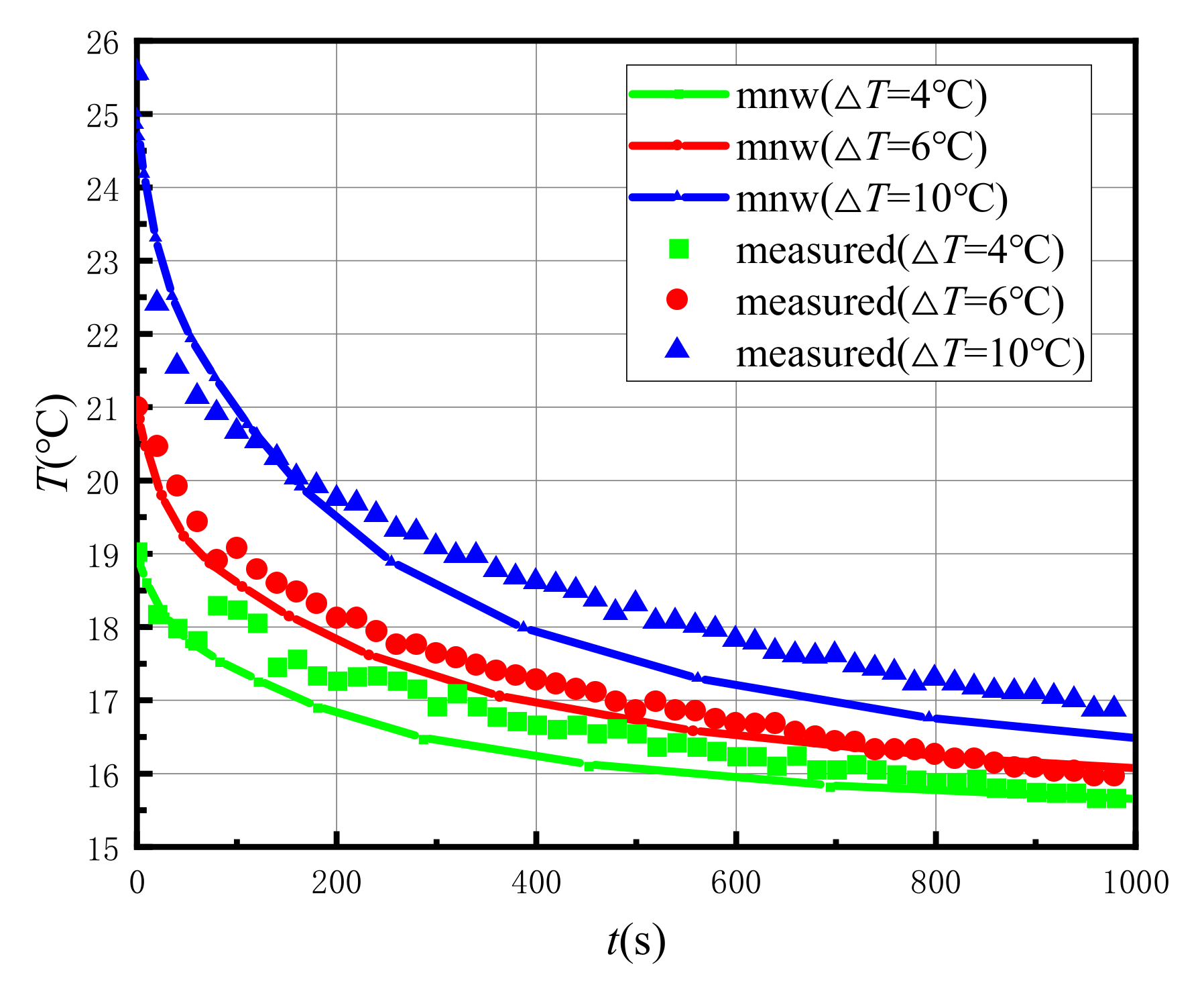
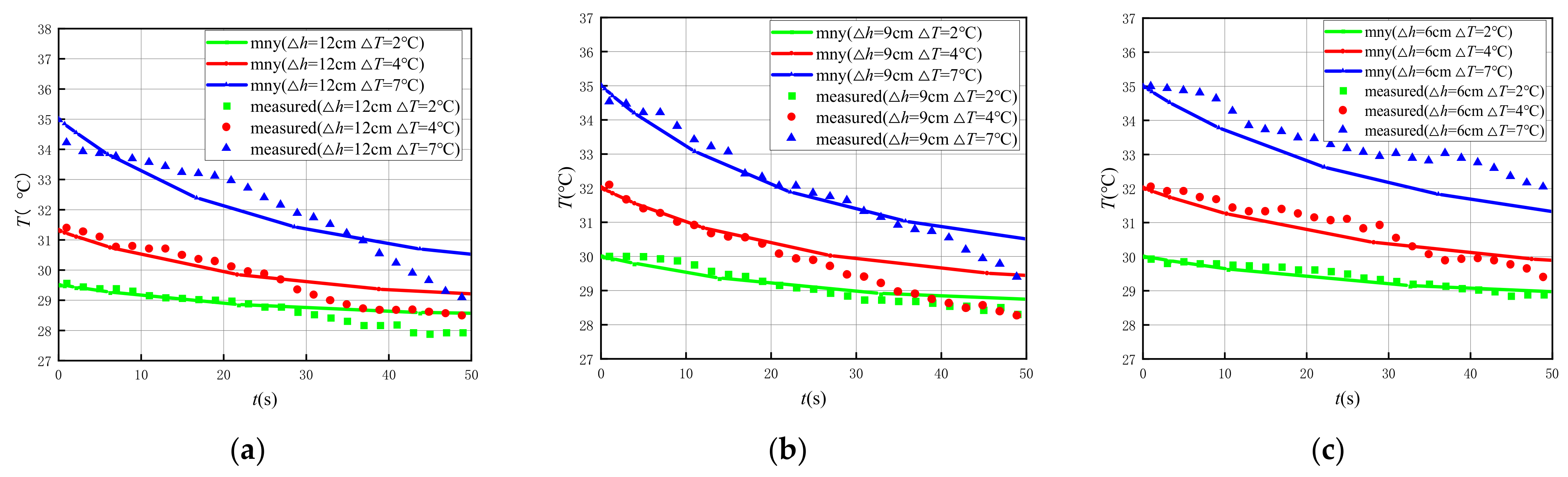
• Slug heat tests were conducted in the indoor confined aquifer platform, and the slug heat test data under different hydrodynamic conditions were fitted with standard curves to obtain the thermal property parameters including effective thermal conductivity, stagnant thermal conductivity, thermal mechanical dispersion coefficient, thermal dispersive degree, thermal diffusivity, heat capacity of aquifer, rock-soil skeletons heat capacity and thermal conductivity. The effective thermal conductivity of the aquifer also clearly increases with the increase of flow rate. The excitation temperature difference had little effect on the effective thermal conductivity of the aquifer. At the same time, the numerical simulation method was used to compare and verify the temperature change laws and trends of simulation calculation values under the same test conditions with measured values with time. The research results show that the slug heat test has the characteristics of high applicability, simple operation and rapid test, and can effectively determine the thermal property parameters of aquifers and rock-soil skeletons.
• The slug heat test model assumes that the radius of the excitation device is the same as the radius of the test well. Therefore, the radius of the excitation device should be as close as possible to the radius of the test well when conducting the slug heat test. In addition, the influences and factors of different seepage conditions and temperature excitation strengths on the calculation results of thermal property parameters of aquifers and rock-soil skeletons by slug heat tests need to be further studied. Meanwhile, since the slug heat test only changes the temperature field in a small range around the test well, the thermal property parameters calculated by the slug heat test only represent the thermal property parameters of the aquifer and the rock-soil skeleton in a small range around the test well, and the scale effect of the slug heat test needs to be further investigated.
• At present, according to the theoretical and indoor test model research conclusions of the slug heat test, the application of slug heat test in fractured rock mass aquifer is uncertain and needs to be further studied. At the same time, since the regular circular hydrogeological boundary is used in the indoor test model, the influence of the irregular hydrogeological boundary of the test site on the slug heat test needs to be further studied in the field test.

References

1. Aresti, L.; Christodoulides, P.; Florides, G. A review of the design aspects of ground heat exchangers. Renew. Sustain. Energy Rev. 2018, 92, 757–773. [Google Scholar] [CrossRef]
2. Zhou, Y.; Zhang, H.; Gui, Z.; Wang, K.; Zhang, Y. Study on influencing factors of comprehensive thermal conductivity of rock and soil. Geol. Surv. China 2018, 5, 89–94. [Google Scholar] [CrossRef]
3. Pan, M.; Huang, Q.; Feng, R.; Huang, G. Estimation of water and heat transfer parameters of saturated silica sand by using different types of data. Trans. Chin. Soc. Agric. Eng. 2020, 36, 75–82. [Google Scholar] [CrossRef]
4. Mo, X.; Di, W.; Liangwen, J.; Jihong, Q. Review on Thermal Conductivity Coefficient of Rock and Soil Mass. J. Earth Sci. Environ. 2011, 33, 421–427+433. [Google Scholar] [CrossRef]
5. Li, B.; Han, Z.; Hu, H.; Bai, C. Study on the effect of groundwater flow on the identification of thermal properties of soils. Renew. Energy 2020, 147, 2688–2695. [Google Scholar] [CrossRef]
6. Yuqun, X.; X. C. Study on Heat Transfer in Porous Media. Geotech. Investig. Surv. 1990, 3, 27–32. [Google Scholar]
7. Van der Heijde, P.; Bachmat, Y.; Bredehoeft, J.; Andrews, B.; Holtz, D.; Sebastian, S. Groundwater Management: The Use of Numerical Models; American Geophysical Union: Washington, DC, USA, 1980; Volume 5. [Google Scholar]
8. Wu, Z.-W.; Song, H.-Z. Numerical simulation of thermal convection in shallow ground temperature field. Yantu Lixue Rock Soil Mech. 2010, 31, 1303–1308. [Google Scholar]
9. Liu, G.-Q.; Zhou, Z.-F.; Li, Z.-F.; Zhou, Y.-Z. Experimental study of heat transfer and thermal dispersion effect assessment in small scale aquifer. Yantu Lixue Rock Soil Mech. 2015, 36, 171–177. [Google Scholar] [CrossRef]
10. Zhang, L.; Zhao, L.; Yang, L.; Songtao, H. Analyses on soil temperature responses to intermittent heat rejection from BHEs in soils with groundwater advection. Energy Build. 2015, 107, 355–365. [Google Scholar] [CrossRef]
11. Spitler, J.D.; Javed, S.; Ramstad, R.K. Natural convection in groundwater-filled boreholes used as ground heat exchangers. Appl. Energy 2016, 164, 352–365. [Google Scholar] [CrossRef]
12. Wei, L.F.A.; Xiaoming, H. Theory and Application of Heat and Mass Transfer in Porous Media; Science Press: Beijing, China, 2006. [Google Scholar]
13. Predvoditelev, A.; Pomerantsev, A.; Bubnov, V. Heat and Mass Transfer (Handbook): A. V. Luikov, Energiya, Moscow (1972). Int. J. Heat Mass Transf. 1973, 16, 1062–1063. [Google Scholar] [CrossRef]
14. Palmer, C.D.; Blowes, D.W.; Frind, E.O.; Molson, J.W. Thermal energy storage in an unconfined aquifer: 1. Field Injection Experiment. Water Resour. Res. 1992, 28, 2845–2856. [Google Scholar] [CrossRef]
15. Molina-Giraldo, N.; Bayer, P.; Blum, P. Evaluating the influence of thermal dispersion on temperature plumes from geothermal systems using analytical solutions. Int. J. Therm. Sci. 2011, 50, 1223–1231. [Google Scholar] [CrossRef]
16. Metzger, T.; Didierjean, S.; Maillet, D. Optimal experimental estimation of thermal dispersion coefficients in porous media. Int. J. Heat Mass Transf. 2004, 47, 3341–3353. [Google Scholar] [CrossRef]
17. Xue, Y.; Xie, C.; Li, Q. A Thermal Energy Storage Model for a Confined Aquifer. Dev. Water Sci. 1988, 36, 337–342. [Google Scholar] [CrossRef]
18. Hailin, Z. Theoretical and Experimental Research on the Model Accuracy Improvement of Effective Thermal Conductivity of the Disperse System; North China Electric Power University: Hebei, China, 2004. [Google Scholar]
19. Shi, Y.-F.; Liu, H.; Sun, W.-C. Experiment and numerical simulation of effective thermal conductivity of porous media. Sichuan Daxue Xuebao Gongcheng Kexue Ban J. Sichuan Univ. 2011, 43, 198–203. [Google Scholar] [CrossRef]
20. Albert, K.; Franz, C.; Koenigsdorff, R.; Zosseder, K. Inverse estimation of rock thermal conductivity based on numerical microscale modeling from sandstone thin sections. Eng. Geol. 2017, 231, 1–8. [Google Scholar] [CrossRef]
21. Alishaev, M.; Abdulagatov, I.; Abdulagatova, Z. Effective thermal conductivity of fluid-saturated rocks: Experiment and modeling. Eng. Geol. 2012, 135–136, 24–39. [Google Scholar] [CrossRef]
22. Zhang, Y.; Hao, S.; Yu, Z.; Fang, J.; Zhang, J.; Yu, X. Comparison of test methods for shallow layered rock thermal conductivity between in situ distributed thermal response tests and laboratory test based on drilling in northeast China. Energy Build. 2018, 173, 634–648. [Google Scholar] [CrossRef]
23. Yu, M.Z.; Peng, X.F.; Li, X.D.; Fang, Z.H. A Simplified Model for Measuring Thermal Properties of Deep Ground Soil. Exp. Heat Transf. 2004, 17, 119–130. [Google Scholar] [CrossRef]
24. Mogensen, P. Fluid to duct wall heat transfer in duct system heat storages. In Proceedings of the International Conference on Subsurface Heat Storage in Theory and Practice, Stockholm, Sweden, 6–8 June 1983; Volume 16, pp. 652–657. [Google Scholar]
25. Wang, S.; You, S.; Zhang, G. Application of geo-thermal response test in the design of ground heat exchanger. Taiyangneng Xuebao Acta Energ. Sol. Sin. 2007, 28, 405–409. [Google Scholar] [CrossRef]
26. Kwong, S.S.; Smith, J.M. Radial Heat Transfer in Packed Beds. Ind. Eng. Chem. 2002, 49, 894–903. [Google Scholar] [CrossRef]
27. Côté, J.; Konrad, J.-M. Assessment of structure effects on the thermal conductivity of two-phase porous geomaterials. Int. J. Heat Mass Transf. 2009, 52, 796–804. [Google Scholar] [CrossRef]
28. Carson, J.K.; Sekhon, J.P. Simple determination of the thermal conductivity of the solid phase of particulate materials. Int. Commun. Heat Mass Transf. 2010, 37, 1226–1229. [Google Scholar] [CrossRef]
29. Xiaolin, Z. The Research of Effective Conductivity in the Porous Media; Dalian University of Technology: Dalian, China, 2009. [Google Scholar]
30. Shi, M.-H.F.H. A Fractal Modal for Evaluating Heat Conduction in Porous Media. J. Therm. Sci. Technol. 2002, 28–31. [Google Scholar] [CrossRef]
31. Yu, B.; Li, J. Some Fractal Characters of Porous Media. Fractals Complex Geom. Patterns Scaling Nat. Soc. 2001, 9, 365–372. [Google Scholar] [CrossRef]
32. Qin, X.; Cai, J.; Xu, P.; Dai, S.; Gan, Q. A fractal model of effective thermal conductivity for porous media with various liquid saturation. Int. J. Heat Mass Transf. 2019, 128, 1149–1156. [Google Scholar] [CrossRef]
33. Shen, Y.; Xu, P.; Qiu, S.; Rao, B.; Yu, B. A generalized thermal conductivity model for unsaturated porous media with fractal geometry. Int. J. Heat Mass Transf. 2020, 152, 119540. [Google Scholar] [CrossRef]
34. Feng, Y.; Yu, B.; Zou, M.; Xu, P. A Generalized Model for the Effective Thermal Conductivity of Unsaturated Porous Media Based on Self-Similarity. J. Porous Media 2007, 10, 551–568. [Google Scholar] [CrossRef]
35. Yanrong, Z.; Zhifang, Z. Comparative study on field slug tests to determine aquifer permeability based on Kipp model and CBP model. Geotech. Investig. Surv. 2012, 40, 32–38. [Google Scholar]
36. McElwee, C. Improving the analysis of slug tests. J. Hydrol. 2002, 269, 122–133. [Google Scholar] [CrossRef]
37. Zhao, Y.-R.; Zhou, Z.-F. A Field Test Data Research Based on a New Hydraulic Parameters Quick Test Technology. J. Hydrodyn. 2010, 22, 562–571. [Google Scholar] [CrossRef]
38. Zhao, Y.; Wei, Y.; Dong, X.; Rong, R.; Wang, J.; Wang, H. The Application and Analysis of Slug Test on Determining the Permeability Parameters of Fractured Rock Mass. Appl. Sci. 2022, 12, 7569. [Google Scholar] [CrossRef]
39. Zhao, Y.; Zhang, Z.; Rong, R.; Dong, X.; Wang, J. A new calculation method for hydrogeological parameters from unsteady-flow pumping tests with a circular constant water-head boundary of finite scale. Q. J. Eng. Geol. Hydrogeol. 2022, 55. [Google Scholar] [CrossRef]
40. Zhifang, Z. Groudwater Dynamics; Science Press: Beijing, China, 2013. [Google Scholar]
41. Caisheng, C. Equations of Mathematical Physics; Science Press: Beijing, China, 2008. [Google Scholar]
42. Fu, Z.-J.; Chen, W.; Qin, Q.-H. Three Boundary Meshless Methods for Heat Conduction Analysis in Nonlinear FGMs with Kirchhoff and Laplace Transformation. Adv. Appl. Math. Mech. 2012, 4, 519–542. [Google Scholar] [CrossRef]
43. D’Amore, L.; Mele, V.; Campagna, R. Quality assurance of Gaver’s formula for multi-precision Laplace transform inversion in real case. Inverse Probl. Sci. Eng. 2017, 26, 553–580. [Google Scholar] [CrossRef]
44. Tsai, X.Q.F.Z.C.-C. Heat conduction solution of nonlinear functionally graded material based on fundamental solution method combined with extended precision arithmetic. Comput. Aided Eng. 2016, 25, 7–14+22. [Google Scholar] [CrossRef]
45. Yuqun, X.X.C. Numerical Simulation for Groundwater; Science Press: Beijing, China, 2007. [Google Scholar]
Figure 1. Schematic diagram of the slug heat test model (The blue dashed line represents the outer wall of the screen pipe, and the red dashed line represents the outer wall of heat excitation device. Red area represents the internal structure of the heat excitation device).
Water 14 03020 g001
Figure 2. T * D ~ τ semi-logarithmic standard curves for different α and γ parameters in the case of u = 0 .
Water 14 03020 g002
Figure 3. T * D ~ τ double logarithmic standard curves for different α , γ , β parameters in the case of u 0 . (a) β = 0 ; (b) β = 0.5 ; (c) β = 1 .
Water 14 03020 g003
Figure 4. Indoor test platform. (a) Front view of the test platform (The red arrow indicates thermal convection-dispersion direction); (b) Top view of the test platform ( # indicates the number of temperature sensor).
Water 14 03020 g004
Figure 5. Physical picture of the test platform. (a) Appearance of the test platform frame; (b) Internal construction of aquifer system.
Water 14 03020 g005
Figure 6. Temperature variation curve of the test well with different excitation strengths during slug heat tests in the case of u = 0 .
Water 14 03020 g006
Figure 7. Matching diagram for different excitation strengths in the test well in the case of u = 0 . (a) w Δ T = 4   ° C 1 ; (b) w Δ T = 4   ° C 2 ; (c) w Δ T = 6   ° C 1 ; (d) w Δ T = 6   ° C 2 ; (e) w Δ T = 10   ° C 1 ; (f) w Δ T = 10   ° C 2 .
Water 14 03020 g007
Figure 8. Temperature variation curve of the test well with different excitation strengths during slug heat tests in the case of u 0 . (a) Δ h = 6   cm ; (b) Δ h = 9   cm ; (c) Δ h = 12   cm .
Water 14 03020 g008
Figure 9. Matching diagram for different test conditions in the test well in the case of u 0 . (a) y Δ h = 6   cm   Δ T = 2   ° C 1 ; (b) y Δ h = 6   cm   Δ T = 2   ° C 2 ; (c) y Δ h = 9   cm   Δ T = 2   ° C 1 ; (d) y Δ h = 9   cm   Δ T = 2   ° C 2 ; (e) y Δ h = 12   cm   Δ T = 2   ° C 1 ; (f) y Δ h = 12   cm   Δ T = 2   ° C 2 ; (g) y Δ h = 6   cm   Δ T = 4   ° C 1 ; (h) y Δ h = 6   cm   Δ T = 4   ° C 2 ; (i) y Δ h = 9   cm   Δ T = 4   ° C 1 ; (j) y Δ h = 9   cm   Δ T = 4   ° C 2 ; (k) y Δ h = 12   cm   Δ T = 4   ° C 1 ; (l) y Δ h = 12   cm   Δ T = 4   ° C 2 ; (m) y Δ h = 6   cm   Δ T = 7   ° C 1 ; (n) y Δ h = 6   cm   Δ T = 7   ° C 2 ; (o) y Δ h = 9   cm   Δ T = 7   ° C 1 ; (p) y Δ h = 9   cm   Δ T = 7   ° C 2 ; (q) y Δ h = 12   cm   Δ T = 7   ° C 1 ; (r) y Δ h = 12   cm   Δ T = 7   ° C 2 .
Water 14 03020 g009aWater 14 03020 g009b
Figure 10. Calculated value of effective thermal conductivity in the case of u 0 . (a) Calculated values of effective thermal conductivity for different flow rates (The colors of green, red, blue respectively correspond to data sets under three different water head differences); (b) Calculated values of effective thermal conductivity for different excitation strengths (The colors of green, red, blue respectively correspond to the data sets under three different heat excitation strengths).
Water 14 03020 g010
Figure 11. Numerical model diagram. (a) Mesh generation; (b) 3D model building.
Water 14 03020 g011
Figure 12. Comparison of the temperature variation of the test section in the test well under different excitation strengths between the numerical simulation and the measured value in the case of u = 0 .
Water 14 03020 g012
Figure 13. Comparison of temperature variation of test section in the test well under different excitation strengths between numerical simulation and the measured value in the case of u 0 . (a) Δ h = 12 ; (b) Δ h = 9 ; (c) Δ h = 6 .
Water 14 03020 g013